2 Governing equations and dispersion relation

Consider the propagation of internal waves in an inviscid, incompressible, adiabatic and stably stratified fluid of density $\unicode[STIX]{x1D70C}(x,y,z,t)$ , bounded by a free surface on the top and a rigid sea floor at the depth $h$ . Let’s define a Cartesian coordinate system with $x,y$ -axes on the mean free surface and $z$ -axis positive upward. Newton’s second law, conservation of mass and conservation of salt provide five equations for the evolution of the components of the velocity vector $\boldsymbol{u}=\{u,v,w\}$ , density $\unicode[STIX]{x1D70C}$ and the pressure $p$ . These governing equations under Boussinesq approximation together with three boundary conditions (two kinematic boundary conditions on the free surface and the seabed, and one dynamic boundary condition on the free surface) uniquely determine the five unknowns and the surface elevation $\unicode[STIX]{x1D702}(x,y,t)$ (e.g. Thorpe Reference Thorpe1966).

We assume internal waves are small perturbations to a stable background state at equilibrium. Therefore, density can be written as $\unicode[STIX]{x1D70C}(x,y,z,t)=\bar{\unicode[STIX]{x1D70C}}(z)+\unicode[STIX]{x1D70C}^{\prime }(x,y,z,t)$ where $\bar{\unicode[STIX]{x1D70C}}(z)$ is the background (unperturbed) density. Similarly, we define a pressure perturbation $p^{\prime }$ via $p=\bar{p}(z)+p^{\prime }(x,y,z,t)$ such that $\text{d}\bar{p}(z)/\text{d}z=-\bar{\unicode[STIX]{x1D70C}}(z)g$ . With some standard manipulation, the governing equations can be written in terms of any of the five variables involved in this problem. We choose to write the equation, as is customary, in terms of the vertical component of the velocity, $w$ . These equations then read (see e.g. Thorpe Reference Thorpe1966, or appendix A)

(2.1a ) $$\begin{eqnarray}\displaystyle & \displaystyle \frac{\unicode[STIX]{x2202}^{2}}{\unicode[STIX]{x2202}t^{2}}\unicode[STIX]{x1D6FB}^{2}w+N^{2}\unicode[STIX]{x1D6FB}_{H}^{2}w={\mathcal{E}}(\boldsymbol{u},\unicode[STIX]{x1D70C}^{\prime }),\quad -h<z<\unicode[STIX]{x1D702}, & \displaystyle\end{eqnarray}$$

(2.1b ) $$\begin{eqnarray}\displaystyle & \displaystyle \frac{\unicode[STIX]{x2202}^{3}w}{\unicode[STIX]{x2202}z\unicode[STIX]{x2202}t^{2}}-g\unicode[STIX]{x1D6FB}_{H}^{2}w={\mathcal{F}}(\boldsymbol{u},p^{\prime },\unicode[STIX]{x1D702}),\quad z=0, & \displaystyle\end{eqnarray}$$

(2.1c ) $$\begin{eqnarray}\displaystyle & \displaystyle w=0,\quad z=-h, & \displaystyle\end{eqnarray}$$

$\unicode[STIX]{x1D6FB}_{H}^{2}=\unicode[STIX]{x2202}^{2}/\unicode[STIX]{x2202}x^{2}+\unicode[STIX]{x2202}^{2}/\unicode[STIX]{x2202}y^{2}$

$N^{2}=-(g/\unicode[STIX]{x1D70C}_{0})\,\text{d}\bar{\unicode[STIX]{x1D70C}}(z)/\text{d}z$

$\unicode[STIX]{x1D70C}_{0}=\bar{\unicode[STIX]{x1D70C}}(z=0)$

${\mathcal{E}},{\mathcal{F}}$

To perform a perturbation analysis, we assume that the solution to (2.1) can be expressed in terms of a convergent series, i.e.

(2.2) $$\begin{eqnarray}\displaystyle w(\boldsymbol{x},t)=\unicode[STIX]{x1D716}w^{(1)}(\boldsymbol{x},t)+\unicode[STIX]{x1D716}^{2}w^{(2)}(\boldsymbol{x},t)+O(\unicode[STIX]{x1D716}^{3}), & & \displaystyle\end{eqnarray}$$

where $\unicode[STIX]{x1D716}\ll 1$ is a measure of steepness of the waves involved and $w^{(i)}\sim O(1)$ . Similar expressions hold for $u,v,\unicode[STIX]{x1D70C}^{\prime }$ and $p^{\prime }$ . Substituting (2.2) into (2.1) and collecting terms of the same magnitude, then at the leading order $O(\unicode[STIX]{x1D716})$ the linearized equations are obtained.

Figure 1.

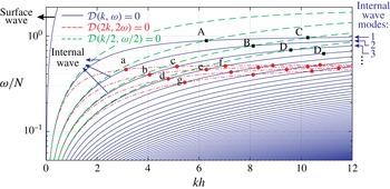
Plot of the dimensionless frequency $\unicode[STIX]{x1D714}/N$ as a function of dimensionless wavenumber $kh$ of free internal waves (i.e.  ${\mathcal{D}}(k,\unicode[STIX]{x1D714})=0$ ) in a fluid of linearly stratified density $\unicode[STIX]{x1D70C}(z)=\unicode[STIX]{x1D70C}_{0}(1-az)$ , with $ah=0.05$ . Associated with each wavenumber there is one surface wave and an infinite number of internal wave modes (blue solid-line branches). The frequency of internal waves cannot exceed the Brunt–Väisälä frequency $N$ , and all branches of the dispersion relation curve are capped at $\unicode[STIX]{x1D714}/N=1$ . We also plot contours of ${\mathcal{D}}(2k,2\unicode[STIX]{x1D714})=0$ (red dash-dotted lines) whose intersections with blue lines (shown by red circles) mark waves whose second harmonics are also solutions to the dispersion relation. These second harmonics are at the intersections of contours of ${\mathcal{D}}(k/2,\unicode[STIX]{x1D714}/2)=0$ (green dashed lines) and ${\mathcal{D}}(k,\unicode[STIX]{x1D714})=0$ and are marked by black squares. The second harmonic of the wave at ‘a’ (mode 2), is the wave ‘A’ (mode 1) and so on.

We focus our attention here on the two-dimensional problem with a linear mean density profile, i.e.  $\bar{\unicode[STIX]{x1D70C}}(z)=\unicode[STIX]{x1D70C}_{0}(1-az)$ which gives a constant Brunt–Väisälä frequency $N=\sqrt{ga}$ (cf. e.g. Martin, Simmons & Wunsch Reference Martin, Simmons and Wunsch1972). Looking for a progressive wave solution of the leading-order (linearized) equation in the form $w^{(1)}=W(z)\sin (\boldsymbol{k}\boldsymbol{\cdot }\boldsymbol{x}-\unicode[STIX]{x1D714}t)$ the following dispersion relations result:

(2.3) $$\begin{eqnarray}\displaystyle {\mathcal{D}}(k,\unicode[STIX]{x1D714})=\left\{\begin{array}{@{}ll@{}}\displaystyle \unicode[STIX]{x1D714}^{2}-\frac{gk}{\sqrt{1-N^{2}/\unicode[STIX]{x1D714}^{2}}}\tanh \left(kh\sqrt{1-N^{2}/\unicode[STIX]{x1D714}^{2}}\right)=0,\quad & \unicode[STIX]{x1D714}>N\\ \displaystyle \unicode[STIX]{x1D714}^{2}-\frac{gk}{\sqrt{N^{2}/\unicode[STIX]{x1D714}^{2}-1}}\tan \left(kh\sqrt{N^{2}/\unicode[STIX]{x1D714}^{2}-1}\right)=0,\quad & \unicode[STIX]{x1D714}<N.\end{array}\right. & & \displaystyle\end{eqnarray}$$

Solutions to the above dispersion relation identify permissible frequencies and wavenumbers of free propagating waves. Contours of ${\mathcal{D}}(k,\unicode[STIX]{x1D714})=0$ are shown in figure 1 in which we plot the dimensionless frequency $\unicode[STIX]{x1D714}/N$ as a function of dimensionless wavenumber $kh$ (blue solid curves). For $\unicode[STIX]{x1D714}>N$ only one solution exists in the first quadrant (with its mirror in the other quadrants). This solution corresponds to a wave whose associated fluid particle motion is maximum near the free surface and decreases as the depth increases. Therefore this is basically a classical surface wave which is perturbed slightly because of stratification. For $\unicode[STIX]{x1D714}<N$ there is an infinite number of solutions to (2.3). The first member of this set, is the continuation of the surface wave branch (the leftmost branch in figure 1), but the rest identify waves with associated fluid particles’ vertical velocities $w$ that are zero at the seabed and close to zero near the free surface, but gain one (or more) maximum/maxima somewhere inside the fluid domain. Therefore these branches show internal waves. The number of maxima in the amplitude of the vertical velocity $w$ along the vertical water line determines the mode number of the branch (the first three are marked on the right-hand side of figure 1 with arrows). A cutoff frequency $\unicode[STIX]{x1D714}/N=1$ sets an upper frequency limit for internal waves. We would like to emphasize that the free surface boundary condition, in comparison with the rigid-lid case, leads to a drastically different expressions for mode structures and the dispersion relation. Nevertheless, the curves of the dispersion relation (2.2) are very close to the one under the rigid-lid assumption $\unicode[STIX]{x1D714}=N/\sqrt{1+(n\unicode[STIX]{x03C0}/kh)^{2}}$ .

It can be seen from figure 1 that second-harmonic waves are at least one mode lower than the original waves. Therefore, clearly a mode-1 internal wave can never generate a second harmonic, since its second harmonic must be a mode zero which is non-existent. But mode-2 internal waves can go unstable and resonate mode-1 waves. Therefore, in an internal wave spectrum, there might be mode-1 waves whose origin is different from the origin of the rest of the incident mode-1 internal waves; that is, they are results of instability of mode-2 (and other higher modes) internal waves.

We would like to comment that the dominant energy in the baroclinic tide, which is the most relevant case for the ocean, is in the mode-1 waves. However, most of the prevalent low-mode internal waves (including mode 1) are eventually dissipated through their energy being transferred to waves with higher vertical wavenumbers (see e.g. Garrett Reference Garrett2003). This happens through a number of mechanisms including, for instance, parametric subharmonic instability (aka PSI, e.g. Davis & Acrivos Reference Davis and Acrivos1967) and interaction with the bottom topography (e.g. Bühler & Holmes-Cerfon Reference Bühler and Holmes-Cerfon2011; Couston, Liang & Alam Reference Couston, Liang and Alam2016; Karimpour, Zareei & Alam Reference Karimpour, Zareei and Alam2016). Resonant harmonic generation studied here may interfere, potentially substantially, in this process of energy exchange between different modes. In other words, the mechanism studied here can influence the internal wave spectral evolution by opening up a new avenue for the energy exchange between different modes.

3 Harmonic generation

With the linear solution to (2.1) and its properties at hand, we move to the second-order equation by collecting $O(\unicode[STIX]{x1D716}^{2})$ terms obtained from the substitution of (2.2) into (2.1). The second-order equation has the exact same form as of the leading-order equation on its left-hand side, but with nonlinear terms, arising from the nonlinear functions ${\mathcal{E}},{\mathcal{F}}$ , on its right-hand side. These nonlinear terms are multiplication of the linear solution (and its derivatives) and, it turns out that, they constitute forcing terms with wavenumber and frequency $(2k,2\unicode[STIX]{x1D714})$ . Now if ${\mathcal{D}}(2k,2\unicode[STIX]{x1D714})=0$ , then it means that these forcing terms have a harmonic which is the same as the natural harmonic of the linear system. This is a resonance scenario through which a new second-order solution may emerge and may grow large enough to the extent that it becomes comparable to the leading-order solution. We would like to note a subtle point here that at the second order the right-hand side of (2.1a ) is identically zero (see e.g. Tabaei, Akylas & Lamb Reference Tabaei, Akylas and Lamb2005). Therefore a potential harmonic-generation resonance is only possible through the nonlinear terms in the free surface boundary condition (2.1b ). If a rigid-lid assumption or a linearized form of the free surface boundary condition is employed (which is usually the case in the investigation of internal waves) the resonance harmonic generation will simply not obtain unless a non-uniform stratification or Boussinesq terms are considered.

Figure 2.

There are countably infinite number of internal waves that are unstable to their second harmonic. Physically this means that specific incident internal waves of wavenumber and frequency ( $k,\unicode[STIX]{x1D714}$ ) will give up their energy permanently (in a one-way irreversible process, cf. (4.2)) to their second harmonic ( $2k,2\unicode[STIX]{x1D714}$ ). The necessary condition for this to happen is ${\mathcal{D}}(k,\unicode[STIX]{x1D714})={\mathcal{D}}(2k,2\unicode[STIX]{x1D714})=0$ . 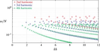These waves, for the parameters of figure 1, are shown here by red squares. Similar story holds for another set of waves that are unstable to their third harmonic (blue circles, necessary condition ${\mathcal{D}}(k,\unicode[STIX]{x1D714})={\mathcal{D}}(3k,3\unicode[STIX]{x1D714})=0$ ) and fourth harmonic (green triangles, ${\mathcal{D}}(k,\unicode[STIX]{x1D714})={\mathcal{D}}(4k,4\unicode[STIX]{x1D714})=0$ ) and so on.

To see whether it is possible to satisfy the resonance condition required for the second harmonic of an internal wave to exist as a free propagating wave, we also plot in figure 1 the contours of ${\mathcal{D}}(2k,2\unicode[STIX]{x1D714})=0$ (red dash-dotted curves) for the first four internal wave modes. Intersections of these contours with the contours of ${\mathcal{D}}(k,\unicode[STIX]{x1D714})=0$ (solid blue curves) identify waves whose second harmonics are also solutions to the dispersion relation. Some of these intersections are marked in figure 1 by red circles and are identified by lowercase characters. It is easy to find the corresponding second harmonic by multiplying a designated (red circle) frequency and wavenumber by a factor of two, or alternatively by finding intersections of contours of ${\mathcal{D}}(k/2,\unicode[STIX]{x1D714}/2)=0$ (green dashed curves) and ${\mathcal{D}}(k,\unicode[STIX]{x1D714})$ (denoted by black squares and uppercase characters). Specifically, ‘A’ is the second harmonic of ‘a’, ‘B’ is the second harmonic of ‘b’ and so on. It is to be noted that the second harmonic of an internal wave always belongs to a lower mode than the mode of the original wave. For example, the second harmonic of wave ‘a’ (mode 2) is the wave ‘A’ (mode 1) and the second harmonic of wave ‘c’ (mode 3) is the wave ‘C’ (mode 1).

A comprehensive collection of all internal waves (for $kh<12$ ) whose second harmonics are also free propagating waves is shown in figure 2. We are basically plotting in this figure all intersections points of contours of ${\mathcal{D}}(k,\unicode[STIX]{x1D714})=0$ and contours of ${\mathcal{D}}(2k,2\unicode[STIX]{x1D714})=0$ . Clearly there will be an infinite (but countable) number of such solutions. Through the approach described above, a similar exercise can be performed for waves with their third harmonic being free waves. These solutions are marked by blue circles in figure 2, and waves with their fourth harmonics lying on the dispersion relation curves are shown by green triangles, and this search can continue indefinitely. In a weakly nonlinear wave propagation problem, instabilities to higher harmonics (e.g. third, fourth, etc.) are much weaker compared with the instability to the second harmonic. This is because the expression for the amplitude growth of higher harmonics contains higher-order perturbation terms. Specifically, if $\unicode[STIX]{x1D716}$ is a measure of a wave steepness, then the amplitude growth rate of its second-harmonic wave is of $O(\unicode[STIX]{x1D716}^{2})$ , but if its third harmonic is excited, then the growth rate is of $O(\unicode[STIX]{x1D716}^{3})$ (cf. the difference between Class I and Class II/III Bragg resonance, e.g. Alam, Liu & Yue Reference Alam, Liu and Yue2009a ).

4 Results and discussion

To determine the strength of the resonance (i.e. the rate of growth of the resonant wave), and the dynamics of the energy interplay between a wave and its second harmonic, here we perform a multiple scale perturbation analysis. The basic assumption is that the original wave and its second harmonic are both functions of spatial variables and time (i.e.  $\boldsymbol{x},t$ ), as well as a slow spatial variable in the direction of propagation $x_{1}=\unicode[STIX]{x1D716}x$ . Physically speaking, we allow the amplitude of both waves to slowly vary as waves propagate. Mathematically speaking this is written as

(4.1) $$\begin{eqnarray}\displaystyle w(x,x_{1},z,t)=\unicode[STIX]{x1D716}w_{1}(x,x_{1},z,t)+\unicode[STIX]{x1D716}^{2}w_{2}(x,x_{1},z,t)+O(\unicode[STIX]{x1D716}^{3}), & & \displaystyle\end{eqnarray}$$

where $w_{i}\sim O(1)$ . Expressions of the same form are assumed to hold for other variables $u,\unicode[STIX]{x1D70C}^{\prime },p^{\prime }$ and $\unicode[STIX]{x1D702}$ . Similar to regular perturbation methodology, described earlier in the paper to gain insight into the problem, we substitute (4.1) into the governing equation (2.1) and collect terms of the same order in $\unicode[STIX]{x1D716}$ . We assume the original wave with wavenumber and frequency $k,\unicode[STIX]{x1D714}$ has the amplitude ${\mathcal{A}}_{1}(x_{1})$ and the amplitude of resonant second-harmonic wave with wavenumber and frequency $2k,2\unicode[STIX]{x1D714}$ is ${\mathcal{B}}_{2}(x_{1})$ . At the second order, applying a compatibility condition (to avoid unbounded solutions) the following two equations governing spatial evolution of ${\mathcal{A}}_{1}(x_{1})$ and ${\mathcal{B}}_{2}(x_{1})$ emerge (see appendix A for details of derivation)

(4.2a ) $$\begin{eqnarray}\displaystyle & \displaystyle \frac{\text{d}{\mathcal{B}}_{2}(x_{1})}{\text{d}x}=\unicode[STIX]{x1D6FC}{\mathcal{A}}_{1}^{2}(x_{1}), & \displaystyle\end{eqnarray}$$

(4.2b ) $$\begin{eqnarray}\displaystyle & \displaystyle \frac{\text{d}{\mathcal{A}}_{1}(x_{1})}{\text{d}x}=\unicode[STIX]{x1D6FD}{\mathcal{A}}_{1}(x_{1}){\mathcal{B}}_{2}(x_{1}), & \displaystyle\end{eqnarray}$$

(4.3) $$\begin{eqnarray}\displaystyle & \displaystyle \unicode[STIX]{x1D6FC}=-\frac{6m_{1}^{2}\unicode[STIX]{x1D714}\cos m_{2}h}{gk(2m_{2}h+\sin 2m_{2}h)}, & \displaystyle\end{eqnarray}$$

(4.4) $$\begin{eqnarray}\displaystyle & \displaystyle \unicode[STIX]{x1D6FD}=-\frac{k[\sin m_{2}h(4m_{1}\cos ^{2}m_{1}h-3m_{1})-2m_{2}\cos m_{2}h\sin 2m_{1}h]}{2\unicode[STIX]{x1D714}(2m_{1}h+\sin 2m_{1}h)}, & \displaystyle\end{eqnarray}$$

in which $m_{1}=k\sqrt{N^{2}-\unicode[STIX]{x1D714}^{2}}/\unicode[STIX]{x1D714}$ and $m_{2}=k\sqrt{N^{2}-4\unicode[STIX]{x1D714}^{2}}/\unicode[STIX]{x1D714}$ .

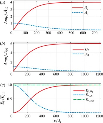
Spatial evolution of the normalized amplitude of the original wave ${\mathcal{A}}_{1}/{\mathcal{A}}_{10}$ (where ${\mathcal{A}}_{10}={\mathcal{A}}_{1}(x=0)$ ) and its second harmonic ${\mathcal{B}}_{2}/{\mathcal{A}}_{10}$ as a function of spatial distance of propagation $x/\unicode[STIX]{x1D706}_{i}$ (where $\unicode[STIX]{x1D706}_{i}=2\unicode[STIX]{x03C0}/k=\text{wavelength}$ of the original wave) is shown in figure 3 respectively by blue-dashed line and solid-red line. In accordance with the case presented in figure 1, we choose $ah=0.05$ and we consider that waves are propagating in a water of depth $h=1~\text{km}$ , then $N=0.02~\text{rad}~\text{s}^{-1}$ . For this case, figure 3(a) corresponds to the point ‘a’ ( $kh=3.144772$ , $\unicode[STIX]{x1D714}/N=0.4472136$ ) with its second harmonic at ‘A’ in figure 1, and figure 3(b) corresponds to point ‘c’ ( $kh=5.132426$ , $\unicode[STIX]{x1D714}/N=0.4780914$ ) with its second harmonic at ‘C’. In the former case the interaction is (spatially) faster by a factor of approximately two, while in the latter case, the relative amplitude of the resonant wave is higher. The most striking aspect of the solution is that the interaction is one way. This can be seen from (4.2a ) in which, because ${\mathcal{A}}_{1}^{2}$ is always positive, then $\text{d}{\mathcal{B}}_{2}/\text{d}x_{1}$ can never change sign. As a result the magnitude of ${\mathcal{B}}_{2}$ can only increase (the sign of $\unicode[STIX]{x1D6FC}$ only contributes to 0 or $\unicode[STIX]{x03C0}$ radian phase shift to the wave), and that is why the direction of energy can never change. This is in contrast to typical triad resonance interactions (e.g. McComas & Bretherton Reference McComas and Bretherton1977; Alam, Liu & Yue Reference Alam, Liu and Yue2010; Alam Reference Alam2012) and harmonic generation in shallow water waves (e.g. Alam & Mei Reference Alam and Mei2007) where energy initially flows from original waves to resonant waves, but then when the amplitude of resonant waves is large enough the flow of energy reverses. Here, energy only goes from the original wave to the second harmonic and stays there permanently. The original wave will be gone forever.

Our multiple scales results conserve energy, as expected. In figure 3(c) (which corresponds to the case presented in figure 3 b) we plot the energy flux ( $E_{f}=E\times C_{g}$ where $E$ is the energy per unit horizontal area and $C_{g}$ is the group velocity) normalized by the energy flux of the original wave at the beginning ( $E_{f,{\mathcal{A}}_{10}}$ ). Plotted are the normalized energy flux of the original wave $E_{f,{\mathcal{A}}_{1}}$ (blue-dashed line), the second harmonic $E_{f,{\mathcal{B}}_{2}}$ , and the summation of the fluxes $E_{f,total}=E_{f,{\mathcal{A}}_{1}}+E_{f,{\mathcal{B}}_{2}}$ . As expected from the conservation of energy the latter is constant and equal to unity.

Figure 3.

Spatial evolution of the amplitude of the original wave (blue dashed line) and its resonant second harmonic (red solid line) corresponding to the point ‘a’ in figure 1 ( $kh=3.144772$ , $\unicode[STIX]{x1D714}/N=0.4472136$ , $aA_{10}/N=0.0023$ , a) and the point ‘c’ in figure 1 ( $kh=5.132426$ , $\unicode[STIX]{x1D714}/N=0.4780914$ , $aA_{10}/N=0.0023$ , b). In (a) energy goes from mode 2 to mode 1, whereas in (b) energy goes from mode 3 to mode 1. (c) The energy flux of each wave as well as the sum of the energy fluxes (green dash-dotted line) in case (b). As expected from energy conservation, the overall energy flux is unchanged in the domain of interaction.

To cross-validate our results with direct simulation, we use the adaptive Navier–Stokes solver code SUNTANS (Stanford Unstructured Nonhydrostatic Terrain-following Adaptive Navier–Stokes Simulator (Fringer, Gerritsen & Street Reference Fringer, Gerritsen and Street2006)). As a non-hydrostatic parallel ocean model with the capability to implement a nonlinear free surface, SUNTANS has been validated and widely used in studying internal waves (and associated turbulence and mixing) in stratified waters (Kang & Fringer Reference Kang and Fringer2010; Wang et al. Reference Wang, Giddings, Fringer, Gross, Fong and Monismith2011; Zhang, Fringer & Ramp Reference Zhang, Fringer and Ramp2011; Kang & Fringer Reference Kang and Fringer2012; Walter et al. Reference Walter, Woodson, Arthur, Fringer and Monismith2012).

Figure 4.

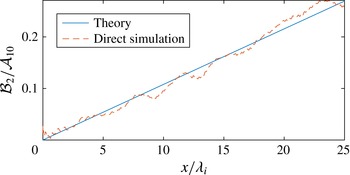
Comparison of analytical results (4.2) with the direct simulation. The physical parameters used are: density gradient $a=1\times 10^{-3}~\text{m}^{-1}$ , water depth $h=100~\text{m}$ , dimensionless wavenumber $kh=3.147946$ , dimensionless frequency $\unicode[STIX]{x1D714}/N=0.4472136$ , the amplitude of vertical velocity of the incident wave $A_{10}=0.1~\text{m}~\text{s}^{-1}$ .

Here we consider propagation of waves in a stratified water of density gradient $a=1\times 10^{-3}~\text{m}^{-1}$ (i.e.  $N=0.1~\text{rad}~\text{s}^{-1}$ ), depth 100 m and in a domain of horizontal extent 20 km. We choose $5\times 10^{3}$ grid points in the $x$ direction and 100 layers in the $z$ direction. We specify the velocity of fluid particles at the left boundary to match that of desired incoming wave. Therefore the left boundary that serves as the incoming wave boundary (wave maker). The right boundary is closed and a slip-free boundary condition is applied. We consider the case of an incident internal wave of mode 2 ( $kh=3.147946$ , $\unicode[STIX]{x1D714}/N=0.4472136$ vertical velocity amplitude $w=0.1~\text{m}~\text{s}^{-1}$ ) with its second harmonic being a mode-1 wave. The time step $\unicode[STIX]{x1D6FF}t/T=1/35000$ where $T$ is the period of the incident wave. We run the simulation until the incident wave arrives at the wall, at which point the amplitude of both waves (incident and its second harmonics) have reached a steady state in the domain of interest $0<x/\unicode[STIX]{x1D706}_{i}<20$ . As is seen from figure 4, the curve of ${\mathcal{B}}_{2}/{\mathcal{A}}_{10}$ vs $x/\unicode[STIX]{x1D706}_{1}$ gives an initial slope of 0.0107 which is the same as our theoretical prediction (4.2).

Figure 5.

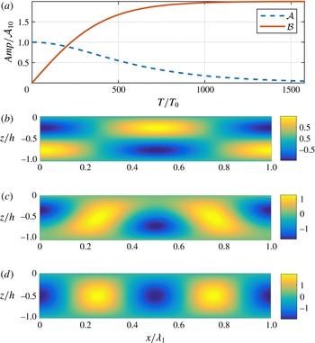
Time evolution of the vertical velocities of internal gravity waves that satisfy the conditions of harmonic generation. The physical parameters used here correspond to figure 3(a). (a) Time evolution of the amplitudes of the two waves. $T_{0}$ is the period of the parent wave. (b–d) Snapshots of the wave field at $t=0$ (b), $t=500T_{0}$ (c) and $1500T_{0}$ (d). The presented mechanism initially results in a modulation of the primary wave, and eventually all the energy goes to the second harmonic.

Figure 6.

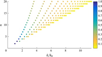
Dependence of the decay rate $R=\sqrt{-\unicode[STIX]{x1D6FC}_{t}\unicode[STIX]{x1D6FD}_{t}}$ on mode numbers $n$ and the horizontal wavenumbers. We normalize the quantities by the wave where the largest decay rate is obtained (here it corresponds to point ‘a’ in figure 1). Colour scale represents $R/R_{0}$ where $R_{0}=3.81\times 10^{-6}~\text{m}^{-1}$ . The physical parameters used here are the same as in figure 1.

To see how fast this instability evolves temporally, we present in figure 5 results of the temporal evolution of the parent wave and its second harmonic, with the same physical parameters as in the case in figure 3(a). The governing equation takes a similar form to (4.2) except the derivatives that are with respect to the time $t$ and clearly expressions for $\unicode[STIX]{x1D6FC}$ and $\unicode[STIX]{x1D6FD}$ are different. The qualitative trend is as the spatial case, and the figure suggests that we need time ${\sim}O(1000)$ times the period of the initial wave to see the majority of the energy transmitted to the second harmonic. With the chosen Brunt–Väisälä frequency of $N=0.022~\text{s}^{-1}$ (correspondingly, the wavenumber is $k=3.14\times 10^{-3}~\text{m}^{-1}$ , the frequency is $9.90\times 10^{-3}~\text{s}^{-1}$ , the wave amplitude is 1 m, the water depth is 1000 m and $a=5\times 10^{-5}~\text{m}^{-1}$ ), the time scale is approximately 10 days, which is of the same order as that of parametric subharmonic instability of the M2 internal tide ( ${\sim}$ 2–5 days) (cf. e.g. MacKinnon & Winters Reference MacKinnon and Winters2005; Gerkema, Staquet & Bouruet-Aubertot Reference Gerkema, Staquet and Bouruet-Aubertot2006). This is somewhat expected as both mechanisms are second-order resonance instabilities. Similar to the spatial case, the governing equation is,

(4.5a ) $$\begin{eqnarray}\displaystyle & \displaystyle \frac{\text{d}{\mathcal{B}}_{2}(t_{1})}{\text{d}t}=\unicode[STIX]{x1D6FC}_{t}{\mathcal{A}}_{1}^{2}(t_{1}), & \displaystyle\end{eqnarray}$$

(4.5b ) $$\begin{eqnarray}\displaystyle & \displaystyle \frac{\text{d}{\mathcal{A}}_{1}(t_{1})}{\text{d}t}=\unicode[STIX]{x1D6FD}_{t}{\mathcal{A}}_{1}(t_{1}){\mathcal{B}}_{2}(t_{1}), & \displaystyle\end{eqnarray}$$

(4.6) $$\begin{eqnarray}\displaystyle \unicode[STIX]{x1D6FC}_{t}=-\frac{3\unicode[STIX]{x1D714}^{2}m_{1}^{2}m_{2}^{2}\cos m_{2}h}{gk^{2}[m_{2}^{3}h+4m_{2}hk^{2}+(m_{2}^{2}-4k^{2})\sin m_{2}h\cos m_{2}h]}, & & \displaystyle\end{eqnarray}$$

(4.7) $$\begin{eqnarray}\displaystyle & \displaystyle \unicode[STIX]{x1D6FD}_{t}=-\frac{m_{1}\sin m_{2}h[(3m_{1}^{2}+m_{2}^{2}+3k^{2})\cos ^{2}m_{1}h-2m_{1}m_{2}\cot m_{2}h\sin 2m_{1}h-(2m_{1}^{2}+m_{2}^{2}+3k^{2})]}{2[2m_{1}^{3}h+2m_{1}hk^{2}+(m_{1}^{2}-k^{2})\sin 2m_{1}h]}. & \displaystyle \nonumber\\ \displaystyle & & \displaystyle\end{eqnarray}$$

The analytical solutions to (4.5) read,

(4.8a ) $$\begin{eqnarray}\displaystyle & \displaystyle {\mathcal{A}}_{1}=A_{10}\text{sech}(A_{10}\sqrt{-\unicode[STIX]{x1D6FC}_{t}\unicode[STIX]{x1D6FD}_{t}}t), & \displaystyle\end{eqnarray}$$

(4.8b ) $$\begin{eqnarray}\displaystyle & \displaystyle {\mathcal{B}}_{2}=-\frac{A_{10}\sqrt{-\unicode[STIX]{x1D6FC}_{t}\unicode[STIX]{x1D6FD}_{t}}\tanh (A_{10}\sqrt{-\unicode[STIX]{x1D6FC}_{t}\unicode[STIX]{x1D6FD}_{t}}t)}{\unicode[STIX]{x1D6FD}_{t}}, & \displaystyle\end{eqnarray}$$

$A_{10}={\mathcal{A}}_{1}(t=0)$

${\mathcal{A}}_{1}$

$3.69/(A_{10}\sqrt{-\unicode[STIX]{x1D6FC}_{t}\unicode[STIX]{x1D6FD}_{t}})$

${\mathcal{A}}_{1}$

$R=\sqrt{-\unicode[STIX]{x1D6FC}_{t}\unicode[STIX]{x1D6FD}_{t}}$

$A_{10}\sqrt{-\unicode[STIX]{x1D6FC}_{t}\unicode[STIX]{x1D6FD}_{t}}$

$n$

We would like to comment here that parametric subharmonic instability (PSI) is dependent upon perturbation waves in the domain in order to get started (Davis & Acrivos Reference Davis and Acrivos1967; Muller Reference Muller1986). For a monochromatic standing wave that is not an exact solution to the fully nonlinear governing equation, for PSI to occur, perturbations are still required since otherwise no subharmonic waves would be excited (see e.g. p. 436 McEwan Reference McEwan1971). In direct simulations, this is achieved by adding random noise to the simulation domain. In experimental studies the required noise already exists in the domain due to unavoidable imperfections. Hence, usually in experiments PSI is automatically obtained (similar to inevitable Benjamin–Feir instability) and destabilizes ‘single’ internal waves to a number of other subharmonic waves (e.g. Martin et al. Reference Martin, Simmons and Wunsch1972). We would like to emphasize that the underlying mechanism of resonant harmonic generation studied here is different than that of PSI in that the former mechanism, among other characteristics, is an ‘inherent’ instability that does not require ambient perturbations to get started.

Three snapshots of the overall vertical velocity $w$ are shown in figure 5(b–d) that highlights the horizontal and vertical structures of the wave field at different times. Energy goes from the original internal wave (b) slowly to its higher harmonics, first leading to modulation of the original wave (c), but eventually the entire energy is at the second harmonic (d) whose frequency and horizontal wavenumber are double the horizontal frequency and wavenumber of the initial wave. The interaction is only between the initial wave and its second harmonic, and no cascading to different waves ensues.

Figure 7.

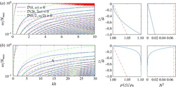
Plots of ${\mathcal{D}}(k,\unicode[STIX]{x1D714})=0$ , ${\mathcal{D}}(2k,2\unicode[STIX]{x1D714})=0$ and ${\mathcal{D}}(k/2,\unicode[STIX]{x1D714}/2)=0$ for parabolic and exponential density profiles (cf. figure 1): (a) for $\unicode[STIX]{x1D70C}(z)=\unicode[STIX]{x1D70C}_{0}(1+az^{2})$ with $a=1\times 10^{-5}~\text{m}^{-2}$ and (b) for $\unicode[STIX]{x1D70C}(z)=\unicode[STIX]{x1D70C}_{0}[1+\unicode[STIX]{x1D6FF}-\unicode[STIX]{x1D6FF}\exp (az)]$ with $a=0.1~\text{m}^{-1}$ and $\unicode[STIX]{x1D6FF}=0.1$ . On the right-side of each plot, we show the normalized density profile $\unicode[STIX]{x1D70C}(z)/\unicode[STIX]{x1D70C}_{0}$ and the Brunt–Väisälä frequency $N(z)^{2}$ of the two nonlinear density profiles (blue solid lines) overlaid of top of corresponding plots of linear density profile (red dashed lines). Water depth is $h=100~\text{m}$ .

We would like to note that the harmonic-generation mechanism proposed here occurs for non-uniformly stratified ocean as well. As pointed out previously, a necessary condition for this to occur is that for a given wave of frequency $\unicode[STIX]{x1D714}$ and wavenumber $k$ , the two conditions ${\mathcal{D}}(k,\unicode[STIX]{x1D714})=0$ and ${\mathcal{D}}(2k,2\unicode[STIX]{x1D714})=0$ are satisfied. We present two examples in figure 7 for two different density profiles: parabolic $\unicode[STIX]{x1D70C}(z)=\unicode[STIX]{x1D70C}_{0}(1+az^{2})$ , where $a=1\times 10^{-5}~\text{m}^{-2}$ (figure 7 a) and exponential $\unicode[STIX]{x1D70C}(z)=\unicode[STIX]{x1D70C}_{0}[1+\unicode[STIX]{x1D6FF}-\unicode[STIX]{x1D6FF}\exp (az)]$ , where $a=0.1~\text{m}^{-1},\unicode[STIX]{x1D6FF}=0.1$ (figure 7 b). The water depth is 100 m for both. The Brunt–Väisälä frequencies increase with depth in one case and decrease in the other. It can been seen from figure 7 that there are, as well, infinitely countable intersections (i.e. solutions) between the two sets of curves. In these cases, contrary to the constant $N$ case, the linear wave solution does not satisfy the nonlinear Boussinesq–Euler equation and hence inclusion of the nonlinear free surface condition is not necessary for the harmonic generation to appear. The analysis for these two cases can be carried out by following the same logic presented in appendix A, although mathematically more involved and closed-form explicit solutions will be tedious, if not impossible, to obtain.

As discussed above, when density profile is not uniform and hence $N$ is not constant, two sources contribute to the harmonic generation: (i) nonlinearities in the free surface boundary condition, i.e. right-hand side of equation (A 8b ) and (ii) nonlinear terms in the momentum equation, i.e. right-hand side of equation (A 8a ). As presented before, for a constant $N$ case the latter source is absent. For non-uniform stratifications, it is of interest to evaluate the relative importance of these two contributors. The motivation is to see whether the classical rigid-lid assumption would be a good approximation in estimating energy exchange due to harmonic generation when the density profile is non-uniform.

We comment on this question briefly by considering the exponential density profile as it is representative of actual pycnoclines. For such a density profile, the vertical structure of an internal wave $W(z)$ is obtained as

(4.9) $$\begin{eqnarray}\displaystyle W(z)=-\frac{J_{\unicode[STIX]{x1D708}}(\unicode[STIX]{x1D707})Y_{\unicode[STIX]{x1D708}}(p)-Y_{\unicode[STIX]{x1D708}}(\unicode[STIX]{x1D707})J_{\unicode[STIX]{x1D708}}(p)}{Y_{\unicode[STIX]{x1D708}}(\unicode[STIX]{x1D707})}, & & \displaystyle\end{eqnarray}$$

where, $J$ and $Y$ are Bessel function of the first and the second kind respectively, and

(4.10a-c ) $$\begin{eqnarray}\displaystyle \unicode[STIX]{x1D708}=\frac{2k}{a},\quad \unicode[STIX]{x1D707}=\frac{2k\sqrt{g\unicode[STIX]{x1D6FF}}\text{e}^{-1/2ah}}{\unicode[STIX]{x1D714}\sqrt{a}},\quad p=\frac{2k\sqrt{g\unicode[STIX]{x1D6FF}}\text{e}^{1/2az}}{\unicode[STIX]{x1D714}\sqrt{a}}. & & \displaystyle\end{eqnarray}$$

By substituting this equation into the right-hand side of equations (A 8a ) and (A 8b ) the relative importance of the right-hand side of the two equations are obtained.

We consider a wave with the wavenumber and frequency $kh=14.14$ and $\unicode[STIX]{x1D714}/N_{max}=0.30$ corresponding to the point highlighted by the character ‘A’ in figure 7(b). Averaged over the $z$ direction, the relative magnitude of nonlinear terms on the right-hand side of the Boussinesq–Euler equation to those of free surface boundary condition (i.e. (A 8a ) to (A 8b )) is only approximately 5 %. This stresses that even in the case of a nonlinear density stratification, the amplitude of nonlinear free surface terms is still much higher (here more than an order of magnitude) than those arising from the nonlinearity of the density profile. It is to be noted that in the nonlinear cases studied in figure 7, Brunt–Väisälä frequencies are significantly different from the linear case. Specifically, in both nonlinear cases, $N$ reaches zero whereas in the linear case $N$ is constant. Clearly the effect of a nonlinear density profile is increased as the profile departs further from a linear one.

We also would like to emphasize that the resonant harmonic generation studied here is different from non-resonant harmonic generation that occurs in non-uniform stratifications (e.g. Sutherland Reference Sutherland2016). The former occurs for specific internal waves, transfers the entire energy to the second harmonic and is a one-way process, whereas the latter obtains for all internal waves but since it is non-resonant only transfers a portion of energy from the initial wave to the superharmonics.

We also would like to note that non-Boussinesq effects (and corresponding terms in the governing equation) can also lead to the generation of resonant super harmonics. In other words, harmonic generation can be obtained in uniform stratification with the rigid lid, if non-Boussinesq terms are not neglected. However, as will be shown shortly, the relative importance of such routing of energy is orders of magnitude less than that of nonlinear free surface avenue: following the same procedure for getting (A 2), except not making Boussinesq approximation, we obtain,

(4.11) $$\begin{eqnarray}\displaystyle & & \displaystyle \unicode[STIX]{x1D70C}\frac{\unicode[STIX]{x2202}}{\unicode[STIX]{x2202}t}\unicode[STIX]{x1D6FB}^{2}w+\unicode[STIX]{x1D70C}\unicode[STIX]{x1D6FB}_{H}^{2}(\boldsymbol{u}\boldsymbol{\cdot }\unicode[STIX]{x1D735}w)-\unicode[STIX]{x1D70C}\frac{\unicode[STIX]{x2202}^{2}}{\unicode[STIX]{x2202}x\unicode[STIX]{x2202}z}(\boldsymbol{u}\boldsymbol{\cdot }\unicode[STIX]{x1D735}u)-\unicode[STIX]{x1D70C}\frac{\unicode[STIX]{x2202}^{2}}{\unicode[STIX]{x2202}y\unicode[STIX]{x2202}z}(\boldsymbol{u}\boldsymbol{\cdot }\unicode[STIX]{x1D735}v)+g\unicode[STIX]{x1D6FB}_{H}^{2}\unicode[STIX]{x1D70C}\nonumber\\ \displaystyle & & \displaystyle \quad +\,2\unicode[STIX]{x1D735}\unicode[STIX]{x1D70C}\boldsymbol{\cdot }\unicode[STIX]{x1D735}\frac{\unicode[STIX]{x2202}w}{\unicode[STIX]{x2202}t}+\frac{\unicode[STIX]{x2202}w}{\unicode[STIX]{x2202}t}\unicode[STIX]{x1D6FB}^{2}\unicode[STIX]{x1D70C}+2\unicode[STIX]{x1D735}\unicode[STIX]{x1D70C}\boldsymbol{\cdot }\unicode[STIX]{x1D735}(\boldsymbol{u}\boldsymbol{\cdot }\unicode[STIX]{x1D735}w)+\unicode[STIX]{x1D6FB}^{2}\unicode[STIX]{x1D70C}\boldsymbol{\cdot }(\boldsymbol{u}\boldsymbol{\cdot }\unicode[STIX]{x1D735}w)-\frac{\unicode[STIX]{x2202}}{\unicode[STIX]{x2202}z}\left(\frac{\unicode[STIX]{x2202}\boldsymbol{u}}{\unicode[STIX]{x2202}t}\boldsymbol{\cdot }\unicode[STIX]{x1D735}\unicode[STIX]{x1D70C}\right)\nonumber\\ \displaystyle & & \displaystyle \quad -\,\frac{\unicode[STIX]{x2202}}{\unicode[STIX]{x2202}z}[\unicode[STIX]{x1D735}\unicode[STIX]{x1D70C}\boldsymbol{\cdot }(\boldsymbol{u}\boldsymbol{\cdot }\unicode[STIX]{x1D735}\boldsymbol{u})]-\frac{\unicode[STIX]{x2202}}{\unicode[STIX]{x2202}z}\left(\frac{\unicode[STIX]{x2202}\boldsymbol{u}}{\unicode[STIX]{x2202}t}\boldsymbol{\cdot }\unicode[STIX]{x1D735}\unicode[STIX]{x1D70C}\right)=0.\end{eqnarray}$$

Comparing the Boussinesq terms in the above equation and the quadratic terms on the free surface boundary condition, i.e. (A 7), we find that their ratio is of the order of $a/k$ . For the two cases presented above, the ratios are less than 1.6 %.

The harmonic generation through a nonlinear free surface involves two energy transfer processes simultaneously, in one process $(k,\unicode[STIX]{x1D714})$ wave loses energy to $(2k,2\unicode[STIX]{x1D714})$ wave and generates the second harmonic; in the other the $(2k,2\unicode[STIX]{x1D714})$ wave forms a triad resonance with $(k,\unicode[STIX]{x1D714})$ wave and sends energy back in an opposite way. The triad resonance condition is clearly satisfied since $2\unicode[STIX]{x1D714}-\unicode[STIX]{x1D714}=\unicode[STIX]{x1D714}$ and $2k-k=k$ . If at the initial moment we only have $(k,\unicode[STIX]{x1D714})$ wave (i.e. no second harmonic in the domain) then harmonic generation triumphs over triad resonance in transferring energy, resulting in the combined effect that energy only goes in one direction. But it can be shown that there are initial conditions under which the energy at first goes from $(2k,2\unicode[STIX]{x1D714})$ wave to the $(k,\unicode[STIX]{x1D714})$ wave, but even in that case eventually the entire energy is transferred to the $(2k,2\unicode[STIX]{x1D714})$ wave. This can be shown rigorously through Lyapunov stability theorem. Basically, the objective is to prove that ${\mathcal{A}}_{1}=0$ and ${\mathcal{B}}_{2}$ reaching its maximum is the asymptotically stable solution of the dynamical system described by equation (4.2).

To prove this, we first note that (4.2) can be put in the following form

(4.12) $$\begin{eqnarray}\displaystyle \frac{\text{d}}{\text{d}x}\left({\mathcal{B}}_{2}^{2}-\frac{\unicode[STIX]{x1D6FC}}{\unicode[STIX]{x1D6FD}}{\mathcal{A}}_{1}^{2}\right)=0. & & \displaystyle\end{eqnarray}$$

Therefore, since $\unicode[STIX]{x1D6FC}/\unicode[STIX]{x1D6FD}$ can be shown to be always negative (see appendix B), we have

(4.13) $$\begin{eqnarray}\displaystyle {\mathcal{B}}_{2}^{2}-\frac{\unicode[STIX]{x1D6FC}}{\unicode[STIX]{x1D6FD}}{\mathcal{A}}_{1}^{2}={\mathcal{G}}^{2}, & & \displaystyle\end{eqnarray}$$

where ${\mathcal{G}}$ is a constant that is determined by the initial conditions. Equation (4.13) shows that $({\mathcal{A}}_{1},{\mathcal{B}}_{2})$ are always moving on an ellipse. If we define a Lyapunov function $V({\mathcal{A}}_{1})={\mathcal{G}}-\unicode[STIX]{x1D6FC}/|\unicode[STIX]{x1D6FC}|[\int _{0}^{x}\unicode[STIX]{x1D6FC}{\mathcal{A}}_{1}(x)^{2}\,\text{d}x+{\mathcal{B}}_{2}(0)]$ , we find that $V({\mathcal{A}}_{1})\geqslant 0$ and $\text{d}V/\text{d}x<0$ . According to Lyapunov asymptotic stability theorem, the solution of the system converges to ${\mathcal{A}}_{1}=0$ from any starting points as $x$ goes to $\infty$ .