1. Introduction
In nonarchimedean geometry, one of the most basic geometric invariants from real geometry, namely the number of connected components of a set, becomes meaningless. The main aim of this paper is to provide a substitute for this number: to each definable set
 $X$
in a (suitable) nonarchimedean context, we associate an invariant
 $V_0(X)$
. The invariant
 $V_0(X)$
is not just a natural number, but contains some additional geometric information: it is a constant motivic function (which can be specialized to a natural number). A second aim is to introduce a partial preorder
 $\preccurlyeq$
on the set of constructible motivic functions that, in the context of our motivic
 $V_0$
, serves as a replacement for the usual order on the reals (the partial preorder from [Reference Cluckers and LoeserCL08] would not be suited for this purpose).
To illustrate how
 $V_0$
and
 $\preccurlyeq$
allow new insights towards a consistent motivic integral geometry theory, we give several practical applications. Indeed, in the nonarchimedean context, from
 $V_0$
we define the counterpart of classical real integral geometry invariants, the Vitushkin variations
 $V_i$
, and we prove the counterpart of celebrated formulas in real integral geometry, the Cauchy–Crofton formula, based on
 $V_0$
, and the Ivanov formula for the metric entropy, based on the
 $V_i$
and
 $\preccurlyeq$
.
In order to explain in detail why and how we develop this program, we begin in this introduction with a presentation of the real geometric context.
In singularity theory, invariants defined through a deformation process and additive invariants (or maps) are ubiquitous. Archetypical instances of such constructions are the Milnor fibre in singularity theory and the Lipschitz–Killing curvatures in differential or integral geometry.
The Milnor number of a polynomial function germ
 $f\colon (\mathbb {C}^n,0)\to (\mathbb {C},0)$
having an isolated singularity at
 $0$
may be defined (up to sign and shift by
 $1$
) as the Euler characteristic
 $\chi$
of the nearby fibre
 $\{f=\varepsilon \}\cap B(0,\eta )$
, for
 $0\lt \varepsilon \ll \eta \ll 1$
. Here, the nearby fibre
 $\{f=\varepsilon \}$
is viewed as a deformation of the singular fibre
 $\{f=0\}$
. The Milnor number counts the cycles of real dimension
 $n-1$
in
 $\{f=\varepsilon \}\cap B(0,\eta )$
that vanish at the singular fibre
 $f=0$
.
For
 $X$
a compact subset of
 $\mathbb {R}^n$
definable in a given o-minimal structure expanding the real field, the Lipschitz–Killing curvatures of
 $X$
are defined through the deformation of
 $X$
by the family
 $(T_\varepsilon )_{\varepsilon \gt 0}$
of its tubular neighbourhoods
 \begin{equation*} T_\varepsilon (X) :=\{x\in \mathbb {R}^n; \mathrm {dist}(x,X)\le \varepsilon \}, \end{equation*}
and through the modified volume
 $\mathcal {V}_\varepsilon (X)$
of
 $T_\varepsilon (X)$
, defined by
 \begin{equation} \mathcal {V}_\varepsilon (X)=\int _{x\in T_\varepsilon (X)} \chi (B(x,\varepsilon )\cap X) \ \mathrm {d}x. \end{equation}
Note that in case
 $X$
is smooth and compact, for
 $\varepsilon$
small enough,
 $\mathcal {V}_\varepsilon (X)=\mathrm {Vol}_n(T_\varepsilon (X))$
, since
 $\chi (B(x,\varepsilon )\cap X)=1$
for any
 $\varepsilon \gt 0$
small enough. Strikingly, it turns out that
 $\mathcal {V}_\varepsilon (X)$
is a polynomial in
 $\varepsilon$
, i.e.
 \begin{equation} \mathcal {V}_\varepsilon (X)=\sum _{i=0}^n \alpha _i \Lambda _{n-i}(X) \varepsilon ^i, \end{equation}
with universal coefficients
 $\alpha _i$
depending only on
 $i$
, and coefficients
 $\Lambda _i(X)$
depending only on
 $X$
. Those
 $\Lambda _i(X)$
are called the Lipschitz–Killing curvatures of
 $X$
(see, for instance, [Reference Bernig and BröckerBB02, Reference FuFu85] for the definable case, and [Reference WeylWey39] for the smooth case). On the other hand, the
 $\Lambda _i(X)$
are also defined by the integral formula
 \begin{equation} \forall i=0, \ldots, n, \quad \Lambda _i(X)=\beta (i,n)\int _{\bar P\in \bar {\operatorname {G}}_n^{n-i}} \chi (X\cap \bar P ) \ \mathrm {d}\bar P, \end{equation}
where
 $ \bar {\operatorname {G}}_n^{n-i}$
is the Grassmannian of
 $(n-i)$
-dimensional affine subspaces of
 $\mathbb {R}^n$
and
 $\beta (i,n)$
is a universal constant depending only on
 $i$
and
 $n$
(see [Reference ComteCom15] for a survey on this question).
A way to modify the Lipschitz–Killing curvature is to replace in formula (3) the additive Euler characteristic
 $\chi$
by the sub-additive number of connected components
 $V_0$
. In this way, one obtains a new sequence of invariants
 $V_0(X), \ldots, V_n(X)$
attached to
 $X$
, called the Vitushin variations (see, for instance, [Reference IvanovIva75, Reference VituškinVit55] and [Reference Yomdin and ComteYC04, Chapter 3])
 \begin{equation} \forall i=0, \ldots, n, \quad V_i(X)=\beta (i,n)\int _{\bar P\in \bar {\operatorname {G}}_n^{n-i} } V_0 (X\cap \bar P ) \ \mathrm {d}\bar P. \end{equation}
Note that directly from equality (4), one obtains
 $V_n(X)=\mathrm {Vol}_n(X)$
. It is a remarkable fact that when
 $\Lambda _i$
is replaced by
 $V_i$
, (using
 $V_0$
instead of
 $\chi$
in (3)), the sequence
 $V_0(X), \ldots, V_n(X)$
is still related to the volume of
 $T_\varepsilon (X)$
by the notion of metric entropy
 $M(\varepsilon,X)$
of
 $X$
, defined as the minimal number of balls of radius
 $\varepsilon \gt 0$
needed to cover
 $X$
. Indeed, a relation between the metric entropy and the variations of
 $X$
, comparable to (2), holds, but here, instead of having an equality, we only have a bound from above for
 $M(\varepsilon,X)$
, due to the fact that
 $\chi$
has been replaced by the looser invariant
 $V_0$
:
 \begin{equation} \forall \varepsilon \gt 0, \quad M(\varepsilon, X)\le C(n)\sum _{i=0}^n \frac {1}{\varepsilon ^i}V_i(X), \end{equation}
where
 $C(n)$
is a constant depending only on
 $n$
(see [Reference IvanovIva75] and [Reference Yomdin and ComteYC04, Theorem 3.5]).
To prove (5), one introduces relative variations
 $V_i(X,B)$
of
 $X$
, where
 $B$
is some ball. For this, one first defines
 $V_0(X,B)$
as the number of connected components of
 $X$
strictly lying in
 $B$
and then defines
 $V_1(X,B), \ldots, V_n(X,B)$
by
 \begin{equation} \forall i=0, \ldots, n, \quad V_i(X,B)=\beta (i,n)\int _{\bar P\in \bar {\operatorname {G}}_n^{n-i} } V_0(X\cap \bar P, B) \ \mathrm {d}\bar P. \end{equation}
With this notation, inequality (5) is a consequence of
 \begin{equation} \sum _{i=0}^n V_i(X,B_1)\ge c(n), \end{equation}
for a constant
 $c(n)$
depending only on
 $n$
and for any unit ball
 $B_1$
centred at a point of
 $X$
(see [Reference IvanovIva75, Theorem II.5.1], [Reference Yomdin and ComteYC04, Theorem 3.4] and [Reference ZernerZer70, Theorem 2] for a proof of (7)).
Inequality (7) says that the relative Vitushkin variations of
 $X$
in the unit ball
 $B_1$
cannot all be simultaneously too small. If
 $X$
has a connected component strictly included in
 $B_1$
, then indeed, the sum of the
 $V_i(X,B_1)$
is at least
 $1$
since
 $V_0(X,B_1)\ge 1$
. Otherwise, the connected component of
 $X$
containing the centre of
 $B_1$
reaches the boundary of
 $B_1$
, and this then yields that at least one relative variation
 $V_i(X,B_1)$
,
 $i\ge 1$
, is big. For instance, in the situation
 $\dim (X)=1$
, a curve connecting the centre of
 $B_1$
and its boundary certainly lies in
 $X$
, and
 $V_1(X,B_1)\ge V_1(R,B_1)=1$
, where
 $R$
is a radius of
 $B_1$
.
In the definable nonarchimedean setting, the notion of deformation is also central. For instance, the notion of motivic Milnor fibre is defined using the rationality of a formal Poincaré series whose coefficients are based on a deformation of the singular fibre. The fact that such a Poincaré series is a rational function shows that in this deformation process, some periodicity phenomenon and therefore some regularity is involved. Note the analogy to the polynomial formulas (2) and (5), which also attest a moderation of the deformation process, viewed from the invariants
 $\Lambda _i(X)$
and
 $V_i(X)$
. Moreover, in the rational form of the Poincaré series series, one can read some geometric data of the germ from which we start, namely (at least) its Milnor number.
This general principle may be illustrated in the specific framework of this paper, where the question of the existence of invariants related to the family of tubular neighbourhoods is addressed. For this, let us fix a complete equi-characteristic
 $0$
valued field
 $K$
with value group
 $ \mathbb {Z}$
, and let us consider the definable family of tubular neighbourhoods
 $ (T_r(X))_{r \in \mathbb {N}}$
of a definable subset
 $X$
of the unit ball of
 $K^n$
, namely,
 \begin{equation*} T_r(X):=\{y\in K^n ; \exists x\in X, \mathrm {val}(y-x)\ge r)\}. \end{equation*}
By [Reference Cluckers and LoeserCL08, Theorem 14.4.1], the formal Poincaré series of the motivic volumes of this family is rational (see § 3 for notation):
 \begin{equation*} \sum _{r\in \mathbb {N}} \mu _n(T_r(X))T^r \in \mathcal {C}(\{pt\}) [\![ T ]\!]_M, \end{equation*}
where
 $\mathcal {C}(\{pt\}) [\![ T ]\!]_M$
is the algebra of polynomials in
 $T$
with coefficients in
 $\mathcal {Q}(\{pt\})\otimes _{\mathbb {Z}[\mathbb {L}-1]} A$
(see Notation 4.1) localized by the multiplicative set
 $M$
generated by polynomials
 $1-\mathbb {L}^\alpha T^\beta$
,
 $\alpha \in \mathbb {Z}, \beta \in \mathbb {N}\setminus \{0\}$
. In particular, considering a generator
 ${P_k(T)}/{(1-\mathbb {L}^{\alpha _k} T^{\beta _k})^k}$
of
 $\mathcal {C}_{\{pt\}} [\![ T ]\!]_M$
, its Taylor formula shows that it contributes to the series only for coefficients of order
 $r=p+m\beta _k$
,
 $m\in \mathbb {N}$
, where
 $p$
runs over the degrees of the monomials appearing in
 $P_k$
. Moreover, this contribution has the form
 $\mathbb {L}^{m\alpha _k} Q_k(m)$
with
 $Q_k$
a polynomial with coefficients in
 $\mathcal {Q}({\{pt\}})\otimes _{\mathbb {Z}[\mathbb {L}-1]} A$
. In conclusion, there exist a finite number of functions of
 $r$
,
 $R_1, \ldots, R_\ell$
such that
 \begin{equation} \mu _n(T_r(X))\in \{ R_1(r), \ldots, R_\ell (r) \}, \end{equation}
each
 $R_i$
being a linear combination with coefficients in
 $\mathcal {Q}({\{pt\}})\otimes _{\mathbb {Z}[\mathbb {L}-1]} A$
of elements of the form
 \begin{equation*} C_k\left(\frac {r-p_{k,j}}{\beta _k}\right)\mathbb {L}^{\alpha _k({r-p_{k,j}})/{\beta _k}}, \end{equation*}
where
 $C_k$
are polynomials,
 $p_{k,j}$
range in a finite subset of
 $\mathbb {N}$
,
 $\alpha _k\in \mathbb {Z}$
,
 $ \beta _k\in \mathbb {N}$
, with the condition that
 $r=p_{k,j}\,\text{mod}\, {\beta _k}$
.
The functions
 $R_1, \ldots, R_\ell$
encode the arithmetico-logical complexity of the set
 $X$
, but it does not seem that one can easily extract from them some geometrical meaning, in contrast to the case of the Poincaré series defining the motivic Milnor fibre, and in contrast to the smooth or convex real case, where
 $\ell =1$
and
 $R_1$
is a polynomial function of the radius of the tubular neighbourhood, from which the Lipschitz–Killing curvatures appear as coefficients (see (2)). In the tubular deformation family no motivic version of the
 $\Lambda _i$
may clearly be identified, except maybe in the trivial case where
 $X$
is a smooth variety of dimension
 $d$
: in this case only the
 $d$
-volume of
 $X$
appears since one has
 $\mu _n(T_r(X))=\mu _d(X)\mathbb {L}^{-r(n-d)}$
. Note finally that since in the Hrushovski–Kazhdan version of motivic integration [Reference Hrushovski and KazhdanHK06] a notion of motivic Euler characteristic appears, one may think that defining with the latter a motivic modified volume modelled on formula (1) could make it possible to relate it to a motivic version of the
 $\Lambda _i$
, also defined in this context by (3), for instance by a formula comparable to (2). But so far all attempts in this direction have failed.
Nevertheless, in spite of this apparent lack of geometric information in the deformation of
 $X$
via the family of tubular neighbourhoods, we show in § 6 that one can transfer to the nonarchimedean setting the notion of Vitushkin variations, and in § 8 that these motivic Vitushkin variations are this time deeply related to the motivic metric entropy. Indeed, one of the main results of this paper is Theorem 8.9, the nonarchimedean counterpart of inequality (5).
By definition, the motivic metric entropy
 $M(X,r)$
of
 $X$
is the motivic measure (instead of the number in the real situation) of balls one needs to cover
 $X$
(see Definition 8.8). But it turns out in the nonarchimedean setting that
 $M(X,r)$
is also
 $\mu (T_r(X))$
, and thus the family
 $(M(X,r))_{r\in \mathbb {N}}$
is in general expressed in the form given by (8), from which there is a priori no obvious way to identify some convenient geometrical invariants attached to
 $X$
.
The principal obstruction we have to overcome when aiming to find nonarchimedean substitutes of the variations
 $V_i(X)$
is finding a sensible notion of (number of) connected components. For this, we use the notion of riso-triviality introduced in [Reference Bradley-Williams and HalupczokBH22] by Bradley-Williams and the second author (see § 3). Intuitively,
 $V_0$
will be the
 $0$
-dimensional motivic measure of the
 $0$
-dimensional stratum of a (certain kind of) minimal stratification of
 $X$
. While one can think of a t-stratification in the sense of [Reference HalupczokHal14], those may be inherently non-canonical; to obtain a well-defined
 $V_0$
, we use the more abstract approach from [Reference Bradley-Williams and HalupczokBH22] instead.
To define a nonarchimedean version of the relative variation
 $V_0(X, B)$
we also need a replacement for the notion of connected component of
 $X$
lying strictly in
 $B$
. It turns out that we can use the condition that
 $X$
can be stratified in such a way that
 $B$
is disjoint from the
 $0$
-dimensional stratum. For the accurate definition of the nonarchimedean version
 $V_0$
, see Definitions 6.1 and 8.2.
Another technical difficulty to establish the nonarchimedean version of inequality (5) or (7) is the following. Since
 $V_0(X)$
is defined as the
 $0$
-dimensional motivic measure of some definable set in the valued field, we have to introduce in § 5 a notion of a partial preorder allowing us to compare, for instance, a class in
 $\mathcal {Q}_+({\{pt\}})$
, the Grothendieck semiring of definable sets in the residue field sort, and a constant function with value in
 $\mathbb {Z}$
(typically
 $[x^2-2=0]$
and the constant function of
 $\mathcal {C}_+(\{pt\})$
equal to
 $1$
(see § 4 for the notation). This crucial need explicitly appears in this simple form in the proof of Theorem 8.6. The partial preorder introduced in [Reference Cluckers and LoeserCL08, 12.2], defined via the set of nonnegative constructible motivic functions (see Remark 4.2), is in general not adapted to this goal. Our more flexible notion of partial preorder on the set of integrable constructible motivic functions, denoted
 $\preccurlyeq$
and extending that of [Reference Cluckers and LoeserCL08, 12.2], is introduced in Definition 5.1 and Lemma 5.6, using motivic integration and definable surjections.
With the invariants
 $V_i$
defined through the nonarchimedean invariant
 $V_0$
as in the real case (see Definition 6.7), as well as their relative version
 $V_i(\cdot, B)$
in a ball
 $B$
(see Definition 8.2), and with this partial preorder relation
 $\preccurlyeq$
, we prove in § 6 the nonarchimedean version of inequality (7) (see Theorem 8.6) and finally the nonarchimedean version of inequality (5) (see Theorem 8.9) relating the motivic entropy defined in Definition 8.8 and the motivic Vitushkin variations
 $V_i$
.
It also turns out (see Theorem 7.1) that if
 $X$
is a definable subset of
 $K^n$
of dimension
 $d$
then
 $V_d(X)$
is the motivic
 $d$
-dimensional volume of
 $X$
(up to some universal constant depending only on
 $d$
and
 $n$
). In other words, the motivic Cauchy–Crofton formula involving
 $V_0$
as the nonarchimedean substitute for the real measure counting holds. This application of the construction of
 $V_0$
shows, at least from the geometric motivic measure theory point of view, that the invariant
 $V_0$
is a good substitute of the real number of points. Such a formula in the nonarchimedean context has been obtained in the local case by A. Forey in [Reference ForeyFor21], on the model of the real local Cauchy–Crofton formula previously obtained in [Reference ComteCom00] for the density by the first author. In this paper, we show the classical (global) motivic version of this formula, the proof of which requires a different approach than in the local case.
The nonarchimedean Cauchy–Crofton formula, as well as the nonarchimedean version of inequality (5), may be viewed as a step towards motivic integral geometry formulas in the nonarchimedean context, based on the
 $0$
-degree motivic invariant
 $V_0$
, such as classical kinematic formulas for homogeneous spaces (note that in the framework of characteristic 0 local fields integral geometry tools have recently been developed using
 $p$
-adic integration in [Reference Bürgisser, Kulkarni and LerarioBKL22, Reference Kulkarni and LerarioKL21]). In this direction, our preorder has a role to play, since the absence of a suitable nonarchimedean substitute of the Euler characteristic might make it necessary to replace equalities in classical real formulas involving the Euler characteristic with inequalities involving
 $V_0$
. As explained above, this principle is applied here to the lack of a geometric nonarchimedean version of formula (2), turned into the geometric nonarchimedean version of inequality (5).
2. Language, theory, structure, definable sets
Definition 2.1. Throughout this paper,
 $k$
is a field of characteristic
 $0$
and
 $K := k(\!(t)\!)$
is the field of formal Laurent series. We write
 $\mathcal {O}_K = k[\![t]\!]$
for the valuation ring of
 $K$
,
 $\operatorname {res}\colon \mathcal {O}_K \to k$
for the residue map,
 $\mathrm {ac}\colon K \to k$
for the (natural) angular component map and
 $\mathrm {val}\colon K \to \mathbb {Z} \cup \{\infty \}$
for the valuation map,
 $\mathcal {M}_K=\{ x\in K; \mathrm {val}(x)\gt 0 \}$
, the maximal ideal. We extend the valuation to
 $K^n$
, by setting
 $\mathrm {val}((a_1, \dots, a_n)) := \min _i \mathrm {val}(a_i)$
.
Notation 2.2. We sometimes also use a more intuitive, multiplicative notation for the valuation,
 \begin{equation*} K \to \mathbb {L}^{\mathbb {Z}} \cup \{0\}, \quad a \mapsto |a| := \mathbb {L}^{-\mathrm {val}(a)}, \end{equation*}
and the multiplicative value group
 $\mathbb {L}^{\mathbb {Z}}$
is equipped with the order satisfying
 $\mathbb {L}^r \le \mathbb {L}^s$
if and only if
 $r \le s$
. Note that this notation suggests a natural map from
 $\mathbb {L}^{\mathbb {Z}}$
into the set of constructible motivic functions
 $\mathcal {C}(\{pt\})$
at the point (see Notation 4.1).
Notation 2.3. For
 $x \in K^n$
and
 $\lambda \in \mathbb {L}^{\mathbb {Z}}$
, we write
 \begin{equation*} B(x,\lambda ) = \{y \in K^n; |y - x| \le \lambda \} \end{equation*}
for the closed ball of radius
 $\lambda$
around
 $x$
. By a ball, we mean such a closed valuative ball. We denote the radius
 $\lambda$
of
 $B(x,\lambda )$
by
 $\operatorname {rad} B(x,\lambda )$
.
Throughout this paper, we also fix a language
 $\mathcal {L}$
and consider
 $K$
as an
 $\mathcal {L}$
-structure. One possibility is to take
 $\mathcal {L}$
to be the Denef–Pas language
 $\mathcal {L}_{\mathrm {DP}}$
.
Definition 2.4. The Denef–Pas language
 $\mathcal {L}_{\mathrm {DP}}$
consists of one sort for
 $K$
with the ring language, one sort for
 $k$
with the ring language, one sort for
 $\mathbb {Z}$
(the value group) with the language
 $\{0,+, \lt \}$
of ordered abelian groups, the valuation map and the angular component map.
However, all our results also hold for various other languages
 $\mathcal {L}$
. The following are the assumptions we really need.
Definition 2.5. Let
 $\mathcal {L}$
be an expansion of the language
 $\mathcal {L}_{\mathrm {DP}}$
on
 $K$
with the following properties.
-
(1) The theory
 $\mathrm {Th}_{\mathcal {L}}(K)$
is
$1$
-h-minimal in the sense of [Reference Cluckers, Halupczok and Rideau-KikuchiCHR22].
-
(2) The value group and the residue field are orthogonal (i.e. every definable set
$X \subseteq k^m \times \mathbb {Z}^n$
is a finite union of sets of the form
$Y \times Z$
, for
$Y \subseteq k^m$
and
$Z \subseteq \mathbb {Z}^n)$
. -
(3) The induced structure on
$\mathbb {Z}$
is the pure ordered abelian group structure.


Remark 2.6. All conditions of Definition 2.5 are preserved under adding constants from
 $K$
,
 $k$
or
 $\mathbb {Z}$
, so anything which we prove about
 $\emptyset$
-definable sets and/or maps also holds for
 $A$
-definable sets/maps, when
 $A$
is a subset of
 $K\cup k \cup \mathbb {Z}$
. We will use this implicitly on various occasions.
Instead of imposing
 $K = k(\!(t)\!)$
, one could have allowed
 $K$
to be a Henselian valued field with residue field
 $k$
and value group
 $\mathbb {Z}$
. The reasons not to do that are that (a) if
 $K$
is not spherically complete, the definition of
 $V_0$
becomes more technical and (b) the case
 $K = k(\!(t)\!)$
implies the more general case, as follows.
First note that any such more general
 $K$
can be embedded into its maximal immediate extension, which is isomorphic to
 $k(\!(t)\!)$
, and by [Reference Bradley-Williams and HalupczokBH21], the
 $\mathcal {L}$
-structure on
 $K$
can be extended to
 $k(\!(t)\!)$
in such a way that
 $k(\!(t)\!)$
is an elementary extension of
 $K$
. For that reason, assuming
 $K = k(\!(t)\!)$
is not a restriction, provided that the results we are proving are first-order statements. This is indeed the case for our results in the following sense.
Our definition of
 $V_0$
(Definition 6.1) uses the notion of riso-triviality (Definition 3.3) which, as formulated, is not a first-order condition. Moreover, if
 $K$
is not spherically complete, defined like this, the notion of riso-triviality would lose many of its good properties, rendering it useless for our purposes (see Remark 3.2). We do not know a direct way to fix this, but there is a simple indirect fix. By Theorem 3.7, there exists a formula expressing riso-triviality in every spherically complete field. We simply take that formula as the definition of riso-triviality in non-spherically complete fields, thus making that notion first-order by definition.
With this definition of
 $V_0$
, all our results (in particular, Theorems 7.1, 8.6 and 8.9) also hold in any
 $K \prec k(\!(t)\!)$
. Indeed, those are equalities and inequalities between constructible motivic functions. Any such (in)equality is witnessed by finitely many formulas (e.g., defining some bijections or ingredients of other constructible motivic functions); the witnesses that work in
 $k(\!(t)\!)$
then also work in
 $K$
.
Remark 2.7. [Reference Cluckers, Halupczok and Rideau-KikuchiCHR22, Proposition 2.6.12] states that under the assumption of
 $1$
-h-minimality, the
 $\mathrm {RV}$
-sort (which, in our setting, is just
 $k \times \mathbb {Z}$
) is stably embedded in a strong sense. Combining this with orthogonality of the value group and the residue field, one deduces that the residue field is also stably embedded in that strong sense. One way to formulate this is as follows: if
 $X \subset K^n \times k^m \times \mathbb {Z}^r$
and
 $Z \subseteq X \times k^{m'}$
are
 $\emptyset$
-definable, for some
 $n, m, r, m' \in \mathbb {N}$
, then there exist an
 $m'' \in \mathbb {N}$
, an
 $\emptyset$
-definable map
 $\rho \colon X \to k^{m''}$
and a
 $\emptyset$
-definable set
 $\hat Z \subseteq k^{m''} \times k^{m'}$
such that for every
 $x \in X$
, the fibre
 $Z_x$
is equal to the fibre
 $\hat Z_{\rho (x)}$
. (To get from the version of stable embeddedness of [Reference Cluckers, Halupczok and Rideau-KikuchiCHR22, Proposition 2.6.12] to the one given here, one uses a standard compactness argument: first, one applies stable embeddedness to each fibre
 $Z_x$
individually, and then compactness shows that the resulting
 $\rho (x)$
and
 $\hat Z_{\rho (x)}$
can be taken to be definable uniformly in
 $x$
.)
3. Riso-triviality
In this section we present the notion of riso-triviality defined and studied in [Reference Bradley-Williams and HalupczokBH22], a notion that we use in the rest of the paper. A set
 $X\subseteq K^n$
is said to be riso-trivial on some ball
 $B \subseteq K^n$
if it is roughly translation invariant on
 $B$
, in some directions specified by a sub-vector space
 $V \subseteq k^n$
. Note that many definitions and statements in [Reference Bradley-Williams and HalupczokBH22] speak about riso-triviality of maps
 $\chi$
defined on
 $K^n$
. If one is interested in a set
 $X \subseteq K^n$
, one should take
 $\chi$
to be the indicator function of
 $X$
.
Definition 3.1. A map
 $\Phi \colon X \to Y$
between sets
 $X, Y \subseteq K^n$
is called a risometry if, for every
 $x, x' \in X$
with
 $x \ne x'$
, we have
 \begin{align*}\mathrm {val}((\Phi (x')-\Phi (x))-(x'-x))\gt \mathrm {val}(x'-x). \\[-15pt]\end{align*}
Remark 3.2. Clearly, risometries are always injective. Moreover, in our setting, a risometry from a ball
 $B \subseteq K^n$
to itself is always surjective. Indeed, since
 $K = k(\!(t)\!)$
is spherically complete (meaning that any descending chains of balls have non-empty intersection), surjectivity can be deduced using a version of the Banach fixed point theorem in such fields (see [Reference Bradley-Williams and HalupczokBH22, Lemma 3.3.4]). That surjectivity is crucial for the existence of
 $\mathrm {rtsp}_B$
in Definition 3.3 below.
Definition 3.3 (Riso-triviality on a ball). Suppose that
 $X \subseteq K^n$
is an arbitary set and that
 $B \subseteq K^n$
is a ball.
-
(1) Given a sub-vector space
$V$
of
$k^n$
, we say that
$X$
is V-riso-trivial on B if there exist a lift
$\tilde V \subseteq K^n$
of
$V$
(i.e. satisfying
$\operatorname {res}(\tilde V) = V$
) and a risometry
$\Phi \colon B \to B$
such that
$\Phi ^{-1}(X \cap B)$
is
$\tilde V$
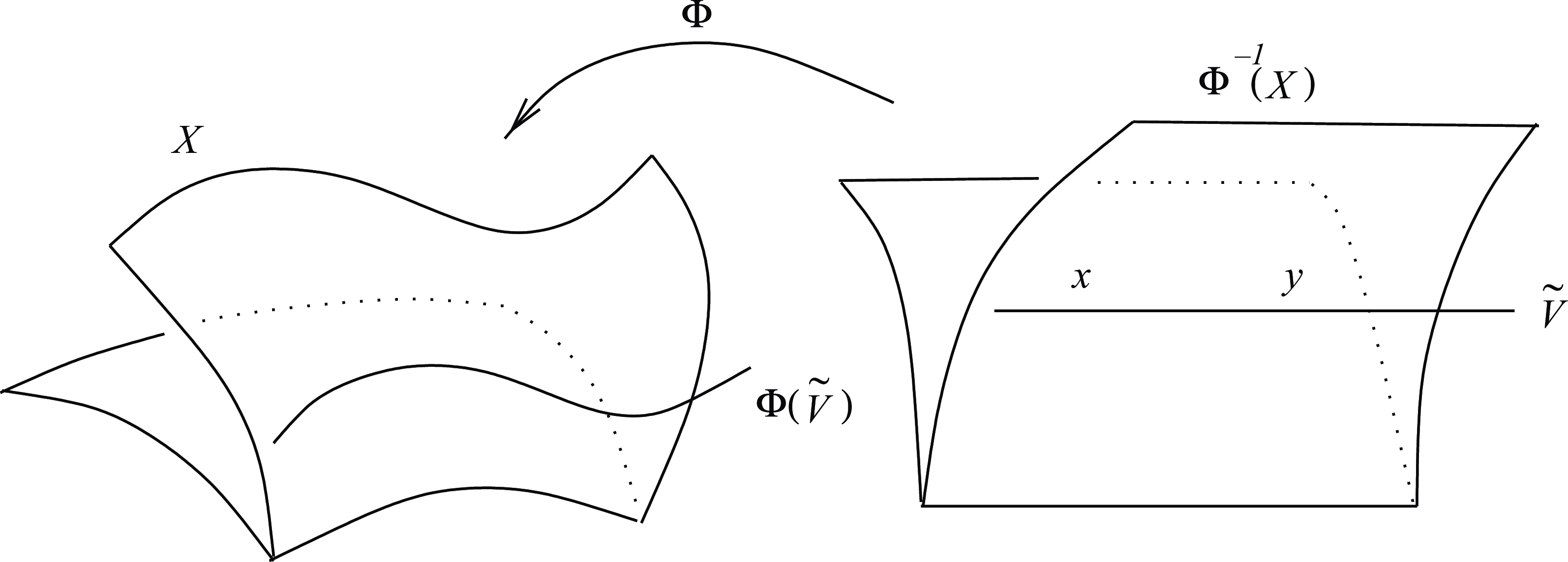
-translation invariant, i.e. for every pair of points
$x,y\in B$
satisfying
$y-x\in \tilde {V}$
, we have (see Figure 1)
\begin{align*} x \in \Phi ^{-1}(X\cap B)\Longleftrightarrow y\in \Phi ^{-1}(X\cap B). \\[-15pt] \end{align*}
-
(2) The riso-triviality space of
$X$
on
$B$
is the maximal (with respect to inclusion) subspace
$V \subseteq k^n$
such that
$X$
is
$V$
-riso-trivial on
$B$
; we denote it by
$\mathrm {rtsp}_B(X)$
. Such a maximal subspace exists by [Reference Bradley-Williams and HalupczokBH22, Proposition 2.3.12]. -
(3) We say that
$X$
is d-riso-trivial on
$B$
if
$\dim \mathrm {rtsp}_B(X) \ge d$
, and we say that it is not riso-trivial if
$X$
is not even
$1$
-riso-trivial. If it is clear which set
$X$
we are talking about, we may also say that
$B$
is
$d$
-riso-trivial, meaning that
$X$
is
$d$
-riso-trivial on
$B$
.


 $1$
-riso-triviality on a ball.

Note that even though the above notions will be applied to definable sets
 $X$
, we do not require the risometry
 $\Phi$
to be definable.
We will apply the above notions also for
 $X$
and
 $B$
living in an affine subspace
 $\bar P \subseteq K^n$
, by identifying
 $\bar P$
with
 $K^{\dim \bar P}$
.
Various good properties of these notions are proved in [Reference Bradley-Williams and HalupczokBH22]. We now recall a few of them.
Remark 3.4. One easily sees that if a set
 $X \subseteq K^n$
is
 $V$
-riso-trivial on a ball
 $B \subseteq K^n$
, for some
 $V \subseteq k^n$
, then
 $X$
is also
 $V'$
-riso-trivial on any sub-ball
 $B' \subseteq B$
for any sub-vector space
 $V' \subseteq V$
.
Remark 3.5. In Definition 3.3(1), the choice of the lift
 $\tilde V$
does not matter, i.e. if there exist a lift and a risometry
 $\Phi$
witnessing
 $V$
-riso-triviality, then for any other lift
 $\tilde V'$
of
 $V$
, there exists a risometry
 $\Phi '$
such that
 $(\tilde V', \Phi ')$
also witness
 $V$
-riso-triviality.
Proposition 3.6 (see [Reference Bradley-Williams and HalupczokBH22, Lemma 3.3.14]). Let
 $X\subseteq K^n$
be a set, let
 $B\subseteq K^n$
be a ball, and set
 $\ell := n - \dim \mathrm {rtsp}_B(X)$
. Fix
 $\bar P$
in the Grassmannian manifold
 $\bar {\operatorname {G}}_n^{\ell }$
of
 $\ell$
-dimensional affine subspaces of
 $K^n$
, such that
 $\bar P \cap B \ne \emptyset$
and such that, if we denote by
 $P \subseteq K^n$
the direction of
 $\bar P$
,
 $\operatorname {res}(P) \cap \mathrm {rtsp}_B(X) = \{0\}$
. Then
 $X \cap \bar P$
is not riso-trivial on
 $B \cap \bar P$
.
The idea of the proof of this proposition is that if
 $X$
were
 $V$
-riso-trivial on
 $B \cap \bar P$
, this would also imply
 $V$
-riso-triviality on
 $B \cap \bar P'$
for all
 $\bar P'$
parallel to
 $\bar P$
and we could deduce
 $(V\oplus \mathrm {rtsp}_B(X))$
-riso-triviality of
 $X$
on
 $B$
.
One of the central results of [Reference Bradley-Williams and HalupczokBH22] is that
 $\mathrm {rtsp}_B(X)$
depends definably on
 $X$
and
 $B$
. More precisely, we have the following statement.
Theorem 3.7 [Reference Bradley-Williams and HalupczokBH22, Corollary 3.1.3]. Suppose we are given a
 $\emptyset$
-definable family
 $(B_z)_{z\in Z}$
of balls
 $B_z\subseteq K^n$
, and a
 $\emptyset$
-definable family
 $(X_{z})_{z\in Z}$
of subsets
 $X_z \subseteq K^n$
, all parametrized by a
 $\emptyset$
-definable set
 $Z$
. Then the map
 \begin{equation*} Z \to \bigcup _d G^d_n(k),\quad z \mapsto \mathrm {rtsp}_{B_z}(X_{z}) \end{equation*}
is
 $\emptyset$
-definable. Moreover, a formula defining that map in
 $K$
also works in any other spherically complete
 $K' \equiv K$
.
Another important ingredient we will need is that one can control precisely on which balls a definable set is not riso-trivial.
Theorem 3.8.
Given a definable set
 $X \subseteq K^n$
, there exist finitely many disjoint sets
 $B_1, \dots, B_\ell \subseteq K^n$
each of which is either a singleton or a ball such that for every ball
 $B \subseteq K^n$
,
 $X$
is not riso-trivial on
 $B$
if and only if
 $B_i \subseteq B$
for some
 $1 \le i \le \ell$
.
Proof.
By [Reference Bradley-Williams and HalupczokBH22, Lemma 3.4.3], the `rigid core’
 $\operatorname {Crig}_X$
is a finite set of pairwise disjoint singletons and balls. By the definition of
 $\operatorname {Crig}_X$
(just before that lemma), we have
 $\operatorname {Crig}_X = $
 $\{B_1, \dots, B_\ell \}$
.
Note that if
 $B$
is a proper sub-ball of some of the
 $B_i$
, then necessarily
 $X$
is
 $1$
-riso-trivial on
 $B$
, since then,
 $B$
contains no
 $B_j$
.
Remark 3.9. The sets
 $B_1, \dots, B_\ell$
are uniquely determined by
 $X$
, up to permutation; these are:
-
(1) those balls
$B$
for which
$X$
is not riso-trivial on
$B$
but
$1$
-riso-trivial on any proper sub-ball of
$B$
; and -
(2) those singletons
$\{b\}$
such that
$X$
is not riso-trivial on every ball containing
$b$
.


Remark 3.10. By Theorem 3.7, the characterization of the
 $B_i$
given in Remark 3.9 is definable: if
 $(X_{z})_{z\in Z}$
is a
 $\emptyset$
-definable familiy of sets
 $X_z \subseteq K^n$
and
 $C_z$
is the union of the points and balls
 $B_{z,1}, \dots, B_{z,\ell _z}$
corresponding to
 $X_z$
, then
 $(C_z)_z$
is also a
 $\emptyset$
-definable family. In addition, for any such family, there exists
 $N \in \mathbb {N}$
bounding the cardinalities
 $\ell _z$
for all
 $z \in Z$
. (This follows by applying [Reference Bradley-Williams and HalupczokBH22, Lemma 3.4.3] in a language with a constant symbol for
 $z$
added.)

Example 3.11. Set
 $X := \mathcal {O}_K \times \{0\} \subset K^2$
. Then clearly
 $X$
is
 $1$
-riso-trivial on
 $\mathcal {O}_K \times \mathcal {O}_K$
but not on
 $B := t^{-1}\mathcal {O}_K \times t^{-1}\mathcal {O}_K$
(recall that
 $t \in \mathcal {O}_K$
is a generator of the maximal ideal of
 $K$
). In this way, one obtains that the finitely many sets
 $B_i$
provided for
 $X$
by Theorem 3.8 consist only of
 $B$
.
Example 3.12. Let
 $X \subset K^2$
be the graph of the function
 $x \mapsto x^2$
. Then one can verify that
 $X$
is not riso-trivial on
 $\mathcal {O}_K \times \mathcal {O}_K$
but
 $1$
-riso-trivial on each proper sub-ball of
 $\mathcal {O}_K \times \mathcal {O}_K$
. This shows that
 $B := \mathcal {O}_K \times \mathcal {O}_K$
is among the balls provided by Theorem 3.8. One then also checks that
 $X$
is
 $1$
-riso-trivial on every ball disjoint from
 $B$
, so
 $B$
is the only ball given by Theorem 3.8 for
 $X$
.
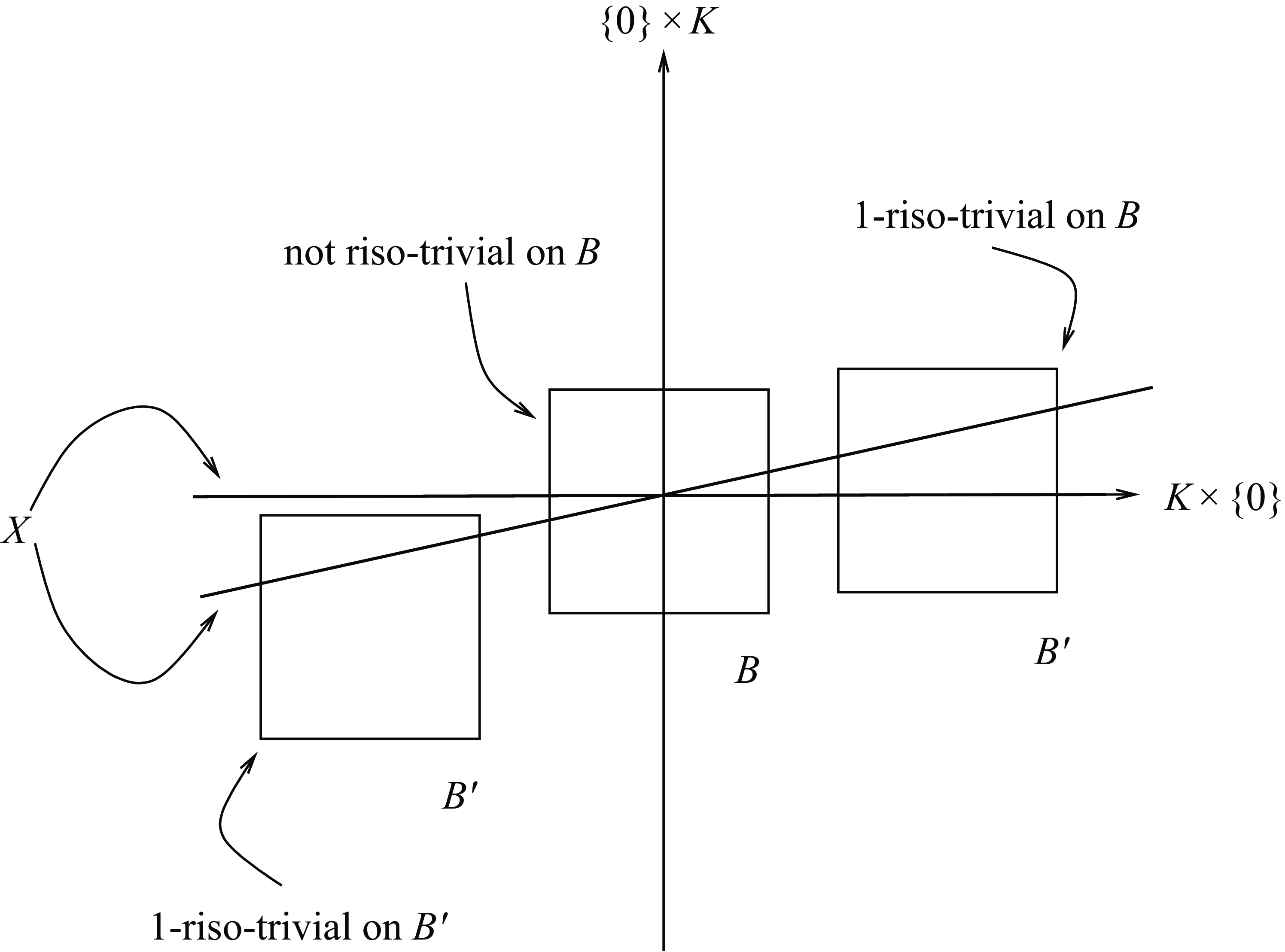
Example 3.13. Let
 $X \subset K^2$
be the union of the lines
 $K \times \{0\}$
and
 $\{(x,tx); x \in K\}$
(see Figure 2). Then
 $X$
is not riso-trivial on every ball
 $B$
containing the origin. If
 $B' \subset K^2$
is a ball not containing the origin, then
 $X$
is clearly
 $1$
-riso-trivial on
 $B'$
if
 $B'$
meets only one of the two lines, but even if
 $B'$
meets both lines,
 $X$
is
 $1$
-riso-trivial on
 $B'$
, since the two lines can be made parallel using a risometry. Overall, we obtain that Theorem 3.8 yields only the set
 $\{(0,0)\}$
.
4. Motivic integrals
In this section, we give a brief review of motivic integration, in order to fix notation and conventions (for all the details concerning this theory see [Reference Cluckers and LoeserCL08] or [Reference Cluckers and LoeserCL15]). In addition, we introduce the notion of limits of constructible motivic functions and prove some basic properties, adapting ideas from [Reference ForeyFor17, Section 3.1].
In [Reference Cluckers and LoeserCL15] motivic integration is introduced under axiomatic assumptions stated as [Reference Cluckers and LoeserCL15, Definition 3.9]. By [Reference Cluckers, Halupczok and Rideau-KikuchiCHR22, Theorem 5.8.2], those assumptions are satisfied for
 $\mathcal {L}$
and
 $K$
as in Definition 2.5.
Notation 4.1. For a valued field
 $K$
with residual field
 $k$
and value group
 $\mathbb {Z}$
as in § 1, let us first recall the definition given in [Reference Cluckers and LoeserCL08] of the ring of constructible motivic functions on some
 $\emptyset$
-definable set
 $X\subseteq K^n\times k^m\times \mathbb {Z}^r$
. For this purpose consider
 $\mathrm {RDef}_X$
the set of
 $\emptyset$
-definable subsets of
 $X\times k^p$
, for
 $p\in \mathbb {N}$
, equipped with their natural projection on
 $X$
. One denotes by
 $\mathcal {Q}_+(X)$
the Grothendieck semiring of
 $\emptyset$
-definable isomorphism classes
 $[Y]$
(more accurately classes of projections from
 $Y$
to
 $X$
),
 $Y\in \mathrm {RDef}_X$
, with the following relations for any
 $\emptyset$
-definable sets
 $Y,Z\in \mathrm {RDef}_X$
:
-
–
$[\emptyset ]=0$
; -
–
$[Y\cup Z]+[Y\cap Z]=[Y]+[Z]$
; -
–
$[Y\times Z]=[Y]\cdot [Z]$
.


We denote by the formal symbol
 $\mathbb {L}$
, the same symbol as used in Notation 2.2 to define the norm, the class
 $[X\times k]\in \mathcal {Q}_+(X)$
(actually the class of the projection of
 $X\times k$
on
 $X$
), and by
 $\mathcal {Q}(X)$
the associated abelian Grothendieck ring.
Still with the same symbol
 $\mathbb {L}$
we consider on the other hand the ring
 \begin{equation*} A:=\mathbb {Z}\left[\mathbb {L}, \mathbb {L}^{-1}, \left (\frac {1}{1-\mathbb {L}^i}\right )_{i\gt 0}\right], \end{equation*}
and
 $A_+$
its semigroup of nonnegative elements, where positivity is defined by evaluations
 $\mathbb {L}\mapsto r$
at
 $r$
, for any real number
 $r\gt 1$
. One defines the ring
 $\mathcal {P}(X)$
of Presburger functions, as a subring of the ring of functions
 $X\to A$
, as generated by constant functions,
 $\emptyset$
-definable functions
 $X\to \mathbb {Z}$
and functions
 $\mathbb {L}^\beta$
, with
 $\beta : X\to \mathbb {Z}$
 $\emptyset$
-definable. The semiring of functions of
 $\mathcal {P}(X)$
with nonnegative values (i.e. with values in
 $A_+$
) is denoted
 $\mathcal {P}_+(X)$
.
We denote by
 $\mathcal {P}_+^0(X)$
(respectively,
 $\mathcal {P}^0(X)$
) the sub-semiring (respectively, sub-ring) of
 $\mathcal {P}_+(X)$
(respectively,
 $\mathcal {P}$
(X)) generated by all characteristic functions
 $\mathbf {1}_Y$
, with
 $Y\subseteq X$
, and the constant function
 $\mathbb {L}-1$
. We can send
 $\mathcal {P}_+^0(X)$
(respectively,
 $\mathcal {P}(X)$
) in
 $\mathcal {Q}_+(X)$
(respectively,
 $\mathcal {Q}(X)$
) by
 $\mathbf {1}_Y \mapsto [Y]$
and
 $\mathbb {L}-1\mapsto \mathbb {L}-1$
, to form the semiring
 $\mathcal {C}_+(X)$
of nonnegative constructible motivic functions on
 $X$
as follows:
 \begin{equation*} \mathcal {C}_+(X):=\mathcal {Q}_+(X)\otimes _{\mathcal {P}_+^0(X)} \mathcal {P}_+(X). \end{equation*}
Likewise, we can sendthe ring
 $\mathcal {C}(X)$
of constructible motivic functions on
 $X$
as follows:
 \begin{equation*} \mathcal {C}(X):=\mathcal {Q}(X)\otimes _{\mathcal {P}^0(X)} \mathcal {P}(X). \end{equation*}
Remark 4.2. One can define (see [Reference Cluckers and LoeserCL08, Sections 4.2, 12.2]) a partial order on
 $\mathcal {P}(X)$
, denoted
 $\le$
, defined by
 \begin{equation*}\forall \varphi, \psi \in \mathcal {P}(X), \quad \varphi \le \psi \Longleftrightarrow \psi -\varphi \in \mathcal {P}_+(X).\end{equation*}
Similarly, one can define a partial preorder on
 $\mathcal {C}(X)$
, still denoted
 $\leq$
, by replacing
 $\mathcal {P}(X)$
by
 $\mathcal {C}(X)$
and
 $\mathcal {P}_+(X)$
by
 $\mathcal {C}_+(X)$
in the above definition. In both situations, when
 $\varphi \le \psi$
, one says that
 $\varphi$
is bounded by
 $\psi$
.
With this notation, in [Reference Cluckers and LoeserCL08, Theorem 10.1.1] the functor of motivic integration is defined as a functor from the category of
 $\emptyset$
-definable sets (equipped with their projection on
 $X$
) to the category of abelian semigroups, sending a
 $\emptyset$
-definable set
 $Y$
that projects on
 $X$
to the semigroup
 $\mathrm {I}_X\mathcal {C}_+(Y)\subseteq \mathcal {C}_+(Y)$
of nonnegative integrable functions on
 $Y$
over
 $X$
. To any
 $\emptyset$
-definable map
 $f:Y\to Z$
between
 $\emptyset$
-definable sets of
 $K^n\times k^m\times \mathbb {Z}^r$
it associates a morphism
 \begin{align*} f_!: \mathrm {I}_X \mathcal {C}_+(Y) \to \mathrm {I}_X \mathcal {C}_+(Z), \\[-12pt] \end{align*}
corresponding to integration in the fibres of
 $f$
twisted by a Jacobian, in the sense that for
 $f:Y\to Z$
and
 $g:Z \to W$
, and
 $\varphi \in \mathrm {I}_X\mathcal {C}_+(Y)$
,
 $(g\circ f)_!(\varphi )=g_!(f_!(\varphi ))$
.
Remark 4.3 [Reference Cluckers and LoeserCL08, Theorem 10.1.1 A0 (c)]. One has
 $\varphi \in \mathrm {I}_X\mathcal {C}_+(Y)$
if and only if
 $\varphi \in \mathrm {I}_Z\mathcal {C}_+(Y)$
and
 $f_{!}(\varphi )\in \mathrm {I}_X\mathcal {C}_+(Z)$
.
If
 $X=Z=\{pt\}$
, we have
 \begin{align*} \mathrm {I}_{X} \mathcal {C}_+(Z)=\mathrm {I}_{\{pt\}} \mathcal {C}_+(\{pt\})= \mathcal {C}_+(\{pt\})=\mathcal {Q}_+(\{pt\})\otimes _{\mathbb {N}[\mathbb {L}-1]} A_+, \\[-12pt] \end{align*}
where
 $\mathcal {Q}_+(\{pt\})$
is the Grothendieck semiring of
 $\emptyset$
-definable subsets of
 $k^m$
, for
 $m\in \mathbb {N}$
. In this situation,
 $f_!(\varphi )$
, denoted
 $\mu _n(\varphi )$
or
 $\mu (\varphi )$
when the context is clear, is the motivic integral of
 $\varphi$
on
 $Y$
,
 $\varphi$
is said integrable on
 $Y$
and we denote
 $\mathrm {I}\mathcal {C}_+(Y)$
instead of
 $\mathrm {I}_{\{pt\}}\mathcal {C}_+(Y)$
. Moreover, if
 $\varphi =\mathbf {1}_Y$
, then
 $\mu _n(\varphi )$
is simply denoted
 $\mu _n(Y)$
, or
 $\mu (Y)$
, and is called the motivic volume of
 $Y$
.
Remark 4.4. A normalization of the volume is made in order to obtain uniqueness of the functor of motivic integration, leading in particular to
 $\mu _1(\mathcal {O}_K)=1$
and
 $\mu _1(\mathcal {M}_K)=\mathbb {L}^{-1}$
(see [Reference Cluckers and LoeserCL08, Theorem 10.1.1, A7]).
We mention without going into detail that one can build motivic measures in all dimensions; that is to say, measures
 $\mu _d$
adapted to functions with support a
 $\emptyset$
-definable set of
 $K^n$
of dimension
 $d$
, with
 $d\in \mathbb {N}$
(see [Reference Cluckers and LoeserCL08, Section 6], [Reference Cluckers and LoeserCL15, Section 11]).
Remark 4.5. Let
 $X,Y$
be
 $\emptyset$
-definable subsets of
 $K^n\times k^m \times \mathbb {Z}^r$
, of dimension
 $d$
, say, such that
 $X\subset Y$
. Then, according to Remark 4.2,
 $\mathbf {1}_X$
is bounded by
 $\mathbf {1}_Y$
in
 $\mathcal {P}_+(Y)$
(or in
 $\mathcal {C}_+(Y)$
), since
 $\mathbf {1}_Y-\mathbf {1}_X=\mathbf {1}_{Y\setminus X}\in \mathcal {P}_+(Y)$
, and thus integrating, by linearity of the integral and preservation of nonnegativity, one gets
 $\mu _d(X)\le \mu _d(Y)$
.
In what follows we mainly consider the family version of this construction (see [Reference Cluckers and LoeserCL08, Section 14], or [Reference Cluckers and LoeserCL15] for a specific construction of integration in fibres in the more general context of residue fields of all characteristics), i.e. for some integers
 $r,s,t$
, we consider
 $\Lambda \subset K^r\times k^s\times \mathbb {Z}^t$
, a
 $\emptyset$
-definable set, and
 $\emptyset$
-definable families
 $Y=(Y_\lambda )_{\lambda \in \Lambda }$
,
 $Z=(Z_\lambda )_{\lambda \in \Lambda }$
compatible with the projection on
 $X$
, in the sense that
 $Y$
and
 $Z$
are given by maps
 $Y\to X\to \Lambda$
and
 $Z\to X\to \Lambda$
.
Notation 4.6. For
 $n,m,r\in \mathbb {N}$
,
 $Y,Z\subseteq K^n\times k^m\times \mathbb {Z}^r$
 $\emptyset$
-definable sets,
 $f:Y\to Z$
a
 $\emptyset$
-definable map and
 $\varphi \in \mathcal {C}(Z)$
we denote by
 $f^*(\varphi )\in \mathcal {C}(Y)$
the pull-back of
 $\varphi$
along
 $f$
, which should be understood as the composition
 $\varphi \circ f$
. For
 $f$
, given by a commutative diagram

for
 $\lambda \in \Lambda$
, we denote by
 $f_{\lambda }:Y_\lambda \to Z_\lambda$
the restriction of
 $f$
to the fibres of
 $Y$
and
 $Z$
above
 $\lambda$
. We also denote, with a slight abuse of notation, by
 $i_\lambda$
the inclusion of
 $Y_\lambda$
(respectively, of
 $Z_\lambda$
) in
 $Y$
(respectively, in
 $Z$
).
One can then define [Reference Cluckers and LoeserCL08, Theorem 14.1.1] a morphism
 \begin{equation*} f_{!\Lambda }: \mathrm {I}_X \mathcal {C}_+(Y\to \Lambda ) \to \mathrm {I}_X \mathcal {C}_+(Z\to \Lambda ), \end{equation*}
that associates to any
 $\varphi$
in the semigroup
 $\mathrm {I}_X \mathcal {C}_+(Y\to \Lambda )$
of integrable nonnegative constructible motivic functions, graded with respect to relative dimension (relative to the map
 $Y\to X$
), the element
 $f_{!\Lambda }(\varphi )$
of
 $\mathrm {I}_X \mathcal {C}_+(Z\to \Lambda )$
.
Remark 4.7. By [Reference Cluckers and LoeserCL08, Proposition 14.2.1] one has for any
 $\lambda \in \Lambda$
,
 \begin{equation*}i^*_\lambda (f_{!\Lambda }(\varphi ))=f_{\lambda !}(i^*_\lambda (\varphi )).\end{equation*}
This is why we will often denote
 $f_{!\Lambda }(\varphi )$
by
 $(f_{\lambda !}(\varphi _\lambda ))_{\lambda \in \Lambda }$
; that is to say, we will consider the constructible motivic function
 $f_{!\Lambda }(\varphi )$
as a family of measures over
 $\Lambda$
.
In the particular case
 $f:Y\to \Lambda$
, i.e,
 $Z=X=\Lambda$
and the map
 $f$
is the map defining the family
 $Y$
, we have
 $f_\lambda : Y_\lambda \to \{\lambda \}$
, and consequently
 $f_{!\Lambda }(\varphi )=(\mu (\varphi _\lambda ))_{\lambda \in \Lambda }\in \mathcal {C}_+(\Lambda )$
. In this situation
 $f_{!\Lambda }(\varphi )$
is the integration of
 $\varphi$
in the fibres of
 $Y\to \Lambda$
, and we denote
 $f_{!\Lambda }$
by
 $\mu _\Lambda$
, or in a more intuitive way by
 $\left(\vphantom{{}^{1}_{1}} \smash{\int _{y\in Y_\lambda }} \varphi _\lambda (y) \ {\rm d}y\right)_{\lambda \in \Lambda }$
. Furthermore, when
 $\varphi =\mathbf {1}_Y$
, we have
 $\mu _\Lambda (\varphi )=(\mu (Y_\lambda ))_{\lambda \in \Lambda }$
.
Remark 4.8. In the situation where
 $\pi : X\times Y\to X$
is the standard projection, then
 $\pi _!=\pi _{!X}$
, and thus
 $\pi _!(\varphi )\in \mathrm {I}_X\mathcal {C}_+(X)=\mathcal {C}_+(X)$
is the family
 $\left (\mu (\varphi _x)\right )_{x\in X}=\left (\int _{Y} \varphi (x,y) \ {\rm d}y\right )_{x\in X}$
of motivic integrals of
 $\varphi$
in the fibres
 $\{x\}\times Y$
, for
 $x\in X$
(see [Rai20, Remarque 5.3.4.6.1]).
We now introduce a notion of convergence of nonnegative constructible motivic functions and measures. A variant of this has already been considered in [Reference ForeyFor17, Section 3.1], with the difference here being that we do not take mean values in the notion of convergence.
One can uniquely extend the degree (in
 $\mathbb {L}$
) on
 $\mathbb {Z}[\mathbb {L}]$
to a degree
 $\deg$
on
 $A_+$
(respectively, on
 $A$
). We then define a topology on
 $A_+$
such that the convergence to
 $0$
of a sequence
 $(a_n)_{n\in \mathbb {N}}$
with elements in
 $A_+$
is the convergence to
 $-\infty$
of the sequence
 $(\deg (a_n))_{n\in \mathbb {N}}$
. This yields a notion of convergence of functions in
 $\mathcal {P}_+(\mathbb {N})$
, and also in a variant with additional parameters.
Definition 4.9. Let
 $X,Y\subset K^n\times k^m\times \mathbb {Z}^r$
be
 $\emptyset$
-definable, and let
 $\psi \in \mathcal {P}_+(X \times Y)$
and
 $\psi ' \in \mathcal {P}_+(X)$
be nonnegative Presburger functions.
-
(1) If
$Y = \mathbb {N}$
, we say that
$\psi (\cdot,r)$
converges to
$\psi '$
, for
$r \to +\infty$
, if, for each
$x \in X$
, we have
$\lim _{r \to +\infty }\psi (x,r) = \psi '(x)$
, in the sense of convergence in
$A_+$
described above. -
(2) If
$Y = \mathbb {N}$
, we say that
$\psi (\cdot,r)$
is increasing for
$r \to +\infty$
if, for each
$(x,r)\in X \times \mathbb {N}$
, we have
$\psi (x,r+1) - \psi (x,r) \in A_+$
. -
(3) We say that
$\psi (x, y)$
is bounded by
$\psi '$
(uniformly in
$y$
) if, for each
$(x,y)\in X \times Y$
, we have
$\psi '(x) - \psi (x,y) \in A_+$
(see also Remark 4.2).


We now extend these notions to constructible motivic functions. By orthogonality of the residue field and the value group, any function
 $\psi \in \mathcal {C}_+(X \times \mathbb {N})$
may be written as a finite sum
 \begin{equation} \psi =\sum _{i=1}^\ell c_i\otimes \psi _i, \end{equation}
where
 $c_i\in \mathcal {Q}_+(X)$
and
 $\psi _i\in \mathcal {P}_+(X \times \mathbb {N})$
(see [Reference Cluckers and LoeserCL08, Section 5.3] or [Reference Cluckers and LoeserCL15, Proposition 7.5] for details).
Definition 4.10. Let
 $X\subset K^n\times k^m\times \mathbb {Z}^r$
be
 $\emptyset$
-definable and let
 $\psi \in \mathcal {C}_+(X \times \mathbb {N})$
and
 $\psi ' \in \mathcal {C}_+(X)$
be nonnegative constructible motivic functions. We say that
 $\psi (\cdot,r)$
converges to
 $\psi '$
(respectively, is increasing, is bounded by
 $\psi '$
) if there exist
 $c_i$
and
 $\psi _i$
as in (9) and
 $\psi '_i \in \mathcal {P_+}(X)$
such that
 $\psi ' = \sum _i c_i\otimes \psi '_i$
and such that for each
 $i$
,
 $\psi _i$
converges to
 $\psi '_i$
(respectively, is increasing, is bounded by
 $\psi '_i$
). For the notion of boundedness, we also allow arbitrary definable sets
 $Y\in K^n\times k^m \times \mathbb {Z}^r$
instead of
 $\mathbb {N}$
.
Remark 4.11. The notions of boundedness and increasingness can equivalently be defined directly using
 $\mathcal {C}_+$
, that is, without passing through
 $\mathcal {P}_+$
(see also Remark 4.2):
 $\psi \in \mathcal {C}_+(X \times Y)$
is bounded by
 $\psi ' \in \mathcal {C}_+(X)$
if there exists
 $\phi \in \mathcal {C}_+(X \times Y)$
such that
 $\psi + \phi = \psi '$
, and
 $\psi \in \mathcal {C}_+(X \times \mathbb {N})$
is increasing if there exists
 $\phi \in \mathcal {C}_+(X \times \mathbb {N})$
such that
 $\psi + \phi = \psi '$
, where
 $\psi '(x,r) = \psi (x,r+1)$
.
Notation 4.12. For
 $n,m,r\in \mathbb {N}$
,
 $X\subseteq K^n\times k^m\times \mathbb {Z}^r$
an
 $\emptyset$
-definable set and
 $\phi,\psi \in \mathcal {C}_+(X)$
, we write
 $\phi \le \psi$
if
 $\phi$
is bounded by
 $\psi$
in the sense of Definition 4.10.
Remark 4.13. The limit
 $\psi '$
, if it exists, is well defined; that is, it does not depend on the choice of the representation of
 $\psi$
in the form (9). To see this, denote by
 $\mathcal {P}^{\mathrm {lim}}_+(X \times \mathbb {N}) \subset \mathcal {P}_+(X \times \mathbb {N})$
and
 $\mathcal {C}^{\mathrm {lim}}_+(X \times \mathbb {N}) \subset \mathcal {C}_+(X \times \mathbb {N})$
the sub-semirings of converging nonnegative Presburger and constructible motivic functions, where the convergence is defined in Definition 4.10. By definition of
 $\mathcal {C}^{\mathrm {lim}}_+(X \times \mathbb {N})$
, we have
 \begin{equation*}\mathcal {C}^{\mathrm {lim}}_+(X \times \mathbb {N})= \mathcal {Q}_+(X)\otimes _{\mathcal {P}_+^0(X)} \mathcal {P}^{\mathrm {lim}}_+(X \times \mathbb {N}),\end{equation*}
where we use again the same isomorphism as in (9), provided by [Reference Cluckers and LoeserCL08, Section 5.3] or [Reference Cluckers and LoeserCL15, Proposition 7.5], to omit the
 $\mathbb {N}$
from the left-hand side of the tensor product and from the
 $\mathcal {P}_+^0$
.
The map
 $h\colon \mathcal {P}^{\mathrm {lim}}_+(X \times \mathbb {N}) \to \mathcal {P}_+(X)$
sending a function to its limit induces the identity on
 $\mathcal {P}_+^0(X)$
, so we can apply the functor
 $S \mapsto \mathcal {Q}_+(X)\otimes _{\mathcal {P}_+^0(X)} S$
to that map
 $h$
to define the limit on
 $\mathcal {C}^{\mathrm {lim}}_+(X \times \mathbb {N})$
in a way which is independent of how we write a function
 $\psi \in \mathcal {C}^{\mathrm {lim}}_+(X \times \mathbb {N})$
as in (9).
The following lemma and remarks give the properties of this notion of convergence that we need. The proof of the lemma requires a detailed understanding of the tensor product
 $\mathcal {Q}_+(X) \otimes _{\mathcal {P}^0_+(X)} \mathcal {P}_+(X \times \mathbb {N})$
. We give those details in Appendix A; more precisely, we use Lemma A.4 from the appendix in the proof of the following lemma.
Lemma 4.14.
Suppose that we have
 $\psi _1, \psi _2\in \mathcal {C}_+(X \times \mathbb {N})$
such that
 $\psi _1(\cdot, r) + \psi _2(\cdot, r)$
tends to
 $0 \in \mathcal {C}_+(X)$
(for
 $r \to +\infty$
). Then
 $\psi _1(\cdot, r)$
and
 $\psi _2(\cdot, r)$
also tend to
 $0$
for
 $r \to +\infty$
.
Note that this lemma would most likely be false if, instead of working with
 $\mathcal {C}_+(X \times \mathbb {N})$
and
 $\mathcal {C}_+(X)$
, we worked with the image of these semirings in the rings
 $\mathcal {C}(X \times \mathbb {N})$
and in
 $\mathcal {C}(X)$
, respectively. Indeed, it seems plausible that for sufficiently bad residue fields, one can find some
 $\phi \in \mathcal {C}(X) \setminus \{0\}$
satisfying
 $2\phi = 0$
and which lies in the image of
 $\mathcal {C}_+(X)$
. In other words, we would not even have that
 $\psi _1+\psi _2 = 0$
implies
 $\psi _1 = \psi _2 = 0$
.
Proof of Lemma 4.14.
We first collect some facts that will serve as prerequisites to apply Lemma A.4. All those facts follow directly from the definitions of the corresponding semirings. Given
 $\psi \in P_+(X \times \mathbb {N})$
, we write
 $\psi \to 0$
to say that
 $\psi (\cdot, r)$
converges to
 $0$
when
 $r$
goes to
 $+\infty$
(in the sense of Definition 4.10).
-
(1) For every
$\emptyset$
-definable set
$Y$
and every
$\phi, \phi ' \in \mathcal {Q}_+(Y)$
, we have the following two implications:-
(a)
$\phi +\phi ' = 0$
implies
$\phi = \phi ' = 0$
; -
(b)
$\phi \cdot \phi ' = 0$
implies
$\phi = 0$
or
$\phi ' = 0$
.
-
-
(2) For every
$\emptyset$
-definable set
$Y$
and every
$\phi, \phi ' \in \mathcal {P}_+(Y)$
, we have the following two implications:-
(a)
$\phi +\phi ' = 0$
implies
$\phi = \phi ' = 0$
; -
(b)
$\phi \cdot \phi ' = 0$
implies
$\phi = 0$
or
$\phi ' = 0$
.
-
-
(3) For every
$\phi _1,\phi _2 \in \mathcal {P}_+(X \times \mathbb {N})$
and every
$\phi _0 \in \mathcal {P}_+^0(X)$
, we have the following two implications:-
(a)
$\phi _1 + \phi _2 \to 0$
implies
$\phi _1 \to 0$
and
$\phi _2 \to 0$
; -
(b)
$\phi _0 \cdot \phi _1 \to 0$
implies
$\phi _1 \to 0.$
-


Suppose now that
 $\psi _1, \psi _2$
are given as in the lemma. Write both of them as sums as in (9):
 \begin{equation} \psi _1 =\sum _{i=1}^{\ell _1} c_{1,i}\otimes \psi _{1,i}, \quad \psi _2 =\sum _{i=1}^{\ell _2} c_{2,i}\otimes \psi _{2,i}, \end{equation}
for some
 $c_{j,i} \in \mathcal {Q}_+(X)$
and
 $\psi _{j,i}\in \mathcal {P}_+(X \times \mathbb {N})$
. By assumption,
 $\psi _3 := \psi _1 + \psi _2$
converges to
 $0$
, i.e. it can also be written as such a sum
 \begin{equation} \psi _3 =\sum _{i=1}^{\ell _3} c_{3,i}\otimes \psi _{3,i}, \end{equation}
where each
 $\psi _{3,i}$
converges, say to some
 $\phi _{3,i} \in \mathcal {P}_+(X)$
, and such that the sum
 \begin{equation} \sum _{i=1}^{\ell _3} c_{3,i}\otimes \phi _{3,i} \end{equation}
is equal to
 $0$
in
 $\mathcal {C}_+(X) = \mathcal {Q}_+(X) \otimes _{\mathcal {P}_+^0(X)} \mathcal {P}_+(X)$
. We may without loss of generality assume
 $c_{3,i} \ne 0$
for each
 $i$
.
Apply Lemma A.4 to
 $S := \mathcal {P}_+^0(X)$
,
 $U_1 := \{0\} \subset \mathcal {Q}_+(X)$
and
 $U_2 := \{0\} \subset \mathcal {P}_+(X)$
. Note that the assumptions of Lemma A.4 concerning
 $S$
,
 $U_1$
and
 $U_2$
are satisfied by (2), (1) and (2), respectively. Since the sum (12) lies in the sub-semimodule
 $U \subset \mathcal {Q}_+(X) \otimes _{\mathcal {P}^0_+(X)} \mathcal {P}_+(X)$
defined in Lemma A.4, we obtain
 $\phi _{3,i} = 0$
for each
 $i$
(since we assumed
 $c_{3,i} \ne 0$
). In other words, for each
 $i$
, we have
 $\psi _{3,i} \to 0$
.
Now apply Lemma A.4 once more, this time to
 $S := \mathcal {P}_+^0(X)$
,
 $U_1 := \{0\} \subset \mathcal {Q}_+(X)$
and
 $U_2 := \{\phi \in \mathcal {P}_+(X \times \mathbb {N}); \phi \to 0\}$
. The assumptions of Lemma A.4 concerning
 $S$
,
 $U_1$
and
 $U_2$
are satisfied by (2), (1) and (3), respectively. Since in (11),
 $\psi _{3,i} \to 0$
for each
 $i$
,
 $\psi _3$
lies in the sub-semimodule
 $U \subset \mathcal {Q}_+(X) \otimes _{\mathcal {P}^0_+(X)} \mathcal {P}_+(X \times \mathbb {N})$
defined in Lemma A.4, so the lemma implies that
 $\psi _1$
and
 $\psi _2$
lie in
 $U$
. By definition of
 $U$
, elements of
 $U$
converge to
 $0$
, so we are done.
Remark 4.15 (Monotone convergence). A
 $\emptyset$
-definable subset
 $X$
of
 $K^n\times \mathbb {N}$
with projection
 $\pi : X \mapsto \mathbb {N}$
, and fibres
 $\pi ^{-1}(p)=X_p$
, such that
 $(X_p)_{p\in \mathbb {N}}$
is uniformly bounded with respect to
 $p\in \mathbb {N}$
, and which is an increasing sequence with respect to the inclusion relation, gives rise to the bounded increasing function
 $\varphi =\pi _{!\mathbb {N}}(\mathbf {1}_{X})=(\mu (X_p))_{p\in \mathbb {N}}\in \mathcal {C}_+(\mathbb {N})$
. It follows that this function converges as
 $p$
goes to
 $+\infty$
, and by definition of the motivic integral, that its limit is
 $\mu \left ( \bigcup _{i=0}^{+\infty } X_i\right )$
(see [Reference ForeyFor17, Lemma 5.1] for more details).
Remark 4.16. Let
 $X \subset K^n$
be a bounded
 $\emptyset$
-definable set of dimension
 $d$
and, for
 $r \in \mathbb {Z}$
, let
 $T_r(X)=\{x\in K^n;\exists y\in X, \mathrm {val}(y-x)\ge r\}$
be the corresponding tubular neighbourhood. Then, for
 $r \ge 0$
,
 $\mu _n(T_r(X))$
is bounded by
 $(\mathbb {L}^{-r})^{n-d}\cdot C$
for some constant
 $C \in \mathcal {C}_+(\{pt\})$
depending only on
 $X$
(i.e.
 $(\mathbb {L}^{-r})^{n-d}\cdot C - \mu _n(T_r(X)) \in \mathcal {C}_+(\mathbb {N})$
). Indeed, by cell decomposition with
 $1$
-Lipschitz centres,
 $X$
can be partitioned into a finite
 $\emptyset$
-definable family of sets
 $X_\xi$
each of which is, up to a permutation of coordinates, the graph of a
 $1$
-Lipschitz function
 $f_\xi$
on a subset
 $\bar X_\xi$
of
 $K^d$
(for more details about this kind of cell decomposition, see Step 1 of the proof of Theorem 7.1). This implies that
 $\mu _n(T_r(X_\xi ))$
is bounded by
 $\mu _d(T_0(\bar X_\xi ))\cdot (\mathbb {L}^{-r})^{n-d}$
. Finally note that, applying Remark 4.5, the volume of the tubular neighbourhood of
 $X$
is bounded by the sum of the volume of the tubular neighbourhoods of the
 $X_\xi$
.
5. A partial preorder for constructible motivic functions
In this section we define and study a partial preorder
 $\preccurlyeq$
on the set of integrable constructible motivic functions. We show that
 $\preccurlyeq$
has the required properties with respect to our proof strategy for the nonarchimedean version of inequality (5) relating the motivic Vitushkin invariants and the motivic metric entropy. In particular,
 $\preccurlyeq$
is compatible with integration (Lemma 5.10). We start by defining the set
 $\mathrm {I}\mathcal {C}_{\succcurlyeq 0}(X)$
of constructible motivic functions that are nonnegative with respect to our new relation, and observe that nonnegative constructible motivic functions in the sense of § 3 (that is to say, when nonnegativity is defined through the ring
 $A_+$
) are also nonnegative regarding our definition of
 $\preccurlyeq$
. Note that with respect to our preorder
 $\preccurlyeq$
there are strictly more nonnegative functions than with respect to the preorder
 $\le$
defined by
 $\mathrm {I}\mathcal {C}_{+}(X)$
(see Example 5.4).
Definition 5.1. Let
 $m,n,r\in \mathbb {N}$
and
 $X\subseteq K^n\times k^m\times \mathbb {Z}^r$
be a
 $\emptyset$
-definable set. We denote by
 $\mathrm {I}\mathcal {C}_{\succcurlyeq 0}(X)$
the subset of
 $\mathrm {I}\mathcal {C}(X)$
consisting of the constructible motivic functions
 $F\in \mathrm {I}\mathcal {C}(X)$
for which there exist
 $\emptyset$
-definable sets
 $Y, Z \subseteq k^{m'}$
for some
 $m'\in \mathbb {N}$
, a
 $\emptyset$
-definable surjection
 $f\colon Z \twoheadrightarrow Y$
with finite fibres and a constructible motivic function
 $\varphi \in \mathrm {I}\mathcal {C}_+(Y \times X)$
such that the following equality holds in
 $\mathrm {I}\mathcal {C}(X)$
:
 \begin{equation} F = \pi _{X!}f_X^*\varphi - \pi _{X!}\varphi, \end{equation}
where
 $f_X: Z \times X \twoheadrightarrow Y \times X, (z,x) \mapsto (f(z), x)$
, and
 $\pi _X$
is the standard projection onto
 $X$
.

Remark 5.2. Note that in (13),
 $\varphi$
and
 $f^*_X\varphi$
are indeed integrable along
 $\pi _X$
:. For
 $\varphi$
, this follows from the assumption
 $\varphi \in \mathrm {I}\mathcal {C}_+(Y \times X)$
(which implies
 $\varphi \in \mathrm {I}_{X}\mathcal {C}_+(Y \times X)$
by Remark 4.3. For
 $f^*_X\varphi$
, note that since
 $f$
has finite fibres,
 $\varphi \in \mathrm {I}_X\mathcal {C}_+(Y \times X)$
implies
 $f^*_X\varphi \in \mathrm {I}_X\mathcal {C}_+(Z \times X)$
.
In view of Remark 4.8, we have a more intuitive expression for
 $F\in \mathrm {I}\mathcal {C}_{\succcurlyeq 0}(X)$
:
 \begin{equation*} F(x)=\mu _X(f_X^*\varphi _x)-\mu _X(\varphi _x)= \int _{Z} \varphi \circ f_X(z,x) \ {\rm d}z - \int _{Y} \varphi (y,x) \ {\rm d}y. \end{equation*}
One could imagine various variants of Definition 5.1; we will see in Lemma 5.11 and Remark 5.12 below that some variants lead to an equivalent definition.
Lemma 5.3.
For
 $m,n,r\in \mathbb {N}$
and
 $X\subseteq K^n\times k^m\times \mathbb {Z}^r$
a
 $\emptyset$
-definable set, one has that the image of
 $\mathrm {I}\mathcal {C}_+(X)$
in
 $\mathrm {I}\mathcal {C}(X)$
is contained in
 $\mathrm {I}\mathcal {C}_{\succcurlyeq 0}(X)$
.
Proof.
Let
 $F \in \mathrm {I}\mathcal {C}_+(X)$
be given. Set
 $Y := \{0\}\subseteq k$
,
 $Z = \{0, 1\}\subseteq k$
,
 $f(0) = f(1) = 0$
and
 $\varphi (0,\cdot ) = F$
. Then
 $\pi _{X!}(f_X^*\varphi ) - \pi _{X!}(\varphi ) = 2F - F = F$
.
Example 5.4. If
 $k=\mathbb {C}$
, for instance, one can give an example of a constructible motivic function in
 $\mathrm {I}\mathcal {C}_{\succcurlyeq 0}(X)$
but not in the image of
 $\mathrm {I}\mathcal {C}_+(X)$
in
 $\mathrm {I}\mathcal {C}(X)$
. Indeed, let us consider the constructible motivic function
 $\varphi =[Z]-1$
for
 $Z = \{\pm \sqrt 2\} \subset \mathbb {C}$
. In view of Lemma 5.11, since there is a
 $\emptyset$
-definable surjection from the
 $\emptyset$
-definable set
 $Z$
to the point, we have
 $\varphi \in \mathrm {I}\mathcal {C}_{\succcurlyeq 0}(X)$
.
Let us now show that
 $\varphi$
does not lie in the image of
 $\mathrm {I}\mathcal {C}_+(X)$
. This amounts to showing that there is no
 $\emptyset$
-definable set
 $Y \subset \mathbb {C}^m$
(for some
 $m$
) and injective
 $\emptyset$
-definable map
 $f\colon \{pt\} \sqcup Y \to Z \sqcup Y$
. Suppose the existence of
 $Y$
and
 $f$
. Without loss of generality, they are defined by quantifier-free formulas, so that we also obtain a
 $\emptyset$
-definable injection between the restrictions of those sets to any subfield
 $F \subset \mathbb {C}$
. We pick
 $F$
to be a pseudo-finite field not containing the square roots of
 $2$
. Then
 $f$
further induces a bijection in some sufficiently big finite field not containing the square roots of
 $2$
. However, this is not possible for cardinality reasons.
We typically need this kind of comparison allowed by our preorder in equation (24) of the proof of Theorem 8.6.
Note that if the residue field has definable Skolem functions, the inclusion of Lemma 5.3 is an equality, as shown by the following lemma.
Lemma 5.5.
If the residue field
 $k$
of
 $K$
has definable Skolem functions, then for any
 $m,n,p,r\in \mathbb {N}$
and any
 $\emptyset$
-definable set
 $X\subseteq K^n\times k^m\times \mathbb {Z}^r$
, we have
 $\mathrm {I}\mathcal {C}_{\succcurlyeq 0}(X) = \mathrm {I}\mathcal {C}_+(X)$
.
Proof.
The inclusion
 $ \mathrm {I}\mathcal {C}_+(X) \subseteq \mathrm {I}\mathcal {C}_{\succcurlyeq 0}(X)$
is Lemma 5.3. Now let
 $F \in \mathrm {I}\mathcal {C}_{\succcurlyeq 0}(X)$
be given, witnessed by
 $Z \overset {f}{\twoheadrightarrow } Y$
, with
 $Y,Z\subset k^{m'}$
for
 $m'\in \mathbb {N}$
, and
 $\varphi \in \mathrm {I}\mathcal {C}_+(Y \times X)$
. That is to say,
 $F = \pi _{X!}(f_{X}^*\varphi ) - \pi _{X!}(\varphi )$
.
By the assumption that the residue field has definable Skolem functions (and using that the value group
 $\mathbb {Z}$
also has definable Skolem functions) we find a
 $\emptyset$
-definable map
 $g\colon Y \to Z$
such that
 $f\circ g$
is the identity on
 $Y$
. Set
 $Z' := Z \setminus g(Y)$
, and let
 $f'\colon Z' \to Y$
be the restriction of
 $f$
to
 $Z'$
. Then
 $F = \pi _{X!}(f'^{*}_{X}\varphi )$
, and
 $\pi _{X!}(f'^{*}_{X}\varphi )$
lies in
 $\mathrm {I}\mathcal {C}_+(X)$
, since
 $\varphi$
lies in
 $\mathrm {I}\mathcal {C}_+(Y \times X)$
(using Remark 4.3 in particular).
Lemma 5.6.
For
 $m,n,r\in \mathbb {N}$
and
 $X\subseteq K^n\times k^m\times \mathbb {Z}^r$
a
 $\emptyset$
-definable set, let
 $F_1, F_2\in \mathrm {I}\mathcal {C}_{\succcurlyeq 0}(X)$
. Then
 $F_1+F_2\in \mathrm {I}\mathcal {C}_{\succcurlyeq 0}(X)$
.
In particular, we obtain a partial preorder on
 $\mathcal {C}(X)$
by setting
 \begin{equation*}F \preccurlyeq G \Longleftrightarrow G - F \in \mathrm {I}\mathcal {C}_{\succcurlyeq 0}(X).\end{equation*}
Proof.
Suppose that
 $F_1, F_2 \in \mathrm {I}\mathcal {C}_{\succcurlyeq 0}(X)$
are witnessed by
 and
 $\varphi _i \in \mathrm {I}\mathcal {C}_+(Y_i \times X)$
, that is to say,
 $F_i = \pi _{X!}(f_{iX}^*\varphi _i) - \pi _{X!}(\varphi _i)$
. Without loss of generality, we can assume that
 $Y_1$
and
 $Y_2$
are disjoint subsets in
 $k^m$
, for some
 $m\in \mathbb {N}$
and similarly for
 $Z_1$
and
 $Z_2$
. Set
 $Y = Y_1 \sqcup Y_2$
,
 $Z = Z_1 \sqcup Z_2$
, define
 $f\colon Z \to Y$
such that
 $f_{\restriction Z_i} = f_i$
and
 $\varphi \in \mathrm {I}\mathcal {C}_+(Y \times X)$
such that
 $\varphi _{\restriction Y_i \times X} = \varphi _i$
. Then
 $F_1 + F_2 = \pi _{X!}(f_X^*\varphi ) - \pi _{X!}(\varphi )$
.
Remark 5.7. For
 $m,n,r\in \mathbb {N}$
and
 $X\subseteq K^n\times k^m\times \mathbb {Z}^r$
a
 $\emptyset$
-definable set, when
 $F\in \mathrm {I}\mathcal {C}_{\succcurlyeq 0}(X)$
and
 $G\in \mathcal {C}_+(X)$
, then
 $F \cdot G\in \mathrm {I}\mathcal {C}_{\succcurlyeq 0}(X)$
, since in Definition 5.1, we can replace
 $\varphi$
by
 $\varphi \cdot G$
.
Question 5.8. However, we do not know whether
 $F, G\in \mathrm {I}\mathcal {C}_{\succcurlyeq 0}(X)$
implies
 $F\cdot G\in \mathrm {I}\mathcal {C}_{\succcurlyeq 0}(X)$
.
The partial preorder on
 $\mathrm {I}\mathcal {C}(X)$
is compatible with pull-back.
Lemma 5.9.
For
 $m,n,r\in \mathbb {N}$
and
 $\emptyset$
-definable sets
 $X, \tilde {X}\subseteq K^n\times k^m\times \mathbb {Z}^r$
, if
 $g\colon \tilde X \to X$
,
 $1_{\tilde {X}}$
is in
 $\mathrm {I}_X\mathcal {C}_+(\tilde {X}\overset {g}{\to } X)$
and
 $F \in \mathrm {I}\mathcal {C}_{\succcurlyeq 0}(X)$
, then
 $g^*F \in \mathrm {I}\mathcal {C}_{\succcurlyeq 0}(\tilde X)$
.
Proof.
Let
 $F \in \mathrm {I}\mathcal {C}_{\succcurlyeq 0}(X)$
be witnessed by
 , and
 $\varphi \in \mathrm {I}\mathcal {C}_+(Y \times X)$
. That is to say,
 $F = \pi _{X!}(f_{X}^*\varphi ) - \pi _{X!}(\varphi )$
. Set
 $\tilde \varphi := g_Y^*\varphi$
, where
 $g_Y\colon Y \times \tilde X \to Y \times X, (y,\tilde x) \mapsto (y, g(\tilde x))$
. Then
 $\tilde \varphi \in \mathrm {I}\mathcal {C}(Y \times \tilde X)$
, and
 $g^* F \in \mathrm {I}\mathcal {C}_{\succcurlyeq 0}(X)$
is witnessed by
 and
 $\tilde \varphi$
(see [Reference Cluckers and LoeserCL08, Theorem 10.1.1 A3] for
 $\tilde \varphi \in \mathrm {I}\mathcal {C}_+(Y\times \tilde {X})$
).
The partial order is compatible with integration, in the following sense.
Lemma 5.10.
Let
 $m,n,r\in \mathbb {N}$
,
 $U,V\subseteq K^n\times k^m\times \mathbb {Z}^r$
be
 $\emptyset$
-definable sets,
 $F_1,F_2\in \mathrm {I}_V\mathcal {C}(U\times V)$
, and
 $\pi _V: U\times V\to V$
the standard projection. If
 $F_1 \preccurlyeq F_2$
, then
 $\pi _{V!}F_1 \preccurlyeq \pi _{V!}F_2$
. This may be written, using the integral notation, as
 \begin{equation*} \int _U F_1(u,\cdot ) \ {\rm d}u \preccurlyeq \int _U F_2(u,\cdot ) \ {\rm d}u. \end{equation*}
Proof.
By additivity of the integral, it suffices to prove that for
 $F \in \mathrm {I}\mathcal {C}_{\succcurlyeq 0}(U \times V)$
, we have
 $\tilde F := \pi _{V!}F \in \mathrm {I}\mathcal {C}_{\succcurlyeq 0}(V)$
.
Let 
 $\varphi \in \mathrm {I} \mathcal {C}_+(Y \times U\times V)$
witness that
 $F \succcurlyeq 0$
. That is to say,
 $F = \pi _{U \times V!}(f_{U \times V}^*\varphi ) - \pi _{U \times V !}(\varphi )$
.
By Remark 4.3,
 $\varphi \in \mathrm {I}_{Y\times V}\mathcal {C}_+(Y\times U\times V)$
. We can therefore define
 $ \tilde \varphi := \pi _{Y \times V!}\varphi$
, and again by Remark 4.3 we have
 $\tilde \varphi \in \mathrm {I}\mathcal {C}_+(Y \times V)$
.
Then  and
 $\tilde \varphi$
witness
 $\tilde F \ge 0$
. Indeed, we have
 \begin{align*} \tilde F &= \pi _{V!}\pi _{U\times V!}f_{U \times V}^*\varphi - \pi _{V!}\pi _{U\times V!}\varphi \\ &= \pi _{V!}\pi _{Z \times V!}f_{U \times V}^*\varphi - \pi _{V!}\pi _{Y \times V!} \varphi \\ &= \pi _{V!}f_{V}^*\pi _{Y \times V!}\varphi - \pi _{V!}\pi _{Y \times V!} \varphi \\ &=\pi _{V!}f_{V}^*\tilde \varphi - \pi _{V!}\tilde \varphi . \end{align*}
Note that in the computation above
 $\pi _V$
does not always represent the same projection on
 $V$
, but nevertheless no confusion is possible.
For our partial preorder to work nicely in families, one might want, in Definition 5.1, to replace
 $Y \times X$
by some set
 $V \subset X \times k^{m'}$
where the fibre
 $V_x$
may depend on
 $x$
, and similarly for
 $Z$
and
 $f$
. The following lemma says that this is indeed possible.
Lemma 5.11.
Let
 $X\subseteq K^n\times k^m\times \mathbb {Z}^r$
,
 $V \subset X \times k^{m'}$
,
 $W \subset X \times k^{m''}$
be
 $\emptyset$
-definable sets, for some
 $m,n,r,m',m''\in \mathbb {N}$
, let
 $g\colon W \to V$
be a surjective
 $\emptyset$
-definable map, and let
 $\psi \in \mathrm {I}\mathcal {C}_+(V)$
be a constructible motivic function. We denote by
 $\pi _X^V:V\to X$
and
 $\pi _X^W:W\to X$
the standard projections, and for
 $x\in X$
, by
 $V_x$
and
 $W_x$
their fibre over
 $x$
. We assume that
 $g$
is fibrewise (over
 $X$
), i.e. the diagram

is commutative, and we assume moreover that
 $g$
has finite fibres. Then
 \begin{equation*}F := \pi _{X!}^{W}(g^*\psi ) - \pi _{X!}^{V}(\psi ) \in \mathrm {I}\mathcal {C}_{\succcurlyeq 0}(X). \end{equation*}
Proof.
By Remark 2.7 applied to
 $V$
,
 $W$
and to the graph of
 $g$
, there exist
 $\hat m \in \mathbb {N}$
, a definable map
 $\rho \colon X \to k^{\hat m}$
, and
 $\emptyset$
-definable
 $Y \subset k^{\hat m} \times k^{m'}$
,
 $Z \subset k^{\hat m} \times k^{m''}$
,
 $f\colon Z \twoheadrightarrow Y$
such that for every
 $x \in X$
, we have
 $V_x = Y_{\rho (x)}$
,
 $W_x = Z_{\rho (x)}$
and
 $g|_{W_x} = f|_{Z_{\rho (x)}}$
. Define
 $h\colon V \to X\times Y$
by
 $h(x,v) = (x, \rho (x), v)$
(where
 $x \in X$
and
 $v \in k^{m'}$
) and
 $\varphi := h_!\psi \in \mathrm {I}\mathcal {C}_{\succcurlyeq 0}(X \times Y)$
. We claim that
 $f\colon Z \twoheadrightarrow Y$
and
 $\varphi$
witness that
 $F$
lies in
 $\mathrm {I}\mathcal {C}_{\succcurlyeq 0}(X)$
, i.e. that
 $F = \pi _{X!}f_X^*\varphi - \pi _{X!}\varphi$
. More precisely, we claim that
-
(a)
$\pi _{X!}f_X^*\varphi = \pi _{X!}^{W}(g^*\psi )$
; and -
(b)
$\pi _{X!}\varphi = \pi _{X!}^{V}(\psi )$
.


Claim (b) follows directly from
 $\pi _X \circ h = \pi ^V_X$
(namely,
 $\pi _{X!}\varphi = \pi _{X!}h_!\psi = \pi _{X!}^{V}(\psi )$
).
For (a), define
 $\tilde h\colon W \to X\times Z$
by
 $\tilde h(x,w) = (x, \rho (x), w)$
(where
 $x \in X$
and
 $w \in k^{m''}$
), and note that we have
 $f\circ \tilde h = h \circ g$
. Then we have
 \begin{equation*} \pi _{X!}f_X^*\varphi =\pi _{X!}f_X^*h_!\psi =\pi _{X!}\tilde h_!g^*\psi =\pi _{X!}^{W}(g^*\psi ), \end{equation*}
where the middle equality becomes clear if we use
 $h$
and
 $\tilde h$
to identify
 $V$
with
 $h(V) \subset X \times Y$
and
 $W$
with
 $\tilde h(W) \subset X \times W$
. With this identification, we have that
 $g$
is the restriction of
 $f_X$
to
 $h(W) \to h(V)$
,
 $h_!\psi$
is the extension by
 $0$
of
 $\psi \in \mathrm {I}\mathcal {C}_{\succcurlyeq 0}(h(V))$
to
 $X \times Y$
, and
 $\tilde h_!g^*\psi$
is the extension by
 $0$
of
 $g^*\psi \in \mathrm {I}\mathcal {C}_{\succcurlyeq 0}(\tilde h(W))$
to
 $X \times Z$
.
Remark 5.12. In Lemma 5.11, one could more generally allow
 $V \subset X \times k^{m'} \times \mathbb {Z}^{r'}$
(and similarly for
 $W$
), and even
 $V \subset X \times K^{n'} \times k^{m'} \times \mathbb {Z}^{r'}$
if we use the
 $0$
-dimensional motivic measure on
 $K^{n'}$
. Indeed, one can still find
 $\rho \colon X \to k^{\hat m}$
as in the proof of the lemma, using orthogonality of
 $k$
and
 $\mathbb {Z}$
, and using that finite subsets of
 $K^{n'}$
are in definable bijection with definable subsets of
 $k^{m'''}$
.
6. Motivic Vitushkin invariants
In the following,
 $X$
is always a bounded
 $\emptyset$
-definable subset of
 $K^n$
. For the moment, we assume
 $n \ge 1$
.
Definition 6.1. Let
 $B_1, \dots, B_\ell \subseteq K^n$
be the balls and singletons provided by Theorem 3.8, i.e. such that
 $X$
is not riso-trivial on a ball
 $B$
if and only if
 $B$
contains one of the
 $B_i$
, and let
 $S_{0}$
be a finite
 $\emptyset$
-definable subset of
 $k^m$
, for some integer
 $m$
, definably parameterizing the
 $B_i$
,
 $i=1, \ldots, \ell$
, i.e. such that there exists a
 $\emptyset$
-definable surjection
 $\bigcup _i B_i \to S_{0}$
whose fibres are precisely the
 $B_i$
. Note that
 $S_{0}$
is uniquely determined up to
 $\emptyset$
-definable bijection.
We then define the
 $0$
-dimensional motivic Vitushkin variation, corresponding to the number of connected components in the real setting, as
 \begin{equation*} V_0(X) := \mu _0(S_{0}) \in \mathcal {C}_+(\{pt\}),\end{equation*}
where
 $\mu _0$
denotes the
 $0$
-dimensional motivic measure (or motivic cardinality) of § 3.
For subsets of
 $K^0$
, we set
 $V_0(\emptyset ) := 0$
and
 $V_0(K^0) := 1$
.
Remark 6.2. For finite sets
 $X \subseteq K^n$
, we simply have
 $V_0(X) = \mu _0(X)$
. Indeed, in this case,
 $B_1, \dots, B_\ell$
are just the singletons of
 $X$
and thus
 $S_{0}$
is in
 $\emptyset$
-definable bijection with
 $X$
, provided that
 $n \ge 1$
. In the case
 $n = 0$
, we intentionally defined
 $V_0$
to make this remark hold.
If, instead of a single
 $\emptyset$
-definable set
 $X$
, we have a
 $\emptyset$
-definable family
 $(X_z)_{z \in Z}$
, then we can naturally adapt Definition 6.1 to yield a constructible motivic function
 $(V_0(X_z))_{z \in Z} \in \mathcal {C}_{+}(Z)$
. The same also applies to the definition of
 $V_i(X)$
below, and also to the relative versions
 $V_i(X, B)$
, where both
 $X$
and
 $B$
can vary in families.
Remark 6.3. For any
 $\emptyset$
-definable family
 $(X_z)_{z \in Z}$
of sets
 $X_z \subset K^n$
, the constructible motivic function
 $(V_0(X_z))_z$
is uniformly bounded by a constant function in the sense of Definition 4.10. Indeed, by Remark 3.10, the number
 $\ell$
of balls
 $B_i$
is uniformly bounded, which implies that they can be parametrized by a subset of
 $k^m$
for
 $m$
not depending on
 $z$
. Thus, applying Remark 4.5, the constructible motivic function on
 $Z$
which is constant equal to
 $[k^m] = \mathbb {L}^m$
is a possible bound.
Notation 6.4. We denote by
 $\mathrm {d} g$
the
 $\operatorname {GL}_n(\mathcal {O}_K)$
-invariant motivic measure on
 $\operatorname {GL}_n(\mathcal {O}_K)$
(see [Reference Cluckers and LoeserCL08, Section 15] for the notion of motivic measure on manifold), normalized such that the total measure of
 $\operatorname {GL}_n(\mathcal {O}_K)$
is equal to
 $[\operatorname {GL}_n(k)]\cdot \mathbb {L}^{-{\rm dim} (\operatorname {GL}_n)}$
.
Fix
 $i\in \{0, \ldots, n\}$
. There is a natural
 $K^n \rtimes \operatorname {GL}_n(\mathcal {O}_K)$
-invariant motivic measure on the Grassmanian manifold
 $\bar {\operatorname {G}}_n^{n-i}$
of
 $(n-i)$
-dimensional affine subspaces of
 $K^n$
. Formally, it can be defined using affine charts, but computations become more natural with the following definition, which is equivalent (up to scaling).
Notation 6.5. Given an affine space
 $\bar {P} \in \bar {\operatorname {G}}_n^{n-i}$
, we write
 $P \in \operatorname {G}_n^{n-i}$
for the direction of
 $\bar P$
.
We then define a measure on
 $ \bar {\operatorname {G}}_n^{n-i}$
. To this end, we fix once and for all a
 $\emptyset$
-definable element
 $g_0\in \operatorname {GL}_n(\mathcal {O}_K)$
(e.g., the identity matrix) and set
 $P_0:=g_0\cdot (K^{n-i}\times \{0\}^{i})$
.
These choices yield a surjective map
 $\gamma \colon \operatorname {GL}_n(\mathcal {O}_K) \to \operatorname {G}_n^{n-i}$
sending
 $g$
to
 $g\cdot P_0$
, and a surjective map
 $\bar \gamma \colon \operatorname {GL}_n(\mathcal {O}_K)\times K^i \to \bar {\operatorname {G}}_n^{n-i}$
sending
 $(g, y)$
to
 $gg_0\cdot ( K^{n-i}\times \{y\})$
. Clearly, these two maps are compatible with respect to taking the direction of an affine subspace of dimension
 $n-i$
of
 $K^n$
, and note that once we fix
 $g \in \operatorname {GL}_n(\mathcal {O}_K)$
,
 $\bar \gamma$
allows us to identify
 $K^i$
with
 $K^n/(g\cdot P_0)$
. We denote by
 $\pi _g\colon K^n \to K^i$
the projection from
 $K^n$
to
 $K^n/(g\cdot P_0)$
using that identification. More accurately, we have for
 $x\in K^n$
(or for any element of
 $K^n$
in the same class as
 $x$
modulo
 $g\cdot P_0$
),
 $\pi _g(x)=y$
, where
 $(gg_0)^{-1}(x)=a+y$
with
 $a\in K^{n-i}\times \{0\}^i$
and
 $y\in \{0\}^{n-i}\times K^i$
. In particular, for
 $y\in K^i$
and
 $g\in \operatorname {GL}_n(\mathcal {O}_K)$
, we have
 $\pi _g^{-1}(y)=\bar \gamma (g,y)$
.
We use
 $\gamma$
to push forward the measure on
 $\operatorname {GL}_n(\mathcal {O}_K)$
to
 $ \operatorname {G}_n^{n-i}$
, i.e. for any
 $\varphi \in \mathcal {C}_+( \operatorname {G}_n^{n-i})$
, we say that
 $\varphi$
is integrable if
 $\varphi \circ \gamma \in \mathrm {I}\mathcal {C}_+(\operatorname {GL}_n(\mathcal {O}_K))$
with respect to the motivic measure
 $\mathrm {d}g$
, and we define the integral of
 $\varphi$
by
 \begin{align*} \int _{P\in \operatorname {G}_n^{n-i} } \varphi (P) \ \mathrm {d}P & := \int _{g\in \operatorname {GL}_n(\mathcal {O}_K)} \varphi \circ \gamma (g) \ \mathrm {d}g. \end{align*}
In a similar way, we use
 $\bar \gamma$
to push forward the motivic product measure
 ${\rm d}g \otimes {\rm d}y$
on
 $\operatorname {GL}_n(\mathcal {O}_K)\times K^i$
to
 $ \bar {\operatorname {G}}_n^{n-i}$
. In particular, for
 $\varphi \in \mathrm {I}\mathcal {C}_+( \bar {\operatorname {G}}_n^{n-i})$
, we set
 \begin{align*} \int _{\bar {P}\in \bar {\operatorname {G}}_n^{n-i}} \varphi (\bar {P}) \ \mathrm {d}\bar {P} & := \int _{g\in \operatorname {GL}_n(\mathcal {O}_K)} \int _{y\in K^i} \varphi \circ \bar {\gamma }(g,y) \ \mathrm {d}y \ \mathrm {d}g \\ & = \int _{y\in K^i} \int _{g\in \operatorname {GL}_n(\mathcal {O}_K)} \varphi \circ \bar {\gamma }(g,y) \ \mathrm {d}g \ \mathrm {d}y. \end{align*}
Remark 6.6. We note, with this definition of integration on
 $ \bar {\operatorname {G}}_n^{n-i}$
, that the choice of
 $g_0\in \operatorname {GL}_n(\mathcal {O}_K)$
and
 $P_0$
made to identify
 $K^n/P$
and
 $K^i$
does not matter by the change of variable theorem. So let us, for the remainder of this paper, set
 $g_0=I_n$
(and thus
 $P_0=K^{n-i}\times \{0\}^i$
).
Definition 6.7 (Multidimensional motivic Vitushkin variations). For
 $X$
a
 $\emptyset$
-definable subset of
 $K^n$
and for
 $i=1, \ldots, n$
, we define
 $V_i(X) \in \mathcal {C}_+(\{pt\})$
, the ith motivic Vitushkin variation of X, by
 \begin{equation*} V_i(X) := \int _{\bar P \in \bar {\operatorname {G}}_n^{n-i}} V_0(X \cap \bar P) \ \mathrm {d}\bar P. \end{equation*}
Remark 6.8. For a
 $\emptyset$
-definable bounded subset
 $X$
of
 $K^n$
and a general
 $\bar {P}\in \bar {\operatorname {G}}_n^{n-i}(k)$
, the set
 $X\cap \bar {P}$
is not
 $\emptyset$
-definable. Nevertheless the subset
 $Y:=\{(x,\bar {P}); x\in X\cap \bar {P}, \bar {P}\in \bar {\operatorname {G}}_n^{n-i}\}$
of
 $X\times \bar {\operatorname {G}}_n^{n-i}$
is
 $\emptyset$
-definable, since
 $\bar {\operatorname {G}}_n^{n-i}$
is itself
 $\emptyset$
-definable. Denoting by
 $\pi : Y \to \bar {\operatorname {G}}_n^{n-i}$
the projection map
 $\pi (x,\bar {P})=\bar {P}$
, in view of Remark 4.7, the
 $\emptyset$
-definable family
 $ (V_0(X \cap \bar P))_{\bar {P}\in \bar {\operatorname {G}}_n^{n-i}(k)}$
stands for
 $\pi _{!\bar {\operatorname {G}}_n^{n-i}}(\mathbf {1}_Y)\in \mathcal {C}_+( \bar {\operatorname {G}}_n^{n-i})$
, according to Remark 4.8. Consequently,
 $V_i(X)$
, the motivic integral of this constructible motivic function on
 $\bar {\operatorname {G}}_n^{n-i}$
makes sense.
Note also that since
 $X$
is bounded,
 $\bar P \mapsto V_0(X \cap \bar P)$
is non-zero only on a bounded subset of
 $\bar {\operatorname {G}}_n^{n-i}$
, so that the integral
 $V_i(X)$
is finite.
Remark 6.9. The following properties of
 $V_i$
follow from the nature of the measure considered on
 $\bar {\operatorname {G}}_n^{n-i}$
.
-
(1) For any
$i=1, \ldots, n$
, for any
$r \in K^\times$
,
\begin{equation*}V_i(r\cdot X) =|r|^i V_i(X).\end{equation*}
-
(2) For any
$i=1, \ldots, n$
and any
$j\le i$
,
\begin{equation*}V_i(X)=\int _{\bar {P}\in \bar {\operatorname {G}}_n^{n-j} } V_{i-j}(X\cap \bar {P})\ \text {d}\bar {P}.\end{equation*}


Remark 6.10. Note that in contrast to the real setting, our Vitushkin invariants are not sub-additive. In the real case the sub-additivity of the
 $V_i$
comes from the sub-additivity of
 $V_0$
itself. But in the nonarchimedean case,
 $V_0$
is not sub-additive. Intuitively, the reason is that it rather counts singularities than connected components. As an example, consider
 $X_1 := \mathcal {O}_K \times \{0\}$
, and let
 $X_2$
be the graph of the function
 $\mathcal {O}_K \to \mathcal {O}_K, x \mapsto t(x^3 - x)$
, where
 $t \in \mathcal {O}_K$
has valuation
 $1$
. Then for both,
 $i = 1,2$
, Theorem 3.8 yields only the ball
 $t^{-1}\mathcal {O}_K \times t^{-1}\mathcal {O}_K$
, so we have
 $V_0(X_1) = V_0(X_2) = 1$
. On the other hand,
 $(-1,0), (0,0),(1,0)$
are singularities of
 $X_1 \cup X_2$
, so that we obtain
 $V_0(X_1 \cup X_2) = \mu _0(\{(-1,0),(0,0),(1,0)\})=3$
.
Note, however, that by the Cauchy–Crofton formula (see Theorem 7.1), we do have sub-additivity (even additivity of
 $V_i(X)$
for sets
 $X$
of dimension
 $i$
).
7. Motivic Cauchy–Crofton formula
We now show that if
 $d=\dim (X)$
,
 $V_d(X)$
is nothing more than the motivic measure of
 $X$
(up to multiplication by some universal constant); this is the motivic version of the classical Cauchy–Crofton formula (a local version of the Cauchy–Crofton formula involving the local density has been proved in the real case in [Reference ComteCom00], in the
 $p$
-adic case in [Reference Cluckers, Comte and LoeserCCL12], and in the general nonarchimedean setting in [Reference ForeyFor21]). This may be an indication of the relevance of our nonarchimedean definition of
 $V_0$
in terms of riso-triviality as a substitute for the real counting points measure involved in the real Cauchy–Crofton formula.
Theorem 7.1 (Motivic Cauchy–Crofton formula). Let
 $X$
be a bounded
 $\emptyset$
-definable subset of
 $K^n$
of dimension
 $d$
. Then
 $V_i(X)=0$
for
 $i\gt d$
and
 \begin{equation} V_d(X) = C(n,d)\mu (X) \end{equation}
in
 $\mathcal {C}_+(\{pt\})$
, for some universal constant
 $C(n,d)\in \mathcal {C}_+(\{pt\})$
depending only on
 $d$
and
 $n$
, and explicitly given in Lemma 7.2
.
Moreover, the same formula also holds in families, i.e. given a
 $\emptyset$
-definable set
 $Z\subseteq K^m$
and a
 $\emptyset$
-definable family
 $(X_z)_{z \in Z}$
of sets
 $X_z\subseteq K^n$
of dimension
 $d$
, with
 $X_z$
uniformly bounded, we have
 \begin{equation*}\left ( V_d(X_z) \right )_z= (C(n,d) \mu (X_z))_z \end{equation*}
in
 $\mathcal {C}_+(Z)$
.
We first give the proof of Theorem 7.1 in the simple case where
 $X$
is a
 $\emptyset$
-definable subset of dimension
 $d$
of a
 $d$
-dimensional affine space of
 $K^n$
.
Lemma 7.2. The motivic Cauchy–Crofton formula
 \begin{equation*} V_d(X) = C(n,d)\mu (X) \end{equation*}
of Theorem
7.1
holds for
 $X$
a
 $\emptyset$
-definable subset of dimension
 $d$
of a
 $d$
-dimensional affine space
 $V$
of
 $K^n$
, where
 \begin{equation*}C(n,d) = \int _{g\in \operatorname {GL}_n(\mathcal {O}_K)} \mathbb {L}^{\mathrm {ordjac}\pi _{g\restriction V}} \ \mathrm {d}g,\end{equation*}
and for
 $g\in \operatorname {GL}(\mathcal {O}_K)$
,
 $\pi _g: K^n\to K^d$
is the projection from
 $K^n$
to
 $K^n/(g\cdot P_0)$
,
 $K^n/(g\cdot P_0)$
being identified with
 $K^d$
(see Notation 6.5 and Remark 6.6). In particular, one can take
 $C(n,d)=1$
using the convenient normalization of the measure
 $\mathrm {d}g$
on
 $\operatorname {GL}_n(\mathcal {O}_K)$
.
As mentioned in Theorem 7.1 , this formula also holds in families.
Proof of Lemma 7.2.
We have, by definition of the measure
 $\mathrm {d}\bar {P}$
,
 \begin{align*} V_d(X) &= \int _{\bar {P}\in \bar {\operatorname {G}}_n^{n-d}} V_0(X\cap \bar {P}) \ \mathrm {d}\bar {P} \\ &= \int _{g\in \operatorname {GL}_n(\mathcal {O}_K) } \int _{y\in K^d} V_0(X\cap \pi _g^{-1}(y)) \ \mathrm {d}y \ \mathrm {d}g. \end{align*}
For almost all
 $g\in \operatorname {GL}_n(\mathcal {O}_K)$
, the restriction
 $\pi _{g\restriction V}$
of
 $\pi _g$
to
 $V$
is a bijection from
 $V$
to
 $K^d$
. By the change of variable formula, we thus have
 \begin{equation*} \int _{y\in K^d} V_0(X\cap \pi _g^{-1}(y)) \ \mathrm {d}y= \int _{v\in V} \mathbb {L}^{\mathrm {ordjac}\pi _{g\restriction V}(v)} \mathbf {1}_X(v) \ \mathrm {d}v. \end{equation*}
Noting that
 $\mathrm {ordjac}\pi _{g\restriction V}(v)$
does not depend on
 $v\in V$
, and denoting this constant by
 $\mathrm {ordjac}\pi _{g\restriction V}$
, we get
 \begin{align*} V_d(X)= & \int _{g\in \operatorname {GL}_n(\mathcal {O}_K)} \mathbb {L}^{\mathrm {ordjac}\pi _{g\restriction V}} \int _{v\in V} \mathbf {1}_X(v) \ \mathrm {d}v \ \mathrm {d}g \\ =& \mu (X) \int _{g\in \operatorname {GL}_n(\mathcal {O}_K)} \mathbb {L}^{\mathrm {ordjac}\pi _{g\restriction V}} \ \mathrm {d}g. \end{align*}
We denote by
 $C(n,d)$
the constant
 $\int _{g\in \operatorname {GL}_n(\mathcal {O}_K)} \mathbb {L}^{\mathrm {ordjac}\pi _{g\restriction V}} \ \mathrm {d}g$
and observe that
 $C(n,d)$
does not depend on the choice of
 $V$
, since
 $\mathrm {d}g$
is
 $\operatorname {GL}_n(\mathcal {O}_K)$
-invariant.
Before proving Theorem 7.1 for general
 $X$
, we prove an additivity result that will be needed in the proof.
Lemma 7.3.
Suppose that
 $X \subset K^n$
is an
 $\emptyset$
-definable set of dimension
 $d$
and that
 $X = \bigcup _{z \in Z} X_z$
is a partition of
 $X$
into subsets
 $X_z$
such that
 $(X_z)_{z \in Z}$
is a
 $\emptyset$
-definable family, where
 $Z \subset k^m \times \mathbb {Z}^r$
for some
 $m$
and
 $r$
. Then
 \begin{equation*} V_d(X) = \int _Z V_d(X_z). \end{equation*}
Proof.
For generic
 $\bar P$
, the set
 $X \cap \bar P$
is a finite number of points, so that
 $V_0(X \cap \bar P) = \mu (X \cap \bar P)$
and
 $V_0(X_z\cap \bar P) = \mu (X_z\cap \bar P)$
by Remark 6.2. Thus, for generic
 $\bar P$
, we have
 \begin{equation*}\int _{z \in Z} V_0(X_z\cap \bar {P}) \ \mathrm {d}x = V_0(X \cap \bar {P}),\end{equation*}
and, hence, using Fubini’s theorem,
 \begin{align*} V_d(X) &= \int _{\bar {P}\in \bar {\operatorname {G}}_n^{n-i}} V_0(X\cap \bar {P}) \ \mathrm {d}\bar {P} \\ &= \int _{z \in Z} \int _{\bar {P}\in \bar {\operatorname {G}}_n^{n-i}} V_0(X_z\cap \bar {P}) \ \mathrm {d}\bar {P} \\ &=\int _{z \in Z} V_d(X_z). \end{align*}
In the proof of Theorem 7.1, it will be handy to have a metric (taking values in
 $\mathbb {L}^{\mathbb {Z}} \cup \{0\}$
) on the Grassmannians
 $\operatorname {G}_n^{d}$
. A natural metric is as follows.
Definition 7.4. For
 $P_1,P_2 \in \operatorname {G}_n^{d}$
, we set
 \begin{equation*} \Delta (P_1, P_2) := \max \{\min \{|a_1-a_2|; a_1 \in P_1\}; a_2 \in P_2, |a_2| \le 1\}. \end{equation*}
Remark 7.5. Note that Remark 4.16 about the measure of tubular neighbourhoods also applies in
 $\operatorname {G}_n^{d}$
, using this metric and the measure from Notation 6.5, namely, given a
 $d$
-dimensional
 $\emptyset$
-definable set
 $X \subset \operatorname {G}_n^{d}$
and some
 $\nu \in \mathbb {L}^{\mathbb {Z}}$
, the tubular neighbourhood
 \begin{equation*} \{P \in \operatorname {G}_n^{d};\exists P'\in X, \Delta (P-P')\le \nu \} \end{equation*}
has measure bounded by
 $C\cdot \nu ^{N-d}$
for some constant
 $C \in \mathcal {C}_+(\{pt\})$
not depending on
 $\nu$
, and where
 $N := \dim ( \operatorname {G}_n^{n-d})= d(n-d)$
. Indeed, we can cover
 $\operatorname {G}_n^{d}$
by finitely many subsets of
 $K^N$
in such a way that the measures and the metrics from
 $\operatorname {G}_n^{d}$
and
 $K^N$
differ by at most some factor.
We now consider the general case where
 $X$
is a
 $\emptyset$
-definable bounded subset of
 $K^n$
of dimension
 $d$
to prove Theorem 7.1. The proof of the family version is a straightforward adaptation of the non-family version, so for the sake of readability we only treat the absolute case.
Proof of Theorem 7.1.
If
 $i\gt d$
, we have
 $\dim (\pi _g(X))\le d\lt i$
and therefore for any
 $y$
not in the set
 $\pi _g(X)$
of measure zero,
 $\bar {P}=\pi _g^{-1}(y)$
does not encounter
 $X$
. For such generic
 $\bar {P}$
,
 $V_0(X\cap \bar {P})=0$
, which proves that
 $V_i(X)=0$
. This also shows that in the case
 $i = d$
, which we prove now, we can freely remove (
 $\emptyset$
-definable) subsets of positive codimension from
 $X$
.
Step 1. We first apply [Reference Cluckers, Halupczok and Rideau-KikuchiCHR22, Theorem 5.7.3] together with [Reference Cluckers, Halupczok and Rideau-KikuchiCHR22, Theorem 5.2.4, Addendum 5] to get a decomposition of
 $X$
into sets which are, up to permutation of coordinates, reparametrized cells with 1-Lipschitz centres. More precisely (using also [Reference Cluckers, Halupczok and Rideau-KikuchiCHR22, Remarks 5.3.2 and 5.7.2]), we obtain a partition of
 $X$
into sets
 $X_\xi$
, where
 $\xi$
runs over
 $k^m$
for some integer
 $m$
, such that
 $(X_\xi )_{\xi \in k^m}$
is a
 $\emptyset$
-definable family and each
 $X_\xi$
is, up to a permutation of coordinates, the graph of a
 $1$
-Lipschitz map
 $f_\xi \colon \bar X_\xi \subseteq K^d \to K^{n-d}$
(where
 $\bar X_\xi$
is the projection of
 $X_\xi$
to
 $K^d$
). Now note that the theorem for
 $X$
follows from the family version of the theorem for
 $(X_\xi )_\xi$
, since
 \begin{equation*} \mu (X) = \int \mu (X_\xi )\ {\rm d}\xi, \end{equation*}
and
 \begin{equation*} V_d(X) = \int V_d(X_\xi )\ {\rm d}\xi, \end{equation*}
by Lemma 7.3. We will therefore assume that
 $X$
itself is the graph of a
 $1$
-Lipschitz map
 $f\colon \bar X \subseteq K^d \to K^{n-d}$
(and leave it to the reader to adapt that proof to a family version). We may, moreover, assume in this process that the dimension of
 $X$
did not drop, i.e.
 $\dim X = \dim \bar X = d= i$
.
We now control how well
 $f$
is approximated by its degree 1 Taylor polynomial on balls
 $B \subset \bar X$
. To this end, we will remove various
 $\emptyset$
-definable subsets of
 $\bar X$
of positive codimension, namely as follows. Applying [Reference Cluckers, Halupczok and Rideau-KikuchiCHR22, Theorem 5.6.1] to each coordinate function of
 $f$
(after extending
 $f$
trivially to all
 $K^d$
) yields that, for every ball
 $B \subseteq \bar X$
, we have the following assertions:
-
–
$f_{\restriction B}$
is
$C^2$
; -
– the norms
$|\partial ^2 f/\partial x_{i} \partial x_j|$
,
$1 \le i, j \le d$
, are constant on
$B$
; -
– for every
$x, x' \in B$
, we have(15)where
\begin{equation} |f(x) - T_{f,x'}^{\le 1}(x)| \le \max _{i,j \le d}|\partial ^2 f/\partial x_{i} \partial x_j|\cdot |x_i-x'_i|\cdot |x_j-x'_j|, \end{equation}
$T^{\le 1}_{f,x'}(x)=f(x')+Df_{(x')}\cdot (x-x')$
is the first0order Taylor polynomial in
$x$
of
$f$
at
$x'$
.


Next, for
 $a\in B$
and
 $j\in \{1, \ldots, n\}$
, let
 \begin{equation*} g_{a}:x_{j}\mapsto \partial f/\partial x_i(a_1, \ldots, a_{j-1}, x_j, a_{j+1}, \ldots, a_n). \end{equation*}
For each
 $j$
and
 $a$
, apply the proof of [Reference Cluckers, Halupczok and Rideau-KikuchiCHR22, Corollary 3.2.5] with
 $r=0$
to
 $g_a$
and remove the bad points from
 $\bar X$
, so that for
 $B \subseteq \bar X$
and
 $x_0 \in B$
we additionally have the inequality
 \begin{equation} |g_a'(x_0)|\cdot \operatorname {rad} B \lt |g_a(x_0)|, \end{equation}
obtained in that proof. Note that the open radius of
 $B$
used in [Reference Cluckers, Halupczok and Rideau-KikuchiCHR22] is equal to
 $\mathbb {L}\cdot \operatorname {rad} B$
(using our notation), which is why we obtain a strict inequality in (16). Using that
 $f$
is assumed to be
 $1$
-Lipschitz, (16) implies
 \begin{equation*} |\partial ^2 f/\partial x_{i} \partial x_j| = |g_a'| \lt 1/\operatorname {rad} B. \end{equation*}
Plugging this bound into (15) yields
 \begin{equation} |f(x) - T_{f,x'}^{\le 1}(x)| \lt |x-x'|^2/\operatorname {rad} B. \end{equation}
Step 2. Given any
 $\lambda \in \mathbb {L}^{\mathbb {Z}}$
, let
 $\bar X_\lambda$
be the union of all balls
 $B$
of radius
 $\lambda$
contained in
 $\bar {X}$
, and let
 $X_\lambda \subseteq X$
be the graph of the restriction of
 $f$
to
 $\bar X_\lambda$
. Then
 $X \setminus \bigcup _{\lambda \in \mathbb {L}^{\mathbb {Z}}}X_\lambda$
has positive codimension and the sequence
 $(X_\lambda )_{\lambda \in \mathbb {L}^{\mathbb {Z}}}$
is increasing for
 $\lambda \to 0$
.
For any fixed
 $\lambda \in \mathbb {L}^{\mathbb {Z}}$
, we shall prove the Cauchy–Crofton formula for
 $X_\lambda$
, and then let
 $\lambda$
go to
 $0$
to obtain the formula for
 $X$
. Accordingly, from now on, we fix
 $\lambda \in \mathbb {L}^{\mathbb {Z}}$
(formally, in all of the following arguments, we work in families, where
 $\lambda$
is a family parameter).
Let
 $\nu \in \mathbb {L}^{\mathbb {Z}}$
with
 $\nu \le \lambda$
and let
 $B$
be a ball of radius
 $\nu$
such that
 $ X_\lambda \cap B \ne \emptyset$
. (The idea is to show that the Cauchy–Crofton formula holds approximatively for
 $X_\lambda \cap B$
, and that we can get arbitrarily good approximations by choosing
 $\nu$
small compared to
 $\lambda$
.) Up to some harmless linear change of coordinates on
 $K^n$
, we can assume that
 $0\in X_\lambda \cap B$
and that
 $T_0X=K^{d}\times \{0\}^{n-d}$
.
Consider an affine plane
 $\bar {P}\in \bar {\operatorname {G}}_n^{n-d}$
intersecting
 $X_\lambda \cap B$
at some point
 $(a,b)\in T_0X\oplus (\{0\} \times K^{n-d}) = K^n$
and intersecting
 $T_0X$
at some point
 $c$
.
Step 3. We now want to bound from above the measure of the set of those
 $\bar {P} \in \bar {\operatorname {G}}_n^{n-d}$
(intersecting
 $X_\lambda \cap B$
, as above) for which
 $c\notin B\cap T_0X$
. We start by bounding from above the measure of the directions in
 $ \operatorname {G}_n^{n-d}$
of such
 $\bar {P}$
.
Let us denote by
 $\mathcal {P}$
the variety of vector planes
 $P\in \operatorname {G}_n^{n-d}$
not transverse to
 $T_0X$
, i.e. the set of
 $P\in \operatorname {G}_n^{n-d}$
containing at least a line of
 $T_0X$
. Since the flag variety of
 $P\in \operatorname {G}_n^{n-d}$
containing a fixed line is of dimension
 $d(n-d)-d$
, we have
 $\dim (\mathcal {P})= d(n-d)-1=\dim ( \operatorname {G}_n^{n-d})-1$
.
Since
 $(a,b)\in B$
and
 $T_{f,0}^{\le 1}=0$
, by the Taylor approximation (17) we have
 $\vert b\vert \le \nu ^2/\lambda$
. On the other hand, since we consider points
 $c\in T_0X\setminus B$
, we have
 $\vert a-c \vert \gt \nu$
. It follows that the direction of any line joining the point
 $(a,b)$
to a point
 $c\in T_0X\setminus B$
is in the
 $\nu /\lambda$
-neighbourhood of a line of
 $T_0X$
. As a consequence, any affine plane
 $\bar {P}\in \bar {\operatorname {G}}_n^{n-d}$
containing
 $(a,b)$
and
 $c\in T_0X\setminus B$
has its direction
 $P$
in the
 $\nu /\lambda$
-neighbourhood
 $\mathcal {P}_{\nu /\lambda }$
of
 $\mathcal {P}$
. By Remark 7.5, the measure
 $\mu (\mathcal {P}_{\nu /\lambda })$
is bounded by
 $C\cdot (\nu /\lambda )^{\dim ( \operatorname {G}_n^{n-d})-\dim (\mathcal {P})}=C\nu /\lambda$
, for some constant
 $C \in \mathcal {C}_+(\{pt\})$
.
Finally, let
 $\bar {\mathcal {P}}_{\nu /\lambda }$
be the set of
 $\bar {P}$
with direction in
 $\mathcal {P}_{\nu /\lambda }$
and
 $\bar {P} \cap B \ne \emptyset$
. Any
 $\bar {P}$
intersecting
 $X_\lambda \cap B$
but not intersecting
 $T_0X \cap B$
lies in this
 $\bar {\mathcal {P}}_{\nu /\lambda }$
, so it remains to bound the measure of that set. To this end, fix a direction
 $P \in \mathcal {P}_{\nu /\lambda }$
and choose any
 $g \in \operatorname {GL}_n(\mathcal {O}_K)$
satisfying
 $P = gP_0$
. Then, using Notation 6.5, the set of parameters
 $y\in K^n/P=K^d$
such that
 $\bar {P}=\pi _g^{-1}(y)$
and
 $\bar {P}$
intersects
 $B$
, lies in
 $\pi _g(B)$
, a set of measure
 $\nu ^d$
. It follows that the preimage of
 $P$
under the direction map
 $\bar {\mathcal {P}}_{\nu /\lambda } \to \operatorname {G}_n^{n-d}$
has measure at most
 $\nu ^d$
, and hence
 $\bar {\mathcal {P}}_{\nu /\lambda }$
has measure at most
 $C\nu ^{d+1}/\lambda$
.
More formally, by
 $\bar {\mathcal {P}}_{\nu /\lambda }$
having measure at most
 $C\nu ^{d+1}/\lambda$
, we mean that it is bounded by
 $C\nu ^{d+1}/\lambda$
in the sense of Definition 4.10, considered as an element of
 $\mathcal {C}_+(Z)$
, for some
 $\emptyset$
-definable set
 $Z$
parametrizing our choices from Step 2.
Step 4. Fix
 $P \in \operatorname {G}_n^{n-d} \setminus \mathcal {P}_{\nu /\lambda }$
. Then, for any
 $(a,b) \in X_\lambda \cap B$
, there is a unique
 $\bar P \in \bar {\mathcal {Q}}_{\nu /\lambda }$
intersecting
 $X_\lambda \cap B$
in that point, and by Step 3 this
 $\bar {P}$
intersects
 $B\cap (K^d\times \{0\}^{n-d})$
at a point
 $c$
. We use this to define a map
 $\Pi$
(depending on
 $P$
) from
 $B\cap (K^d\times \{0\}^{n-d})$
to
 $B\cap (K^d\times \{0\}^{n-d})$
sending
 $(a,0)$
to
 $c$
. (Note that
 $b$
is determined by
 $a$
since
 $X_\lambda \cap B$
is the graph of a function.)
We now claim that
 $\Pi$
is a risometry (see Definition 3.1), that is to say,
 \begin{equation*}\mathrm {val} \left ( (\Pi (a) - \Pi (a')) - (a - a') \right ) \gt \mathrm {val}(a - a'), \quad \forall a,a' \in B\cap (K^d\times \{0\}^{n-d}).\end{equation*}
Indeed, on the one hand, by (17),
 $|b - b'|\lt \nu /\lambda \cdot |a - a'|$
. And on the other hand, we have
 $c = a + Ab$
, with
 $A \in \mathrm {Mat}_{d\times (n-d)}(K)$
with
 $|A| \le {1}/({\nu /\lambda })$
. Therefore,
 \begin{equation*}|(\Pi (a) - \Pi (a')) - (a - a')| = |A(b-b')| \lt \dfrac {1}{\nu /\lambda } \cdot \nu /\lambda \cdot |a - a'| = |a - a'|.\end{equation*}
By Remark 3.2, a risometry from a ball to itself is surjective. This shows the converse of Step 3, i.e. that each
 $\bar {P} \in \bar {\mathcal {Q}}_{\nu /\lambda }$
intersecting
 $T_0 X \cap B$
also intersects
 $X \cap B$
.
We have defined in this way a definable family of bijections
 \begin{equation*} (\varphi _P)_{\bar {P}\in \bar {\mathcal {Q}}_{\nu /\lambda }}\end{equation*}
between
 $X_\lambda \cap B$
and
 $T_0X\cap B$
, sending
 $X_\lambda \cap B\cap \bar {P}$
to
 $T_0X\cap B \cap \bar {P}$
, and therefore giving
 \begin{equation} \int _{\bar {P}\in \bar {\mathcal {Q}}_{\nu /\lambda }} V_0(T_0X\cap B\cap \bar {P}) \ \mathrm {d}\bar {P} = \int _{\bar {P}\in \bar {\mathcal {Q}}_{\nu /\lambda }} V_0(X_\lambda \cap B\cap \bar {P}) \ \mathrm {d}\bar {P}. \end{equation}
Step 5. We now drop our assumption that our ball contains
 $0$
and that
 $T_0X = K^d \times \{0\}^{n-d}$
, i.e. we consider a ball
 $B(y,\nu )$
of radius
 $\nu$
, with
 $y\in X_\lambda$
, and we consider
 $X_\lambda \cap B(y,\nu )$
as the graph of a map
 $f:=f_{B(y,\nu )}$
defined on
 $T_yX_\lambda \cap B(y,\nu )$
as above. We have
 $\mu _d(T_yX_\lambda \cap B(y,\nu )) = \nu ^d$
, and since
 $f$
is
 $1$
-Lipschitz, we also have
 $\mu _d(X_\lambda \cap B(y,\nu )) = \nu ^d$
.
By Lemma 7.2 we have the Cauchy–Crofton formula for
 $T_yX_\lambda \cap B(y,\nu )$
:
 \begin{align} C(n,d)\mu _d(X_\lambda \cap B(y,\nu )) &=C(n,d)\nu ^d\nonumber\\ &= C(n,d)\mu _d(T_yX_\lambda \cap B(y,\nu ))\nonumber\\ &=V_d(T_yX_\lambda \cap B(y,\nu )).\end{align}
Using this (and
 $\mu _d(X_\lambda \cap B(x,\nu ))\nu ^{-d} = 1$
), we obtain
 \begin{align*} C(n,d)\mu _d(X_\lambda ) &= \int _{x \in X_\lambda } C(n,d) \mu _d(X_\lambda \cap B(x,\nu ))\nu ^{-d} \ \mathrm {d}x \\ &\overset {(19)}{=} \nu ^{-d}\int _{x \in X_\lambda } V_d(T_x X_\lambda \cap B(x,\nu )) \ \mathrm {d}x \\ &= \nu ^{-d}\int _{x \in X_\lambda } \int _{\bar {P}\in \bar {G}_n^{n-d}} V_0(T_x X_\lambda \cap B(x,\nu )\cap \bar {P}) \ \mathrm {d}\bar {P} \ \mathrm {d}x. \end{align*}
In the last line, we now want to replace
 $T_x X_\lambda$
by
 $X_\lambda$
and estimate the difference this makes. By (18), this changes something only for
 $\bar P \in \bar {\mathcal {P}}_{\nu /\lambda } = \bar {G}_n^{n-d} \setminus \bar {\mathcal {Q}}_{\nu /\lambda }$
. The measure of that set is bounded by
 $C\nu ^{d+1}/\lambda$
as observed in Step 3, and the integrands
 $V_0(T_x X_\lambda \cap B(x,\nu )\cap \bar {P})$
and
 $V_0(X_\lambda \cap B(x,\nu )\cap \bar {P})$
are uniformly bounded by some constant
 $C' \in \mathbb {L}^{\mathbb {Z}}$
(depending only on
 $X$
), by Remark 6.3. Thus the error term
 \begin{equation*} \rho := \nu ^{-d}\int _{x \in X_\lambda } \int _{\bar {P}\in \bar {\mathcal {P}}_{\nu /\lambda,x}} V_0(T_x X_\lambda \cap B(x,\nu )\cap \bar {P}) \ \mathrm {d}\bar {P} \ \mathrm {d}x \end{equation*}
is bounded by
 $\nu ^{-d}\mu _d(X_\lambda )C\nu ^{d+1}/\lambda \cdot C'$
, which in turn is bounded by
 $C''\nu$
, for some
 $C'' \in \mathcal {C}_+(\{pt\})$
depending only on
 $X$
and
 $\lambda$
(again, by
 $\rho$
being bounded by
 $C''\nu$
, we mean that we consider both
 $\rho$
and
 $C''\nu$
as constructible motivic functions in
 $\lambda$
and
 $\nu$
, and that we have
 $C''\mu - \rho \in \mathcal {C}_+(\mathbb {Z}^2)$
. Note that we also have
 $\rho \in \mathcal {C}_+(\mathbb {Z}^2)$
). The corresponding error term for
 $X_\lambda$
(instead of
 $T_xX_\lambda$
) satisfies the same bound; we denote it by
 $\rho '$
, so that we have
 \begin{align*} C(n,d)\mu _d(X_\lambda ) = \rho ' + \nu ^{-d}\int _{x \in X_\lambda } \int _{\bar {P}\in \bar {G}_n^{n-d}} V_0(X_\lambda \cap B(x,\nu )\cap \bar {P})\ \mathrm {d}\bar {P} \ \mathrm {d}x. \end{align*}
As in the proof of Lemma 7.3, using that for generic
 $\bar P$
, we have
 \begin{equation*}V_0(X_\lambda \cap \bar P) = \mu (X_\lambda \cap \bar P) \end{equation*}
and
 \begin{equation*}V_0(X_\lambda \cap B(x,\nu )\cap \bar P) = \mu (X_\lambda \cap B(x,\nu )\cap \bar P),\end{equation*}
we obtain
 \begin{equation*}\nu ^{-d}\int _{x \in X_\lambda } V_0(X_\lambda \cap B(x,\nu )\cap \bar {P}) \ \mathrm {d}x = V_0(X_\lambda \cap \bar {P}),\end{equation*}
and hence
 \begin{equation} \begin{aligned} C(n,d)\mu _d(X_\lambda ) + \rho &= \rho ' + \int _{\bar {P}\in \bar {G}_n^{n-d}} V_0(X_\lambda \cap \bar {P})\ \mathrm {d}\bar {P}\\ &= \rho ' + V_d(X_\lambda ). \end{aligned} \end{equation}
By letting
 $\nu$
go to
 $0$
and using that
 $\rho$
and
 $\rho '$
are bounded by
 $C''\nu$
, we obtain the desired Cauchy–Crofton formula for
 $X_\lambda$
:
 \begin{equation} C(n,d)\mu _d(X_\lambda )=V_d(X_\lambda ). \end{equation}
Indeed, by Lemma 4.14,
 $\rho$
goes to
 $0$
for
 $\nu \to 0$
, since the function
 $C''\nu$
does, and similarly for
 $\rho '$
. Taking the limit on both sides of (20) (and noting that the limit is well defined by Remark 4.13) thus yields (21).
Step 6. Equation (21) is an equation between nonnegative constructible motivic funtions in the variable
 $\lambda$
, i.e. between functions in
 $\mathcal {C}_+(\mathbb {N})$
, so if the limit(s) exist for
 $\lambda \to 0$
(in the sense of Definition 4.10), then they are equal.
By monotone convergence (Remark 4.15), the limit of the left-hand side for
 $\lambda \to 0$
exists and is equal to
 $C(n,d)\mu _d(X)$
.
To be able to apply a similar argument to the right-hand side, we use once more that for generic
 $\bar P \in \bar {\operatorname {G}}_n^{n-d}$
,
 $V_0(X \cap \bar P)$
is finite and hence equal to
 $\mu _0(X \cap \bar P)$
. We can therefore consider
 $V_d(X)$
as the measure of a set, and similarly for
 $X_\lambda$
instead of
 $X$
. Now monotone convergence can be applied to deduce that the limit of the right-hand side of (21) is equal to
 $V_d(X)$
, so that we finally obtain
 \begin{equation*}C(n,d)\mu _d(X)=V_d(X)\end{equation*}
as desired.
8. Motivic Vitushkin formula for metric entropy
We introduce now a local version of
 $V_0$
in a ball
 $B$
, which is the nonarchimedean counterpart of the local version of
 $V_0$
in tame real geometry as presented in the introduction (see [Reference Yomdin and ComteYC04, Definition 3.2]). For this, we fix a
 $\emptyset$
-definable ball
 $B \subseteq K^n$
and a
 $\emptyset$
-definable set
 $X \subseteq K^n$
. Let
 $B_1, \dots, B_\ell$
be as given by Theorem 3.8 and let
 $S_0\subset k^m$
be the set parametrizing those balls, as in Definition 6.1.
Notation 8.1. We denote by
 $S_0^B \subseteq k^m$
the
 $\emptyset$
-definable subset of
 $S_0$
corresponding to all those
 $B_i$
which are contained in
 $B$
.
Note that those balls correspond to a version of Theorem 3.8 restricted to
 $B$
, since for any ball
 $B'' \subseteq B$
,
 $X$
is not riso-trivial on
 $B''$
if and only if
 $B_i \subseteq B''$
for some
 $B_i$
corresponding to an element of
 $S_0^B$
. This motivates the following relative version of
 $V_0$
.
Definition 8.2. We set
 $V_0(X, B) := \mu _0(S_0^B)$
, the
 $0$
-dimensional relative motivic Vitushkin variation.
By this definition,
 $V_0(X, B)$
is
 $0$
if
 $X$
is
 $1$
-riso-trivial on
 $B$
. In the reals, this corresponds to the case where all connected components of
 $X \cap B$
touch the boundary of
 $B$
.
Lemma 8.3.
If
 $X$
is not riso-trivial on
 $B$
or
 $X \cap B = \emptyset$
, we have
 $V_0(X, B) = V_0(X \cap B)$
. Otherwise, we have
 $V_0(X, B) = 0$
and
 $V_0(X \cap B) = 1$
. In particular, we always have
 \begin{equation*} V_0(X, B) \le V_0(X \cap B), \end{equation*}
and this inequality also holds uniformly in families. That is, if
 $(X_z)_{z \in Z}$
is a
 $\emptyset$
-definable family of sets
 $X_z \subseteq K^n$
which are uniformly bounded,
 $(B_z)_{z \in Z}$
is a
 $\emptyset$
-definable family of balls
 $B_z \subseteq K^n$
, then we have
 \begin{equation*} (V_0(X_z,B_z))_z \le (V_0(X_z \cap B_z))_z \end{equation*}
in
 $\mathcal {C}_+(Z)$
.
(Recall that the preorder
 $\le$
on
 $\mathcal {C}_+(Z)$
is the one from Notation 4.12.)
Proof of Lemma 8.3.
Let
 $B_1, \dots, B_\ell$
be the balls and singletons obtained from Theorem 3.8 for
 $X$
and let
 $B'_1, \dots, B'_{\ell '}$
be the balls and singletons obtained from Theorem 3.8 for
 $X \cap B$
. By definition of the
 $B_i$
and
 $B'_j$
, any ball
 $B'' \subseteq B$
appears among the
 $B_i$
if and any only if it appears among the
 $B'_j$
, so the difference between
 $V_0(X \cap B)$
and
 $V_0(X, B)$
only comes from balls
 $B'_j$
that are not contained in
 $B$
. Such a
 $B'_j$
cannot be disjoint from
 $B$
(since otherwise,
 $X\cap B$
would be
 $1$
-riso-trivial on that ball), so we are left to verify whether a ball
 $B''$
strictly containing
 $B$
can be among the
 $B'_j$
. If
 $X \cap B = \emptyset$
, then
 $X \cap B$
is
 $1$
-riso-trivial on
 $B''$
, and if
 $X \cap B$
is not riso-trivial on
 $B$
, then
 $B''$
is not a minimal non-riso-trivial ball, so in both cases, we obtain the equality
 $V_0(X \cap B)= V_0(X, B)$
. If we are in neither of those two cases, the smallest ball strictly containing
 $B$
is a minimal non-riso-trivial ball, and we obtain
 $ V_0(X \cap B)=1$
and
 $V_0(X, B) = 0$
.
The family version of the inequality follows from the first part of the lemma, since the difference of the two constructible motivic functions on
 $Z$
is given by the indicator function of the set of those
 $z \in Z$
for which
 $X_z \cap B$
is non-empty but
 $X_z$
is
 $1$
-riso-trivial on
 $B_z$
.
For
 $0 \lt i \le n$
, we then define
 $V_i(X, B)$
, the ith relative motivic Vitushkin variation, analogously to Definition 6.7.
Definition 8.4. For
 $X,B$
as above and
 $1 \le i \le n$
, set
 \begin{equation*} V_i(X,B) := \int _{\bar P \in \bar {\operatorname {G}}_n^{n-i},\bar P \cap B \ne \emptyset } V_0(X \cap \bar P,B \cap \bar P) \ \mathrm {d} \bar P. \end{equation*}
The following proposition is an analogue of [Reference Yomdin and ComteYC04, Proposition 3.3], which asserts that for any disjoint sets
 $B_1,\ldots, B_\ell \subseteq \mathbb {R}^n$
, for any set
 $X\subseteq \mathbb {R}^N$
and for any
 $i\in \{0,\ldots, n\}$
, one has
 $\sum _{j=1}^\ell V_i(X,B_j) \le V_i(X)$
.
Proposition 8.5.
For any
 $i \le n$
, any bounded
 $\emptyset$
-definable set
 $X\subseteq K^n$
and any
 $\lambda \in \mathbb {L}^{\mathbb {Z}}$
,
 \begin{equation} \lambda ^{-n} \int _{x\in K^n} V_i(X, B(x,\lambda )) \ \mathrm {d}x \le V_i(X). \end{equation}
The same inequality also holds in families; that is, given a
 $\emptyset$
-definable set
 $Z$
, a
 $\emptyset$
-definable function
 $Z \to \mathbb {L}^{\mathbb {Z}}, z \mapsto \lambda _z$
and a
 $\emptyset$
-definable family
 $(X_z)_{z \in Z}$
of sets
 $X_z\subseteq K^n$
, with
 $X_z$
uniformly bounded, we have
 \begin{equation} \left ( \lambda _z^{-n} \int _{x\in K^n} V_i(X_z, B(x,{\lambda _z})) \ \mathrm {d} x\right )_{\!\!z} \le (V_i(X_z))_z \end{equation}
in
 $\mathcal {C}_+(Z)$
.
Proof. For simplicity, we formulate the entire proof in the non-family case; the family version works in exactly the same way.
First consider the case
 $i = 0$
. The case
 $n = 0$
is trivial, so suppose that
 $n \ge 1$
.
Let
 $B_1, \dots, B_\ell$
be the balls obtained from Theorem 3.8 for
 $X$
, let
 $S_0$
be the set parametrizing those balls as in Definition 6.1 (so that
 $V_0(X) = \mu _0(S_0)$
), and denote by
 $S_0^{B(x,\lambda )}$
the subset of
 $S_0$
corresponding to those balls
 $B_i$
contributing to
 $V_0(X, B(x,\lambda ))$
, i.e. satisfying
 $B_i \subseteq B(x,\lambda )$
. Those sets
 $S_0^{B(x,\lambda )}$
are either disjoint or equal, and their union
 $T_0 := \bigcup _x S_0^{B(x,\lambda )}$
corresponds exactly to those balls
 $B_i$
which have radius at most
 $\lambda$
.
The left-hand side of (22) can be rewritten as
 \begin{align*} \lambda ^{-n} \int _{x\in K^n} V_0(X, B(x,\lambda )) \ \mathrm {d}x &= \lambda ^{-n} \int _{x\in K^n} \mu _0(S_{0}^{B(x,\lambda )}) \ \mathrm {d} x \\ &= \lambda ^{-n}\sum _{s \in T_{0}} \mu (\{x ; s \in S_{0}^{B(x,\lambda )}\})\\ &=\mu _0(T_0), \end{align*}
where the sum sign stands for the
 $0$
-dimensional motivic integral, and where in the last equality we use that for each
 $s \in T_0$
, the set in the sum is a ball of radius
 $\lambda$
and hence has measure
 $\lambda ^n$
(which cancels with the
 $\lambda ^{-n}$
). This proves the proposition for
 $i = 0$
, applying Remark 4.5 to the inclusion
 $S_0^{B(x,\lambda )}\subset S_0$
.
For
 $i \ge 1$
, we apply the
 $i=0$
case to the
 $\emptyset$
-definable families
 $(X_z \cap \bar P)_{z\in Z, \bar {P}\in \bar {\operatorname {G}}_n^{n-i}}$
and
 $(\lambda _z)_{z\in Z}$
. We obtain
 \begin{equation*} \int _{x\in K^n} V_0(X_z \cap \bar {P}, B(x,\lambda _z)) \ \mathrm {d} x \le \lambda _z^n V_0(X_z\cap \bar {P}) .\end{equation*}
By preservation of the partial order
 $\le$
under integration, we obtain
 \begin{align*} \int _{\bar {P}\in \bar {\operatorname {G}}_n^{n-i}} \int _{x\in K^n} V_0(X_z\cap \bar {P}, B(x,\lambda _z)) \ \mathrm {d} x \ \mathrm {d}\bar {P} \le \int _{\bar {P}\in \bar {\operatorname {G}}_n^{n-i}} \lambda _z^n V_0(X_z\cap \bar {P}) \ \mathrm {d}\bar {P} . \\[-12pt] \end{align*}
But by Fubini’s theorem the left-hand side of the above inequality is
 \begin{align*} \int _{x\in K^n} \int _{\bar {P}\in \bar {\operatorname {G}}_n^{n-i}} V_0(X_z\cap \bar {P}, B(x,\lambda _z)) \ \mathrm {d}\bar {P} \ \mathrm {d} x = \int _{x\in K^n} V_i(X_z, B(x,\lambda _z)) \ \mathrm {d} \bar {P} \ \mathrm {d} x, \\[-12pt] \end{align*}
and the right-hand side is by definition
 $\lambda _z^n V_i(X_z)$
.
The following is an analogue of inequality (7) in the introduction (see [Reference Yomdin and ComteYC04, Theorem 3.4]). This is the first place where we can no longer work with the partial preorder
 $\le$
on constructible motivic functions, but need to work with the preorder
 $\preccurlyeq$
instead. The reason is that so far we could use inclusions and Remark 4.5 to produce bounds with respect to the partial preorder
 $\leq$
. But in the proof of Theorem 8.6, we have to compare the measure
 $\mu _0(S_0^B)$
, as an element of
 $\mathcal {C}_+(\{pt\})$
, to the constant function
 $1$
on the point, and in this situation, where inclusions provide no help, one has to replace them by surjections (from
 $S_0^B$
to
 $\{pt\}$
).
Theorem 8.6.
Let
 $n \in \mathbb {N}$
be given. There exists an invertible element
 $C(n) \in C_+(\{pt\})$
(depending only on
 $n$
) such that for any
 $\emptyset$
-definable set
 $X\subseteq K^n$
and any
 $\lambda \in \mathbb {L}^{\mathbb {Z}}$
, assuming that
 $B$
is a
 $\emptyset$
-definable ball of radius
 $\lambda$
such that
 $X \cap B \ne \emptyset$
, we have
 \begin{equation*} \sum _{i = 0}^n \lambda ^{-i} V_i(X, B) \succcurlyeq C(n). \end{equation*}
The same inequality also holds in families; that is, given a
 $\emptyset$
-definable measurable set
 $Z\subseteq K^m$
, a
 $\emptyset$
-definable function
 $Z \to \mathbb {L}^{\mathbb {Z}}, z \mapsto \lambda _z$
, two
 $\emptyset$
-definable families
 $(X_z)_{z \in Z}$
of sets
 $X_z\subseteq K^n$
, with
 $X_z$
uniformly bounded, and
 $B_z$
a
 $\emptyset$
-definable ball of radius
 $\lambda _z$
such that
 $X \cap B \ne \emptyset$
, we have
 \begin{equation*}\left ( \sum _{i = 0}^n \lambda _z^{-i} V_i(X_z, B_z) \right )_z \succcurlyeq C(n) \end{equation*}
in
 $\mathrm {I}\mathcal {C}(Z)$
.
Before starting with the main proof, we compute some measure which will make up the constants
 $C(n)$
. Note that the precise value depends on the normalization of the measure on
 $ \operatorname {G}_n^{n-d}$
we fixed in Notation 6.4.
Lemma 8.7.
Let
 $d \le n$
be given, set
 $V := \{0\}^{n-d}\times k^d \subset k^n$
, and let
 $G \subset \operatorname {G}_n^{n-d}$
be the set of those vector spaces
 $U \subseteq K^n$
satisfying
 $\operatorname {res}(U) \cap V = \{0\}$
. Then the measure of
 $G$
is equal to
 \begin{equation*}\mu (G) = \prod _{i=1}^d (1-\mathbb {L}^{-i}) \cdot \prod _{i=1}^{n-d} (1-\mathbb {L}^{-i}).\end{equation*}
Proof.
By our definition of the measure on
 $ \operatorname {G}_n^{n-d}$
(see Notation 6.5), we have
 $\mu (G)=\mu _{\operatorname {GL}_n}(H)$
, where
 $H = \{g\in \operatorname {GL}_n(\mathcal {O}_K); g\cdot P_0\in G\}$
, and where we use
 $P_0=K^d\times 0$
as fixed in Remark 6.6. Then
 $\operatorname {res}(g\cdot P_0)$
is transverse to
 $V$
if and only if the top left
 $d\times d$
minor of
 $g$
is invertible. This implies that
 \begin{equation*}H=\begin{pmatrix} 1&0\\[4pt]Mat_{d\times (n-d)}(\mathcal {O}_K)&1 \end{pmatrix}\cdot \begin{pmatrix} \operatorname {GL}_d(\mathcal {O}_K)&Mat_{(n-d)\times d}(\mathcal {O}_K)\\[4pt]0&\operatorname {GL}_{n-d}(\mathcal {O}_K) \end{pmatrix}. \end{equation*}
One verifies that the map
 \begin{align*} &Mat_{d\times (n-d)}(\mathcal {O}_K) \times \operatorname {GL}_d(\mathcal {O}_K) \times Mat_{(n-d)\times d}(\mathcal {O}_K)\times \operatorname {GL}_{n-d}(\mathcal {O}_K) \to H \hfill \\ &\qquad\qquad\qquad(C,A,B,D) \mapsto \begin{pmatrix} 1&0\\C&1 \end{pmatrix}\cdot \begin{pmatrix} A&B\\0&D \end{pmatrix} \end{align*}
is measure-preserving, so we have
 \begin{align*} \mu (H) =& \mu (Mat_{d\times (n-d)}(\mathcal {O}_K)) \cdot \mu (\operatorname {GL}_d(\mathcal {O}_K))\\ & \cdot \mu (Mat_{(n-d)\times d}(\mathcal {O}_K))\cdot \mu ( \operatorname {GL}_{n-d}(\mathcal {O}_K))\\ =& 1\cdot [\operatorname {GL}_d(k)]\cdot \mathbb {L}^{-d^2}\cdot 1 \cdot [\operatorname {GL}_{n-d}(k)]\cdot \mathbb {L}^{-(n-d)^2}. \end{align*}
The lemma now follows using
 \begin{equation*}[\operatorname {GL}_d(k)] = \prod _{i=0}^{d-1} (\mathbb {L}^d-\mathbb {L}^i).\end{equation*}
Proof of Theorem 8.6 . We mostly formulate the proof in the absolute version; for the family version we just indicate the necessary changes.
By
 $i$
-homogeneity of
 $V_i(\cdot, B)$
(see Remark 6.9(1)), we may assume
 $\lambda = 1$
. Let
 $V:=\mathrm {rtsp}_B(X) \subseteq k^n$
be the riso-triviality space of
 $X$
on
 $B$
, as in Definition 3.3, and set
 $d:=\dim V$
. To prove the theorem, we set
 $C(n) := (1-\mathbb {L}^{-1})^n$
, and we will prove that one single summand is greater than or equal to
 $C(n)$
, namely
 $V_d(X, B) \succcurlyeq C(n)$
.
If
 $d = 0$
, then
 $X$
is not riso-trivial on
 $B$
, so the set
 $S_{0}^B$
appearing in Definition 8.2 of
 $V_0(X, B)$
is non-empty. In particular, there exists a surjection
 , so we have
 \begin{equation*}V_0(X, B) = \mu _0(S_{0}^B) \succcurlyeq 1 \succcurlyeq C(n).\end{equation*}
In the family version, let us write
 $S_{0,z}^B$
for the set corresponding to
 $X_z$
. We then have a family of surjections
 ; to deduce
 $(\mu _0(S_{0,z}^B))_z \succcurlyeq 1$
, we use Lemma 5.11.
For
 $d \ge 1$
, let
 $G \subseteq \operatorname {G}_n^{n-d}$
consist of those vector spaces
 $U \subseteq K^n$
satisfying
 $\operatorname {res}(U) \cap V = \{0\}$
. Recall that
 $V$
is
 $\emptyset$
-definable by Theorem 3.7, so we may as well assume that
 $V = \{0\}^{n-d} \times K^d$
, so that
 $G$
becomes the same
 $G$
as in Lemma 8.7, which implies
 $\mu (G) \ge C(n)$
.
Let
 $\bar G \subseteq \bar {\operatorname {G}}_n^{n - d}$
be the definable set of affine spaces of
 $K^n$
with direction in
 $G$
, and
 $\bar {G}(B)$
the set of affine spaces
 $\bar {P}\in \bar {G}$
such that
 $\bar {P}\cap B\not =\emptyset$
. The measure of that set is equal to the measure of
 $G$
, so we also have
 $\mu (\bar G(B)) \ge C(n)$
.
Now consider
 $\bar P \in \bar G(B)$
. By Proposition 2.6,
 $X \cap B \cap \bar P$
is not riso-trivial on
 $B \cap \bar P$
, so we have that
 $V_0(X \cap \bar P, B \cap \bar P) \succcurlyeq 1$
, as in the case
 $d = 0$
, uniformly in
 $\bar {P}$
by Lemma 5.11 (and also uniformly in
 $z$
, in the family version). Therefore, integrating over
 $\bar G$
(and using Lemma 5.10), we obtain
 \begin{equation} V_d(X, B) \succcurlyeq \mu (\bar {G}(B))\succcurlyeq C(n) \end{equation}
as desired.
We now define, for
 $\lambda =\mathbb {L}^r \in \mathbb {L}^{\mathbb {Z}}$
, the motivic
 $\lambda$
-entropy
 $M(X,\lambda )$
of a
 $\emptyset$
-definable subset
 $X$
of
 $K^n$
. This is the nonarchimedean counterpart of the real metric entropy of the introduction, since this is the motivic measure of balls of radius
 $\lambda$
one needs to cover
 $X$
, but this is also the measure of the tubular neighbourhood
 $T_r(X)=\{x\in K^n; \exists y\in X, \mathrm {val}(y-x)\ge r\}$
of
 $X$
.
Definition 8.8 (Motivic entropy). Let
 $\lambda \in \mathbb {L}^{\mathbb {Z}}$
and
 $X$
be a
 $\emptyset$
-definable subset of
 $K^n$
. The
 $\lambda$
-entropy
 $M(X, \lambda )$
of X is the measure
 \begin{equation*} M(X, \lambda ) :=\lambda ^{-n} \mu (\{x ; B(x,\lambda ) \cap X \ne \emptyset \}). \end{equation*}
The following theorem is the nonarchimedean analogue of inequality (5) given in the introduction (see [Reference Yomdin and ComteYC04, Theorem 3.5]) and the main result of this paper.
Theorem 8.9 (Ivanov’s bound for motivic entropy). Let
 $X$
be a bounded
 $\emptyset$
-definable subset of
 $K^n$
. For any
 $\lambda \in \mathbb {L}^{\mathbb {Z}}$
one has
 \begin{equation*} M(X, \lambda )C(n) \preccurlyeq \sum _{i=0}^n \lambda ^{-i} V_i(X), \end{equation*}
where
 $C(n)\in \mathcal {C}_+(\{pt\})$
is the same invertible constant as in Theorem
8.6
.
The same inequality also holds in families; that is, given a
 $\emptyset$
-definable measurable set
 $Z\subseteq K^m$
, a
 $\emptyset$
-definable function
 $Z \to \mathbb {L}^{\mathbb {Z}}, z \mapsto \lambda _z$
, a
 $\emptyset$
-definable family
 $(X_z)_{z \in Z}$
of sets
 $X_z\subseteq K^n$
, with
 $X_z$
uniformly bounded, we have
 \begin{equation*} \left ( M(X_z, \lambda _z) \right )_zC(n) \preccurlyeq \left ( \sum _{i=0}^n \lambda ^{-i} V_i(X)\right )_{\!\!z} \end{equation*}
in
 $\mathrm {I}\mathcal {C}(Z)$
.
Proof. We have, by Proposition 8.5,
 \begin{align*} \sum _{i=0}^n \lambda ^{-i} V_i(X) & \ge \sum _{i=0}^n \lambda ^{-i-n} \int _{x\in K^n} V_i(X, B(x,\lambda )) \ \mathrm {d}x \\ & = \lambda ^{-n} \int _{x\in K^n}\sum _{i=0}^n \lambda ^{-i} V_i(X, B(x,\lambda )) \ \mathrm {d}x. \end{align*}
Denoting
 $Y := \{x ; B(x,\lambda ) \cap X \ne \emptyset \}$
, for
 $x \in Y$
, Theorem 8.6 yields that the integrand of the last integral above is bounded from below by
 $C(n)$
, so we obtain
 \begin{equation*}\sum _{i=0}^n \lambda ^{-i} V_i(X) \succcurlyeq \lambda ^{-n} \mu (Y)C(n) = M(X,\lambda )C(n). \end{equation*}
Appendix A. Tensor products of semimodules
In the definition of motivic integration in [Reference Cluckers and LoeserCL08], the notion of a tensor product of two semirings over a common subsemiring appears. From a category-theoretical point of view, what is meant is simply the push-out in the category of commutative semirings. In this appendix, we describe this push-out more explicitly, as needed in the proof of Lemma A.4 below. Note that a definition of tensor product over semirings is given in [Reference GolanGol92] (which recalls [Reference TakahashiTak82]), but that definition has a slightly different universal property than the one we want; in particular, it does not yield the push-out of semirings.
We define a semiring
 $S$
and an
 $S$
-semimodule
 $M$
as in [Reference GolanGol92]; in particular,
 $S$
contains neutral elements
 $0$
and
 $1$
, and we require that for every
 $m \in M$
, we have
 $0 \cdot m = 0$
and
 $1 \cdot m = m$
. All our semirings are commutative.
The free
 $S$
-semimodule over a set
 $A$
is the set of maps from
 $A$
to
 $S$
with finite support. Following [Reference GolanGol92], we denote it by
 $S^{(A)}$
.
Let
 $M_1$
and
 $M_2$
be
 $S$
-semimodules and set
 $L := S^{(M_1 \times M_2)}$
. Given
 $m_1 \in M_1, m_2 \in M_2$
, we write
 $[m_1,m_2] \in L$
for the natural image of
 $(m_1,m_2)$
in
 $L$
, i.e.
 $[m_1,m_2]$
is the map taking the value
 $1$
at
 $(m_1,m_2)$
and
 $0$
everywhere else.
Let
 $P_0 \subset L \times L$
be the set of pairs of the form
-
(1)
$(s[m_1, m_2], [sm_1, m_2])$
, -
(2)
$(s[m_1, m_2], [m_1, sm_2])$
, -
(3)
$([m_1+m_1',m_2], [m_1,m_2]+[m_1',m_2])$
, -
(4)
$([m_1,m_2+m_2'], [m_1,m_2]+[m_1,m_2'])$
,


for
 $m_i, m'_i \in M_i$
and
 $s \in S$
, set
 $P_1 := P_0 \cup \{(a,b); (b,a) \in P_0\}$
, and let
 $P_2$
be the
 $S$
-sub-semimodule of
 $L\times L$
generated by
 $P_1$
, i.e. consisting of sums of the form
 \begin{equation} \sum _{j=1}^m s_j(b_j, b'_j), \end{equation}
for
 $(b_j,b'_j) \in P_1$
and
 $s_j\in S$
. Note that
 $P_2$
can be considered as a symmetric and reflexive relation on
 $L$
. We define
 $\simeq$
to be the transitive closure of that relation, that is to say, for
 $a, a' \in L$
, we have
 $a \simeq a'$
if and only if we have
 \begin{equation} a = a_0, \dots, a_n = a', \end{equation}
such that for each
 $i$
, we can write
 $a_i = \sum _j s_jb_j$
,
 $a_{i+1} = \sum _j s_jb'_j$
for some
 $s_j \in S$
and some
 $(b_j, b'_j) \in P_1$
. Clearly,
 $\simeq$
is an equivalence relation on
 $L$
, and
 $L/\mathord {\simeq }$
carries a natural
 $S$
-semimodule structure, since
 $a_1 \simeq b_1$
and
 $a_2 \simeq b_2$
imply
 $a_1+a_2 \simeq b_1+b_2$
and
 $sa_1 \simeq sb_1$
, for
 $a_i, b_i \in L$
and
 $s \in S$
.
Definition A.1. Let
 $M_1$
and
 $M_2$
be
 $S$
-semimodules over a commutative semiring
 $S$
. Then, using the above notation, we define the tensor product of
 $M_1$
and
 $M_2$
to be the
 $S$
-semimodule
 \begin{equation*}M_1 \otimes _{S} M_2 := L/\mathord {\simeq }.\end{equation*}
The image of
 $[m_1,m_2] \in L$
in
 $M_1 \otimes _{S} M_2$
is denoted by
 $m_1\otimes m_2$
.
Remark A.2. In contrast to [Reference GolanGol92, Proposition (16.12)], with our definition, the tensor product
 $M_1 \otimes _{S} M_2$
is not necessarily cancellative, and accordingly, it satisfies a slightly different universal property than [Reference GolanGol92, Proposition (16.14)]. Also, our definition is slightly different because we assume
 $S$
to be commutative.
Remark A.3. If
 $M_1, M_2$
and
 $S$
are commutative semirings coming with (semiring) morphisms
 $S \to M_i$
(which turn
 $M_i$
into
 $S$
-semimodules), then
 $M_1 \otimes _S M_2$
is the push-out of
 $M_1$
and
 $M_2$
over
 $S$
in the category of commutative semirings. Indeed,
 $M_1 \otimes _S M_2$
carries a natural multiplication (satisfying
 $(m_1 \otimes m_2)\cdot (m'_1 \otimes m'_2) = m_1m'_1 \otimes m_2m'_2$
, it comes with morphisms
 $M_i \to M_1 \otimes _S M_2$
which agree on
 $S$
(namely,
 $m_1 \mapsto m_1 \otimes 1$
and
 $m_2 \mapsto 1 \otimes m_2$
for
 $m_i \in M_i$
), and it satisfies the universal property of the push-out: for any other commutative semiring
 $T$
coming with morphisms
 $M_1 \to T, M_2 \to T$
which agree on
 $S$
, there exists a unique morphism
 $M_1 \otimes _S M_2 \to T$
making everything commute. We leave it to the reader to verify all these claims.
The following lemma is the reason why we go through all this hassle. We are interested in the following property (
 $*$
) of a pair of
 $S$
-semimodules
 $U \subset M$
(where
 $U$
is an
 $S$
-sub-semimodule of
 $M$
):
 \begin{equation} {\rm if}\ m,m'\in M\ {\rm and}\ s \in S \setminus \{0\}\ {\rm satisfy}\ sm+m' \in U, {\rm then}\ m,m' \in U.\end{equation}
Lemma A.4.
Let
 $S$
be a (commutative) semiring, let
 $M_1$
and
 $M_2$
be
 $S$
-semimodules, let
 $U_i \subset M_i$
be
 $S$
-sub-semimodules, for
 $i=1,2$
, and let
 $U \subset M_1 \otimes _{S} M_2$
be the
 $S$
-sub-semimodule generated by elements of the form
 $u_1 \otimes m_2$
and
 $m_1 \otimes u_2$
, for
 $u_i \in U_i$
and
 $m_i \in M_i$
. If
 $\{0\} \subset S$
satisfies (
 $*$
) and both
 $U_1 \subset M_1$
and
 $U_2 \subset M_2$
satisfy (
 $*$
), then
 $U \subset M_1 \otimes _{S} M_2$
also satisfies (
 $*$
).
Proof.
Let
 $L$
,
 $P_i$
,
 $\simeq$
be defined as above Definition A.1, and let
 $\tilde U$
be the
 $S$
-sub-semimodule of
 $L$
generated by elements of the form
 $[u_1, m_2]$
and
 $[m_1, u_2]$
, for
 $u_i \in U_i$
and
 $m_i \in M_i$
. Using that
 $\{0\} \subset S$
satisfies (
 $*$
), one deduces that
 $\tilde U \subset L$
also satisfies (
 $*$
).
To prove the lemma, it suffices to show that
 $B'$
is closed under
 $\simeq$
, i.e.
 $a \in \tilde U$
and
 $a \simeq a'$
implies
 $a' \in \tilde U$
. Indeed, given
 $m,m',s$
as in (
 $*$
) for
 $U\subset M_1 \otimes _{S} M_2$
, choose representatives
 $\tilde m, \tilde m' \in L$
. The assumption
 $sm + m' \in U$
implies that
 $sm + m'$
has a representative
 $a' \in \tilde U$
. We have
 $s\tilde m + \tilde m' \simeq a'$
, so using that
 $\tilde U$
is closed under
 $\simeq$
, we deduce that
 $s\tilde m + \tilde m' \in \tilde U$
. Now (
 $*$
) for
 $\tilde U \subset L$
implies
 $\tilde m, \tilde m' \in \tilde U$
and hence
 $m, m' \in U$
.
To show that
 $\tilde U$
is closed under
 $\simeq$
, it suffices to verify this for individual steps in the sequence (26), i.e. we need to show that for
 $s_j, b_j, b'_j$
as in (25),
 $\sum _j s_jb_j \in \tilde U$
implies
 $\sum _j s_jb'_j \in \tilde U$
, so suppose that
 $\sum _j s_jb_j \in \tilde U$
. Since
 $\tilde U \subset L$
satisfies (
 $*$
), this implies that each
 $b_j$
lies in
 $\tilde U$
. It therefore suffices to show that, for each pair
 $(b,b') \in P_0$
, we have
 $b \in \tilde U$
if and only if
 $b' \in \tilde U$
. This is indeed the case in all cases of the definition of
 $P_0$
:
Case (1). If
 $s = 0$
, then both sides lie in
 $\tilde U$
, so suppose now that
 $s \ne 0$
. Then we have
 $s[m_1, m_2] \in \tilde U \iff [m_1,m_2] \in \tilde U \iff [sm_1,m_2] \in \tilde U$
, where the first equivalence follows from (
 $*$
) for
 $U \subset L$
, and the second one is trivial if
 $m_2 \in U_2$
and follows from (
 $*$
) for
 $U_1 \subset M_1$
if
 $m_2 \notin U_2$
.
Case (2). Analogous.
Case (3). This is similar. By (
 $*$
) for
 $U \subset L$
, we have
 $[m_1,m_2]+[m_1',m_2] \in \tilde U$
if and only if both
 $[m_1,m_2]$
and
 $[m_1',m_2]$
lie in
 $\tilde U$
, and this is equivalent to
 $[m_1+m_1',m_2] \in \tilde U$
, either trivially (if
 $m_2 \in U_2$
) or using (
 $*$
) for
 $U_1 \subset M_1$
(if
 $m_2 \notin U_2$
).
Case (4). Analogous.
Conflicts of interest
None.
Financial support
The first author is supported by grant ANR DEFIGEO. The second author was partially supported by the research training group GRK 2240: Algebro-Geometric Methods in Algebra, Arithmetic and Topology and by the individual research grant no. 426488848, both funded by the Deutsche Forschungsgemeinschaft (DFG, German Research Foundation).
Journal information
Compositio Mathematica is owned by the Foundation Compositio Mathematica and published by the London Mathematical Society in partnership with Cambridge University Press. All surplus income from the publication of Compositio Mathematica is returned to mathematics and higher education through the charitable activities of the Foundation, the London Mathematical Society and Cambridge University Press.