1 Introduction
In this paper, we present a reinforcement learning (RL) technique based on learning automata (LA). LA are policy iterators, which have shown good convergence results in discrete action games for independent learners. The approach presented in this paper allows LA to deal with continuous action spaces.
Thathachar and Sastry (Reference Thathachar and Sastry2004) introduced a formulation of an LA for continuous action environments known as continuous action learning automata (CALA). This method uses a parametric probability density function (PDF) to represent the strategy of the agent. As the representation is parametric, updating the strategy does not represent an issue from the computational point of view. The CALA implementation is inefficient from a sampling point of view though, as it needs to sample both the selected action and the action corresponding to the current mean of the strategy. This requirement however is infeasible in many practical settings. An alternative implementation of LA for continuous action games is the continuous action reinforcement learning automaton (CARLA), introduced by Howell et al. (Reference Howell, Frost, Gordon and Wu1997). The original CARLA implementation has no sampling drawback, but it is much more demanding from the computational point of view as it does not use a parametric representation. Recently, Rodríguez et al. (Reference Rodríguez, Grau and Nowé2011) reported an improvement of the CARLA method in terms of computation effort and local convergence properties. The improved automaton performs very well in single-agent problems, but cannot guarantee convergence to the global optimum in multi-agent settings.
Conventional controller design problems assume that all the controllers present in the system have access to the global information. However, as systems tend to become more and more complex, distributed control entered the picture. A distributed control application assumes there exist several subsystems, each one being controlled by an independent controller preferably sensing only local information. As examples of applications we may refer to formation stabilization, supply chains, wind farms or irrigation channels. While each application has its own specificities, the general idea is that the subsystems with their basic controllers should be brought together in a kind of plug and play manner and still operate successfully. As these subsystems might have complex interactions this is not trivial. It is also common in conventional control to build a model which is a linearized abstraction of the real plant, calculate the optimal controller and use it in the real plant. Although this approach has successfully been applied in practice, there are plenty of applications where linearizing the model is not possible.
Recently, Vrabie et al. (Reference Vrabie, Pastravanu, Abu-Khalaf and Lewis2009) proposed a model-free RL approach for distributed control. The controllers for each subsystem apply an adaptive heuristic critic technique which allows the system to converge to the Nash equilibrium (NE). It is important however to notice that this approach only works for systems limited to linear interactions. If the system is not linear, the controllers might deviate and never converge. So they are not suitable for nonlinearly interacting subsystems.
The CARLA algorithm has successfully been used in control applications (Howell et al., Reference Howell, Frost, Gordon and Wu1997; Howell & Best, Reference Howell and Best2000). We may expect this algorithm to converge to the unique optimum when the system exhibits linear dynamics and a linear cost function is considered. If the system dynamics or its cost function are not linear, multiple optima may exist. If we use the standard CARLA algorithm for controlling each subsystem in a nonlinear interacting system while ignoring the presence of the other controllers, the system will successfully converge, however convergence to the global optimum cannot be guaranteed. To obtain a better exploration of the action space of the controllers, we propose a technique inspired on the exploring selfish reinforcement learning (ESRL) approach.
ESRL, introduced by Verbeeck (Reference Verbeeck2004), is an exploration method for a set of independent LA playing a repeated discrete action game. The basic idea of this method is that the set of independent LA will converge to one of the NE of the game, but not necessarily one from the Pareto front. ESRL proposes that once the agents converge to a NE, at least two agents should delete their action which is involved in the selected NE from their individual action spaces and restart learning. As the agents are now using a reduced action set, they will converge to a different equilibrium point. Repeating this procedure allows the agents to find all dominant equilibria and agree on the best one, using only limited communication. The learning process is independent, each agent applies the LA learning algorithm, using its individual reward and without knowing which actions have been selected by the other agents. This allows to keep the learning in the individual actions spaces. Only after convergence, a communication protocol takes care of the exclusion of the appropriate actions. As the more interesting NE are often also stronger attractors, the agents can quite efficiently reach Pareto optimal NE, without the need to exhaustively explore all NE. The problem with applying this approach in continuous action games is that it makes no sense for the agents to delete the action to which they have converged. Rather, a vicinity around the action should be identified and excluded.
This paper introduces an exploration method for LA in continuous action games inspired by the ESRL method. Section 2 will introduce necessary background information. Standard definitions of random variables and their numerical properties (Parzen, Reference Parzen1960) will be used. The convergence analysis of CARLA when playing continuous action games will be introduced in Section 3 and the need for a better exploration of the joint-action space will be demonstrated. The extension of the discrete action ESRL method to continuous action games will then be introduced in Section 4 showing an adequate way of identifying the appropriate action range to exclude. This range is identified using only information that is local to the agents. Finally, Sections 5 and 6 will show the experimental results and conclusions.
2 Background
Three important topics will be addressed in this section. First, we will refer to some standard definitions when dealing with continuous action games in Section 2.1, then the CARLA method is introduced in Section 2.2 and finally we summarize ESRL in Section 2.3.
2.1 Continuous action games
In this section, we introduce some definitions that are necessary before introducing our approach. We will refer to the action space of agent i as A (i) so the joint-action space on n players is  $$A\,=\,A^{{(1)}} \,{\times}\: \cdots \:{\times}\,A^{{(n)}} $$
. In this paper, the action spaces are assumed to be compact subsets of
 ${\Re }$
Footnote 1.
The strategy of each player is a probability measure on A (i) and will be denoted as  $$f^{{(i)}} \,\left( {a^{{(i)}} } \right)$$
for all a (i) ∈ A (i). We will refer to the space of all possible strategies by
 $${\cal F}\,{\rm =}\,{\cal F}^{{{\rm (1)}}} \,{\times}\: \cdots \:{\times}\,{\cal F}^{{{\rm (}n{\rm )}}} $$
. The player’s feedback or reward is denoted by
 $$\beta ^{{\left( i \right)}} \,\left( {a^{{(1)}} ,\: \cdots \:,\,a^{{(n)}} } \right)$$
. Our work will focus on common interest games, so we can simply refer to the reward as
 $$\beta \,\left( {a^{{(1)}} ,\: \cdots \:,\,a^{{(n)}} } \right)$$
. Although all agents share the same reward function, the expected reward is not the same for all of them as this expectation is dependent on their individual strategies. The expected reward for a given player with respect to the policies of the other agents
 $\bar{\beta }^{{\left( i \right)}} \,\left( {a^{{\left( i \right)}} } \right)\left| {f^{{\left( 1 \right)}} ,\: \cdots \:,\,f^{{\left( {i\,{\minus}\,1} \right)}} ,\,f^{{\left( {i\,{\plus}\,1} \right)}} ,\: \cdots \:,\,f^{{\left( n \right)}} } \right.$
can be calculated as shown in (1). Notice that this expectation for every agent i is based on the strategy of all other agents. When we refer to this expected value given the current strategies of the players we will use the short notation
 $\bar{\beta }^{{\left( i \right)}} \,\left( {a^{{\left( i \right)}} } \right)$
:
 $$\matrix{ {\bar{\beta }^{{\left( i \right)}} \,\left( {a^{{\left( i \right)}} } \right)\left| {f^{{\left( 1 \right)}} ,\: \cdots \:,\,f^{{\left( {i\,{\minus}\,1} \right)}} ,\,f^{{\left( {i\,{\plus}\,1} \right)}} ,\: \cdots \:,\,f^{{\left( n \right)}} } \right.\,=} \cr {\mathop{\int}\limits_{A^{{(1)}} } \cdots \mathop{\int}\limits_{A^{{(i{\minus}1)}} } {\mathop{\int}\limits_{A^{{(i{\plus}1)}} } \cdots } \mathop{\int}\limits_{A^{{(n)}} } {\beta \left( {a^{{\left( 1 \right)}} , \cdots ,a^{{\left( n \right)}} } \right)df^{{\left( n \right)}} \left( {a^{{\left( n \right)}} } \right)} } \cr { \cdots ,df^{{\left( {i\,{\plus}\,1} \right)}} \left( {a^{{\left( {i\,{\plus}\,1} \right)}} } \right)df^{{\left( {i\,{\minus}\,1} \right)}} \left( {a^{{\left( {i\,{\minus}\,1} \right)}} } \right) \cdots ,\,df^{{\left( 1 \right)}} \,\left( {a^{{\left( 1 \right)}} } \right)} \cr } $$
The expected reward of an agent i when using strategy  $$f^{{(i)}} $$
is defined as (2):
 $$\bar{\bar{\beta }}^{{\left\,( i \right)}} \left| {f^{{\left( i \right)}} \,} \right.=\,\mathop{\int}\limits_{A^{{\left( i \right)}} } {\bar{\beta }^{{\left( i \right)}} } \,\left( {a^{{\left( i \right)}} } \right)\,df^{{\left( i \right)}} \,\left( {a^{{\left( i \right)}} } \right)$$
As the counterpart to an NE in discrete action games we use locally superior strategies (Veelen & Reference Veelen and SpreijSpreij, Reference Vrabie, Pastravanu, Abu-Khalaf and Lewis2009) for continuous action games which is formally introduced in Definition 1. A vicinity is defined based on a function $$d\,:\,{\cal F}[A]\,{\times}\,{\cal F}[A]\,\to\,[0,\,\infty]$$
of which we only assume that
 $$d\left( {f,\,f} \right)=0$$
and
 $$\forall _{{f,q\in {\cal F},\,f\,\ne\,q}} :d(f,q)\,\gt\, 0$$
, which implies that d not necessarily is a distance. V is a vicinity of f with respect to d if and only if there is a
 $$\delta \,\gt \,0$$
such that
 $$V\,=\,\{ q\,\in \,{\cal F}\mid d\,\left( {q,\,f} \right)\,\lt \,\delta} $$
.
Definition 1 f is locally superior with respect to d if it has a vicinity V with respect to d such that  $\vskip 5pt \forall _{{q \in V,q\,\ne\,f,i}} :\bar{\bar{\beta }}^{{\left( i \right)}} \left| {f^{{\left( i \right)}} } \right.\,\gt \,\bar{\bar{\beta }}^{{\left( i \right)}} \left| {q^{{\left( i \right)}} } \right.$
.
2.2 Continuous action reinforcement learning automata
A learning automaton is a simple model for adaptive decision making in unknown random environments. The original concept of an LA originated in the domain of mathematical psychology (Bush & Mosteller, Reference Bush and Mosteller1955) where it was used to analyze the behavior of human beings from the viewpoint of psychologists and biologists (Hilgard, Reference Hilgard1948; Hilgard & Bower, Reference Hilgard and Bower1966).
The engineering research on LA started in the early 1960s (Tsetlin, Reference Tsetlin1961, Reference Tsetlin1962). Tsetlin and his colleagues formulated the objective of learning as the optimization of the following performance indexFootnote 2 (Tsypkin, Reference Tsypkin1971, Reference Tsypkin1973; Thathachar & Sastry, Reference Thathachar and Sastry2004):
 $$\bar{\beta }\,=\,\mathop{\int}\limits_A {\beta \left( a \right)df\left( a \right)} $$
The performance index  $\bar{\beta }$
is the expectation of β with respect to the distribution f. This distribution includes randomness in a (probabilistic action selection according to some PDF f) and randomness in β (as rewards can be stochastic). The only assumption on A is that it has to be a compact set. The goal of the learning is to update the PDF such that the performance measure is optimized.
LA are useful in applications that involve optimization of a reward function which is not known to the learner in the sense that only noise corrupted values of the function for any specific value of actions are observable (Thathachar & Sastry, Reference Thathachar and Sastry2004). A standard implementation is introduced below.
The implementation we are going to use in this paper is the CARLA (Howell et al., Reference Howell, Frost, Gordon and Wu1997) because of its applicability to real-world problems (Rodríguez et al., Reference Rodríguez, Grau and Nowé2011). In Howell et al. (Reference Howell, Frost, Gordon and Wu1997) f is implemented as a non-parametric PDF. Starting with the uniform distribution over the whole action space A and after exploring action a t ∈ A in time step t the PDF is updated as shown in (4). Parameters α and λ are referred to as learning and spreading rate, respectively. The first one, α, determines the importance of new observations, the higher the rate the larger the change in the PDF from one time step to another. The second parameter, λ, determines how much to spread the information of a given observation to the neighboring actions. Finally, γ is a normalization factor so  $\mathop{\int}\nolimits_{{\minus}\infty}^{{\plus}\infty} {f_{{t\,{\plus}\,1}} \left( z \right)dz\,=\,1} $
 $$f_{{t{\plus}1}} \left( a \right)=\left\{ {\matrix{ {\gamma _{t} \left( {f_{t} \left( a \right){\plus}\beta _{t} \left( {a_{t} } \right)\alpha e^{{{\minus}{1 \over 2}\left( {{{a{\minus}a_{t} } \over \lambda }} \right)^{2} }} } \right)} \hfill & {a \!\in \!A} \hfill \cr 0 \hfill & {a\,\notin\, A} \hfill \cr } } \right.$$
Figure 1 shows a sketch of the CARLA action space exploration. At time step t 0 (Figure 1(a)) the learner’s strategy f is the uniform PDF and action a 0 is drawn at random. Then f is updated by adding a Gaussian bell around a 0. The height is determined by the reward β t and the width by the spreading parameter λ. Then the PDF is normalized again as shown by the bold line in Figure 1(b). From the new strategy f the action a 1 is drawn and the strategy is again updated as shown in 1(c), the resulting PDF is shown in bold. In this example both actions, a 0 and a 1, received positive rewards so the probabilities of the neighboring actions were positively reinforced.
Sketch of continuous action reinforcement learning automata action space exploration. The solid line represents the current probability density function (PDF) while the gray line represents the previous PDF. At the beginning (a) the learner’s strategy is uniform and action a0 is drawn at random. Then (b) the PDF defining the strategy is updated adding a Gaussian around a0 and normalizing (bold curve represents updated function while gray curve represents past scenario). A new action a1 is drawn leading to the next update (c)

Every time the agent selects an action, this action will be drawn stochastically according to the PDF. Therefore the cumulative density function (CDF) is required (Parzen, Reference Parzen1960). As the PDF used in the CARLA method is non-parametric, it is computationally expensive to generate the CDF every time the function changes. The method used in this paper for the CDF is the approximation introduced by Rodríguez et al. (Reference Rodríguez, Grau and Nowé2011), shown in expression (5). Notice that F N(0,1) is the standardized normal CDF. Also notice that the λ parameter is now dynamically changing over time. This is also introduced by Rodríguez et al. (Reference Rodríguez, Grau and Nowé2011) as an improvement of the method to speed up the convergence. The spreading rate used at every time step is calculated as a factor of the original parameter λ 0 multiplied by a convergence measure based on the standard deviation of the last n actions σ t. By directly using the CDF, numerical integration is avoided so the method becomes feasible in terms of computation. By dynamically updating the spreading rate, the convergence to the local optima is accelerated and the method is improved in terms of exploration.
 $$F_{{t{\plus}1}} \left( a \right)=\left\{ {\matrix{ 0 \hfill & {a\,\lt \,{\rm min}\left( A \right)} \hfill \cr {\gamma _{t} \left( {F_{t} \left( a \right){\plus}\delta _{t} D_{t} \left( {{\rm min}\left( A \right),a} \right)} \right)} \hfill & {a\,\in \,A} \hfill \cr 1 \hfill & {a\,\gt\, {\rm max}\left( A \right)} \hfill \cr } } \right.$$
where:
 $$\eqalignno{ & \delta _{t} =\beta _{t} \left( {a_{t} } \right)\alpha \lambda _{t} \sqrt {2\pi } \cr & \gamma _{t} ={1 \over {1{\plus}\delta _{t} D_{t} \left( {{\rm min}\left( A \right),{\rm max}\left( A \right)} \right)}} \cr & D_{t} \left( {x,y} \right)=F_{{N\left( {0,\,1} \right)}} \left( {{{y{\minus}a_{t} } \over {\lambda _{t} }}} \right){\minus}F_{{N\left( {0,1} \right)}} \left( {{{x{\minus}a_{t} } \over {\lambda _{t} }}} \right) \cr & \lambda _{t} =\lambda _{0} {{12\sigma _{t} } \over {\left( {{\rm max}\left( A \right){\minus}{\rm min}\left( A \right)} \right)^{2} }} $$
2.3 Exploring selfish reinforcement learners
In this subsection, we will briefly explain ESRL which was introduced for efficient exploration of the NE for reinforcement learners with discrete action spacesFootnote 3 (Verbeeck, Reference Thathachar and Sastry2004). The main characteristic of ESRL is the way by which the agents coordinate their exploration. Phases in which agents act independently and behave as selfish optimizers (exploration phase) are alternated by phases in which agents are social and act so as to optimize the group objective (synchronization phase). During every exploration phase the agents individually apply an LA learning scheme and will converge to a pure NE. In the synchronization phase the solution found at the end of the exploration phase is evaluated and removed from the joint-action space. In this way, new attractors can be explored. The removal is achieved by letting at least two agents exclude their private action that is part of the joint solution. Agents alternate between exploration and synchronization phases to efficiently search the shrinking joint-action space in order to find the Pareto optimal NE.
In common interest games at least one Pareto optimal NE exists. Despite the existence of these optimal solutions, there is no guarantee that independent learners converge to such an equilibrium. Only convergence to (possibly suboptimal) NE can be guaranteed (Claus & Boutilier, Reference Claus and Boutilier1998). Games such as the climbing game (Kapetanakis et al., Reference Kapetanakis, Kudenko and Strens2003), shown in Figure 2, are generally accepted as hard coordination problems for independent learnersFootnote 4. In this game, independent learners may get stuck in the suboptimal NE (a 12,a 22) with payoff 7. Whether the agents reach the Pareto optimal Nash equilibrium with payoff 11 mainly depends on the initialization of the action probabilities when learning starts. Independent learning agents will have difficulties reaching the optimal solution because of the heavy penalties surrounding it.
The climbing game, a common interest game. The Pareto optimal Nash equilibrium (a 11,a 21) is surrounded by heavy penalties
If the Pareto optimal NE is reached, there is no room for improvement. However, if this Pareto optimal NE is not reached, all agents will benefit from searching for it in the long run. Suppose for example that the agents of Figure 2 have converged to joint action (a 12,a 22) corresponding to a payoff of 7 for both agents. Independent learners will not have the tendency to explore further to reach the better NE, with payoff 11 for both agents, because of the high punishment of −30 that surrounds this interesting NE.
In order not to accumulate too much punishment before discovering the best joint action (a 11,a 21), the agents should coordinate their exploration. This means that the agents should decide together to search for a better NE. In ESRL this is achieved by making the agents exclude the action they converged to and then restarting learning in the remaining action subspace. In the case of the climbing game presented above, the joint-action space shrinks from nine to four joint actions as shown in Figure 3. Again the learning itself can be performed in an independent manner, and this will drive the agents toward another NE. The average payoff received during this second period of learning can be compared with the average payoff received during the first period of learning, and as such the two NE found can be compared against each other. This alternation between independent learning and excluding actions can be repeated until one agent has only one action left. This approach has been validated in much bigger games (Verbeeck, Reference Thathachar and Sastry2004) with more agents and more actions, as well as stochastic payoffs. Moreover, the approach has also shown to benefit in cases where agents take actions asynchronously and delayed rewards, such as, for example, in job-scheduling settings, where agents take actions when a job is generated and jobs first enter a queue before being processed.
The climbing game after shrinking the joint-action space. The Pareto optimal Nash equilibrium (a 11,a 21) is still not the only one Nash equilibrium but it is now the most likely to find
3 Convergence of continuous action reinforcement learning automata
The convergence proof for a single-agent CARLA was introduced by Rodríguez et al. (Reference Rodríguez, Grau and Nowé2011). A similar analysis for continuous action games is given in Appendix A. We show that a set of CARLA will converge to a local attractor in the joint-action space as long as the parameter α is sufficiently low for the learners to match their expected strategies through time. Which of the multiple attractors is selected will depend on the initialization of the parameters.
In order to better understand, let us analyze the following example. The analytical expression of the reward signal is shown in (A13) in Appendix B under the name β and its contour representation in Figure 4. There are three attractors in this example. The two local maxima located in the top-left and bottom-right corners have larger basins of attraction, while the global maximum at the center has a narrower basin of attraction.
A two player game with three local optima. The contours represents combination of actions with the same reward (also see Appendix B). Notice that the global optimum is located in a narrower region, this region does not overlap with the other maxima from both agents point of view
As shown in Appendix B, if both learners start with the uniform distribution we expect them to converge to the attractor that fits expression (6) the best:
 $$\forall _{{a\in A^{{\left( i \right)}} }} :\mathop{\int}\limits_{{\minus}\infty}^{{\plus}\!\infty} {\bar{\beta }_{t}^{{\left( i \right)}} \left( z \right)e^{{{\minus}{1 \over 2}\left( {{{a_{{\asterisk}}^{{\left( i \right)}} {\minus}z} \over {\lambda _{t}^{{\left( i \right)}} }}} \right)^{2} }} dz \, ⩾ \mathop{\int}\limits_{{\minus}\infty}^{{\plus}\!\infty} {\bar{\beta }_{t}^{{\left( i \right)}} \left( z \right)e^{{{\minus}{1 \over 2}\left( {{{a{\minus}z} \over {\lambda _{t}^{{\left( i \right)}} }}} \right)^{2} }} dz} } $$
As we are only interested in demonstrating the effect of λ we use a fixed value over all time steps. Two λ values will be explored: 0.04 and 0.007. The learners are expected to converge to either one of the attractors to the corners (either (0.1,0.9) or (0.9,0.1)) when using λ=0.04 and to the global maximum (0.5,0.5) when λ=0.007. In order to prevent the learners from deviating too much from their expected strategies, a very low α value of 0.005 is used in this case. In a real set-up we would never use such a low value. Because of the low learning rate we run the 100 experiments for 30 000 time steps. When using λ=0.04, half of the times the learners converge to the attractor (0.1,0.9), while in the other half of the cases they converge to (0.9,0.1). In the second setting, when using λ=0.007, both agents converge to the global maximum. We would like to stress that selecting a very small spreading rate is not a practical solution. The probability mass added to the explored action not only depends on the reward or the learning rate but also on the spreading rate. The larger the spreading rate, the larger the reinforcement around the selected action is. Selecting very low values of spreading rate will significantly lengthen the learning process. Moreover, the spreading rate controls to what extend the knowledge at a given action is extrapolated over the neighboring actions. Using lower the spreading rates, less information will be extended from one action into their neighbors. Using low values of spreading rate will thus cause the learners to explore the action space in more detail. As a result, using a value that is too low will also lengthen the exploration unnecessarily.
We can conclude that in order to make the learners converge to the best attractor without extending the learning time too much, we either need information about the reward function or a better exploration of the joint-action space, as we will introduce in the next section.
4 Exploring selfish continuous action reinforcement learning automaton
In order to introduce exploring selfish continuous action reinforcement learning automaton (ESCARLA) let us first recall the basic idea of ESRL which is to exclude actions after every exploration phase. The problem when facing continuous action games is that it makes no sense that the agents delete a single action. Instead we consider removing a neighborhood of the action corresponding to the basin of attraction of the joint action to which the learners converged.
In order to identify the basin of attraction, we propose to use the absolute value of the covariance between the actions and rewards as a metric. Figure 5 shows the relation between the exploration and the covariance between actions and rewards from a single-agent point of view. The parameter setting used for this example is the same as the one selected in Section 3. The first row shows a global view of the exploration. Three time intervals are shown. The first interval is the beginning of learning (time steps from 0 to 1000). The second interval is when the learners are leaving global exploration (time steps from 2000 to 3000). The last interval selected is when agents have converged to the local attractor (time steps from 9000 to 10 000). From the middle top figure, one can notice that the learners are converging to a locally superior strategy and are trapped within its basin of attraction. The dark left top cluster shows that the actions near to the locally superior strategy (0.1,0.9) are now sampled more frequently. The challenge now is to identify this using only information local to the agents. The second row shows the local information the agents have to their disposal. The same time intervals are represented in each respective column. The plots depict the selected actions on the horizontal axis with the corresponding reward on the vertical axis. The bottom row shows the absolute value of the covariance between actions and rewards over the whole learning process. In addition, in order to have a better idea of how this covariance is evolving, the solid curve represents its average. The three intervals considered above are shaded in gray. This covariance has a low value at the beginning of learning as a lot of exploration is performed by both agents. When the agents start to be influenced by the basin of attraction of a local attractor, the noise in the rewards significantly drops, so the covariance reaches its maximum. As agents converge to a locally superior strategy, less exploration is performed and therefore the covariance value drops down to 0. The appropriate region to exclude after the agent’s actions have converged to the local optimum, and can therefore be estimated at the moment when the absolute value of the covariance reaches its maximum value.
Relation between covariance and exploration. The row on top represents the joint actions selected by the agents. The second row represents the reward obtained by the first agent for each of the selected actions . The left-most column represents the samples from time step 0 to 1000. The column in the center depicts the samples from time step 2000 to 3000. The right-most column shows the samples from time step 9000 to 10 000. The last row shows the evolution of the absolute value of the covariance between actions and rewards for the first agent over the 10 000 time steps. The intervals corresponding to 0–1000, 2000–3000 and 9000–10 000 are shaded
A good way of estimating this region is by using the percentiles of the PDF of the actions. For a given confidence value c we can define a region as shown in expression (7) where percentile (p, f) represents the value where the PDF f accumulates the probability p. Notice that the lower the c the wider the region defined by expression (7), but also the lower the probability for the actions in the region to have been properly explored:
 $$\left[ {{\rm percentile}\left( {{{1\,{\minus}\,c} \over 2},\,f} \right),\,{\rm percentile}\left( {1\,{\minus}\,{{1\,{\minus}\,c} \over 2},\,f} \right)} \right]$$
The proposal is to let the agents learn until they all reach a threshold value of convergence conv st p. Notice that any exploration phase will only be over when all agents have converged. Some limited communication is needed for this agreement on the ending of every exploration phase. Then each agent should delete the region defined by (7) from its action space—examples in the experimental results section will use conv st p=0.95 and c=0.9. Deleting the action range implies modifying the action space so we need to map the remaining action space onto a compact set again as shown in Figure 6. In the example given, the region to exclude is (0.4, 0.7). The new action space will be composed by the two remaining intervals [0, 0.4] and [0.7, 1]. To the effects of exploration, this new action space will be linearly mapped into [0, 1]. Both of them have a subset on it proportional to their extension for remaining actions should be equally eligible as they were before the mapping.
Mapping process. The new action space will stay as the previous one but actions will be mapped in order to avoid the deleted range (0.4, 0.7)
This method can introduce some abrupt jumps into the reward function as observed by the agents due to the eliminated regions, but as CARLA learners do not require continuity in the reward function this does not cause a problem. After the exclusion of the appropriate action range, all agents must restart the learning process in order to converge to another attractor. After sufficient exploration the agents should compare the reward obtained for the different joint actions to which they converged and agree on the strategy that yielded the highest reward. It is important to remember that we are assuming a common interest game, so therefore the agents have no problem to agree on the best combination of actions.
The general procedure is given in Algorithm 1. The exploration and synchronization phases are also given in Algorithms 2 and 3, respectively.
5 Experimental results
In this section, we report some experimental results. First, some abstract complex continuous action games are considered and then we also evaluate our approach on a more realistic control case.
It is common to represent a continuous action game with their reward function. Two two-agent games will be considered next. The common payoff functions are plotted in Figure 7 and the analytical expressions are given in (A13) of Appendix B. These two games are introduced as complex examples where the basins of attractions are overlapping from both agent point of views.
Reward functions of both games. Notice in the first game to the left that the global optimum is located in a very narrow region, but this region overlaps with the other maxima in both axes (first and second agent’s axis). The second game to the right is even more complex as it also has a very narrow optimum region but it does not overlap with the other maxima
Figure 8 shows the learning performance of the agents. More specifically, the average rewards collected over time are given in the figure on top and the actions selected every time step are shown in the picture at the bottom. The parameters were set as follows: α was 0.1 while λ 0 was set to 0.2. This λ 0 value has empirically shown in experiments to give good results. A larger value may cause the learner not to converge while a shorter value lengthen the learning process unnecessarily. The value of α was selected low to avoid unstable behavior of the method. The higher the value the faster the convergence but at the same time, the more unstable the learning. A large value for α might produce early convergence to local optima. In a real-world application this parameter has to be chosen more carefully as convergence time is also important. For these experiments we decide to choose a more reliable value at the cost of learning time. The gray curve shows the result using the CARLA method. The black curve shows the results when using the ESCARLA. Notice that every peak in the rewards for ESCARLA implies a restart in the learning. Although a bit slower, the ESCARLA obtains more accurate convergence to the global optimum and does not get stuck in a suboptimal solution as CARLA on this second game.
Average rewards for game 1 (to the right) and game 2 (to the left). For the first game, the continuous action reinforcement learning automata (CARLA) method is able to converge to the global optimum, the exploration by exploring selfish continuous action reinforcement learning automaton (ESCARLA) is not needed. However, for the second game, the ESCARLA clearly brings an improvement compared with the CARLA method. While the CARLA approach does not bring the agents to the global optimum, the ESCARLA leads the agents to the global optimum in the third exploration phase. Average reward is shown on top while the selected actions are shown on bottom
Figure 9 shows the region elimination process for the second game. In phase one the agents converge to the joint action (0.32, 0.10) and delete the region ([0.04, 0.52], [0.01, 0.44]) which is shown in black. In the second phase they converge to (0.95, 0.9) and delete the region ([0.82, 0.99], [0.74, 0.99]). Finally— phase three— they easily converge to (0.71, 0.5).
Region elimination process. Notice that it is very unlikely to find the global optimum because it is a very narrow region. After ending the first exploration phase and restarting the learning, it becomes much easier to identify. After the second restart, it is inevitable to find it
We would like to stress that the basins of attraction of the local attractors are not symmetrical, in other words the roles of agents are not interchangeable. This can be seen by inspecting Equation (A13) in Appendix B, the function is not symmetrical due to taking the square of the action of the first agent. As a consequence the range of actions excluded by the agents does not have the same size.
Given the stochastic nature of the optimization process and the interaction of both agents we cannot be sure that the agents will always find the global optimum after as many exploration phases as maxima in the game. Two problems may arise, either the global optimum could be excluded with a suboptimal strategy or the range of actions excluded in a synchronization phase could cover just a partial subset of the basin of attraction so probably an extra exploration phase will be necessary. In order to illustrate this issue Table 1 shows how many times the global optimum was found in every exploration phase for the second game after 50 trials. Notice that the CARLA method results are the same as the ESCARLA in the first exploration phase.
Convergence to the global optimum per exploration phase

5.1 Statistical significance
The learners perform well in the above games but, to know whether this conclusion can be generalized, we evaluate the new approach on randomly generated games.
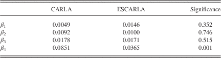
Random functions are generated for the reward function of the games. The functions are generated by the union of Gaussian bells. In order to demonstrate that the performance of the technique is not lowered some single-agent functions are also taken into account. Single-agent functions use one or two bells while multi-agent functions will use between one and six of these bells. The number of bells is generated at random. The parameters of the bells μ ∈ [0, 1] and σ ∈ [0.01, 1] are generated randomly too, as well as the factor f ∈ [0.5, 1] multiplying the factor for the bells to make them different in amplitude. An extra parameter r ∈ [0.75, 0.95] is generated for introducing noise in single-agent settings. Two ways for introducing noise in single-agent setting are explored with these functions, adding noisy bells or randomly selecting between them. The analytical expressions are introduced in (A13) in Appendix B. Notice that β 1, β 2 and β 3 are single-agent problems, while β 4 is the only one representing a game of two players.
In all, 50 games were generated from each type of function. The average linear difference between the global maximum of the function and the final average reward collected by agents over 10 000 time steps are shown in Table 2. The same parameter settings from the previous tests are used. A Wilcoxon test shows that the ESCARLA performs better than the original method for multi-agent games. The results of this test can be seen in the last column of the Table 2.
Mean absolute error
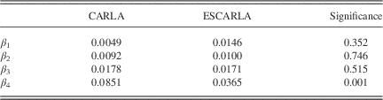
Every row shows the average difference between the long-run reward and the current maximum reward. The first row shows the previous continuous action reinforcement learning automata (CARLA), the second shows results for the exploring selfish continuous action reinforcement learning automaton (ESCARLA) method. ESCARLA considerably reduces the difference for multi-agent games while it does not harm performance in single-agent settings. The last column shows the Wilcoxon test significance.
5.2 Water reservoirs problem
Below, we report a control problem which is a simplified yet representative problem of controlling the water level of a network of connected reservoirs or locks. Typically, such a network is spread over different countries or authorities who want to decide independently on the level of the reservoirs belonging to their territory, yet it is not allowed to get the other ones in situations that would lead to flooding or water scarcity. An example is the Belgian lock systems. Water enters from France and Germany, and within Belgium the locks located in the South are controlled by Wallonia and the locks in the North by Flanders. Controlling reservoirs by RL is not entirely new. In Castelletti et al. (Reference Castelletti, Pianosi and Restelli2012) an RL approach is described for controlling a single reservoir. In this paper, the setting is much more complicated as a network of locks is considered.
Consider two water reservoirs that belong to different provinces. Each reservoir covers the demand of the region. The reservoirs are normally filled by rainfall. Both reservoirs may discharge to the sea using a flow limited by means of a valve. The reservoirs are connected so they can transport water from one to the other. This flow comes at a price that linearly depends on the levels of water of each reservoir, flowing from a high level to a lower one is much cheaper than the other way around. In case of emergency they may also use an external source for feeding or discharging the reservoir. This external resource can only be used when both reservoirs are full or empty to avoid flooding or water scarcity. There is only one connection to the external source that becomes more expensive when used by both reservoirs at the same time. Figure 10 illustrates this problem.
Water reservoirs problem
A more detailed description of the system is given next. Rainfall is normally distributed with mean 0.5 and standard deviation 0.1 in both provinces. The demand is fixed in both provinces at 0.5. Valves controlling water to flow to the sea of both reservoirs allow a maximum flow of 0.35/time unit. The cost of transporting a unit of water from or to the external source is 0.5 if it is used by only one province and 4 when used by the both of them. The cost for transporting water from one province to the other depends on the difference of water levels as shown in Equation (8), where level 1 is the level of the water in the reservoir of the province which is giving the water and level 2 the level of the water of the reservoir of the province which is asking for the water. The objective of this problem is to find the adequate levels of water that the reservoirs should keep to meet the demand at the lowest cost. If a reservoir’s level is higher than the target level, it discharges the water to the other reservoir if the other needs it to reach its target level or to the sea as fast as the valve allows it. The cost is calculated after 50 time units starting from random levels of water at each reservoir. Figure 11 shows a contour representation of the average reward (calculated over a hundred simulations) that the learners may expect when facing this problem (a contour representation to the left and the landscape representation to the right). The expected cost is plotted over the z-axis and the actions runs from completely empty (0) to completely full (1).
 $$cost\,=\,50\left( {level_{2} \,{\minus}\,level_{1} \,{\plus}\,1} \right)$$
The water reservoirs problem. On the left the contour representation of the reward, while on the right its landscape is shown
Note that there are two NE in this problem. The total amount of water in both provinces has to be sufficient to avoid the need for feeding the reservoirs from the external source but not too much to avoid discharging to the external source at a high cost. This is necessary due to the stochasticity of the rainfall. Because it is much more expensive to simultaneously use the external resource for both reservoirs and it is much cheaper to move water from one reservoir to the other if there is a big difference in their levels it is preferable to store most of water in one reservoir and keep the other lower.
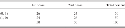
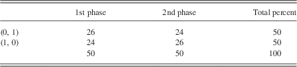
Table 3 shows the percentage of the times that each optimum was found with ESCARLA method at each phase using the same settings as before. Each row represents the percentage of times that the top-left or bottom-right maximum was found. The last row shows that ESCARLA was always successful in finding one of the NE in the first phase and the other one in the second phase. Notice that they find both NE with equal probability, which is to be expected as the problem is symmetric.
Convergence to each optimum per exploration phase
6 Conclusions
In this paper, we propose a distributed RL approach which cannot only deal with continuous actions but also with complex interactions. We show that two agents applying independently an LA update scheme can converge to an NE or even the Pareto optimal NE by extending the ESRL idea. More precisely, we introduce a novel method for estimating the basin of attraction around a locally superior strategy in a common interest game. This allows learners to efficiently explore the action space, by avoiding the basin of attraction of previously discovered attractors. This affirmation is supported by a number of experiments. The new method achieves good results in artificially created functions that represent challenging distributed optimization problems. A control problem inspired by a real-world problem is also introduced and it is shown that our approach successfully solves the problem. We believe that this approach has great potential for the control of complex systems, which are hard to solve analytically. Examples are complex networks such as telecom networks or water reservoir networks. In future work, we plan to study the effect of this technique in games of more than two agents and in conflicting interest games.
Appendix A: Continuous action reinforcement learning automata convergence in continuous action games
The analysis will be performed for normalized reward signals  $$\beta \,{\rm :}\,{\Re } \to[0,\,1]$$
—no generality is lost because any closed interval can be mapped to this interval by a linear transformation. The final goal of this analysis is to find the necessary restrictions to guarantee convergence to local optima.
The sequence of PDF updates is a Markovian process, where for each time step t an action  $a_{t}^{{\left( i \right)}} \in A^{{\left( i \right)}} $
is selected and a new
 $f_{t}^{{\left( i \right)}} $
is returned for every learner i. The expected value
 $\bar{f}_{{t\,{\plus}\,1}}^{{\left( i \right)}} $
of
 $$f_{{t\,{\plus}\,1}}^{{\left( i \right)}} $$
can be computed using following equation:
 $$\bar{f}_{{t{\plus}1}}^{{\left( i \right)}} \left( a \right)=\mathop{\int}\limits_{{\minus}\infty}^{{\plus}\!\infty} {f_{t}^{{\left( i \right)}} } \left( z \right)\ f_{{t{\plus}1}}^{{\left( i \right)}} \left( {a\,\mid\,a_{t}^{{\left( i \right)}} =z} \right)dz$$
Let  $\bar{\gamma }_{t}^{{\left( i \right)}} \,\left( z \right)\,=\,\bar{\gamma }_{t}^{{\left( i \right)}} \!\mid\! a_{t} \,=\,z$
be the expected value for
 $\gamma _{t}^{{\left( i \right)}} $
if
 $a_{t}^{{\left( i \right)}} \,=\,z$
taking into account the other agent policies,
 $\bar{\bar{\gamma }}_{t}^{{\left( i \right)}} $
its expected value and
 $\bar{\beta }_{t}^{{\left( i \right)}} \,\left( z \right)$
the expected value for
 $\beta _{t}^{{\left( i \right)}} \,\left( z \right)$
as shown in (A2). Then (A1) could be rewritten as (A3):
 $$\eqalignno{ \bar{\gamma }_{t}^{{\left( i \right)}} \left( z \right)= & \mathop{\int}\limits_{{\minus}\infty}^{{\plus}\!\infty} \cdots \mathop{\int}\limits_{{\minus}\infty}^{{\plus}\!\infty} {f_{t}^{{\left( 0 \right)}} \left( {z^{{\left( 0 \right)}} } \right) \cdots f_{t}^{{\left( {i{\minus}1} \right)}} \left( {z^{{\left( {i{\minus}1} \right)}} } \right)} \cr & f_{t}^{{\left( {i{\plus}1} \right)}} \left( {z^{{\left( {i{\plus}1} \right)}} } \right) \cdots f_{t}^{{\left( n \right)}} \left( {z^{{\left( n \right)}} } \right) \cr & \left( {\gamma _{t}^{{\left( i \right)}} \!\mid\!a_{t}^{{\left( i \right)}} \,=\,z,a_{t}^{{\left( 0 \right)}} \,=\,z^{{\left( 0 \right)}} , \cdots a_{t}^{{\left( n \right)}} \,=\,z^{{\left( n \right)}} } \right)dz^{{\left( n \right)}} \cdots dz^{{\left( 0 \right)}} \cr \bar{\beta }_{t}^{{\left( i \right)}} \left( z \right)= & \mathop{\int}\limits_{{\minus}\infty}^{{\plus}\!\infty} \cdots \mathop{\int}\limits_{{\minus}\infty}^{{\plus}\!\infty} {f_{t}^{{\left( 0 \right)}} \left( {z^{{\left( 0 \right)}} } \right) \cdots f_{t}^{{\left( {i{\minus}1} \right)}} \left( {z^{{\left( {i{\minus}1} \right)}} } \right)} \cr & f_{t}^{{\left( {i{\plus}1} \right)}} \left( {z^{{\left( {i{\plus}1} \right)}} } \right) \cdots f_{t}^{{\left( n \right)}} \left( {z^{{\left( n \right)}} } \right) \cr & \beta _{t}^{{\left( i \right)}} \left( {z^{{\left( 0 \right)}} , \cdots ,z^{{\left( {i{\minus}1} \right)}} ,z,z^{{\left( {i{\plus}1} \right)}} , \cdots ,z^{{\left( n \right)}} } \right)dz^{{\left( n \right)}} \cdots dz^{{\left( 0 \right)}} \cr \bar{\bar{\gamma }}_{t}^{{\left( i \right)}} & =\mathop{\int}\limits_{{\minus}\infty}^{{\plus}\!\infty} {f_{t}^{{\left( i \right)}} \left( z \right)\bar{\gamma }_{t}^{{\left( i \right)}} \left( z \right)dz} $$
 $$\eqalignno{ \bar{f}_{{t{\plus}1}}^{{\left( i \right)}} \left( a \right)= & \mathop{\int}\limits_{{\minus}\infty}^{{\plus}\!\infty} {f_{t}^{{\left( i \right)}} \left( z \right)\bar{\gamma }_{t}^{{\left( i \right)}} \left( z \right)} \cr & \left( {f_{t}^{{\left( i \right)}} \left( a \right){\plus}\alpha ^{{\left( i \right)}} \bar{\beta }_{t}^{{\left( i \right)}} \left( z \right)e^{{{\minus}{1 \over 2}\left( {{{a{\minus}z} \over {\lambda _{t}^{{\left( i \right)}} }}} \right)^{2} }} } \right)dz \cr & =f_{t}^{{\left( i \right)}} \left( a \right)\bar{\bar{\gamma }}_{t}^{{\left( i \right)}} {\plus} \cr & \alpha ^{{\left( i \right)}} \mathop{\int}\limits_{{\minus}\infty}^{{\plus}\!\infty} {f_{t}^{{\left( i \right)}} \left( z \right)\bar{\gamma }_{t}^{{\left( i \right)}} \left( z \right)\bar{\beta }_{t}^{{\left( i \right)}} \left( z \right)e^{{{\minus}{1 \over 2}\left( {{{a{\minus}z} \over {\lambda _{t}^{{\left( i \right)}} }}} \right)^{2} }} dz} $$
Let us have a look at the right member of the integral.  $f_{t}^{{\left( i \right)}} \,\left( z \right)$
is multiplied by the factor composed by the normalization factor given that
 $$a_{t}^{{\left( i \right)}} = z$$
, the feedback signal
 $\bar{\beta }_{t}^{{\left( i \right)}} \,\left( z \right)$
and the distance measure
 $e^{{{\minus}{1 \over 2}\left( {{{a{\minus}z} \over {\lambda _{t}^{{\left( i \right)}} }}} \right)^{2} }} $
which can be interpreted as the strength of the relation of actions a and z, the higher the value of this product, the bigger the relation of these actions. Let us call this composed factor
 $G_{t}^{{\left( i \right)}} \,\left( {a,\,z} \right)$
and
 $\bar{G}_{t}^{{\left( i \right)}} \,\left( a \right)$
its expected value at time step t with respect to z. Then Equation (A3) could be finally formulated as (A4):
 $$\eqalignno{ \bar{f}_{{t{\plus}1}}^{{\left( i \right)}} \left( a \right) & =f_{t}^{{\left( i \right)}} \left( a \right)\bar{\bar{\gamma }}_{t}^{{\left( i \right)}} {\plus}\alpha ^{{\left( i \right)}} \bar{G}_{t}^{{\left( i \right)}} \left( a \right) \cr & =f_{t}^{{\left( i \right)}} \left( a \right)\left( {\bar{\bar{\gamma }}_{t}^{{\left( i \right)}} {\plus}{{\alpha ^{{\left( i \right)}} \bar{G}_{t}^{{\left( i \right)}} \left( a \right)} \over {f_{t}^{{\left( i \right)}} \left( a \right)}}} \right) $$
The sign of the first derivative of  $f_{t}^{{\left( i \right)}} $
depends on the factor
 $\bar{\bar{\gamma }}_{t}^{{\left( i \right)}} {\plus}{{\alpha ^{{\left( i \right)}} \bar{G}_{t}^{{\left( i \right)}} \,\left( a \right)} \over {f_{t}^{{\left( i \right)}} \,\left( a \right)}}$
of expression (A4) so it behaves as shown in (A5):
 $${{\partial f_{t}^{{\left( i \right)}} } \over {\partial t}}\left\{ {\matrix{ {\lt \,0} & {\bar{\bar{\gamma }}_{t}^{{\left( i \right)}} {\plus}{{\alpha ^{{\left( i \right)}} \bar{G}_{t}^{{\left( i \right)}} \left( a \right)} \over {f_{t}^{{\left( i \right)}} \left( a \right)}}\,\lt\, 1} \cr {=0} & {\bar{\bar{\gamma }}_{t}^{{\left( i \right)}} {\plus}{{\alpha ^{{\left( i \right)}} \bar{G}_{t}^{{\left( i \right)}} \left( a \right)} \over {f_{t}^{{\left( i \right)}} \left( a \right)}}\,=\!1} \cr {\gt \,0} & {\bar{\bar{\gamma }}_{t}^{{\left( i \right)}} {\plus}{{\alpha ^{{\left( i \right)}} \bar{G}_{t}^{{\left( i \right)}} \left( a \right)} \over {f_{t}^{{\left( i \right)}} \left( a \right)}}\,\gt\, 1} \cr } } \right.$$
Notice  $\bar{\bar{\gamma }}_{t}^{{\left( i \right)}} $
is a constant for all a ∈ A (i) and
 $\mathop{\int}\limits_{{\minus}\infty}^{{\plus}\!\infty} {f_{t}^{{\left( i \right)}} \left( z \right)\,dz=1} $
so:
 $$\eqalignno{ & \exists _{{b_{1}^{{\left( i \right)}} ,b_{2}^{{\left( i \right)}} \in A^{{\left( i \right)}} }} :{{\bar{G}_{t}^{{\left( i \right)}} \left( {b_{1}^{{\left( i \right)}} } \right)} \over {f_{t}^{{\left( i \right)}} \left( {b_{1}^{{\left( i \right)}} } \right)}}\,\ne\,{{\bar{G}_{t}^{{\left( i \right)}} \left( {b_{2}^{{\left( i \right)}} } \right)} \over {f_{t}^{{\left( i \right)}} \left( {b_{2}^{{\left( i \right)}} } \right)}}\Rightarrow \cr & \exists _{{A_{{\plus}}^{{\left( i \right)}} ,\, A_{{\minus}}^{{\left( i \right)}} \,\subset\,A^{{\left( i \right)}} ,\,A_{{\plus}}^{{\left( i \right)}} {\cap}A_{{\minus}}^{{\left( i \right)}} \,=\,{\emptyset} }}{\vskip 3pt ,}\forall _{{a_{{\plus}}^{{\left( i \right)}} \in A_{{\plus}}^{{\left( i \right)}} ,a_{{\minus}}^{{\left( i \right)}} \in A_{{\minus}}^{{\left( i \right)}} }} : \cr & \left( {{{\partial f_{t}^{{\left( i \right)}} \left( {a_{{\plus}}^{{\left( i \right)}} } \right)} \over {\partial t}}\,\gt\, 0} \right)\wedge\left( {{{\partial f_{t}^{{\left( i \right)}} \left( {a_{{\minus}}^{{\left( i \right)}} } \right)} \over {\partial t}}\,\lt \,0} \right) $$
From logical implication (A6) it can be assured that the sign of  ${{\partial f_{t}^{{\left( i \right)}} \,\left( a \right)} \over {\partial t}}$
will be determined by the ratio
 ${{\bar{G}_{t}^{{\left( i \right)}} \,\left( a \right)} \over {f_{t}^{{\left( i \right)}} \,\left( a \right)}}$
. Notice subsets
 $A_{{\plus}}^{{\left( i \right)}} $
and
 $A_{{\minus}}^{{\left( i \right)}} $
are composed by the elements of A (i) that have not reached their value for the PDF in equilibrium with
 $\bar{G}_{t}^{{\left( i \right)}} \,\left( a \right)$
. That is, the
 $A_{{\plus}}^{{\left( i \right)}} $
subset is composed by all a ∈ A (i) having a value of PDF which is too small with respect to
 $\bar{G}_{t}^{{\left( i \right)}} \left( a \right)$
and vice versa for
 $A_{{\minus}}^{{\left( i \right)}} $
.
Let  $a_{{\asterisk}}^{{\left( i \right)}} \in A^{{\left( i \right)}} $
be the actions yielding the highest value for every agent i at expression
 $\mathop{\int}\nolimits_{{\minus}\infty}^{{\plus}\infty} {\bar{\beta }_{t}^{{\left( i \right)}} \left( z \right)e^{{{\minus}{1 \over 2}\left( {{{a{\minus}z} \over {\lambda _{t}^{{\left( i \right)}} }}} \right)^{2} }} dz} $
as shown in (A7). It is important to stress that
 $a_{{\asterisk}}^{{\left( i \right)}} $
are not the optimum of
 $\bar{\beta }_{t}^{{\left( i \right)}} $
given the set
 $f_{t}^{{\left( j \right)}} $
but the points yielding the optimal vicinity around it and defined by
 $e^{{{\minus}{1 \over 2}\left( {{{a_{{\asterisk}}^{{\left( i \right)}} {\minus}z} \over {\lambda _{t}^{{\left( i \right)}} }}} \right)^{2} }} $
which depends on
 $\lambda _{t}^{{\left( i \right)}} $
:
 $$\forall _{{a\in A^{{\left( i \right)}} }} \mathop{\int}\limits_{{\minus}\infty}^{{\plus}\!\infty} {\bar{\beta }_{t}^{{\left( i \right)}} \left( z \right)e^{{{\minus}{1 \over 2}\left( {{{a_{{\asterisk}}^{{\left( i \right)}} {\minus}z} \over {\lambda _{t}^{{\left( i \right)}} }}} \right)^{2} }} dz \,⩾ \, \mathop{\int}\limits_{{\minus}\infty}^{{\plus}\!\infty} {\bar{\beta }_{t}^{{\left( i \right)}} \left( z \right)e^{{{\minus}{1 \over 2}\left( {{{a{\minus}z} \over {\lambda _{t}^{{\left( i \right)}} }}} \right)^{2} }} dz} } $$
For symmetric games, that is common interest games ( $\forall _{{i,j}} :\beta _{t}^{{\left( i \right)}} =\beta _{t}^{{\left( j \right)}} $
), all
 $a_{{\asterisk}}^{{\left( i \right)}} $
will correspond initially to the same maximum in the joint-action space, if all learner start with the same parameters and an uniform PDF each one. Then (A8) holds:
 $$\matrix{ {\forall _{t} :f_{t}^{{\left( i \right)}} \left( {a_{{\asterisk}}^{{\left( i \right)}} } \right)\,\,⩾ \,\, f_{t}^{{\left( i \right)}} \left( {a^{{\left( i \right)}} } \right)} \hfill & \!\!\!\!\!{\Rightarrow f_{{t{\plus}1}}^{{\left( i \right)}} \left( {a_{{\asterisk}}^{{\left( i \right)}} } \right) \,\,\,⩾ \, \, f_{{t{\plus}1}}^{{\left( i \right)}} \left( {a^{{\left( i \right)}} } \right)} \hfill \cr {\forall _{t} :\bar{\beta }_{t}^{{\left( i \right)}} \left( {a_{{\asterisk}}^{{\left( i \right)}} } \right) \,\,⩾ \,\,\beta _{t}^{{\left( i \right)}} \left( {a^{{\left( i \right)}} } \right)} \hfill & \!\!\!\!\!{\Rightarrow\bar{\beta }_{{t{\plus}1}}^{{\left( i \right)}} \left( {a_{{\asterisk}}^{{\left( i \right)}} } \right) \,\,⩾ \, \, \bar{\beta }_{{t{\plus}1}}^{{\left( i \right)}} \left( {a^{{\left( i \right)}} } \right)} \hfill \cr {\forall _{t} :\bar{G}_{t}^{{\left( i \right)}} \left( {a_{{\asterisk}}^{{\left( i \right)}} } \right) \,⩾ \,\,\bar{G}_{t}^{{\left( i \right)}} \left( {a^{{\left( i \right)}} } \right)} \hfill & \!\!\!\!\!{\Rightarrow\bar{G}_{{t{\plus}1}}^{{\left( i \right)}} \left( {a_{{\asterisk}}^{{\left( i \right)}} } \right) \,⩾ \, \, \bar{G}_{{t{\plus}1}}^{{\left( i \right)}} \left( {a^{{\left( i \right)}} } \right)} \hfill \cr } $$
As the first derivative of the PDF depends on  ${{\bar{G}_{t}^{{\left( i \right)}} \left( a \right)} \over {f_{t}^{{\left( i \right)}} \left( a \right)}}$
the value necessary for keeping
 ${{\partial f_{t}^{{\left( i \right)}} \left( a \right)} \over {\partial t}}=0$
is also the highest for every
 $a_{{\asterisk}}^{{\left( i \right)}} $
.
Notice that the maximum update that  $f_{t}^{{\left( i \right)}} \left( {a_{{\asterisk}}^{{\left( i \right)}} } \right)$
may receive is obtained when
 $a_{t}^{{\left( i \right)}} =a_{{\asterisk}}^{{\left( i \right)}} $
—centering the bell at
 $a_{{\asterisk}}^{{\left( i \right)}} $
— then if
 $f_{t}^{{\left( i \right)}} \left( {a_{{\asterisk}}^{{\left( i \right)}} } \right)$
reaches the value
 ${1 \over {\lambda _{t}^{{\left( i \right)}} \sqrt {2\pi } }}$
, its first derivative will not be higher than 0 as shows (A9) as
 $\beta {\rm :}\Re \to[0,1]$
 $$\eqalignno{ f_{{t{\plus}1}}^{{\left( i \right)}} \left( {a_{{\asterisk}}^{{\left( i \right)}} } \right) =& \,\bar{\gamma }_{t}^{{\left( i \right)}} \left( {a_{t}^{{\left( i \right)}} } \right) \cr & \left( {f_{{\asterisk}}^{{\left( i \right)}} \left( {a_{t}^{{\left( i \right)}} } \right){\plus}\beta _{t}^{{\left( i \right)}} \left( {a_{t}^{{\left( i \right)}} } \right)\alpha ^{{\left( i \right)}} e^{{{\minus}{1 \over 2}\left( {{{a_{{\asterisk}}^{{\left( i \right)}} {\minus}a_{t}^{{\left( i \right)}} } \over {\lambda _{t}^{{\left( i \right)}} }}} \right)^{2} }} } \right) \cr & \,⩽ \, {1 \over {1{\plus}\alpha ^{{\left( i \right)}} \lambda _{t}^{{\left( i \right)}} \sqrt {2\pi } }}\left( {{1 \over {\lambda _{t}^{{\left( i \right)}} \sqrt {2\pi } }}{\plus}\alpha ^{{\left( i \right)}} } \right) \cr & \,⩽ \, {1 \over {1{\plus}\alpha ^{{\left( i \right)}} \lambda _{t}^{{\left( i \right)}} \sqrt {2\pi } }}\left( {{{1{\plus}\alpha ^{{\left( i \right)}} \lambda _{t}^{{\left( i \right)}} \sqrt {2\pi } } \over {\lambda _{t}^{{\left( i \right)}} \sqrt {2\pi } }}} \right) \cr & \,⩽ \, {1 \over {\lambda _{t}^{{\left( i \right)}} \sqrt {2\pi } }} $$
Then the equilibrium point of  $f_{t}^{{\left( i \right)}} \left( {a_{{\asterisk}}^{{\left( i \right)}} } \right)$
has the higher bound
 ${1 \over {\lambda _{t}^{{\left( i \right)}} \sqrt {2\pi } }}$
. Notice that the closer the
 $\beta _{t}^{{\left( i \right)}} \left( {a_{{\asterisk}}^{{\left( i \right)}} } \right)$
to 1, the closer the equilibrium point of
 $f_{t}^{{\left( i \right)}} \left( {a_{{\asterisk}}^{{\left( i \right)}} } \right)$
to its higher bound:
 $${{\partial f_{t}^{{\left( i \right)}} \left( {a_{{\asterisk}}^{{\left( i \right)}} } \right)} \over {\partial t}}\left\{ {\matrix{ {\lt \,0} & {f_{t}^{{\left( i \right)}} \left( {a_{{\asterisk}}^{{\left( i \right)}} } \right)\gt {1 \over {\lambda _{t}^{{\left( i \right)}} \sqrt {2\pi } }}} \cr {=0} & {f_{t}^{{\left( i \right)}} \left( {a_{{\asterisk}}^{{\left( i \right)}} } \right)={1 \over {\lambda _{t}^{{\left( i \right)}} \sqrt {2\pi } }}} \cr {\gt \,0} & {f_{t}^{{\left( i \right)}} \left( {a_{{\asterisk}}^{{\left( i \right)}} } \right)\lt {1 \over {\lambda _{t}^{{\left( i \right)}} \sqrt {2\pi } }}} \cr } } \right.$$
We can conclude from (A10) that the highest value for f (i) will be achieved at  $a_{{\asterisk}}^{{\left( i \right)}} $
as shown in (A11) which has the higher bound
 ${1 \over {\lambda _{t}^{{\left( i \right)}} \sqrt {2\pi } }}$
:
 $$\eqalignno{ \forall _{{a\in A^{{\left( i \right)}} \,\backslash\,\{ a_{{\asterisk}}^{{\left( i \right)}} \} }} : & {\rm lim}_{{t\to\infty}} \,f_{t}^{{\left( i \right)}} \left( a \right)\,\,\lt \,\,f_{t}^{{\left( i \right)}} \left( {a_{{\asterisk}}^{{\left( i \right)}} } \right) \cr & {\rm lim}_{{t\to\infty}} \,f_{t}^{{\left( i \right)}} \left( {a_{{\asterisk}}^{{\left( i \right)}} } \right)\,⩽ \, {1 \over {\lambda _{t}^{{\left( i \right)}} \sqrt {2\pi } }} $$
Finally,
 $$\matrix{ \hfill {\lim _{{\lambda ^{{\left( i \right)}} \downarrow0}} \lim _{{t\to\infty}} f_{t}^{{\left( i \right)}} \left( {a_{{\asterisk}}^{{\left( i \right)}} } \right)} \hfill \! \! \! \! \! \! \! \! \! \! {=\! & \infty} \cr \hfill {\forall _{{a\,\ne\,a_{{\asterisk}}^{{\left( i \right)}} }} :\lim _{{\lambda ^{{\left( i \right)}} \downarrow0}} \lim _{{t\to\infty}} f_{t}^{{\left( i \right)}} \left( a \right)} \hfill \,{=& 0} \cr } $$
We can safety conclude that the set of CARLA will converge to an equilibrium in the joint-action space as long as the parameter α is low enough for the learners to match their expected policies through time. Which of the multiple equilibria is selected will depend on the initialization of the parameter λ.
Appendix B: Analytical expression of rewards
$$\eqalignno{ \beta \left( {a^{{\left( 1 \right)}} ,a^{{\left( 2 \right)}} } \right) & ={\rm Bell}\left( {a^{{\left( 1 \right)}} ,a^{{\left( 2 \right)}} ,0.5,0.5,0.084} \right) \cr & {\bigcup }0.63\:{\rm Bell}\left( {a^{{\left( 1 \right)}} ,a^{{\left( 2 \right)}} ,0.1,0.9,0.187} \right) \cr & {\bigcup}0.63\:{\rm Bell}\left( {a^{{\left( 1 \right)}} ,a^{{\left( 2 \right)}} ,0.9,0.1,0.187} \right) \cr \beta ^{i} \left( {a_{t}^{{\left( 1 \right)}} ,a_{t}^{{\left( 2 \right)}} } \right) & =0.3125\left( {1{\plus}{\rm sin}(9a_{t}^{{\left( 1 \right)}} a_{t}^{{\left( 2 \right)}} )} \right)^{2} {{a_{t}^{{\left( 1 \right)}} {\plus}a_{t}^{{\left( 2 \right)}} } \over 2} \cr \beta ^{{ii}} \left( {a_{t}^{{\left( 1 \right)}} ,a_{t}^{{\left( 2 \right)}} } \right) & ={\rm Bell}\left( {\left( {a_{t}^{{\left( 1 \right)}} } \right)^{2} ,a_{t}^{{\left( 2 \right)}} ,0.5,0.5,0.002} \right) \cr & {\bigcup}0.7\:{\rm Bell}\left( {\left( {a_{t}^{{\left( 1 \right)}} } \right)^{2} ,a_{t}^{{\left( 2 \right)}} ,0.1,0.1,0.2} \right) \cr & {\bigcup}0.7\:{\rm Bell}\left( {\left( {a_{t}^{{\left( 1 \right)}} } \right)^{2} ,a_{t}^{{\left( 2 \right)}} ,0.9,0.9,0.2} \right) \cr & {\bigcup}0.7\:{\rm Bell}\left( {\left( {a_{t}^{{\left( 1 \right)}} } \right)^{2} ,a_{t}^{{\left( 2 \right)}} ,0.9,0.1,0.2} \right) \cr & {\bigcup}0.7\:{\rm Bell}\left( {\left( {a_{t}^{{\left( 1 \right)}} } \right)^{2} ,a_{t}^{{\left( 2 \right)}} ,0.1,0.9,0.2} \right) \cr \beta _{1} \left( a \right) & =\mathop{{\cup}}\limits_{{i=1}}^{n} f_{i} \:b_{i} \left( a \right) \cr \beta _{2} \left( a \right) & =\mathop{{\cup}}\limits_{{i=1}}^{n} \left( {r_{i} \:f_{i} \:b_{i} \left( a \right){\plus}{\rm rand}\left( {1{\minus}r_{i} } \right)} \right) \cr \beta _{3} \left( a \right) & ={\rm pick}\left\{ {{{r_{i} } \over {\mathop{\sum}\limits_1^n r_{i} }},f_{i} \:b_{i} \left( a \right)} \right\} \cr \beta _{4} \left( {a^{{\left( 1 \right)}} ,a^{{\left( 2 \right)}} } \right) & =\mathop{{\cup}}\limits_{{i=1}}^{n} f_{i} {\rm Bell}_{i} \left( {a^{{\left( 1 \right)}} ,a^{{\left( 2 \right)}} } \right) \cr & \hskip -39pt b(a) =e{\minus}{{(a{\minus}\mu )^{2} } \over {2\sigma ^{2} }}\qquad \cr & \hskip -50pt \quad {\rm Bell}\left( {a^{{\left( 1 \right)}} ,a^{{\left( 2 \right)}} ,\mu ^{{(2)}} ,\sigma } \right) =e^{{{\minus}{{\left( {a^{{(1)}} {\minus}\mu ^{{(1)}} } \right)^{2} {\plus}\left (a^{{(2)}} {\minus}\mu ^{{(2)}} \right)^2 } \over {2\sigma ^{2} }}}} \cr & \hskip -39pt a{\cup}b =a{\plus}b{\minus}ab $$