2. Structure characteristics and operation principle

The hybrid hand’s structure, shown in Figure 1a, consists of a base, three finger plane limbs and a flexible closed-loop chain. The finger plane limb is composed of a motor, a screw rod, a slider, one long link, an inner short link, an outer short link, an inner finger link and a finger link. The flexible closed-loop chain is composed of three flexible linkages and three rotating shaft rods. The flexible linkages include an adjustable nut, a spring, an outer sleeve rod, an inner rod, an end cover and an inner end cover. The structure and working principle of the hybrid hand are explained as follows:

Figure 1.

Hybrid hand structure and its topology diagram. (a) A 3D model of the hybrid hand. (b) The grasping limit pose of the hybrid hand prototype. (c) Topology diagram of hybrid hand.

Let R and P be the revolute joint and the prismatic joint. Let (||, ⊥, |) be the parallel constraint, perpendicular constraint and collinear constraint. The motor with a screw rod is fixed onto the base. In the finger plane limb, the slider is driven by the screw rod of the motor and moved along the guide slot of the base. The slider and the long link, the base and the inner short link, the long link and the outer short link, the long link and the inner short link, the long link and the inner short link, the long link and the inner short link, the outer short link and the finger link, the finger link and the inner short link are all connected by the R joint, and all the R joints in the finger plane limb are parallel. The rotating shaft rod with the outer short link and the finger link are also connected by the R joint. The S joint in flexible closed-loop chain connects the flexible linkage and the two ends of the rotating shaft rod. The flexible closed-loop chain’s inner rod and outer sleeve rod are collinear through the axis, and the P joint connects the two. The spring axis is collinear with the axis of the inner rod and the outer sleeve rod, and the spring surface can move relative to the surface of the two rods. The two ends of the spring are fixedly connected to the inner end cover, the outer rod is fixedly connected to the end cover, and the inner rod is fixedly connected to the inner end cover. At the same time, the initial length and the size of the spring can be adjusted by adjusting the position of the adjustable nut relative to the inner rod. The finger link contains a force sensor for measuring the value of the contact force, and the two parts composed of the finger link are fixed and connected with the two ends of the force sensor through screw threads, which is regarded as a link in the theoretical analysis.

In the theoretical model, the two ends of the flexible linkage and the rotation shaft rod are connected by S joints. However, in order to enhance the tensile capacity between the flexible linkage and the rotation shaft rod in the hybrid coupling prototype, the S joint is treated as an equivalent combination of an R joint and a U joint. The R joint is situated within the flexible linkage, allowing the inner rod and the outer sleeve rod to rotate relative to each other. Their rotation direction is along the axial direction of the flexible linkage, with the axis of the R joint aligned with the center of the U joint, ensuring that its motion characteristics are the same as the S joint. To simplify the theoretical model diagram, S joints are used in place of the R and U joints during the analysis, which does not impact the kinematics. Furthermore, since the forces acting on the grasped object are the primary focus of the dynamic analysis, this equivalence does not affect the results of the dynamic calculations either.

The hybrid hand incorporates an internal force sensor. The image of the sensor and the principle for measuring fingertip contact force are shown in Figure 1. When the hybrid hand grasps an object, a contact force is generated at the fingertip, which is transmitted through the fingertip link and the R joint. This contact force acts on the force sensor, resulting in a positive correlation between the two values. Based on the measurement data from the force sensor, the fingertip contact force can be calculated and obtained, which can be used to evaluate the mass of the grasped object and provide the hardware basis for the control of the hybrid hand. The sensor has a measurement range of 0 to 10 kg, an accuracy of 0.1%, and dimensions of 19 mm × 16 mm × 6 mm.

By controlling the motor to drive the screw rotation to make the slider slide along the screw axis in the guide groove of the base, the finger plane limb to bend and extend. When the fingertip and the object contact, the contact force will be transmitted to the spring along the finger link and the rotating shaft rod, so that the spring is compressed, to avoid the fingertip and the object’s rigid contact to produce impact force and destroy the object. This feature enables the hybrid hand to grasp various objects. When the hybrid hand grips a heavy object, three fingertips contact the object, and the finger limb with the object forms a closed-loop chain to ensure the stability and safety of grasping. The flexible closed-loop chain shares a part of the load so that the hybrid hand has a large bearing capacity. At this time, the force of the spring depends on the pose of the hybrid hand to grasp the object. The limit pose of the fingertip closure of the hybrid hand prototype is shown in Figure 1b. The topology diagram of the hybrid hand is shown in Figure 1c.

2.1. Degree of freedom analysis

Since there is a substantial number of links in the hybrid hand, the splitting method can be used to calculate the DOFs of the hybrid hand. The calculation process is as follows: First, determine the DOFs of the finger plane limbs, and then calculate the overall DOFs of the hybrid hand. When a single finger limb moves in a plane, the M_fi of its in-plane motion is calculated as follows:

(1) \begin{equation} M_{fi}=3\left(n_{fli}-n_{fji}-1\right)+\sum f=3\times \left(7-8-1\right)+8=2 \end{equation}

here, n_fli is the number of rods contained in a single finger plane limb, n_fji is the number of joints contained in a single finger limb, and Σf is the total sum of joints. n_fli = 7 is base, slider and l_ij (j = 1,2,3,4,5) in finger limb i, n_fji = 8, including seven rotating joints and one prismatic joint, and Σf = 8 × 1 = 8.

When the spring in the flexible linkage does not deform, the flexible linkage is equivalent to a single rod, and the overall freedom M of the hybrid hand is calculated as follows:

(2) \begin{equation} M=3\times M_{fi}+6\times n_{l}-3\times n_{j}-\upsilon =3\times M_{f}+6\times 3-3\times 6-3=6+18-18-3=3 \end{equation}

here, n_l is the number of rods contained in the flexible closed-loop chain, n_j is the number of joints contained in a single finger limb and υ is the passive DOF. When the rotating shaft rod in the flexible closed-loop chain is fixedly connected with the finger link or the outer short link, the kinematics of the hybrid hand is not affected. When it is regarded as a fixed connection, n_l = 3 is the number of flexible linkages l_si(i = 1,2,3) contained in the flexible closed-loop chain, n_j = 6 is the number of S joints and υ = 3 is the rotation around the axis of flexible linkage l_si, a passive rotation generated by S joints at both ends of l_si. The results of Eq. (2) prove that the hybrid hand mechanism is a 3-DOF mechanism, and the hybrid hand can be completely controlled by three motors.

When the contact force appears between the fingertip and the object, the spring in the flexible linkage will be compressed by force, and the inner rod and the outer sleeve rod at the ends of the spring are equivalent to the P joint connection, increasing the DOF of the hybrid hand. The DOF of the hybrid hand is greater than the number of motors, making the hybrid hand an underactuated mechanism. This underactuated feature enables the hybrid hand to grasp objects of various shapes and ensures the safety of fingertip contact with the object.

When the three fingers are in contact with the object, each finger limb is similar to the RPS limb and forms a closed loop chain with the object to be grasped, which can be equivalent to a 3RPS parallel mechanism, and the overall DOF is still consistent with the number of motors.

3. Kinematics analysis of hybrid hand fingertips

The kinematics analysis of the hybrid hand can be divided into two stages. In the first stage, the hybrid hand is controlled to reach the predetermined position and ensure contact between the fingertips and the object, and then the second stage is reached. In the second stage, the hybrid hand’s fingertips maintain contact with the object and grasp the object for movement.

3.1. Position analysis of hybrid hand fingertips

The kinematics analysis model of the hybrid hand is shown in Figure 2.

Figure 2.

Kinematics model of single finger and hybrid hand mechanism. (a) Kinematics model of finger plane limb. (b) Kinematics model of hybrid hand mechanism.

As shown in Figure 2a, let {ti} be the coordinate system of axis ti-xyz at finger i at point O, in the finger plane limb i, let each link be named l_ij (i = 1,2,3, j = 1,2,3,4,5). In the finger plane limb, the angle between l_ij and tix in the finger plane is θ _ij (i = 1,2,3,4,5). The fingertip points are p_i, and the positions of each joint are {B_i, D_i, M_i, Q_i, W_i, b_i}. The position of the rotating shaft rod in the flexible closed-loop chain is l_bi (i = 1,2,3), the flexible linkage is l_si (i = 1,2,3) and the position of each link is shown in Figure 2b. The flexible closed-loop chain is connected with finger plane limb i at b_i, so that the flexible linkage and the rotating shaft rod in the flexible closed-loop chain are connected at the point (b _i1, b _i1) through S joint. Let {B} be a coordinate system O-XYZ fixed on B at central point O of base. Let {d_i, v_di, a_di (i = 1,2,3)} be the input displacement, velocity and acceleration of the hybrid hand.

Let ${}_{ti}^{B}{{{\boldsymbol{R}}}}{}$ be a rotation matrix from {ti} to {B}, ${}_{ti}^{B}{{{\boldsymbol{R}}}}{}$ (i = 1,2,3) are derived as follows:

(3) \begin{equation} {}_{t1}^{B}{{{\boldsymbol{R}}}}{}=\dfrac{1}{2}\left(\begin{array}{ccc} -\sqrt{3} &\quad -1 &\quad 0\\[4pt] 1 &\quad -\sqrt{3} &\quad 0\\[4pt] 0 &\quad 0 &\quad 2 \end{array}\right),{}_{t2}^{B}{{{\boldsymbol{R}}}}{}=\left(\begin{array}{ccc} 0 &\quad 1 &\quad 0\\[4pt] -1 &\quad 0 &\quad 0\\[4pt] 0 &\quad 0 &\quad 1 \end{array}\right),{}_{t3}^{B}{{{\boldsymbol{R}}}}{}=\dfrac{1}{2}\left(\begin{array}{ccc} \sqrt{3} &\quad -1 &\quad 0\\[4pt] 1 &\quad \sqrt{3} &\quad 0\\[4pt] 0 &\quad 0 &\quad 2 \end{array}\right) \end{equation}

The vector R_i (i = 1,2,3) of the R joint in finger i of each finger plane limb is derived as follows:

(4) \begin{equation} {{\boldsymbol{R}}}_{1}=\dfrac{1}{2}\left(\begin{array}{c} -1\\[4pt] -\sqrt{3}\\[4pt] 0 \end{array}\right),{{\boldsymbol{R}}}_{2}=\left(\begin{array}{c} 1\\[4pt] 0\\[4pt] 0 \end{array}\right),{{\boldsymbol{R}}}_{3}=\dfrac{1}{2}\left(\begin{array}{c} -1\\[4pt] \sqrt{3}\\[4pt] 0 \end{array}\right) \end{equation}

In the finger plane, two geometric relations in the closed loop formed by links (d_i, l _i1, l _i2) and the relationship between (θ _i2, θ _i1) are obtained as follows:

(5) \begin{equation} -\left(d_{i}-E\right)+l_{i21}\cos \theta _{i2}=l_{i1}\cos \theta _{i1},l_{i21}\sin \theta _{i2}=l_{i1}\sin \theta _{i1}\rightarrow \theta _{i1}=\text{acsin}\left(l_{i21}\sin \theta _{i2}\big/l_{i1}\right) \end{equation}

The relationship between d_i and θ _i2 can be obtained from Eq. (5) as follows:

(6) \begin{equation} \left(d_{i}-E\right)^{2}-2\left(d_{i}-E\right)l_{i21}\cos \theta _{i2}+l_{i21}^{2}=l_{i1}^{2},\cos \theta _{i2}=\dfrac{\left(d_{i}-E\right)^{2}+l_{i21}^{2}-l_{i1}^{2}}{2\left(d_{i}-E\right)l_{i21}} \end{equation}

Let (b_i, ^tib_i) be the position vector of b_i in {B} and {ti}, a relation formula between (b_i, d_i, θ _i2, θ _i3) is derived as follows:

(7) \begin{equation} -d_{i}+l_{i21}\cos \theta _{i2}+l_{i3}\cos \theta _{i3}={}^{ti}{b}{_{ix}^{}},{}^{ti}{b}{_{iz}^{}}=0,l_{i21}\sin \theta _{i2}+l_{i3}\sin \theta _{i3}={}^{ti}{b}{_{iz}^{}},{{\boldsymbol{b}}}_{i}={}_{ti}^{B}{{{\boldsymbol{R}}}}{}{}^{ti}{{{\boldsymbol{b}}}}{_{i}^{}},l_{i}^{2}={}^{ti}{b}{_{ix}^{2}}+{}^{ti}{b}{_{iz}^{2}} \end{equation}

The relationship between (b_i, d_i, θ _i3) is known by substituting these relations into Eq. (7) according to the relationship between d_i and θ _i2 in Eq. (6).

According to b_i and given the values of l _bi1 and l _bi2, b_i1 and b_i2 can be obtained as follows:

(8) \begin{equation} {{\boldsymbol{l}}}_{bi1}={{\boldsymbol{b}}}_{i1}-{{\boldsymbol{b}}}_{i},{{\boldsymbol{l}}}_{bi2}={{\boldsymbol{b}}}_{i2}-{{\boldsymbol{b}}}_{i},{{\boldsymbol{l}}}_{bi1}={{\boldsymbol{R}}}_{i}l_{bi1},{{\boldsymbol{l}}}_{bi2}=-{{\boldsymbol{R}}}_{i}l_{bi1}=-{{\boldsymbol{R}}}_{bi2}l_{bi1} \end{equation}

Before the hybrid hand grasps the object, the spring does not deform, the spring length is the initial length, l_si = l _s0, and the geometric constraints are as follows:

(9) \begin{equation} {{\boldsymbol{l}}}_{s1}={{\boldsymbol{b}}}_{31}-{{\boldsymbol{b}}}_{22},{{\boldsymbol{l}}}_{s20}={{\boldsymbol{b}}}_{11}-{{\boldsymbol{b}}}_{32},{{\boldsymbol{l}}}_{s3}={{\boldsymbol{b}}}_{21}-{{\boldsymbol{b}}}_{12},\left| {{\boldsymbol{l}}}_{si}\right| =l_{si0} \end{equation}

Two geometric relations in the closed loop formed by links (l _i22, l _i3, l _i4, l _i5) are obtained as follows:

(10) \begin{equation} l_{i3}\cos \theta _{i3}+l_{i51}\cos \theta _{i5}=l_{i22}\cos \theta _{i2}+l_{i4}\cos \theta _{i4},\,l_{i3}\sin \theta _{i3}+l_{i51}\sin \theta _{i5}=l_{i22}\sin \theta _{i2}+l_{i4}\sin \theta _{i4} \end{equation}

The relationship between (θ _i2, θ _i3, θ _i5)can be derived from Eq. (10) as follows:

(11) \begin{equation} l_{i3}^{2}+l_{i51}^{2}+l_{i22}^{2}+2\left[l_{i3}l_{i51}\cos \left(\theta _{i3}-\theta _{i5}\right)-l_{i22}l_{i3}\cos \left(\theta _{i2}-\theta _{i3}\right)-l_{i22}l_{i51}\cos \left(\theta _{i2}-\theta _{i5}\right)\right]=l_{i4}^{2} \end{equation}

Let (p_i, ^tip_i) be the position vector of the fingertip at {B} and {ti}, a relation formula between (p_i, d_i, θ _i2, θ _i3, θ _i5) is derived as follows:

(12) \begin{equation} \begin{array}{c} -d_{i}+l_{i21}\cos \theta _{i2}+l_{i3}\cos \theta _{i3}+l_{i5}\cos \theta _{i5}={}^{ti}{p}{_{ix}^{}},{}^{ti}{p}{_{iy}^{}}=0,l_{i21}\sin \theta _{i2}+l_{i3}\sin \theta _{i3}+l_{i5}\sin \theta _{i5}={}^{ti}{p}{_{iz}^{}},\\[4pt] {{\boldsymbol{p}}}_{i}={}_{ti}^{B}{{{\boldsymbol{R}}}}{}{}^{ti}{{{\boldsymbol{p}}}}{_{i}^{}},{{\boldsymbol{p}}}_{i}=\left(\begin{array}{ccc} p_{ix} & p_{iy} & p_{iz} \end{array}\right),{}^{ti}{{{\boldsymbol{p}}}}{_{i}^{}}={}^{ti}{\left(\begin{array}{ccc} p_{ix} & p_{iy} & p_{iz} \end{array}\right)}{} \end{array} \end{equation}

Given the value of d_i, θ _i2 can be obtained according to Eq. (6), the value of θ _i3 and b_i can be obtained by substituting the value of d_i and θ _i2 into Eqs. (7)–(9), and the values of θ _i2 and θ _i3 can be obtained by substituting the value of θ _i5 into Eq. (11). The value of p_i is obtained by substituting the value of (d_i, θ _i2, θ _i3, θ _i5) into Eq. (12).

3.2. Velocity analysis of hybrid hand fingertips and Jacobian vector

To establish the dynamic model of the hybrid hand, the formulas for solving the velocity of several key links of the finger mechanism must be derived. Let v_di (i = 1,2,3) be the input velocity of finger i, and let (v_pi, ^tiv_pi) be the velocity vector of each fingertip in {B} and {ti}.

Differentiating $l_{i21}\sin \theta _{i2}=l_{i1}\sin \theta _{i1}$ in Eq. (5), a relation formula between $\theta ^{\prime}_{i1}$ and $\theta ^{\prime}_{i2}$ is derived as follows:

(13) \begin{equation} l_{i21}\cos \theta _{i2}\theta ^{\prime}_{i2}=l_{i1}\cos \theta _{i1}\theta ^{\prime}_{i1}\rightarrow \theta ^{\prime}_{i1}=\dfrac{l_{i21}\cos \theta _{i2}}{l_{i1}\cos \theta _{i1}}\theta ^{\prime}_{i2}=u_{i1}\theta ^{\prime}_{i2},u_{i1}=\dfrac{l_{i21}\cos \theta _{i2}}{l_{i1}\cos \theta _{i1}} \end{equation}

Differentiating $-(d_{i}-E)+l_{i21}\cos \theta _{i2}=l_{i1}\cos \theta _{i1}$ in Eq. (5), a relation formula between {v_di, $\theta ^{\prime}_{i2}$ , $\theta ^{\prime}_{i1}$ } is derived as follows:

(14) \begin{equation} \begin{array}{c} v_{di}+l_{i21}\sin \theta _{i2}\theta ^{\prime}_{i2}=l_{i1}\sin \theta _{i1}\theta ^{\prime}_{i1}\rightarrow v_{di}=\left(l_{i1}\sin \theta _{i1}u_{i1}-l_{i21}\sin \theta _{i2}\right)\theta ^{\prime}_{i2}=u_{i2}\theta ^{\prime}_{i2},\theta ^{\prime}_{i2}=v_{di}\big/u_{i2},\\[4pt] u_{i2}=l_{i1}\sin \theta _{i1}u_{i1}-l_{i21}\sin \theta _{i2},\theta ^{\prime}_{i1}=u_{i1}\theta ^{\prime}_{i2}=u_{i1}v_{di}\big/u_{i2} \end{array} \end{equation}

Differentiating Eq. (11), a relation formula between { $\theta ^{\prime}_{i2}$ , $\theta ^{\prime}_{i3}$ , $\theta ^{\prime}_{i5}$ } is derived as follows:

(15) \begin{align} &-l_{i3}l_{i51}\sin \left(\theta _{i3}-\theta _{i5}\right)\left(\theta ^{\prime}_{i3}-\theta ^{\prime}_{i5}\right)+l_{i22}l_{i3}\sin \left(\theta _{i2}-\theta _{i3}\right)\left(\theta ^{\prime}_{i2}-\theta ^{\prime}_{i3}\right)+l_{i22}l_{i51}\sin \left(\theta _{i2}-\theta _{i5}\right)\left(\theta ^{\prime}_{i2}-\theta ^{\prime}_{i5}\right)=0\notag\\[4pt]& \rightarrow \theta ^{\prime}_{i3}=\left\{\left[l_{i22}l_{i3}\sin \left(\theta _{i2}-\theta _{i3}\right)+l_{i22}l_{i51}\sin \left(\theta _{i2}-\theta _{i5}\right)\right]\theta ^{\prime}_{i2}+\left[l_{i3}l_{i51}\sin \left(\theta _{i3}-\theta _{i5}\right)\right . \right . \notag\\[4pt]& \qquad\quad \left . \left . -l_{i22}l_{i51}\sin \left(\theta _{i2}-\theta _{i5}\right)\right]\theta ^{\prime}_{i5}\right\}\big/\left[l_{i3}l_{i51}\sin \left(\theta _{i3}-\theta _{i5}\right)+l_{i22}l_{i3}\sin \left(\theta _{i2}-\theta _{i3}\right)\right],\notag\\[4pt]& \theta ^{\prime}_{i3}=u_{i3}\theta ^{\prime}_{i2}+u_{i4}\theta ^{\prime}_{i5}=\dfrac{u_{i3}}{u_{i2}}v_{di}+u_{i4}\theta ^{\prime}_{i5},\theta ^{\prime}_{i5}=\left(\theta ^{\prime}_{i3}-\dfrac{u_{i3}}{u_{i2}}v_{di}\right)/u_{i4},\notag\\[4pt]& u_{i3}=\dfrac{l_{i22}l_{i3}\sin \left(\theta _{i2}-\theta _{i3}\right)+l_{i22}l_{i51}\sin \left(\theta _{i2}-\theta _{i5}\right)}{l_{i3}l_{i51}\sin \left(\theta _{i3}-\theta _{i5}\right)+l_{i22}l_{i3}\sin \left(\theta _{i2}-\theta _{i3}\right)},\quad u_{i4}=\dfrac{l_{i3}l_{i51}\sin \left(\theta _{i3}-\theta _{i5}\right)-l_{i22}l_{i51}\sin \left(\theta _{i2}-\theta _{i5}\right)}{l_{i3}l_{i51}\sin \left(\theta _{i3}-\theta _{i5}\right)+l_{i22}l_{i3}\sin \left(\theta _{i2}-\theta _{i3}\right)} \end{align}

Differentiating Eq. (12), a formula for solving the velocity of the fingertip (^tiv_pix, ^tiv_piz) in {ti} is derived as follows:

(16) \begin{equation} \begin{array}{c} -v_{di}-\dfrac{l_{i21}\sin \theta _{i2}}{u_{2}}v_{di}-l_{i3}\sin \theta _{i3}\dfrac{u_{i3}}{u_{i2}}v_{di}-l_{i3}\sin \theta _{i3}u_{i4}\theta ^{\prime}_{i5}-l_{i5}\sin \theta _{i5}\theta ^{\prime}_{i5}={}^{ti}{v}{_{pix}^{}},\\[4pt] l_{i21}\cos \theta _{i2}\theta ^{\prime}_{i2}+l_{i3}\cos \theta _{i3}u_{i3}\theta ^{\prime}_{i2}+l_{i3}\cos \theta _{i3}u_{i4}\theta ^{\prime}_{i5}+l_{i5}\cos \theta _{i5}\theta ^{\prime}_{i5}={}^{ti}{v}{_{piz}^{}} \end{array} \end{equation}

Substitute Eq. (15) into Eq. (16), the relation equations between { $\theta ^{\prime}_{i3}$ , $\theta ^{\prime}_{i5}$ , v_di, v_pix} are derived as follows:

(17) \begin{equation} \begin{array}{c} \theta ^{\prime}_{i5}=-\dfrac{{}^{ti}{v}{_{pix}^{}}+\left(1+l_{i21}\sin \theta _{i2}\big/u_{i2}+l_{i3}\sin \theta _{i3}u_{i3}\big/u_{i2}\right)v_{di}}{l_{i3}\sin \theta _{i3}u_{i4}+l_{i5}\sin \theta _{i5}}=u_{i5}{}^{ti}{v}{_{pix}^{}}+u_{i6}v_{di},\\[8pt] \theta ^{\prime}_{i3}=u_{i3}\theta ^{\prime}_{i2}+u_{i4}u_{i5}{}^{ti}{v}{_{pix}^{}}+u_{i4}u_{i6}v_{di}=\left(u_{i3}\big/u_{i2}+u_{i4}u_{i6}\right)v_{di}+u_{i4}u_{i5}{}^{ti}{v}{_{pix}^{}},\\[4pt] u_{i5}=-\dfrac{1}{l_{i3}\sin \theta _{i3}u_{i4}+l_{i5}\sin \theta _{i5}},u_{i6}=\left[1+\left(l_{i21}\sin \theta _{i2}+l_{i3}\sin \theta _{i3}u_{i3}\right)\big/u_{i2}\right]u_{i5} \end{array} \end{equation}

Substitute Eq. (17) into Eq. (12), a relation equation between (v_di, ^tiv_pix, ^tiv_piz) is derived as follows:

(18) \begin{equation} \begin{array}{c} \left[\left(l_{i21}\cos \theta _{i2}+l_{i3}\cos \theta _{i3}u_{i3}\right)/u_{i2}+\left(l_{i3}\cos \theta _{i3}u_{i4}+l_{i5}\cos \theta _{i5}\right)u_{i6}\right]v_{di}\\[4pt] =-\left(l_{i3}\cos \theta _{i3}u_{i4}+l_{i5}\cos \theta _{i5}\right)u_{i5}{}^{ti}{v}{_{pix}^{}}+{}^{ti}{v}{_{piz}^{}} \end{array} \end{equation}

The relation equation between v_di and v_pix can be derived from Eq. (18) as follows:

(19) \begin{align} v_{di}&=\left(\begin{array}{ccc} {}^{ti}{j}{_{ix}^{}} & {}^{ti}{j}{_{iy}^{}} & {}^{ti}{j}{_{iz}^{}} \end{array}\right)^{ti}{\left(\begin{array}{c} v_{pix}\\ v_{piy}\\ v_{piz} \end{array}\right)}{}={}^{ti}{\left(\begin{array}{ccc} j_{ix} & j_{iy} & j_{iz} \end{array}\right)}{}\left({}_{ti}^{B}{{{\boldsymbol{R}}}}{_{}^{-1}}\right){{\boldsymbol{v}}}_{pi}={{\boldsymbol{J}}}_{i}{{\boldsymbol{v}}}_{pi},{{\boldsymbol{v}}}_{pi}=\left(\begin{array}{c} v_{pix}\\ v_{piy}\\ v_{piz} \end{array}\right),\notag \\[3pt] {{\boldsymbol{J}}}_{i}&={}^{ti}{\left(\begin{array}{ccc} j_{ix} & j_{iy} & j_{iz} \end{array}\right)}{}\left({}_{ti}^{B}{{{\boldsymbol{R}}}}{_{}^{-1}}\right),{}^{ti}{j}{_{ix}^{}}=-\left(l_{i3}\cos \theta _{i3}u_{i4}+l_{i5}\cos \theta _{i5}\right)u_{i5}{}^{ti}{j}{_{iz}^{}},{}^{ti}{j}{_{iy}^{}}=0,\notag \\[3pt] {}^{ti}{j}{_{iz}^{}}&=1/\left[\left(l_{i21}\cos \theta _{i2}+l_{i3}\cos \theta _{i3}u_{i3}\right)/u_{i2}+\left(l_{i3}\cos \theta _{i3}u_{i4}+l_{i5}\cos \theta _{i5}\right)u_{i6}\right] \end{align}

Here, J_i is the Jacobian vector for mapped input velocity v_di to velocity v_pi of the fingertip.

Substitute Eq. (19) into Eq. (14), a relation formula between ( $\theta ^{\prime}_{i1}$ , $\theta ^{\prime}_{i2}$ , v_pi) is derived as follows:

(20) \begin{equation} \theta ^{\prime}_{i1}=\dfrac{l_{i2}\cos \theta _{i2}}{l_{i1}\cos \theta _{i1}}\theta ^{\prime}_{i2}=u_{i1}\theta ^{\prime}_{i2}=\dfrac{u_{i1}{{\boldsymbol{J}}}_{i}}{u_{i2}}{{\boldsymbol{v}}}_{pi}={{\boldsymbol{J}}}_{\theta i1}{{\boldsymbol{v}}}_{pi},\theta ^{\prime}_{i2}=\dfrac{v_{di}}{u_{i2}}=\dfrac{{{\boldsymbol{J}}}_{i}}{u_{i2}}{{\boldsymbol{v}}}_{pi}={{\boldsymbol{J}}}_{\theta i2}{{\boldsymbol{v}}}_{pi},{{\boldsymbol{J}}}_{\theta i1}=\dfrac{u_{i1}{{\boldsymbol{J}}}_{i}}{u_{i2}},{{\boldsymbol{J}}}_{\theta i2}=\dfrac{{{\boldsymbol{J}}}_{i}}{u_{i2}} \end{equation}

Substitute Eq. (19) into Eq. (17), a relation equation between ( $\theta ^{\prime}_{i3}$ , $\theta ^{\prime}_{i5}$ , v_pi) is derived as follows:

(21) \begin{align} \theta ^{\prime}_{i3}&=u_{i3}\theta ^{\prime}_{i2}+u_{i4}u_{i5}{}^{ti}{v}{_{pix}^{}}+u_{i4}u_{i6}v_{di}=\left(u_{i3}\big/u_{i2}+u_{i4}u_{i6}\right)v_{di}+u_{i4}u_{i5}{}^{ti}{v}{_{pix}^{}}\notag \\ &=\left[\left(u_{i3}\big/u_{i2}+u_{i4}u_{i6}\right){{\boldsymbol{J}}}_{i}+u_{i4}u_{i5}\left(\begin{array}{ccc} 1 & 0 & 0 \end{array}\right)\left({}_{ti}^{B}{{{\boldsymbol{R}}}}{_{}^{-1}}\right)\right]{{\boldsymbol{v}}}_{pi}={{\boldsymbol{J}}}_{\theta i3}{{\boldsymbol{v}}}_{pi},\notag \\ {{\boldsymbol{J}}}_{\theta i3}&=\left(u_{i3}\big/u_{i2}+u_{i4}u_{i6}\right){{\boldsymbol{J}}}_{i}+u_{i4}u_{i5}\left(\begin{array}{ccc} 1 & 0 & 0 \end{array}\right)\left({}_{ti}^{B}{{{\boldsymbol{R}}}}{_{}^{-1}}\right),\notag \\ \theta ^{\prime}_{i5}&=-\dfrac{{}^{ti}{v}{_{pix}^{}}+\left(1+l_{i21}\sin \theta _{i2}\big/u_{i2}+l_{i3}\sin \theta _{i3}u_{i3}\big/u_{i2}\right)v_{di}}{l_{i3}\sin \theta _{i3}u_{i4}+l_{i5}\sin \theta _{i5}}=u_{i5}{}^{ti}{v}{_{pix}^{}}+u_{i6}v_{di}\notag \\ &=\left[u_{i5}\left(\begin{array}{ccc} 1 & 0 & 0 \end{array}\right)\left({}_{ti}^{B}{{{\boldsymbol{R}}}}{_{}^{-1}}\right)+u_{i6}{{\boldsymbol{J}}}_{i}\right]{{\boldsymbol{v}}}_{pi}={{\boldsymbol{J}}}_{\theta i5}{{\boldsymbol{v}}}_{pi},\notag \\ {{\boldsymbol{J}}}_{\theta i5}&=u_{i5}\left(\begin{array}{ccc} 1 & 0 & 0 \end{array}\right)\left({}_{ti}^{B}{{{\boldsymbol{R}}}}{_{}^{-1}}\right)+u_{i6}{{\boldsymbol{J}}}_{i} \end{align}

Differentiating Eq. (7) leads to:

(22) \begin{equation} -v_{di}-l_{i21}\sin \theta _{i2}\theta ^{\prime}_{i2}-l_{i3}\sin \theta _{i3}\theta ^{\prime}_{i3}={}^{ti}{v}{_{bix}^{}},l_{i21}\cos \theta _{i2}\theta ^{\prime}_{i2}+l_{i3}\cos \theta _{i3}\theta ^{\prime}_{i3}={}^{ti}{v}{_{biz}^{}},{}^{ti}{v}{_{biy}^{}}=0 \end{equation}

Substitute Eqs. (19)–(21) into Eq. (22), the velocity vector ^tiv_bi of b_i in {ti} is:

(23) \begin{equation} {}^{ti}{{{\boldsymbol{v}}}}{_{bi}^{}}={\vphantom{\left(\begin{array}{c} v_{bix}\\[4pt] v_{biy}\\[5pt] \end{array}\right)}}^{ti}{\left(\begin{array}{c} v_{bix}\\[4pt] v_{biy}\\[4pt] v_{biz} \end{array}\right)}{},\begin{array}{c} -{{\boldsymbol{J}}}_{i}{{\boldsymbol{v}}}_{pi}-l_{i21}\sin \theta _{i2}{{\boldsymbol{J}}}_{\theta i2}{{\boldsymbol{v}}}_{pi}-l_{i3}\sin \theta _{i3}{{\boldsymbol{J}}}_{\theta i3}{{\boldsymbol{v}}}_{pi}={}^{ti}{v}{_{bix}^{}},\\[4pt] {}^{ti}{v}{_{biy}^{}}=0,\\[4pt] l_{i21}\cos \theta _{i2}{{\boldsymbol{J}}}_{\theta i2}{{\boldsymbol{v}}}_{pi}+l_{i3}\cos \theta _{i3}{{\boldsymbol{J}}}_{\theta i3}{{\boldsymbol{v}}}_{pi}={}^{ti}{v}{_{biz}^{}} \end{array} \end{equation}

The relation equation between ( $\theta ^{\prime}_{i3}$ , $\theta ^{\prime}_{i5}$ , v_pi) can be derived from Eqs. (19) and (23) as follows:

(24) \begin{align} {{\boldsymbol{v}}}_{bi}&={}_{ti}^{B}{{{\boldsymbol{R}}}}{}{}^{ti}{{{\boldsymbol{v}}}}{_{bi}^{}}={}_{ti}^{B}{{{\boldsymbol{R}}}}{}\left(\begin{array}{c} {}^{ti}{v}{_{ix}^{}}\\ {}^{ti}{v}{_{iy}^{}}\\ {}^{ti}{v}{_{iz}^{}} \end{array}\right)={}_{ti}^{B}{{{\boldsymbol{R}}}}{}\left(\begin{array}{c} {}^{ti}{{{\boldsymbol{j}}}}{_{bix}^{}}\\ {}^{ti}{{{\boldsymbol{j}}}}{_{biy}^{}}\\ {}^{ti}{{{\boldsymbol{j}}}}{_{biz}^{}} \end{array}\right){{\boldsymbol{v}}}_{pi}={{\boldsymbol{J}}}_{bi}{{\boldsymbol{v}}}_{pi}={{\boldsymbol{J}}}_{bi}{{\boldsymbol{J}}}_{i}^{-1}{{\boldsymbol{v}}}_{di},{{\boldsymbol{J}}}_{bi}={}_{ti}^{B}{{{\boldsymbol{R}}}}{}{}^{ti}{{{\boldsymbol{J}}}}{_{bi}^{}},{}^{ti}{{{\boldsymbol{J}}}}{_{bi}^{}}=\left(\begin{array}{c} {}^{ti}{{{\boldsymbol{j}}}}{_{bix}^{}}\\ {}^{ti}{{{\boldsymbol{j}}}}{_{biy}^{}}\\ {}^{ti}{{{\boldsymbol{j}}}}{_{biz}^{}} \end{array}\right)\notag \\ {{\boldsymbol{v}}}_{bi1}&={{\boldsymbol{v}}}_{bi2}={{\boldsymbol{v}}}_{bi},{}^{ti}{{{\boldsymbol{j}}}}{_{bix}^{}}=-{{\boldsymbol{J}}}_{i}-l_{i21}\sin \theta _{i2}{{\boldsymbol{J}}}_{\theta i2}-l_{i3}\sin \theta _{i3}{{\boldsymbol{J}}}_{\theta i3},{}^{ti}{{{\boldsymbol{j}}}}{_{biy}^{}}={{{\boldsymbol{0}}}}_{1\times 3},\notag \\ {}^{ti}{{{\boldsymbol{j}}}}{_{biz}^{}}&=l_{i21}\cos \theta _{i2}{{\boldsymbol{J}}}_{\theta i2}+l_{i3}\cos \theta _{i3}{{\boldsymbol{J}}}_{\theta i3} \end{align}

Here, J_bi is the Jacobian vector for mapped velocity vector v_bi to velocity vector v_pi of the fingertip i.

3.3. Acceleration analysis of hybrid hand fingertips and Hessian vector

Differentiating Eq. (13), a relation equation between $u^{\prime}_{i1}$ and v_pi is derived as follows:

(25) \begin{align} u^{\prime}_{i1}&=\left(\dfrac{l_{i21}\cos \theta _{i2}}{l_{i1}\cos \theta _{i1}}\right)^{'}=u_{i1}\left(\tan \theta _{i1}\theta ^{\prime}_{i1}-\tan \theta _{i2}\theta ^{\prime}_{i2}\right)=u_{i1}\left(\tan \theta _{i1}\dfrac{u_{i1}v_{di}}{u_{i2}}-\tan \theta _{i2}\dfrac{v_{di}}{u_{i2}}\right)={{\boldsymbol{J}}}_{ui1}{{\boldsymbol{v}}}_{pi}={{\boldsymbol{v}}}_{pi}^{\mathrm{T}}{{\boldsymbol{J}}}_{ui1}^{\mathrm{T}},\notag \\[3pt] {{\boldsymbol{J}}}_{ui1}&=\left(\tan \theta _{i1}\dfrac{u_{i1}}{u_{i2}}-\dfrac{\tan \theta _{i2}}{u_{i2}}\right){{\boldsymbol{J}}}_{i} \end{align}

Differentiating Eq. (13), a relation equation between $u^{\prime}_{i2}$ and v_pi is derived as follows:

(26) \begin{align} u^{\prime}_{i2}&=l_{i1}\sin \theta _{i1}u_{i1}\left(\tan \theta _{i1}\theta ^{\prime}_{i1}-\tan \theta _{i2}\theta ^{\prime}_{i2}\right)+l_{i1}\cos \theta _{i1}u_{i1}\theta ^{\prime}_{i1}-l_{i21}\cos \theta _{i2}\theta ^{\prime}_{i2}\notag \\ &=l_{i1}u_{i1}\left(\sin \theta _{i1}\tan \theta _{i1}+\cos \theta _{i1}\right)\dfrac{u_{i1}v_{di}}{u_{i2}}-\left(l_{i1}\sin \theta _{i1}u_{i1}\tan \theta _{i2}+l_{i21}\cos \theta _{i2}\right)\dfrac{v_{di}}{u_{i2}}={{\boldsymbol{J}}}_{ui2}{{\boldsymbol{v}}}_{pi}={{\boldsymbol{v}}}_{pi}^{\mathrm{T}}{{\boldsymbol{J}}}_{ui2},\notag \\ {{\boldsymbol{J}}}_{ui2}&=\left[l_{i1}u_{i1}\left(\sin \theta _{i1}\tan \theta _{i1}+\cos \theta _{i1}\right)\dfrac{u_{i1}}{u_{i2}}-\left(l_{i1}u_{i1}\sin \theta _{i1}\tan \theta _{i2}+l_{i21}\cos \theta _{i2}\right)\dfrac{1}{u_{i2}}\right]{{\boldsymbol{J}}}_{i} \end{align}

Differentiating Eq. (16), a relation equation between $u^{\prime}_{i3}$ and v_pi is derived as follows:

(27) \begin{align} u^{\prime}_{i3}&=\left[l_{i22}l_{i3}\cos \left(\theta _{i2}-\theta _{i3}\right)\left(\theta ^{\prime}_{i2}-\theta ^{\prime}_{i3}\right)+l_{i22}l_{i51}\cos \left(\theta _{i2}-\theta _{i5}\right)\left(\theta ^{\prime}_{i2}-\theta ^{\prime}_{i5}\right)\right]/\left[l_{i3}l_{i51}\sin \left(\theta _{i3}-\theta _{i5}\right)\right.\notag \\ &\left. +\,l_{i22}l_{i3}\sin \left(\theta _{i2}-\theta _{i3}\right)\right]-\left[l_{i22}l_{i3}\sin \left(\theta _{i2}-\theta _{i3}\right)+l_{i22}l_{i51}\sin \left(\theta _{i2}-\theta _{i5}\right)\right]\left[l_{i3}l_{i51}\cos \left(\theta _{i3}-\theta _{i5}\right)\left(\theta ^{\prime}_{i3}-\theta ^{\prime}_{i5}\right)\right .\notag \\ &\left.+\,l_{i22}l_{i3}\cos \left(\theta _{i2}-\theta _{i3}\right)\left(\theta ^{\prime}_{i2}-\theta ^{\prime}_{i3}\right)\right]\big/\left[l_{i3}l_{i51}\sin \left(\theta _{i3}-\theta _{i5}\right)+l_{i22}l_{i3}\sin \left(\theta _{i2}-\theta _{i3}\right)\right]^{2}={{\boldsymbol{J}}}_{ui3}{{\boldsymbol{v}}}_{pi},\notag \\ {{\boldsymbol{J}}}_{ui3}&=\left[l_{i22}l_{i3}\cos \left(\theta _{i2}-\theta _{i3}\right)\left({{\boldsymbol{J}}}_{\theta i2}-{{\boldsymbol{J}}}_{\theta i3}\right)+l_{i22}l_{i51}\cos \left(\theta _{i2}-\theta _{i5}\right)\left({{\boldsymbol{J}}}_{\theta i2}-{{\boldsymbol{J}}}_{\theta i5}\right)\right]/\left[l_{i3}l_{i51}\sin \left(\theta _{i3}-\theta _{i5}\right)\right.\notag \\ &\left.+\,l_{i22}l_{i3}\sin \left(\theta _{i2}-\theta _{i3}\right)\right]-\left[l_{i22}l_{i3}\sin \left(\theta _{i2}-\theta _{i3}\right)+l_{i22}l_{i51}\sin \left(\theta _{i2}-\theta _{i5}\right)\right]\left[l_{i3}l_{i51}\cos \left(\theta _{i3}-\theta _{i5}\right)\left({{\boldsymbol{J}}}_{\theta i3}-{{\boldsymbol{J}}}_{\theta i5}\right)\right.\notag \\ &\left.+\,l_{i22}l_{i3}\cos \left(\theta _{i2}-\theta _{i3}\right)\left({{\boldsymbol{J}}}_{\theta i2}-{{\boldsymbol{J}}}_{\theta i3}\right)\right]\big/\left[l_{i3}l_{i51}\sin \left(\theta _{i3}-\theta _{i5}\right)+l_{i22}l_{i3}\sin \left(\theta _{i2}-\theta _{i3}\right)\right]^{2}\\[-9pt]\notag \end{align}

Differentiating Eq. (15), a relation equation between $u^{\prime}_{i4}$ and v_pi is derived as follows:

(28) \begin{align}& u^{\prime}_{i4}=\left[l_{i3}l_{i51}\cos \left(\theta _{i3}-\theta _{i5}\right)\left(\theta ^{\prime}_{i3}-\theta ^{\prime}_{i5}\right)-l_{i22}l_{i51}\cos \left(\theta _{i2}-\theta _{i5}\right)\left(\theta ^{\prime}_{i2}-\theta ^{\prime}_{i5}\right)\right]/\left[l_{i3}l_{i51}\sin \left(\theta _{i3}-\theta _{i5}\right)\right.\notag \\ &\quad \left.+\,l_{i22}l_{i3}\sin \left(\theta _{i2}-\theta _{i3}\right)\right]-\left[l_{i3}l_{i51}\sin \left(\theta _{i3}-\theta _{i5}\right)-l_{i22}l_{i51}\sin \left(\theta _{i2}-\theta _{i5}\right)\right]\left[l_{i3}l_{i51}\cos \left(\theta _{i3}-\theta _{i5}\right)\left(\theta ^{\prime}_{i3}-\theta ^{\prime}_{i5}\right)\right.\notag \\ &\quad \left.+\,l_{i22}l_{i3}\cos \left(\theta _{i2}-\theta _{i3}\right)\left(\theta ^{\prime}_{i2}-\theta ^{\prime}_{i3}\right)\right]/\left[l_{i3}l_{i51}\sin \left(\theta _{i3}-\theta _{i5}\right)+l_{i22}l_{i3}\sin \left(\theta _{i2}-\theta _{i3}\right)\right]^{2}={{\boldsymbol{J}}}_{ui4}{{\boldsymbol{v}}}_{pi},\notag \\ &{{\boldsymbol{J}}}_{ui4}=\left[l_{i3}l_{i51}\cos \left(\theta _{i3}-\theta _{i5}\right)\left({{\boldsymbol{J}}}_{\theta i3}-{{\boldsymbol{J}}}_{\theta i5}\right)-l_{i22}l_{i51}\cos \left(\theta _{i2}-\theta _{i5}\right)\left({{\boldsymbol{J}}}_{\theta i2}-{{\boldsymbol{J}}}_{\theta i5}\right)\right]/\left[l_{i3}l_{i51}\sin \left(\theta _{i3}-\theta _{i5}\right)\right.\notag \\ &\quad \left.+\,l_{i22}l_{i3}\sin \left(\theta _{i2}-\theta _{i3}\right)\right]-\left[l_{i3}l_{i51}\sin \left(\theta _{i3}-\theta _{i5}\right)-l_{i22}l_{i51}\sin \left(\theta _{i2}-\theta _{i5}\right)\right]\left[l_{i3}l_{i51}\cos \left(\theta _{i3}-\theta _{i5}\right)\left({{\boldsymbol{J}}}_{\theta i3}-{{\boldsymbol{J}}}_{\theta i5}\right)\right.\notag \\ &\quad \left.+\,l_{i22}l_{i3}\cos \left(\theta _{i2}-\theta _{i3}\right)\left({{\boldsymbol{J}}}_{\theta i2}-{{\boldsymbol{J}}}_{\theta i3}\right)\right]/\left[l_{i3}l_{i51}\sin \left(\theta _{i3}-\theta _{i5}\right)+l_{i22}l_{i3}\sin \left(\theta _{i2}-\theta _{i3}\right)\right]^{2}\\[-9pt]\notag \end{align}

Differentiating Eq. (17), a relation equation between $u^{\prime}_{i5}$ and v_pi is derived as follows:

(29) \begin{align} u^{\prime}_{i5}&=\dfrac{l_{i3}\cos \theta _{i3}u_{i4}\theta ^{\prime}_{i3}+l_{i3}\sin \theta _{i3}u^{\prime}_{i4}+l_{i5}\cos \theta _{i5}\theta ^{\prime}_{i5}}{\left(l_{i3}\sin \theta _{i3}u_{i4}+l_{i5}\sin \theta _{i5}\right)^{2}}={{\boldsymbol{J}}}_{ui5}{{\boldsymbol{v}}}_{pi},\nonumber\\[3pt] {{\boldsymbol{J}}}_{ui5}&=\dfrac{l_{i3}\cos \theta _{i3}u_{i4}{{\boldsymbol{J}}}_{\theta i3}+l_{i3}\sin \theta _{i3}{{\boldsymbol{J}}}_{ui4}+l_{i5}\cos \theta _{i5}{{\boldsymbol{J}}}_{\theta i5}}{\left(l_{i3}\sin \theta _{i3}u_{i4}+l_{i5}\sin \theta _{i5}\right)^{2}} \end{align}

Differentiating Eq. (17), a relation equation between u^′ _i6 and v_pi is derived as follows:

(30) \begin{align} u^{\prime}_{i6}&=\left[\left(l_{i21}\cos \theta _{i2}\theta ^{\prime}_{i2}+l_{i3}\cos \theta _{i3}u_{i3}\theta ^{\prime}_{i3}+l_{i3}\sin \theta _{i3}u^{\prime}_{i3}\right)/u_{i2}-\left(l_{i21}\sin \theta _{i2}+l_{i3}\sin \theta _{i3}u_{i3}\right)u^{\prime}_{i2}/u_{i2}^{2}\right]u_{i5}\notag \\&\quad +\,\left[1+\left(l_{i21}\sin \theta _{i2}+l_{i3}\sin \theta _{i3}u_{i3}\right)/u_{i2}\right]u^{\prime}_{i5}={{\boldsymbol{J}}}_{ui6}{{\boldsymbol{v}}}_{pi},\notag \\[3pt] {{\boldsymbol{J}}}_{ui6}&=\left[\left(l_{i21}\cos \theta _{i2}{{\boldsymbol{J}}}_{\theta i2}+l_{i3}\cos \theta _{i3}u_{i3}{{\boldsymbol{J}}}_{\theta i3}+l_{i3}\sin \theta _{i3}{{\boldsymbol{J}}}_{ui3}\right)/u_{i2}-\left(l_{i21}\sin \theta _{i2}+l_{i3}\sin \theta _{i3}u_{i3}\right){{\boldsymbol{J}}}_{ui2}/u_{i2}^{2}\right]u_{i5}\notag \\&\quad +\left[1+\left(l_{i21}\sin \theta _{i2}+l_{i3}\sin \theta _{i3}u_{i3}\right)/u_{i2}\right]{{\boldsymbol{J}}}_{ui5} \end{align}

Differentiating $v_{di}={{\boldsymbol{J}}}_{i}{{\boldsymbol{v}}}_{pi}$ in Eq. (19), a relation equation between input acceleration a_di and fingertip acceleration vector a_pi is derived as follows:

(31) \begin{equation} v^{\prime}_{di}={{\boldsymbol{J}}}_{i}{{\boldsymbol{v}}}^{\prime}_{pi}+{{\boldsymbol{J}}}^{\prime}_{i}{{\boldsymbol{v}}}_{pi}\rightarrow a_{di}={{\boldsymbol{J}}}_{i}{{\boldsymbol{a}}}_{pi}+{{\boldsymbol{J}}}^{\prime}_{i}{{\boldsymbol{v}}}_{pi},{{\boldsymbol{J}}}^{\prime}_{i}={}^{ti}{\left(j_{ix} \quad j_{iy} \quad j_{iz}\right)}^{\prime}\left({}_{ti}^{B}{{{\boldsymbol{R}}}}{^{-1}}\right) \end{equation}

The relation equation between (^tij_ix, ^tij_iy, ^tij_iz) ${}^{\prime}$ and ${{\boldsymbol{v}}}_{pi}^{\mathrm{T}}$ can be derived from Eqs. (19), (21), (27)–(29) as follows:

(32) \begin{align} {}^{ti}{j'}{_{iz}^{}}&=-\Big\{\big[\left(-l_{i21}\sin \theta _{i2}\theta ^{\prime}_{i2}-l_{i3}\sin \theta _{i3}u_{i3}\theta ^{\prime}_{i3}+l_{i3}\cos \theta _{i3}u^{\prime}_{i3}\right)/u_{i2}-\left(l_{i21}\cos \theta _{i2}+l_{i3}\cos \theta _{i3}u_{i3}\right)u^{\prime}_{i2}/u_{i2}^{2}\notag \\ &\quad\left.+\,\left(-l_{i3}\sin \theta _{i3}u_{i4}\theta ^{\prime}_{i3}+l_{i3}\cos \theta _{i3}u^{\prime}_{i4}-l_{i5}\sin \theta _{i5}\theta ^{\prime}_{i5}\right)u_{i6}+\left(l_{i3}\cos \theta _{i3}u_{i4}+l_{i5}\cos \theta _{i5}\right)u^{\prime}_{i6}\right]\notag \\ &\quad\left./\left[\left(l_{i21}\cos \theta _{i2}+l_{i3}\cos \theta _{i3}u_{i3}\right)/u_{i2}+\left(l_{i3}\cos \theta _{i3}u_{i4}+l_{i5}\cos \theta _{i5}\right)u_{i6}\right]^{2}\right\}={}^{ti}{{{\boldsymbol{h}}}}{_{iz}^{}}{{\boldsymbol{v}}}_{pi}={{\boldsymbol{v}}}_{pi}^{\mathrm{T}}{}^{ti}{{{\boldsymbol{h}}}}{_{iz}^{T}},\notag \\ {}^{ti}{{{\boldsymbol{h}}}}{_{iz}^{}}&=-\Big\{\big[\left(-l_{i21}\sin \theta _{i2}{{\boldsymbol{J}}}_{\theta i2}-l_{i3}\sin \theta _{i3}u_{i3}{{\boldsymbol{J}}}_{\theta i3}+l_{i3}\cos \theta _{i3}{{\boldsymbol{J}}}_{ui3}\right)/u_{i2}-\left(l_{i21}\cos \theta _{i2}+l_{i3}\cos \theta _{i3}u_{i3}\right){{\boldsymbol{J}}}_{ui2}/u_{i2}^{2}\notag \\ &\quad\left.+\,\left(-l_{i3}\sin \theta _{i3}u_{i4}{{\boldsymbol{J}}}_{\theta i3}+l_{i3}\cos \theta _{i3}{{\boldsymbol{J}}}_{ui4}-l_{i5}\sin \theta _{i5}{{\boldsymbol{J}}}_{\theta i5}\right)u_{i6}+\left(l_{i3}\cos \theta _{i3}u_{i4}+l_{i5}\cos \theta _{i5}\right){{\boldsymbol{J}}}_{ui6}\right]\notag \\ &\quad\left./\left[\left(l_{i21}\cos \theta _{i2}+l_{i3}\cos \theta _{i3}u_{i3}\right)/u_{i2}+\left(l_{i3}\cos \theta _{i3}u_{i4}+l_{i5}\cos \theta _{i5}\right)u_{i6}\right]^{2}\right\},\notag \\ {}^{ti}{j'}{_{ix}^{}}&=-\left[\left(-l_{i3}u_{i4}\sin \theta _{i3}\theta ^{\prime}_{i3}+l_{i3}\cos \theta _{i3}u^{\prime}_{i4}-l_{i5}\sin \theta _{i5}\theta ^{\prime}_{i5}\right)u_{i5}+\left(l_{i3}\cos \theta _{i3}u_{i4}+l_{i5}\cos \theta _{i5}\right)u^{\prime}_{i5}\right]\notag \\ &\quad \times {}^{ti}{j}{_{iz}^{}}-\left(l_{i3}\cos \theta _{i3}u_{i4}+l_{i5}\cos \theta _{i5}\right)u_{i5}{}^{ti}{j'}{_{iz}^{}}={}^{ti}{{{\boldsymbol{h}}}}{_{ix}^{}}{{\boldsymbol{v}}}_{pi}={{\boldsymbol{v}}}_{pi}^{\mathrm{T}}{}^{ti}{{{\boldsymbol{h}}}}{_{ix}^{T}},\notag \\ {}^{ti}{{{\boldsymbol{h}}}}{_{ix}^{}}&=-\left[\left(-l_{i3}\sin \theta _{i3}u_{i4}{{\boldsymbol{J}}}_{\theta i3}+l_{i3}\cos \theta _{i3}{{\boldsymbol{J}}}_{ui4}-l_{i5}\sin \theta _{i5}{{\boldsymbol{J}}}_{\theta i5}\right)u_{i5}+\left(l_{i3}\cos \theta _{i3}u_{i4}\right.\right.\notag \\ &\quad\left.\left.+\,l_{i5}\cos \theta _{i5}\right){{\boldsymbol{J}}}_{ui5}\right]{}^{ti}{j}{_{iz}^{}}-\left(l_{i3}\cos \theta _{i3}u_{i4}+l_{i5}\cos \theta _{i5}\right)u_{i5}{}^{ti}{h}{_{iz}^{}},\notag \\ {}^{ti}{j'}{_{iy}^{}}&=0={}^{ti}{{{\boldsymbol{h}}}}{_{iy}^{}}{{\boldsymbol{v}}}_{pi}={{\boldsymbol{v}}}_{pi}^{\mathrm{T}}{}^{ti}{{{\boldsymbol{h}}}}{_{iy}^{T}},{}^{ti}{{{\boldsymbol{h}}}}{_{iy}^{}}={{{\boldsymbol{0}}}} \end{align}

The relation equation between input acceleration a_di and fingertip acceleration vector a_pi can be derived from Eqs. (31), (32) as follows:

(33) \begin{equation} \begin{array}{c} a_{di}={{\boldsymbol{J}}}_{i}{{\boldsymbol{a}}}_{pi}+{{\boldsymbol{v}}}_{pi}^{\mathrm{T}}{{\boldsymbol{H}}}_{i}{{\boldsymbol{v}}}_{pi},{{\boldsymbol{a}}}_{pi}={{\boldsymbol{J}}}_{i}^{-1}\left(a_{di}-{{\boldsymbol{v}}}_{pi}^{\mathrm{T}}{{\boldsymbol{H}}}_{i}{{\boldsymbol{v}}}_{pi}\right)\!,{{\boldsymbol{J}}}^{\prime}_{i}={{\boldsymbol{v}}}_{pi}^{\mathrm{T}}{}^{ti}{\left(\begin{array}{ccc} {{\boldsymbol{h}}}_{ix}^{\mathrm{T}} & {{\boldsymbol{h}}}_{iy}^{\mathrm{T}} & {{\boldsymbol{h}}}_{iz}^{\mathrm{T}} \end{array}\right)}{}\left({}_{ti}^{B}{{{\boldsymbol{R}}}}{_{}^{-1}}\right)={{\boldsymbol{v}}}_{pi}^{\mathrm{T}}{{\boldsymbol{H}}}_{i},\\[3pt] {{\boldsymbol{H}}}_{i}={}^{ti}{\left(\begin{array}{ccc} {{\boldsymbol{h}}}_{ix}^{\mathrm{T}} & {{\boldsymbol{h}}}_{iy}^{\mathrm{T}} & {{\boldsymbol{h}}}_{iz}^{\mathrm{T}} \end{array}\right)}{}\left({}_{ti}^{B}{{{\boldsymbol{R}}}}{_{}^{-1}}\right)\!,{{\boldsymbol{a}}}_{pi}=\left(\begin{array}{ccc} a_{pix} & a_{piy} & a_{piz} \end{array}\right)^{\mathrm{T}} \end{array} \end{equation}

Here, H_i is a 3 × 3 Hessian matrix.

Differentiating Eq. (24), a relation equation between acceleration vector a_bi in b_i and fingertip acceleration vector a_pi is derived as follows:

(34) \begin{align} {}^{ti}{{{\boldsymbol{a}}}}{_{bi}^{}}&={}^{ti}{{{\boldsymbol{J}}}}{_{bi}^{}}{{\boldsymbol{v}}}^{\prime}_{pi}+{}^{ti}{{{\boldsymbol{J}}}'}{_{bi}^{}}{{\boldsymbol{v}}}_{pi}={}^{ti}{{{\boldsymbol{J}}}}{_{bi}^{}}{{\boldsymbol{a}}}_{pi}+{{\boldsymbol{v}}}_{pi}^{\mathrm{T}}{}^{ti}{{{\boldsymbol{H}}}}{_{bi}^{}}{{\boldsymbol{v}}}_{pi},{}^{ti}{{{\boldsymbol{H}}}}{_{bi}^{}}=\left(\begin{array}{c} {}^{ti}{{{\boldsymbol{h}}}}{_{bix}^{}}\\ {}^{ti}{{{\boldsymbol{h}}}}{_{biy}^{}}\\ {}^{ti}{{{\boldsymbol{h}}}}{_{biz}^{}} \end{array}\right),\notag\\ {{\boldsymbol{a}}}_{bi}&={}_{ti}^{B}{{{\boldsymbol{R}}}}{}{}^{ti}{{{\boldsymbol{a}}}}{_{bi}^{}}={{\boldsymbol{J}}}_{bi}{{\boldsymbol{a}}}_{pi}+{}_{ti}^{B}{{{\boldsymbol{R}}}}{}{{\boldsymbol{v}}}_{pi}^{\mathrm{T}}{}^{ti}{{{\boldsymbol{H}}}}{_{bi}^{}}{{\boldsymbol{v}}}_{pi} \end{align}

Here, ^tiH_bi is a 3-layer 3 × 3 Hessian matrix; the relation equation between (^tij_bix, ^tij_biy, ^tij_biz) ${}^{\prime}$ and ${{\boldsymbol{v}}}_{pi}^{\mathrm{T}}$ can be derived as follows:

(35) \begin{align} {}^{ti}{{{\boldsymbol{j}}}'}{_{bix}^{}}&=-{{\boldsymbol{J}}}^{\prime}_{i}-l_{i21}\cos \theta _{i2}{{\boldsymbol{J}}}_{\theta i2}\theta ^{\prime}_{i2}-l_{i21}\sin \theta _{i2}{{\boldsymbol{J}}}^{\prime}_{\theta i2}-l_{i3}\cos \theta _{i3}{{\boldsymbol{J}}}_{\theta i3}\theta ^{\prime}_{i3}-l_{i3}\sin \theta _{i3}{{\boldsymbol{J}}}^{\prime}_{\theta i3}\notag \\ & =-{{\boldsymbol{v}}}_{pi}^{\mathrm{T}}{{\boldsymbol{H}}}_{i}-{{\boldsymbol{v}}}_{pi}^{\mathrm{T}}{{\boldsymbol{J}}}_{\theta i2}^{\mathrm{T}}l_{i21}\cos \theta _{i2}{{\boldsymbol{J}}}_{\theta i2}-l_{i21}\sin \theta _{i2}{{\boldsymbol{v}}}_{pi}^{\mathrm{T}}{{\boldsymbol{H}}}_{\theta i2}-{{\boldsymbol{v}}}_{pi}^{\mathrm{T}}{{\boldsymbol{J}}}_{\theta i3}^{\mathrm{T}}l_{i3}\cos \theta _{i3}{{\boldsymbol{J}}}_{\theta i3}-l_{i3}\sin \theta _{i3}{{\boldsymbol{v}}}_{pi}^{\mathrm{T}}{{\boldsymbol{H}}}_{\theta i3}={{\boldsymbol{v}}}_{pi}^{\mathrm{T}}{}^{ti}{{{\boldsymbol{h}}}}{_{bix}^{}},\notag \\ {}^{ti}{{{\boldsymbol{h}}}}{_{bix}^{}}&=-{{\boldsymbol{H}}}_{i}-{{\boldsymbol{J}}}_{\theta i2}^{\mathrm{T}}l_{i21}\cos \theta _{i2}{{\boldsymbol{J}}}_{\theta i2}-l_{i21}\sin \theta _{i2}{{\boldsymbol{H}}}_{\theta i2}-{{\boldsymbol{J}}}_{\theta i3}^{\mathrm{T}}l_{i3}\cos \theta _{i3}{{\boldsymbol{J}}}_{\theta i3}-l_{i3}\sin \theta _{i3}{{\boldsymbol{H}}}_{\theta i3},\notag \\ {}^{ti}{{{\boldsymbol{j}}}'}{_{biz}^{}}&=-l_{i21}\sin \theta _{i2}{{\boldsymbol{J}}}_{\theta i2}\theta ^{\prime}_{i2}+l_{i21}\cos \theta _{i2}{{\boldsymbol{J}}}^{\prime}_{\theta i2}-l_{i3}\sin \theta _{i3}{{\boldsymbol{J}}}_{\theta i3}\theta ^{\prime}_{i3}+l_{i3}\cos \theta _{i3}{{\boldsymbol{J}}}^{\prime}_{\theta i3}\notag \\ & =-{{\boldsymbol{v}}}_{pi}^{\mathrm{T}}{{\boldsymbol{J}}}_{\theta i2}^{\mathrm{T}}l_{i21}\sin \theta _{i2}{{\boldsymbol{J}}}_{\theta i2}+l_{i21}\cos \theta _{i2}{{\boldsymbol{v}}}_{pi}^{\mathrm{T}}{{\boldsymbol{H}}}_{\theta i2}-{{\boldsymbol{v}}}_{pi}^{\mathrm{T}}{{\boldsymbol{J}}}_{\theta i3}^{\mathrm{T}}l_{i3}\sin \theta _{i3}{{\boldsymbol{J}}}_{\theta i3}+l_{i3}\cos \theta _{i3}{{\boldsymbol{v}}}_{pi}^{\mathrm{T}}{{\boldsymbol{H}}}_{\theta i3}={{\boldsymbol{v}}}_{pi}^{\mathrm{T}}{}^{ti}{{{\boldsymbol{h}}}}{_{bi\mathrm{z}}^{}},\notag \\ {}^{ti}{{{\boldsymbol{h}}}}{_{bi\mathrm{z}}^{}}&=-{{\boldsymbol{J}}}_{\theta i2}^{\mathrm{T}}l_{i21}\sin \theta _{i2}{{\boldsymbol{J}}}_{\theta i2}+l_{i21}\cos \theta _{i2}{{\boldsymbol{H}}}_{\theta i2}-{{\boldsymbol{J}}}_{\theta i3}^{\mathrm{T}}l_{i3}\sin \theta _{i3}{{\boldsymbol{J}}}_{\theta i3}+l_{i3}\cos \theta _{i3}{{\boldsymbol{H}}}_{\theta i3},\notag \\ {}^{ti}{{{\boldsymbol{j}}}'}{_{biy}^{}}&={{{\boldsymbol{0}}}}={{\boldsymbol{v}}}_{pi}^{\mathrm{T}}{}^{ti}{{{\boldsymbol{h}}}}{_{biy}^{}},{}^{ti}{{{\boldsymbol{h}}}}{_{biy}^{}}={{{\boldsymbol{0}}}} \end{align}

The equation of H_θi2 and H_θi3 in Eq. (35) is derived as follows:

(36) \begin{align} {{\boldsymbol{J}}}^{\prime}_{\theta i2}&=\dfrac{{{\boldsymbol{J}}}^{\prime}_{i}}{u_{i2}}-\dfrac{{{\boldsymbol{J}}}_{i}u^{\prime}_{i2}}{u_{i2}^{2}}=\dfrac{{{\boldsymbol{v}}}_{pi}^{\mathrm{T}}{{\boldsymbol{H}}}_{i}}{u_{i2}}-\dfrac{{{\boldsymbol{v}}}_{pi}^{\mathrm{T}}{{\boldsymbol{J}}}_{ui2}^{\mathrm{T}}{{\boldsymbol{J}}}_{i}}{u_{i2}^{2}}={{\boldsymbol{v}}}_{pi}^{\mathrm{T}}{{\boldsymbol{H}}}_{\theta i2},{{\boldsymbol{H}}}_{\theta i2}=\dfrac{{{\boldsymbol{H}}}_{i}}{u_{i2}}-\dfrac{{{\boldsymbol{J}}}_{ui2}^{\mathrm{T}}{{\boldsymbol{J}}}_{i}}{u_{i2}^{2}},\notag \\ {{\boldsymbol{J}}}^{\prime}_{\theta i3}& =\left(u^{\prime}_{i3}/u_{i2}-u_{i3}u^{\prime}_{i2}/u_{i2}^{2}+u^{\prime}_{i4}u_{i6}+u_{i4}u^{\prime}_{i6}\right){{\boldsymbol{J}}}_{i}+\left(u_{i3}/u_{i2}+u_{i4}u_{i6}\right){{\boldsymbol{J}}}^{\prime}_{i}+\left(u^{\prime}_{i4}u_{i5}+u_{i4}u^{\prime}_{i5}\right)\left(\begin{array}{ccc} 1 & 0 & 0 \end{array}\right)\left({}_{ti}^{B}{{{\boldsymbol{R}}}}{_{}^{-1}}\right)\notag \\ & =\left({{\boldsymbol{v}}}_{pi}^{\mathrm{T}}{{\boldsymbol{J}}}_{ui3}^{\mathrm{T}}/u_{i2}-u_{i3}{{\boldsymbol{v}}}_{pi}^{\mathrm{T}}{{\boldsymbol{J}}}_{ui2}^{\mathrm{T}}/u_{i2}^{2}+{{\boldsymbol{v}}}_{pi}^{\mathrm{T}}{{\boldsymbol{J}}}_{ui4}^{\mathrm{T}}u_{i6}+u_{i4}{{\boldsymbol{v}}}_{pi}^{\mathrm{T}}{{\boldsymbol{J}}}_{ui6}^{\mathrm{T}}\right){{\boldsymbol{J}}}_{i}\notag \\ &\quad +\,\left(u_{i3}/u_{i2}+u_{i4}u_{i6}\right){{\boldsymbol{v}}}_{pi}^{\mathrm{T}}{{\boldsymbol{H}}}_{i}+\left({{\boldsymbol{v}}}_{pi}^{\mathrm{T}}{{\boldsymbol{J}}}_{ui4}^{\mathrm{T}}u_{i5}+u_{i4}{{\boldsymbol{v}}}_{pi}^{\mathrm{T}}{{\boldsymbol{J}}}_{ui5}^{\mathrm{T}}\right)\left(\begin{array}{ccc} 1 & 0 & 0 \end{array}\right)\left({}_{ti}^{B}{{{\boldsymbol{R}}}}{_{}^{-1}}\right)\notag \\ & ={{\boldsymbol{v}}}_{pi}^{\mathrm{T}}{{\boldsymbol{H}}}_{\theta i3},\notag \\ {{\boldsymbol{H}}}_{\theta i3}&=\left({{\boldsymbol{J}}}_{ui3}^{\mathrm{T}}/u_{i2}-u_{i3}{{\boldsymbol{J}}}_{ui2}^{\mathrm{T}}/u_{i2}^{2}+{{\boldsymbol{J}}}_{ui4}^{\mathrm{T}}u_{i6}+u_{i4}{{\boldsymbol{J}}}_{ui6}^{\mathrm{T}}\right){{\boldsymbol{J}}}_{i}+\left(u_{i3}/u_{i2}+u_{i4}u_{i6}\right){{\boldsymbol{H}}}_{i}\notag \\ &\quad +\left({{\boldsymbol{J}}}_{ui4}^{\mathrm{T}}u_{i5}+u_{i4}{{\boldsymbol{J}}}_{ui5}^{\mathrm{T}}\right)\left(\begin{array}{ccc} 1 & 0 & 0 \end{array}\right)\left({}_{ti}^{B}{{{\boldsymbol{R}}}}{_{}^{-1}}\right) \end{align}

4. Kinematics of hybrid hand grasping object

The kinematics model of hybrid hand grasping object is shown in Figure 3. The object is a circular disc with a central point o_b. Let {ob} be ob-xyz of the object at point o_b. In order to establish the dynamic model of the object grasped by the hybrid hand, the general velocity and acceleration of the object at its center of o_b must be derived.

Figure 3.

Kinematics model of hybrid hand grasping object.

4.1. Position analysis

Let ( $\alpha$ , $\beta$ , $\lambda$ ) be three Euler rotational angles of ti with respect to B. Let $\varphi$ be one of { $\alpha$ , $\beta$ , $\lambda$ }. Set $s\varphi$ = sin $\varphi$ , cϕ = cos $\varphi$ , $\varphi$ = tan $\varphi$ . Let ( $x_l,\, x_m,\, x_n,\, y_l,\, y_m,\, y_n,\, z_l,\, z_m,\, z_n$ ) be the nine orientation parameters of the object in {B}. Let ${}_{ob}^{B}{{{\boldsymbol{R}}}}{}$ be a rotation matrix of the object from {ob} to {B} in the following order: rotating ( $\alpha$ , $\beta$ , $\lambda$ ), respectively, ${}_{ob}^{B}{{{\boldsymbol{R}}}}{}$ is as follows:

(37) \begin{equation} {}_{ob}^{B}{{{\boldsymbol{R}}}}{}\left(\alpha {{{\boldsymbol{,}}}}\beta {{{\boldsymbol{,}}}}\lambda \right)=R\left(x{{{\boldsymbol{,}}}}\alpha \right)R\left(z{{{\boldsymbol{,}}}}\beta \right)R\left(y{{{\boldsymbol{,}}}}\lambda \right)=\left(\begin{array}{ccc} c_{\beta }c_{\lambda } & -s_{\beta } & c_{\beta }s_{\lambda }\\[4pt] c_{\alpha }s_{\beta }c_{\lambda }+s_{\alpha }s_{\lambda } & c_{\alpha }c_{\beta } & c_{\alpha }s_{\beta }s_{\lambda }-s_{\alpha }c_{\lambda }\\[4pt] s_{\alpha }s_{\beta }c_{\lambda }-c_{\alpha }s_{\lambda } & s_{\alpha }c_{\beta } & s_{\alpha }s_{\beta }s_{\lambda }+c_{\alpha }c_{\lambda } \end{array}\right)=\left(\begin{array}{ccc} x_{l} & y_{l} & z_{l}\\[4pt] x_{m} & y_{m} & z_{m}\\[4pt] x_{n} & y_{n} & z_{n} \end{array}\right) \end{equation}

Let o_b, (X_ob, Y_ob, Z_ob) be the vector of o_b at the object and its position components in {B}. Let ^obp_i and p_i be the fingertip vector p_i represented in {ob} and {B}, respectively. Let e_i = e be the distances from o_b to p_i. {o_b, ^obp_i, p_i, B_i} are represented from Eq. (37) as follows:

(38) \begin{equation} \begin{array}{c} {{\boldsymbol{o}}}_{b}=\left(\begin{array}{c} X_{ob}\\[4pt] Y_{ob}\\[4pt] Z_{ob} \end{array}\right),\,{}^{ob}{{{\boldsymbol{p}}}}{_{1}^{}}=\dfrac{e}{2}\left(\begin{array}{c} q\\[4pt] -1\\[4pt] 0 \end{array}\right),\,{}^{ob}{{{\boldsymbol{p}}}}{_{2}^{}}=\left(\begin{array}{c} 0\\[4pt] e\\[4pt] 0 \end{array}\right),\,{}^{ob}{{{\boldsymbol{p}}}}{_{3}^{}}=\dfrac{e}{2}\left(\begin{array}{c} -q\\[4pt] -1\\[4pt] 0 \end{array}\right),\,{{\boldsymbol{B}}}_{1}=\left(\begin{array}{c} qE/2\\[4pt] -E/2\\[4pt] 0 \end{array}\right),\\[4pt] {{\boldsymbol{B}}}_{2}=\left(\begin{array}{c} 0\\[4pt] E\big/2\\[4pt] 0 \end{array}\right),{{\boldsymbol{B}}}_{3}=\left(\begin{array}{c} -qE/2\\[4pt] -E/2\\[4pt] 0 \end{array}\right),\,{{\boldsymbol{p}}}_{i}={}_{ob}^{B}{{{\boldsymbol{R}}}}{}{}^{ob}{{{\boldsymbol{p}}}}{_{i}^{}}+{{\boldsymbol{o}}}_{b},{{\boldsymbol{p}}}_{1}=\left(\begin{array}{c} ex_{l}q/2-ey_{l}/2+X_{ob}\\[4pt] ex_{m}q/2-ey_{m}/2+Y_{ob}\\[4pt] ex_{n}q/2-ey_{n}/2+Z_{ob} \end{array}\right),\,\\[4pt] {{\boldsymbol{p}}}_{2}=\left(\begin{array}{c} ey_{l}+X_{ob}\\[4pt] ey_{m}+Y_{ob}\\[4pt] ey_{n}+Z_{ob} \end{array}\right),\,{{\boldsymbol{p}}}_{3}=\left(\begin{array}{c} -ex_{l}q/2-ey_{l}/2+X_{ob}\\[4pt] -ex_{m}q/2-ey_{m}/2+Y_{ob}\\[4pt] -ex_{n}q/2-ey_{n}/2+Z_{ob} \end{array}\right) \end{array} \end{equation}

The formulas for solving the vector l_i (i = 1, 2, 3) from B_i to p_i are derived from Eq. (38) as follows:

(39) \begin{equation} \begin{array}{c} {{\boldsymbol{l}}}_{i}={{\boldsymbol{p}}}_{i}-{{\boldsymbol{B}}}_{i},\\[4pt] {{\boldsymbol{l}}}_{1}=\left(\begin{array}{c} ex_{l}q/2-ey_{l}/2+X_{ob}\\[4pt] ex_{m}q/2-ey_{m}/2+Y_{ob}\\[4pt] ex_{n}q/2-ey_{n}/2+Z_{ob} \end{array}\right)-\left(\begin{array}{c} qE/2\\[4pt] -E/2\\[4pt] 0 \end{array}\right),{{\boldsymbol{l}}}_{2}=\left(\begin{array}{c} ey_{l}+X_{ob}\\[4pt] ey_{m}+Y_{ob}\\[4pt] ey_{n}+Z_{ob} \end{array}\right)-\left(\begin{array}{c} 0\\[4pt] E\\[4pt] 0 \end{array}\right),\\[4pt] {{\boldsymbol{l}}}_{3}=\left(\begin{array}{c} -ex_{l}q/2-ey_{l}/2+X_{ob}\\[4pt] -ex_{m}q/2-ey_{m}/2+Y_{ob}\\[4pt] -ex_{n}q/2-ey_{n}/2+Z_{ob} \end{array}\right)-\left(\begin{array}{c} -qE/2\\[4pt] -E/2\\[4pt] 0 \end{array}\right) \end{array} \end{equation}

The constrained equation is derived based on a geometry constraint condition l_i⊥R_i as follows:

(40) \begin{equation} \begin{array}{c} {{\boldsymbol{l}}}_{i}\bot {{\boldsymbol{R}}}_{i}\rightarrow {{\boldsymbol{l}}}_{i}\cdot {{\boldsymbol{R}}}_{i}=0,\\[4pt] {{\boldsymbol{l}}}_{1}\cdot {{\boldsymbol{R}}}_{1}=0\rightarrow ex_{l}q-ey_{l}+3ex_{m}-ey_{m}q+2X_{ob}+2qY_{ob}=0,\\[4pt] {{\boldsymbol{l}}}_{2}\cdot {{\boldsymbol{R}}}_{2}=0\rightarrow ey_{l}+X_{ob}=0,\rightarrow -es_{\beta }+X_{ob}=0,\\[4pt] {{\boldsymbol{l}}}_{3}\cdot {{\boldsymbol{R}}}_{3}=0\rightarrow ex_{l}q+ey_{l}-3ex_{m}-ey_{m}q-2X_{ob}+2qY_{ob}=0,\\[4pt] \rightarrow s_{\beta }e=X_{ob},ec_{\beta }c_{\lambda }-ec_{\alpha }c_{\beta }+2Y_{ob}=0,s_{\beta }\left(1+c_{\alpha }c_{\lambda }\right)+s_{\alpha }s_{\lambda }=0 \end{array} \end{equation}

When (X_ob, Y_ob, Z_ob) are given, ( $\alpha$ , $\beta$ , $\lambda$ ) can be solved by the formulas in Eq. (40). After that, when (X_ob, Y_ob, Z_ob, $\alpha$ , $\beta$ , $\lambda$ ) are given and solved, the position vector of p_i (i = 1, 2, 3) can be solved according to Eq. (38). The driving value d_i of the hybrid hand is obtained by the value of p_i obtained from Section 3.1 of the formula.

4.2. Velocity analysis and Jacobian vector

Let (V_ob, A_ob) be the general output velocity and acceleration of the object at o_b. The formula for solving v_pi is derived as follows:

(41) \begin{equation} {{\boldsymbol{v}}}_{pi}={{\boldsymbol{v}}}+\boldsymbol{\omega }\times {{\boldsymbol{e}}}_{i}=\left(\begin{array}{cc} {{\boldsymbol{I}}} & -s\left({{\boldsymbol{e}}}_{i}\right) \end{array}\right){{\boldsymbol{V}}}_{ob} \end{equation}

The input velocity v_di of the hybrid hand can be obtained by v_pi according to the formulas in Section 3.2.

(42) \begin{equation} v_{di}={{\boldsymbol{J}}}_{i}{{\boldsymbol{v}}}_{pi}={{\boldsymbol{J}}}_{i}\left(\begin{array}{cc} {{\boldsymbol{I}}} & -s\left({{\boldsymbol{e}}}_{i}\right) \end{array}\right){{\boldsymbol{V}}}={{\boldsymbol{J}}}_{di}{{\boldsymbol{V}}}_{ob},{{\boldsymbol{J}}}_{di}={{\boldsymbol{J}}}_{i}\left(\begin{array}{cc} {{\boldsymbol{I}}} & -s\left({{\boldsymbol{e}}}_{i}\right) \end{array}\right) \end{equation}

It is known that the constrained forces and their constrained torques do not generate any power during the motion of the object based on the principle of virtual power. Therefore, f_ci (i = 1, 2, 3) satisfy:

(43) \begin{equation} f_{ci}{{\boldsymbol{R}}}_{i}\cdot {{\boldsymbol{v}}}_{ob}\boldsymbol{+}\left(f_{ci}{{\boldsymbol{R}}}_{i}\times {{\boldsymbol{e}}}_{i}\right)\cdot \boldsymbol{\omega }_{ob}=0\rightarrow {{\boldsymbol{J}}}_{ci}=\left(\begin{array}{cc} {{\boldsymbol{R}}}_{i}^{\mathrm{T}} & \left({{\boldsymbol{e}}}_{i}\times {{\boldsymbol{R}}}_{i}\right)^{\mathrm{T}} \end{array}\right) \end{equation}

Let V_d be the general input velocity of the hybrid hand. Let V_ob be the general velocity of the object. The relation formulas of V_d and V_ob are derived and represented from Eqs. (42), (43) as follows:

(44) \begin{equation} \begin{array}{c} {{\boldsymbol{V}}}_{d}={{\boldsymbol{J}}}{{\boldsymbol{V}}}_{ob},\\[4pt] {{\boldsymbol{V}}}_{ob}={{\boldsymbol{J}}}^{-1}{{\boldsymbol{V}}}_{d}, \end{array}{{\boldsymbol{V}}}_{d}=\left(\begin{array}{c} v_{d1}\\[4pt] v_{d2}\\[4pt] v_{d3}\\[4pt] 0\\[4pt] 0\\[4pt] 0 \end{array}\right),{{\boldsymbol{V}}}_{ob}=\left(\begin{array}{c} {{\boldsymbol{v}}}_{ob}\\[4pt] \boldsymbol{\omega }_{ob} \end{array}\right)=\left(\begin{array}{c} v_{obx}\\[4pt] v_{oby}\\[4pt] v_{obz}\\[4pt] \omega _{obx}\\[4pt] \omega _{oby}\\[4pt] \omega _{obz} \end{array}\right),{{\boldsymbol{J}}}=\left(\begin{array}{c} {{\boldsymbol{J}}}_{d1}\\[4pt] {{\boldsymbol{J}}}_{d2}\\[4pt] {{\boldsymbol{J}}}_{d3}\\[4pt] {{\boldsymbol{J}}}_{c1}\\[4pt] {{\boldsymbol{J}}}_{c2}\\[4pt] {{\boldsymbol{J}}}_{c3} \end{array}\right) \end{equation}

Here, J be a 6 × 6 Jacobian matrix;

Let v_si be the changing velocity vector of the spring. In order to solve the power of the spring force, it is necessary to solve v_si. The relation formulas of V_d and v_si are derived as follows:

(45) \begin{equation} \begin{array}{c} {{\boldsymbol{v}}}_{bi}={{\boldsymbol{J}}}_{bi}{{\boldsymbol{v}}}_{pi}={{\boldsymbol{J}}}_{bi}\left(\begin{array}{cc} {{\boldsymbol{I}}} & -s\left({{\boldsymbol{e}}}_{i}\right) \end{array}\right){{\boldsymbol{V}}}_{ob}={{\boldsymbol{J}}}_{bi}\left(\begin{array}{cc} {{\boldsymbol{I}}} & -s\left({{\boldsymbol{e}}}_{i}\right) \end{array}\right){{\boldsymbol{V}}}_{ob}={{\boldsymbol{J}}}_{bi}\left(\begin{array}{cc} {{\boldsymbol{I}}} & -s\left({{\boldsymbol{e}}}_{i}\right) \end{array}\right){{\boldsymbol{J}}}^{-1}{{\boldsymbol{V}}}_{d},\\[4pt] {{\boldsymbol{v}}}_{s1}={{\boldsymbol{v}}}_{b2}-{{\boldsymbol{v}}}_{b3}=\left[{{\boldsymbol{J}}}_{b2}\left(\begin{array}{cc} {{\boldsymbol{I}}} & -s\left({{\boldsymbol{e}}}_{2}\right) \end{array}\right)-{{\boldsymbol{J}}}_{b3}\left(\begin{array}{cc} {{\boldsymbol{I}}} & -s\left({{\boldsymbol{e}}}_{3}\right) \end{array}\right)\right]{{\boldsymbol{J}}}^{-1}{{\boldsymbol{V}}}_{d}={{\boldsymbol{J}}}_{s1}{{\boldsymbol{V}}}_{d},\\[4pt] {{\boldsymbol{v}}}_{s2}={{\boldsymbol{v}}}_{b1}-{{\boldsymbol{v}}}_{b3}=\left[{{\boldsymbol{J}}}_{b1}\left(\begin{array}{cc} {{\boldsymbol{I}}} & -s\left({{\boldsymbol{e}}}_{1}\right) \end{array}\right)-{{\boldsymbol{J}}}_{b3}\left(\begin{array}{cc} {{\boldsymbol{I}}} & -s\left({{\boldsymbol{e}}}_{3}\right) \end{array}\right)\right]{{\boldsymbol{J}}}^{-1}{{\boldsymbol{V}}}_{d}={{\boldsymbol{J}}}_{s2}{{\boldsymbol{V}}}_{d},\\[4pt] {{\boldsymbol{v}}}_{s3}={{\boldsymbol{v}}}_{b1}-{{\boldsymbol{v}}}_{b2}=\left[{{\boldsymbol{J}}}_{b1}\left(\begin{array}{cc} {{\boldsymbol{I}}} & -s\left({{\boldsymbol{e}}}_{1}\right) \end{array}\right)-{{\boldsymbol{J}}}_{b2}\left(\begin{array}{cc} {{\boldsymbol{I}}} & -s\left({{\boldsymbol{e}}}_{2}\right) \end{array}\right)\right]{{\boldsymbol{J}}}^{-1}{{\boldsymbol{V}}}_{d}={{\boldsymbol{J}}}_{s3}{{\boldsymbol{V}}}_{d}~ \end{array} \end{equation}

here, J_si (i = 1, 2, 3) is the 3 × 6 Jacobian matrix.

4.3. Acceleration analysis and Hessian vector

Let (V_d, A_d) be the general input velocity, the acceleration of the hybrid hand. Let (V_ob, A_ob) be the general velocity and general acceleration of the object. The relation formulas of (V_d, A_d, V_ob, A_ob) are derived and represented from Eq. (44) as follows:

(46) \begin{equation} \begin{array}{c} {{\boldsymbol{V}}}^{\prime}_{d}={{\boldsymbol{J}}}{{\boldsymbol{V}}}^{\prime}_{ob}+{{\boldsymbol{J}}}'{{\boldsymbol{V}}}_{ob}\\[4pt] \rightarrow {{\boldsymbol{A}}}_{d}={{\boldsymbol{J}}}{{\boldsymbol{A}}}_{ob}+{{\boldsymbol{V}}}_{ob}^{\mathrm{T}}{{\boldsymbol{H}}}{{\boldsymbol{V}}}_{ob},\\[4pt] {{\boldsymbol{A}}}_{ob}={{\boldsymbol{J}}}^{-1}\left({{\boldsymbol{A}}}_{d}-{{\boldsymbol{V}}}_{ob}^{\mathrm{T}}{{\boldsymbol{H}}}{{\boldsymbol{V}}}_{ob}\right), \end{array}{{\boldsymbol{A}}}_{d}=\left(\begin{array}{c} a_{d1}\\[4pt] a_{d2}\\[4pt] a_{d3}\\[4pt] 0\\[4pt] 0\\[4pt] 0 \end{array}\right),{{\boldsymbol{A}}}_{ob}=\left(\begin{array}{c} {{\boldsymbol{a}}}_{ob}\\[4pt] \boldsymbol{\varepsilon }_{ob} \end{array}\right)=\left(\begin{array}{c} a_{obx}\\[4pt] a_{oby}\\[4pt] a_{obz}\\[4pt] \varepsilon _{obx}\\[4pt] \varepsilon _{oby}\\[4pt] \varepsilon _{obz} \end{array}\right),{{\boldsymbol{H}}}=\left(\begin{array}{c} {{\boldsymbol{H}}}_{d1}\\[4pt] {{\boldsymbol{H}}}_{d2}\\[4pt] {{\boldsymbol{H}}}_{d3}\\[4pt] {{\boldsymbol{H}}}_{c1}\\[4pt] {{\boldsymbol{H}}}_{c2}\\[4pt] {{\boldsymbol{H}}}_{c3} \end{array}\right) \end{equation}

H is a six-layer 6 × 6 Hessian matrix; H_di (i = 1, 2, 3) are the 6 × 6 sub-matrices of H corresponding to f_di; H_ci (i = 1, 2, 3) are the 6 × 6 submatrices of H corresponding to f_ci.

The sub-matrix H_di (i = 1, 2, 3) in Eq. (46) is derived as follows:

(47) \begin{align} {{\boldsymbol{J}}}^{\prime}_{di}&={{\boldsymbol{J}}}^{\prime}_{i}\left(\begin{array}{cc} {{\boldsymbol{I}}} & -s\left({{\boldsymbol{e}}}_{i}\right) \end{array}\right)+{{\boldsymbol{J}}}_{i}\left(\begin{array}{cc} {{\boldsymbol{I}}} & -s\left({{\boldsymbol{e}}}_{i}\right) \end{array}\right)^{'}={{\boldsymbol{v}}}_{pi}^{\mathrm{T}}{{\boldsymbol{H}}}_{i}\left(\begin{array}{cc} {{\boldsymbol{I}}} & -s\left({{\boldsymbol{e}}}_{i}\right) \end{array}\right)+\left(\begin{array}{cc} {{{\boldsymbol{0}}}} & {{\boldsymbol{V}}}_{ob}^{\mathrm{T}}\left(\begin{array}{c} {{{\boldsymbol{0}}}}\\ s\left({{\boldsymbol{e}}}_{i}\right) \end{array}\right)\left({{\boldsymbol{J}}}_{i}{{\boldsymbol{C}}}\right) \end{array}\right)\notag\\[3pt] &={{\boldsymbol{V}}}_{ob}^{\mathrm{T}}\left[\left(\begin{array}{cc} {{\boldsymbol{I}}} & -s\left({{\boldsymbol{e}}}_{i}\right) \end{array}\right)^{\mathrm{T}}{{\boldsymbol{H}}}_{i}\left(\begin{array}{cc} {{\boldsymbol{I}}} & -s\left({{\boldsymbol{e}}}_{i}\right) \end{array}\right)+\left(\begin{array}{cc} {{{\boldsymbol{0}}}} & \left(\begin{array}{c} {{{\boldsymbol{0}}}}\\ s\left({{\boldsymbol{e}}}_{i}\right) \end{array}\right)\left({{\boldsymbol{J}}}_{i}{{\boldsymbol{C}}}\right) \end{array}\right)\right]={{\boldsymbol{V}}}_{ob}^{\mathrm{T}}{{\boldsymbol{H}}}_{di},\notag\\[3pt] {{\boldsymbol{H}}}_{di}&=\left(\begin{array}{cc} {{\boldsymbol{I}}} & -s\left({{\boldsymbol{e}}}_{i}\right) \end{array}\right)^{\mathrm{T}}{{\boldsymbol{H}}}_{i}\left(\begin{array}{cc} {{\boldsymbol{I}}} & -s\left({{\boldsymbol{e}}}_{i}\right) \end{array}\right)+\left(\begin{array}{cc} {{{\boldsymbol{0}}}} & \left(\begin{array}{c} {{{\boldsymbol{0}}}}\\[4pt] s\left({{\boldsymbol{e}}}_{i}\right) \end{array}\right)\left({{\boldsymbol{J}}}_{i}{{\boldsymbol{C}}}\right) \end{array}\right),-{{\boldsymbol{J}}}_{i}s\left({{\boldsymbol{e}}}_{i}\right)={{\boldsymbol{V}}}_{ob}^{\mathrm{T}}\left(\begin{array}{c} {{{\boldsymbol{0}}}}\\[4pt] s\left({{\boldsymbol{e}}}_{i}\right) \end{array}\right)\left({{\boldsymbol{J}}}_{i}{{\boldsymbol{C}}}\right)\end{align}

Where C is three layers 3 × 3 constant matrix [Reference Lu, Ye and Chang30], its expression is shown as follows:

(48) \begin{equation} {{\boldsymbol{C}}}=\left(\begin{array}{c} {{\boldsymbol{I}}}_{1}\\[4pt] {{\boldsymbol{I}}}_{2}\\[4pt] {{\boldsymbol{I}}}_{3} \end{array}\right),{{\boldsymbol{I}}}_{1}=\left(\begin{array}{ccc} 0 & 0 & 0\\[4pt] 0 & 0 & 1\\[4pt] 0 & -1 & 0 \end{array}\right),{{\boldsymbol{I}}}_{2}=\left(\begin{array}{ccc} 0 & 0 & -1\\[4pt] 0 & 0 & 0\\[4pt] 1 & 0 & 0 \end{array}\right),{{\boldsymbol{I}}}_{3}=\left(\begin{array}{ccc} 0 & 1 & 0\\[4pt] -1 & 0 & 0\\[4pt] 0 & 0 & 0 \end{array}\right),{{\boldsymbol{I}}}=\left(\begin{array}{ccc} 1 & 0 & 0\\[4pt] 0 & 1 & 0\\[4pt] 0 & 0 & 1 \end{array}\right) \end{equation}

The sub-matrix H_ci (i = 1, 2, 3) in Eq. (46) is derived as follows:

(49) \begin{align} &{{\boldsymbol{J}}}^{\prime}_{ci}=\left({{\boldsymbol{R}}}_{i}^{\mathrm{T}} \quad \left({{\boldsymbol{e}}}_{i}\times {{\boldsymbol{R}}}_{i}\right)^{\mathrm{T}} \right)^{\prime}={{\boldsymbol{V}}}_{ob}^{\mathrm{T}}{{\boldsymbol{H}}}_{ci},{{\boldsymbol{H}}}_{ci}=\left({{{\boldsymbol{0}}}} \quad \left({{{\boldsymbol{0}}}} \quad {{\boldsymbol{s}}}\left({{\boldsymbol{R}}}_{i}\right){{\boldsymbol{s}}}\left({{\boldsymbol{e}}}_{i}\right) \right)^{\mathrm{T}} \right),{{\boldsymbol{R}}}_{i}^{\prime\mathrm{T}}={{{\boldsymbol{0}}}},\nonumber\\[4pt]&\left({{\boldsymbol{e}}}_{i}\times {{\boldsymbol{R}}}_{i}\right)^{\prime\mathrm{T}}=\left({{\boldsymbol{e}}}^{\prime}_{i}\times {{\boldsymbol{R}}}_{i}+{{\boldsymbol{e}}}_{i}\times {{\boldsymbol{R}}}^{\prime}_{i}\right)^{\mathrm{T}}=\left(\boldsymbol{\omega }_{ob}\times {{\boldsymbol{e}}}_{i}\times {{\boldsymbol{R}}}_{i}\right)^{\mathrm{T}}={{\boldsymbol{V}}}_{ob}^{\mathrm{T}}\left({{{\boldsymbol{0}}}} \quad {{\boldsymbol{s}}}\left({{\boldsymbol{R}}}_{i}\right){{\boldsymbol{s}}}\left({{\boldsymbol{e}}}_{i}\right)\right)^{\mathrm{T}}\end{align}

5. Dynamics of the hybrid hand grasping object

A dynamics model of the hybrid hand is shown in Figure 4.

Figure 4.

Dynamics model of the hybrid hand grasping object.

Let (F_ob, T_ob, m_ob, G_ob, I_ob) be the inertial force, the inertial torque, the mass, the gravity and the inertial moment of the object at the mass center o_b in {B}, Let F_si be the force on spring i, respectively. Let (F_c, T_c) be the workload wrench applied on the object at o_b. respectively. (F_ob, T_ob, G_ob, F_si) are solved as follows:

(50) \begin{equation} {{\boldsymbol{G}}}_{ob}\boldsymbol{=}m_{ob}{{\boldsymbol{g}}},{{\boldsymbol{F}}}_{ob}=-m_{ob}{{\boldsymbol{a}}}_{ob},{{\boldsymbol{T}}}_{ob}=-{{\boldsymbol{I}}}_{ob}\boldsymbol{\varepsilon }_{ob}-\boldsymbol{\omega }_{ob}\times \left({{\boldsymbol{I}}}_{ob}\boldsymbol{\omega }_{ob}\right),{{\boldsymbol{F}}}_{si}=\dfrac{{{\boldsymbol{l}}}_{si}}{l_{si}}F_{si},F_{si}=F_{si0}+k_{i}\left(l_{si}-l_{si0}\right) \end{equation}

Let f_di (i = 1, 2, 3) be the scalar of the input actuation force along d_i. Let f_j (j = 1, 2, 3) be the scalar of the input actuation forces of the ith finger. Let f_ci (i = 1, 2, 3) be the scalar of the constrained forces exerted on the object, see Figure 5. Let (V_d, F_d) be the general velocity and the general actuation/constrained forces of the hybrid hand, respectively.

(51) \begin{equation} {{\boldsymbol{F}}}_{d}=\left(\begin{array}{llllll} f_{d1} & f_{d2} & f_{d3} & f_{c1} & f_{c2} & f_{c3} \end{array}\right)^{\mathrm{T}},{{\boldsymbol{v}}}_{s1}={{\boldsymbol{J}}}_{s1}{{\boldsymbol{V}}}_{d},{{\boldsymbol{v}}}_{s2}={{\boldsymbol{J}}}_{s2}{{\boldsymbol{V}}}_{d},{{\boldsymbol{v}}}_{s3}={{\boldsymbol{J}}}_{s3}{{\boldsymbol{V}}}_{d} \end{equation}

Figure 5.

Theoretical kinematics solutions of the hybrid hand.

When ignoring the friction of all the joints in the mechanism. Based on the principle of virtual work, a power equation is derived as follows:

(52) \begin{equation} {{\boldsymbol{V}}}_{ob}^{\mathrm{T}}\left(\!\begin{array}{c} {{\boldsymbol{F}}}_{c}+{{\boldsymbol{G}}}_{ob}+{{\boldsymbol{F}}}_{ob}\\[4pt] {{\boldsymbol{T}}}_{c}+{{\boldsymbol{T}}}_{ob} \end{array}\!\right)\!-\!\sum _{i=1}^{3}{{\boldsymbol{v}}}_{si}^{\mathrm{T}}{{\boldsymbol{F}}}_{si}+{{\boldsymbol{V}}}_{d}^{\mathrm{T}}{{\boldsymbol{F}}}_{d}=0\rightarrow {{\boldsymbol{V}}}_{d}^{\mathrm{T}}\left(\!{{\boldsymbol{J}}}^{-1}\right)^{\mathrm{T}}\!\left(\!\begin{array}{c} {{\boldsymbol{F}}}_{c}+{{\boldsymbol{G}}}_{ob}+{{\boldsymbol{F}}}_{ob}\\[4pt] {{\boldsymbol{T}}}_{c}+{{\boldsymbol{T}}}_{ob} \end{array}\!\right)\!-\!\sum _{i=1}^{3}{{\boldsymbol{V}}}_{d}^{\mathrm{T}}{{\boldsymbol{J}}}_{si}^{\mathrm{T}}{{\boldsymbol{F}}}_{si}+{{\boldsymbol{V}}}_{d}^{\mathrm{T}}{{\boldsymbol{F}}}_{d}=0 \end{equation}

Considering the friction of the joints in the mechanism, the efficiency (η ≤ 1) of the hybrid hand can be added here. Thus, the formulas for solving the general dynamic actuation forces and constrained forces are derived as follows:

(53) \begin{equation} {{\boldsymbol{F}}}_{d}=\dfrac{1}{\eta }\left[-\left({{\boldsymbol{J}}}^{-1}\right)^{\mathrm{T}}\left(\begin{array}{c} {{\boldsymbol{F}}}_{c}+{{\boldsymbol{G}}}_{ob}+{{\boldsymbol{F}}}_{ob}\\[4pt] {{\boldsymbol{T}}}_{c}+{{\boldsymbol{T}}}_{ob} \end{array}\right)+\sum _{i=1}^{3}{{\boldsymbol{J}}}_{si}^{\mathrm{T}}{{\boldsymbol{F}}}_{si}\right] \end{equation}

6. Experimental verification

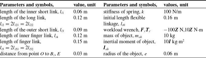
Table I lists the parameters of the hybrid hand. Based on the theoretical formula in Section 2–5, a program is written using MATLAB/Maple. The kinematics theoretical solutions of the hybrid hand are solved, see Figure 5. When grabbing heavy objects, the gravity of each link of the hybrid hand can be ignored in the dynamics calculation. When the radius of the grasped object is e = 0.06 m, and the spring is not deformed, when d_i = 0.113 m, each fingertip of the hybrid hand contacts the surface of the object, let the grasping posture as the initial grasping posture. When the initial force of the spring F _si0 = 0 (i = 1,2,3), the values change of v_di (i = 1,2,3) and a_di (i = 1,2,3) as shown in Figure 5c and e, solving the kinematic theoretical solutions of the grasping object by the hybrid hand, see Figure 6a-f. Let η = 1, the dynamics theoretical solutions of driving forces f_ai (i = 1,2,3), constrained forces f_cj (j = 1,2,3) and spring forces F_si (i = 1,2,3) of the hybrid hand are solved, see Figure 6g-i.

Table I.

Parameters of the hybrid hand.

Figure 6.

Theoretical kinematics and dynamics solutions of the hybrid hand grasping object.

Figure 7.

A simulation mechanism of hybrid hand mechanism. (a) A main block model of simulation mechanism. (b) Finger 1 subsystem.

Based on the changes in the movement and force parameters of the hybrid hand during each grasping process, as illustrated in Figure 5 and Figure 6, the following conclusions can be drawn:

With the change of the driving position, the grasping pose of the hybrid hand changes steadily, proving that the DOF of the hybrid hand is consistent with the calculation results. In the case of the contact points and the shape of the object are determined, the hybrid hand can grasp the object without the need for complex control algorithms. During the grasping process, there is a smooth transition in both motion and force parameters. Simultaneously, the force F_si (i = 1,2,3) act on the spring in each flexible rod increases steadily. This indicates that the spring serves as a flexible protective mechanism for the object being grasped. The curve representing this change is gradual, with no abrupt fluctuations in force, demonstrating that the hybrid hand possesses the capability for compliant grasping.

According to the change of the drive displacement d_i (i = 1,2,3), the grasping posture of the hybrid hand gradually becomes tighter, unlike the traditional robot hand, the values of the drive force and the constraint force of the hybrid hand are not both increasing, which indicates that by controlling the posture of the hybrid hand, the hybrid hand can make the grip tighter while decreasing the drive force.

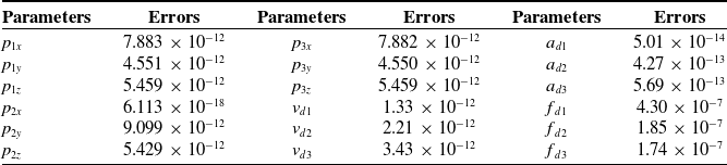
To verify the theoretical solutions of the hybrid hand, a high-precision simulation model is essential. Various disturbances occur during the movement of the experimental prototype, including frictional forces and gaps present in the joints, which significantly impact the experimental results. These errors can be avoided through settings in the simulation model. Additionally, during the grasping of the experimental prototype, many parameters, such as constrained force and spring force, are difficult to observe directly. The simulation mechanism of the hybrid hand in MATLAB/Simulink/Mechanics is constructed, see Figure 7. The absolute errors between the maximum value x of the theoretical solution and the maximum value xs of the simulation solution are given in Table II. It is known from Table II that the theoretical solutions of the kinematics and dynamics models coincide with that of the simulation mechanism.

Table II.

Absolute errors between the theoretical solutions and the simulation solutions (unit: m, m/s, N).

As shown in Figure 8, the hybrid hand is capable of grasping objects of various sizes and materials without requiring complex control methods, even for delicate items such as eggs. The grasp load of the hybrid hand mechanism prototype is measured by the force sensor and displayed by computer software, which can display the force change of eight sensors in real-time, and its control and measurement system is shown in Figure 9. By utilizing the movement of the auxiliary mechanical arm, the hybrid hand can reach the target position and grasp the object. The sensor measurement software is capable of measuring the force values of the sensors in real time.

Figure 8.

Hybrid hands grasp objects of various shapes and materials. (a) A box is grasped. (b) An egg is grasped. (c) An apple is grasped. (d) A cylinder cup is grasped. (e) 2 kg weight is grasped. (f) 4 kg weight is grasped.

Figure 9.

Hybrid hand grasp and measurement experiment.

As illustrated in Figure 8 e-f, the hybrid hand grasped the weights at different bending degrees, and the measurement results of the sensor force f_i (i = 1,2,3) on the fingertip were shown in Figure 10. In Figure 10 a, the hybrid hand is used to grasp a 0.5 kg object. The number of 0.5 kg objects is increased to increase the load, as shown in Figure 8 e. In Figure 10 b, a 2 kg object is grasped by the hybrid hand, and the number of 0.5 kg weights is increased to increase the load.

Figure 10.

Measured results of sensor forces f_i(i = 1,2,3) of three fingertips for grasping object.

The grasping experiment and measurement results of the hybrid hand show that:

1. 1. The hybrid hand has good adaptive and flexible grasping ability, safely grasping objects of various shapes and materials without complex control algorithms.

2. 2. The maximum diameter of the grasp of the hybrid hand prototype is 265 mm, and all fingertips can reach a point to ensure that the hybrid hand can grasp small objects, indicating that the hybrid hand has a large workspace.

3. 3. The hybrid hand can grasp heavy objects, the hybrid hand has two ways of grasping objects, including fingertip grasping or envelope grasping.

4. 4. The force sensor in the fingertip of the hybrid hand can be used to measure the weight of the grasped object and the value of the contact force, and the sensor is not easy to wear. When utilizing a hybrid hand to grasp objects of varying masses, the mass of the grasped object is approximately directly proportional to the sensor measurement values. Therefore, by using the average measurement values from each finger sensor as a reference for the hybrid hand’s grasp, the mass of the object can be estimated. However, since the contact points and grasping poses can influence the force readings of each finger sensor, it is essential to maintain consistency in the positions of each contact point and the grasping posture. Additionally, errors can be minimized by enhancing the precision of the components.

The method for estimating the mass of an object is as follows: Let M_c be the calibration value for the hybrid hand grasping, let M_u be the actual value of the unknown object, and let M_us be the measured and calculated value of the unknown object, and let K be the calibration ratio, which can be calculated by $K=\sum f_{ic}/\sum f_{iu}=M_{c}/M_{us}$ . During the grasping of an object, the approximate mass M_us of the grasped object can be evaluated using the equation M_us=M _c/K. Let Δ _M be the relative error between M_u and M_us, and Δ _M can be calculated by $\Delta _{M}=\mathrm{abs}(M_{u}-M_{us})/M_{u}\times 100\boldsymbol{\% }$ . For example, two sets of data can be taken from each of Figure 10 a-b, representing different mass ranges of the grasped objects, to verify the effectiveness of this method. When M={(1,1.5), (3, 3.5)}kg is taken, the corresponding of {f_i (i = 1,2,3)} are taken as the calibration values {f_ic (i = 1,2,3)} and the measured values {f_iu (i = 1,2,3)} respectively. The calculated mass M_us is compared with the actual mass M_u to analyze the accuracy of the measurement, as shown in Table III. According to the final comparison results, it can be concluded that after the hybrid hand is calibrated by grasping a standard object, the mass of the grasped object can be estimated using the sensor measurement values.

Table III.

Approximate mass M_u of grabbed object and its error.