1. Introduction
Through long-term natural selection, flying and swimming animals that use oscillatory propulsion have evolved the ability to move with remarkably high efficiency. A critical dimensionless parameter that links propulsive performance to kinematics of tails and wings is the Strouhal number (
 $St$
), defined as the product of oscillatory frequency and stroke amplitude divided by the moving speed. Observational data indicate that fish and cetaceans typically achieve the optimum propulsion within a narrow
 $St$
range of 0.25–0.35 (Triantafyllou et al. Reference Triantafyllou1991, Reference Triantafyllou, Triantafyllou and Grosenbaugh1993, Reference Triantafyllou, Triantafyllou and Yue2000). Further investigations by Rohr & Fish (Reference Rohr and Fish2004), examining the locomotion of seven species of odontocete cetaceans over a broad range of forward speeds, confirmed that most cetaceans prefer swimming at
 $St$
values between 0.20 and 0.40. Similarly, Eloy (Reference Eloy2012) conducted a comprehensive analysis of the swimming kinematics of 53 species of aquatic animals, reporting an analogous optimal range for
 $St$
in oscillatory-based swimmers. Despite variations in swimming speed and body size, the optimal
 $St$
range of
 $0.20 \lt St \lt 0.40$
is conserved across different Reynolds numbers according to these observations. More interestingly, Nudds et al. (Reference Nudds, John, Keen and Shiels2014) found that fish can maintain their preferred
 $St$
values through a trade-off between tail beat frequency and peak-to-peak stroke amplitude, even when water temperature changes, suggesting a consistent occurrence of optimal
 $St$
in fish swimming. By analogy, Taylor et al. (Reference Taylor, Nudds and Thomas2003) analysed the Strouhal numbers of 42 species of birds, bats and insects, discovering that the optimal
 $St$
range for flying animals also converges within the interval of 0.20–0.40. Thus, optimising Strouhal numbers into this constrained range by tuning swimming and flying kinematics appears to be a general principle for animals employing oscillatory propulsion to achieve efficient cruising. In addition, Gazzola et al. (Reference Gazzola, Argentina and Mahadevan2014) examined the existing locomotion data spanning a large number of aquatic swimmers and discovered the same converging behaviour of Strouhal number as the above findings. Especially, they derived a scaling relation that links cruising speed to body kinematics and fluid properties, which provides a physical basis for the observations that swimming and flying animals commonly operate within a narrow
 $St$
range.
The growing interest in efficient cruising of animals has inspired the development of innovative propulsion systems for both autonomous underwater vehicles and micro air vehicles. An oscillating foil, undergoing combined heaving and pitching motion with a specific phase difference, serves as an effective analogy to natural oscillatory fins and wings. Anderson et al. (Reference Anderson, Streitlien, Barrett and Triantafyllou1998) and Read et al. (Reference Read, Hover and Triantafyllou2003) conducted a number of experimental measurements on the propulsive performance of an isolated oscillating foil, and found that significantly high efficiency can be attained by an appropriate combination of kinematic and geometric parameters. Notably, they indicated that the efficiency of a harmonically heaving and pitching foil tends to peak within the
 $St$
range of 0.20–0.40, consistent with biological observations. Inspired by the pectoral fins of aquatic animals, Techet (Reference Techet2008) experimentally measured the propulsive performance of a three-dimensional rolling and pitching foil at high Reynolds numbers. He also observed the optimum efficiency within the interval
 $0.20 \lt St \lt 0.40$
, with a maximum efficiency at
 $St = 0.30$
. Using an idealised model of an elliptical foil subjected to vertical oscillation, Deng & Caulfield (Reference Deng and Caulfield2016, Reference Deng and Caulfield2018) observed that the foil transitions into a self-propelled state, achieving nearly constant horizontal speeds after symmetry breaking occurs. The resulting Strouhal numbers fall within the range of 0.32–0.40 for two-dimensional cases and 0.25–0.35 for three-dimensional cases (oblate spheroids) when the aspect ratio is less than 0.4. Floryan et al. (Reference Floryan, Van Buren, Rowley and Smits2017) and Van Buren et al. (Reference Van Buren, Floryan and Smits2019) employed the comprehensive propulsive data to propose new scaling laws for thrust, power and efficiency of oscillating foils. When plotted as a function of Strouhal number, the maximum efficiency tends to converge on the optimal range
 $0.20 \lt St \lt 0.40$
, whether for purely heaving/pitching foils or oscillating foils in combined heaving and pitching motion. These findings are further supported by extensive theoretical analyses and numerical simulations (Guglielmini & Blondeaux Reference Guglielmini and Blondeaux2004; Young & Lai Reference Young and Lai2007; Lua et al. Reference Lua, Dash, Lim and Yeo2016; Şentürk & Smits Reference Şentürk and Smits2019), indicating that the Strouhal number must be tightly constrained to achieve efficient propulsion.
The following question then arises. Why does optimum efficiency consistently occur within the range of
 $0.20 \lt St \lt 0.40$
for both biological appendages and artificial foils? A stability analysis by Triantafyllou et al. (Reference Triantafyllou1991, Reference Triantafyllou, Triantafyllou and Grosenbaugh1993) indicated that the average velocity profile in the wake of an oscillating foil exhibits a jet pattern, which becomes convectively unstable over a narrow range of frequencies corresponding to this optimal
 $St$
interval. They proposed that optimum efficiency is achieved within this specific Strouhal number range because the oscillatory frequency of the foils coincides with the frequency of maximum spatial amplification of disturbances. From an aerodynamic or hydrodynamic perspective, the viscous effects play a significant role and thus the drag dominates the streamwise force when foils perform weak motion at low Strouhal numbers, resulting in poor efficiency (Smits Reference Smits2019). As the Strouhal number increases, the influence of drag force becomes weaker. Established scaling laws for the propulsive performance of oscillating foils, derived from circulatory and added mass forces, indicate that both the thrust production and power expenditure increase nonlinearly with
 $St$
, leading to a rapid rise in efficiency to a peak at a specific
 $St$
value, followed by a mild decline (Floryan et al. Reference Floryan, Van Buren, Rowley and Smits2017; Van Buren et al. Reference Van Buren, Floryan and Smits2019). Given that the maximum angle of attack is determined by the Strouhal number, a strong foil motion at extremely high
 $St$
may induce large-scale flow separation and dynamic stall behaviours, significantly reducing propulsive efficiency (Isogai et al. Reference Isogai, Shinmoto and Watanabe1999; Tuncer & Kaya Reference Tuncer and Kaya2005; Young & Lai Reference Young and Lai2007). Additionally, the optimal frequency of oscillating foils was thought to be selected by intrinsic time scales associated with vortex growth and leading-edge vortex shedding (Wang Reference Wang2000), suggesting that the Strouhal numbers are inherently related to propulsive performance.
Owing to tremendous efforts, the understandings of oscillatory swimming and newly developed propulsion systems inspired by natural swimmers have reached an encouraging level (Rozhdestvensky & Ryzhov Reference Rozhdestvensky and Ryzhov2003; Platzer et al. Reference Platzer, Jones, Young and Lai2008; Wu Reference Wu2011; Smits Reference Smits2019). The literature in this field spans a broad range of aspects, including performance optimisation (Tuncer & Kaya Reference Tuncer and Kaya2005; Izraelevitz & Triantafyllou Reference Izraelevitz and Triantafyllou2014), the roles of flexibility (Zhu Reference Zhu2007; Alben Reference Alben2008), flow structure manipulation (Liao et al. Reference Liao, Beal, Lauder and Triantafyllou2003; Fish & Lauder Reference Fish and Lauder2006), three-dimensional effects (Dong et al. Reference Dong, Mittal and Najjar2006; Buchholz & Smits Reference Buchholz and Smits2008) and the characteristics of multi-foil arrangements (Muscutt et al. Reference Muscutt, Weymouth and Ganapathisubramani2017; Alben Reference Alben2021). However, existing studies on oscillatory propulsion have mostly focused on homogeneous environments. In reality, oceans are inherently stratified in density due to variations in temperature, salinity and pressure with depth (Thorpe Reference Thorpe2005). Especially for the upper layer of the ocean where the density gradient is notably high, known as pycnocline, stratification effects play an important role in the locomotion and hydrodynamics of swimmers (More & Ardekani Reference More and Ardekani2023). Despite the oceanic density gradient covering a large spatial scale, the fundamental length scale that dictates stratification effects on the motion of marine swimmers was found to be much smaller and comparable with that of biological activity (Ardekani & Stocker Reference Ardekani and Stocker2010). The significant role of density stratification has been identified in many physical processes, ranging from wake evolution of metre-scale objects (Spedding Reference Spedding2014) to settling dynamics of centimetre-scale zooplankton (Magnaudet & Mercier Reference Magnaudet and Mercier2020). It is therefore anticipated that either natural oscillatory swimmers, such as fish and mammals (Gazzola et al. Reference Gazzola, Argentina and Mahadevan2014), or man-made devices, such as underwater vehicles and gliders equipped with oscillating wings (Zhou & Low Reference Zhou and Low2011; Rozhdestvensky Reference Rozhdestvensky2022), will exhibit distinct dynamical behaviours in stratified environments with a sufficiently large density gradient when compared with homogeneous observations. This raises the following crucial question. What are the preferred Strouhal numbers for oscillatory propulsion in a density stratified fluid? Our study aims to address this question.
Fluid parcels displaced vertically in a stratified environment experience a buoyancy-driven restoring force, leading to distinctive phenomena that challenge the mechanisms and principles established in homogeneous fluids. The literature on the interaction between density stratification and structures covers a wide range of topics. One of the most prominent features in a stably stratified fluid is the triggering of internal waves, which plays a crucial role in mass and momentum transport in oceans (Sutherland Reference Sutherland2010). Early studies primarily focused on modelling and measuring internal wave dynamics (Hurley & Keady Reference Hurley and Keady1997; Flynn et al. Reference Flynn, Onu and Sutherland2003), significantly advancing our understanding of their generation and propagation mechanisms. More recent research has increasingly focused on nonlinear effects, such as wave–flow interactions, wave breaking events and energy transfer (Allshouse et al. Reference Allshouse, Lee, Morrison and Swinney2016; Howland et al. Reference Howland, Taylor and Caulfield2021). In addition, wake dynamics of bodies with varying shapes in stratified fluids have garnered significant attention. Early efforts can be traced back to the studies on the evolution of vortices generated by either two- or three-dimensional wings in a stratified fluid (Sarpkaya Reference Sarpkaya1983; Spalart Reference Spalart1996). By revealing the leading mechanisms governing the rise, demise and trajectory of the vortices, these works enhance the comprehension into the interaction of aircraft wakes and stratified atmospheres, and thus offer important implications for air traffic control. For bluff bodies in horizontal motion, the wakes are characterised by the persistence of coherent structures with a high horizontal–vertical length ratio due to the inhibition of vertical motion (Spedding et al. Reference Spedding, Browand and Fincham1996; Meunier & Spedding Reference Meunier and Spedding2006). Madison et al. (Reference Madison, Xiang and Spedding2022) further indicated that the wake structures of a body towed at a constant horizontal speed can be categorised into different flow regimes, depending on the relative contributions of inertial, buoyancy and viscous effects. In the case of a sphere moving vertically at a constant speed, the flow pattern was shown to exhibit a strong rear jet due to the complete collapse of the axisymmetric standing vortex under stratification effects (Torres et al. Reference Torres, Hanzaki, Ochoa, Castillo and Van Woert2000; Okino et al. Reference Okino, Akiyama and Hanazaki2017).
Considerable research has also been devoted to the dynamics of freely moving bodies in a stratified fluid. Doostmohammadi et al. (Reference Doostmohammadi, Dabiri and Ardekani2014) reported that the settling dynamics of a sphere can be influenced significantly by the presence of stratification. They observed an oscillation in settling velocity and even levitation behaviour after the sphere reaches peak speed. Lam et al. (Reference Lam, Vincent and Kanso2019) examined the fluttering behaviour of rigid discs falling freely in stably stratified fluids, and found that density stratification tends to increase radial dispersion while greatly reducing peak inclination angle, fluttering amplitude and vertical descent velocity. More & Ardekani (Reference More and Ardekani2020) investigated the influence of density stratification on the self-propulsion characteristics of a squirmer, noting that a pusher propelling from the rear is a more efficient swimmer than a puller propelling from the front due to more efficient advection of vorticity downstream. These studies provide valuable insights into the contribution of swimming organisms and sedimenting particles to the mixing process in oceans and lakes (Ardekani et al. Reference Ardekani, Doostmohammadi and Desai2017; Houghton et al. Reference Houghton, Koseff, Monismith and Dabiri2018).
In contrast to the extensive research on stratification-induced alteration of flow structures, relatively few studies have focused on the hydrodynamic forces acting on submersed bodies in stratified fluids. Lofquist & Purtell (Reference Lofquist and Purtell1984) and Arntsen (Reference Arntsen1996) examined the drag force of bluff bodies moving horizontally in stably stratified fluids and reported an evident sensitivity of the drag coefficient to the strength of stratification. Additionally, Ermanyuk & Gavrilov (Reference Ermanyuk and Gavrilov2002, Reference Ermanyuk and Gavrilov2003) explored the hydrodynamic loads on both two-dimensional circular cylinders and three-dimensional spheres oscillating horizontally under stratification conditions, revealing a clear dependence of added mass and damping coefficients on the vertical extent of stratification. These findings suggest that the force characteristics of bodies in stratified fluids differ both qualitatively and quantitatively from those in homogeneous fluids. Nonetheless, the physical mechanisms underlying such differences in force and moment, particularly for swimmers with a complex motion mode, remain inadequately understood.
Our previous study (Wang et al. Reference Wang, Kandel and Deng2024) has evaluated the hydrodynamic performance of a combined heaving and pitching foil at a constant Strouhal number, finding that both thrust production and propulsive efficiency are enhanced through the proper resonance between foil kinematics and stratification effects. Building on the knowledge that the highest efficiency of oscillatory propulsion consistently occurs within a narrow
 $St$
interval in homogeneous fluids, we conduct new numerical simulations to examine the optimal Strouhal numbers for an oscillating foil in a density stratified fluid. This study seeks to provide new insights into the role of density stratification in optimising Strouhal numbers of oscillatory propulsion and offer novel information for flow patterns generated by oscillating bodies in stratified regimes.
2. Methodology
2.1. Problem formulation and governing parameters
We consider a two-dimensional NACA0012 aerofoil undergoing combined heaving
 $h(t)$
and pitching
 $\theta (t)$
motion in a uniform inflow with a constant velocity
 $U_\infty$
(see figure 1
 $a$
). The aerofoil rotates about a pivot point with a distance
 $b$
from the leading edge. The foil’s motion is described by
 \begin{equation} h(t) = {h_0}\sin (2\pi ft), \quad \theta (t) = {\theta _0}\sin (2\pi ft + \phi ), \end{equation}
where
 $f$
is the oscillation frequency,
 $h_0$
is the heave amplitude,
 $\theta _0$
is the pitch amplitude, and
 $\phi$
is the phase difference between heave and pitch. As illustrated in figure 1(
 $b$
), the instantaneous angle of attack
 $\alpha (t)$
is given by
 \begin{equation} \alpha (t) = \arctan \left(\frac {1}{{{U_\infty }}}\frac {{\mathrm {d}h(t)}}{{\mathrm {d}t}}\right) - \theta (t). \end{equation}
When the pitch leads the heave by
 $\phi = 90^\circ$
, the maximum angle of attack
 $\alpha _0$
can be obtained by
 \begin{equation} {\alpha _0} = \arctan \left(\frac {{2\pi {h_0}f}}{{{U_\infty }}}\right) - {\theta _0}. \end{equation}
The choice of aerofoil geometry and inflow velocity in our simulations follows the set-ups of the experiments by Anderson et al. (Reference Anderson, Streitlien, Barrett and Triantafyllou1998) and Read et al. (Reference Read, Hover and Triantafyllou2003), ensuring that the involved parameters are relevant to biological propulsion in nature.
(a) Schematic of the computational domain with a size of
 $100c \times 100c$
. The initial background density is set as a linear profile:
 ${\rho _b}(y) = {\rho _0} - \gamma y$
, with a constant density gradient
 $\gamma$
along the
 $y$
direction. Note that foil size is exaggerated for better visibility. (b) Illustration of the foil kinematics, where the foil performs combined heaving
 $h(t)$
and pitching
 $\theta (t)$
motion in a uniform inflow with a constant velocity
 $U_\infty$
, leading to an instantaneous angle of attack
 $\alpha (t)$
.

For a foil that simultaneously heaves and pitches in density stratified fluids, three dimensionless parameters govern the problem: the chord-based Reynolds number
 $Re$
, the amplitude-based Strouhal number
 $St$
and the internal Froude number
 $Fr$
:
 \begin{equation} Re = \frac {{{U_\infty }c}}{\nu }, \quad St = \frac {{2{h_0}f}}{{{U_\infty }}}, \quad Fr = \frac {{{U_\infty }}}{{ND}}, \end{equation}
where
 $\nu$
is the kinematic viscosity,
 $D$
is the maximum thickness of the foil and
 $N$
is the Brunt–Väisälä frequency signifying the natural oscillation frequency of fluid particles in a stratified fluid. The above expression for
 $St$
is based on the approximation that the characteristic width of the wake is equivalent to the lateral total excursion of the foil (Triantafyllou et al. Reference Triantafyllou, Triantafyllou and Yue2000). We consider a linearly stratified fluid with a constant density gradient
 $\gamma$
in the direction of gravitational acceleration
 $\boldsymbol {g}$
. The background density profile is set as
 ${\rho _b}(y) = {\rho _0} - \gamma y$
(see figure 1
 $a$
), where
 $\rho _0$
is the reference fluid density and
 $y$
is the vertical coordinate. The Brunt–Väisälä frequency is given by
 $N = {(\gamma g/{\rho _0})^{1/2}}$
. We select the value of
 $\gamma$
to ensure that the maximum density variation does not exceed 5 % of
 $\rho _0$
, thereby satisfying the Boussinesq approximation for stratified fluids. When executing a fully prescribed motion, the oscillating foil is assumed to maintain a neutrally buoyant state. Therefore, the desired
 $Fr$
can be easily achieved by adjusting
 $g$
in our simulations.
The primary parameters in this study are selected as
 ${h_0}/c = 0.75$
,
 $\phi = 90^\circ$
,
 ${\alpha _0} = 15^\circ$
and
 $b/c = 1/3$
. These values are chosen based on previous studies indicating that such parameter settings tend to yield satisfactory propulsive performance for oscillating foils in homogeneous fluids (Anderson et al. Reference Anderson, Streitlien, Barrett and Triantafyllou1998; Read et al. Reference Read, Hover and Triantafyllou2003). However, whether this combination of parameters represents an optimal choice for stratified fluids remains an open question. The frequency
 $f$
is adjusted to achieve the desired
 $St$
and the constant
 $\alpha _0$
is attained by varying
 $\theta _0$
. The Reynolds number is fixed at
 $Re = 1000$
for all simulations. This relatively low-turbulence regime has been widely studied in the context of hydrodynamic performance and wake evolution of oscillating foils (Anderson et al. Reference Anderson, Streitlien, Barrett and Triantafyllou1998; Godoy-Diana et al. Reference Godoy-Diana, Aider and Wesfreid2008; Verma & Hemmati Reference Verma and Hemmati2022), suggesting that Reynolds numbers of the order of
 $O({10^3})$
are sufficient to capture key features of oscillating-based propulsion. Moreover, Gazzola et al. (Reference Gazzola, Argentina and Mahadevan2014) performed a comprehensive analysis on biological measurements and found that the preferred Strouhal number of swimming animals stabilises once the Reynolds number, based on body length, exceeds a critical value. In our simulations, the chord-length Reynolds number corresponds to a body-length Reynolds number within a flow regime where the Reynolds number has minimal effect on the Strouhal number (Gazzola et al. Reference Gazzola, Argentina and Mahadevan2014).
Our central focus is on the parameter space defined by
 $St$
, characterising the foil kinematics, and
 $Fr$
, characterising the stratification strength. The
 $St$
and
 $Fr$
are varied within the ranges of
 $0.1 \leqslant St \leqslant 0.6$
, with an interval
 $\Delta St = 0.05$
, and
 $1 \leqslant Fr \leqslant 10$
, with an interval
 $\Delta Fr = 0.5$
. This
 $St$
range covers the majority of Strouhal numbers observed in natural swimmers and examined in the studies of oscillating foils. The
 $Fr$
range considered here encompasses a spectrum of stratification strengths from strong to weak. Given typical
 $N$
values in real stratified environments (Thorpe Reference Thorpe2005), the internal Froude numbers for biological appendages or artificial foils with a length scale of
 $O$
(1m) can fall within the considered
 $Fr$
range when cruising at feasible speeds.
A combined heaving and pitching foil experiences instantaneous streamwise force
 ${F_x}(t)$
, transverse force
 ${F_y}(t)$
and torque
 $Q(t)$
about the rotation axis. The time-averaged thrust production and input power over one oscillation cycle
 $T$
are calculated by
 \begin{align} \bar F = \frac {1}{T}\int _0^T {{F_x}(t)\mathrm {d}t}, \qquad\qquad\qquad\end{align}
 \begin{align} \bar P = \frac {1}{T}\left ( {\int _0^T {{F_y}(t)\frac {{\mathrm {d}h(t)}}{{\mathrm {d}t}}\mathrm {d}t + \int _0^T {Q(t)\frac {{\mathrm {d}\theta (t)}}{{\mathrm {d}t}}\mathrm {d}t} } } \right ). \end{align}
The performance metrics of an oscillating foil are characterised by the time-averaged thrust coefficient
 $C_T$
, power coefficient
 $C_P$
and propulsive efficiency
 $\eta$
:
 \begin{equation} {C_T} = \frac {{\bar F}}{{0.5{\rho _0}U_\infty ^2cs}}, \quad {C_P} = \frac {{\bar P}}{{0.5{\rho _0}U_\infty ^3cs}}, \quad \eta = \frac {{\bar F{U_\infty }}}{{\bar P}} = \frac {{{C_T}}}{{{C_P}}}, \end{equation}
where
 $s$
denotes the foil span, taking as unit length in two-dimensional cases. Each simulation is run for eight oscillation cycles, with time-averaged results computed from the final cycle. Our findings indicate that the system reaches a periodic state by the fourth oscillation cycle. In this study, both instantaneous and time-averaged force metrics are normalised using the free stream velocity as the velocity scale and the aerofoil chord length as the length scale, following the conventions established in studies of oscillatory propulsion. This normalisation allows for direct comparison of the propulsive characteristics between the present stratified fluid results and relevant homogeneous observations in the literature. It is noteworthy that recent experiments and theories suggest more appropriate scales for hydrodynamic performance of oscillating foils (Smits Reference Smits2019). One can refer to newly proposed scaling laws for more details (Floryan et al. Reference Floryan, Van Buren, Rowley and Smits2017; Van Buren et al. Reference Van Buren, Floryan and Smits2019).
2.2. Numerical methods
The two-dimensional incompressible stratified flow around an oscillating foil is simulated using a finite-volume solver. The fluid motion is governed by the conservation equations of mass, momentum and density under the Boussinesq approximation, assuming that the density variations appear only in the buoyancy force term and are negligible compared with the reference density. The density
 $\rho$
and pressure
 $p$
fields are split into background and fluctuating components, expressed as
 $\rho = {\rho _b} + \rho '$
and
 $p = {p_b} + p'$
. The background density
 $\rho _b$
follows a linear profile, as previously specified. The background pressure
 $p_b$
satisfies the hydrostatic balance
 $\boldsymbol {\nabla } {p_b} = {\rho _b}\boldsymbol {g}$
. The fluctuating quantities,
 $\rho '$
and
 $p'$
, arise from the fluid motion. The governing equations are therefore given by
 \begin{align} \boldsymbol {\nabla } \boldsymbol {\cdot } \boldsymbol{u} = 0, \qquad\qquad\qquad\qquad\end{align}
 \begin{align} \frac {{\partial \boldsymbol{u}}}{{\partial t}} + \boldsymbol{u} \boldsymbol {\cdot } \boldsymbol {\nabla } \boldsymbol{u} = - \frac {1}{{{\rho _0}}}\boldsymbol {\nabla } p' + \nu {\nabla ^2}\boldsymbol{u} + \frac {{\rho '}}{{{\rho _0}}} \boldsymbol {g}, \,\,\end{align}
 \begin{align} \frac {{\partial \rho '}}{{\partial t}} + \boldsymbol{u} \boldsymbol {\cdot } \boldsymbol {\nabla } \rho ' + \boldsymbol{u} \boldsymbol {\cdot } \boldsymbol {\nabla } {\rho _b} = \frac {\nu }{{Pr}}{\nabla ^2}({\rho _b} + \rho '), \end{align}
where
 $\boldsymbol{u}$
is the fluid velocity,
 $t$
denotes time and
 $Pr$
is the Prandtl number, representing the ratio of momentum to thermal diffusivity. Given that temperature variation is the primary factor influencing density changes in aquatic environments (Sutherland Reference Sutherland2010), we set the Prandtl number to
 $Pr = 7$
, a typical value for thermally stratified fluids. In our numerical simulations, the grid spacing near the foil surface is carefully designed to resolve both the momentum and density boundary layers for the Reynolds and Prandtl numbers considered. According to Schlichting & Gersten (Reference Schlichting and Gersten2016), the boundary-layer thicknesses for momentum and density can be estimated as
 ${\delta _m} \sim O(D/\sqrt {Re} )$
and
 ${\delta _d} \sim O(D/\sqrt {RePr} )$
, respectively.
The configuration of the computational domain is illustrated in figure 1(
 $a$
). We use an arbitrary Lagrangian–Eulerian formulation to solve the governing equations on a moving grid, which comprises two zones interconnected through a circular sliding interface. The inner circular zone, with a radius of
 $10c$
, undergoes rigid rotation to account for the foil pitch, while grid deformation in the outer zone implements the foil heave. To prevent spurious reflection of internal waves, our numerical model employs a significantly large domain size (
 $100c \times 100c$
) with considerable distances between the foil and boundaries.
The solver uses the first-order implicit Euler scheme to advance the equations in time. The spatial derivatives of convection and diffusion terms are discretised using second-order upwind and central-difference schemes, respectively. The pressure–velocity coupling is resolved using the pressure implicit with splitting of operators (PISO) algorithm. We set the boundary condition of the oscillating foil as a moving wall with no flux normal to the surface. A uniform constant velocity is imposed at the inlet boundary, while the outlet boundary employs a convective outflow condition. The pressure field is treated with a Dirichlet boundary condition at the top and a Neumann boundary condition at the other boundaries. A Neumann boundary condition is applied at all boundaries for the density field.
It is noteworthy that the momentum equation employed in our previous study (Wang et al. Reference Wang, Kandel and Deng2024) is
 \begin{equation} \frac {{\partial \boldsymbol{u}}}{{\partial t}} + \boldsymbol{u} \boldsymbol {\cdot } \boldsymbol {\nabla } \boldsymbol{u} = - \frac {1}{{{\rho _0}}}\boldsymbol {\nabla } p'' + \nu {\nabla ^2}\boldsymbol{u} - \frac {{\boldsymbol {g} \boldsymbol {\cdot } \boldsymbol {r}}}{{{\rho _0}}}\boldsymbol {\nabla } \rho , \end{equation}
where
 $\boldsymbol {r} = (x, y, z)$
is the position vector and
 $p''$
represents the flow-induced pressure. Both (2.11) and (2.9) are derived from the standard incompressible momentum equation based on the Boussinesq approximation. They are mathematically equivalent with the only difference in the form of the flow-induced pressure. From a computational standpoint, solving the density perturbation directly (the last term on the right-hand side of (2.9)) is found to double the computational time compared with solving the gradient of density perturbation (the last term on the right-hand side of (2.11)). That is why (2.11) was used in our previous study (Wang et al. Reference Wang, Kandel and Deng2024). By solving (2.11), we have
 $p = p'' + \rho \boldsymbol {g} \boldsymbol {\cdot } \boldsymbol {r}$
, where
 $\rho \boldsymbol {g} \boldsymbol {\cdot } \boldsymbol {r}$
approximates the hydrostatic pressure component, as
 $\rho '$
is insignificant compared with
 $\rho _0$
. However, our recent computations indicate that despite
 $\rho ' \ll {\rho _0}$
, the approximation of
 ${p_b} = \rho \boldsymbol {g} \boldsymbol {\cdot } \boldsymbol {r}$
leads to an overestimate in the thrust production of oscillating foils.
In the current study, we solve (2.9) to obtain the flow-induced pressure
 $p'$
. This approach yields
 $p = p' + 0.5({\rho _0} + {\rho _b})\boldsymbol {g} \boldsymbol {\cdot } \boldsymbol {r}$
, where the hydrostatic pressure component
 ${p_b} = 0.5({\rho _0} + {\rho _b})\boldsymbol {g} \boldsymbol {\cdot } \boldsymbol {r}$
is calculated through the hydrostatic balance
 $\boldsymbol {\nabla } {p_b} = {\rho _b}\boldsymbol {g}$
, along with the linear background density
 ${\rho _b}(y) = {\rho _0} - \gamma y$
. The hydrostatic pressure component can be rearranged as
 ${p_b} = - {\rho _0}gy + 0.5g\gamma {y^2}$
, consistent with Ardekani & Stocker (Reference Ardekani and Stocker2010). This update is believed to provide more accurate predictions for the hydrodynamic performance of an oscillating foil in stratified fluids. The correction of the hydrostatic pressure is the primary cause of the discrepancies between the results presented in this study and those reported in our previous work (Wang et al. Reference Wang, Kandel and Deng2024). Additionally, the Prandtl number was set to
 $Pr = 1$
in our previous simulations (Wang et al. Reference Wang, Kandel and Deng2024), which accounts for a discrepancy less than
 $10\,\%$
.
The numerical solver used in this study has been extensively validated and successfully applied to various problems involving stratified fluids (Deng & Kandel Reference Deng and Kandel2022; Kandel & Deng Reference Kandel and Deng2022; Wang et al. Reference Wang, Deng, Kandel and Sun2023a
,Reference Wang, Wang and Deng
b
). In the Appendix, a sensitivity analysis is performed concerning grid resolution, time step and computational domain size for the most challenging case
 $(St = 0.6, Fr =1)$
within the parameter space considered here.
3. Parametric studies on propulsive performance
We carry out a parametric study by scanning the
 $(St, Fr)$
parameter space, which covers the ranges of
 $0.1 \leqslant St \leqslant 0.6$
and
 $1 \leqslant Fr \leqslant 10$
. Our focus is on identifying the optimal Strouhal numbers
 $S{t_m}$
for oscillatory propulsion in stratified fluids. We first present primary observations here and then elucidate underlying mechanisms driving these behaviours in the subsequent sections. We limit the discussion of the foil’s optimal kinematic conditions to the Strouhal number alone. Given that the propulsive performance of an oscillating foil is influenced by a wide range of kinematic and geometric parameters, it is expected that altering the parameters held constant in our simulations could also yield high thrust production and efficiency in stratified fluids, similar to the effects achieved by tuning the Strouhal number. This may lead to the identification of other optimal conditions, which remains an open question for future research.
Contour plots of time-averaged (a) thrust coefficient
 $C_T$
and (b) power coefficient
 $C_P$
over one oscillation cycle for an oscillating foil in the
 $(St, Fr)$
parameter space.

Figure 2 displays the contour plots for time-averaged thrust and power coefficients. The oscillating foil initially generates drag at very low
 $St$
, which transitions to thrust as
 $St$
increases. Both thrust and power under the stratification influence increase monotonically with
 $St$
, aligning with the observations in homogeneous fluids. However, the rate of change of
 $C_T$
and
 $C_P$
with
 $St$
depends on the Froude number. Significant variations in thrust and power are observed at low
 $Fr$
, resulting in high-intensity regimes in the lower-right corner of the
 $(St, Fr)$
plane. The monotonic variation of time-averaged metrics in figure 2 indicates that
 $C_T$
and
 $C_P$
can be scaled with a combination of
 $St$
and
 $Fr$
. Inspired by extensive efforts to scale oscillatory propulsion in homogeneous fluids (Quinn et al. Reference Quinn, Moored, Dewey and Smits2014; Floryan et al. Reference Floryan, Van Buren, Rowley and Smits2017; Van Buren et al. Reference Van Buren, Floryan and Smits2019) and the scaling laws derived by Zhang et al. (Reference Zhang, Mercier and Magnaudet2019) for the drag on a settling body in stratified fluids, we propose a simplified scaling relation to characterise the numerical data presented in this study:
 \begin{equation} {C_T} = {c_1}S{t^{{\alpha _1}}}F{r^{{\beta _1}}}, \quad {C_P} = {c_2}S{t^{{\alpha _2}}}F{r^{{\beta _2}}}. \end{equation}
By minimising the squared residuals, the coefficients are determined as follows:
 ${c_1} = 11.79$
,
 ${\alpha _1} = 2.09$
,
 ${\beta _1} = - 0.56$
for
 $C_T$
and
 ${c_2} = 30.53$
,
 ${\alpha _2} = 2.01$
,
 ${\beta _2} = - 0.62$
for
 $C_P$
. Note that these coefficients are specific to the current dataset and should not be regarded as universal. Figure 3 plots all
 $C_T$
and
 $C_P$
data as a function of the proposed scaling relation. Overall, the collapse of the data is satisfactory for both thrust and power, suggesting that the principal parameters
 $St$
and
 $Fr$
considered in our simulations adequately capture the key flow physics of oscillating foils in a density stratified fluid. It is worth noting that the leading role of
 $S{t^2}$
in the scaling of oscillatory propulsion in homogeneous fluids (Floryan et al. Reference Floryan, Van Buren, Rowley and Smits2017; Van Buren et al. Reference Van Buren, Floryan and Smits2019) closely aligns with the
 $St$
component in our proposed scaling relations.
Time-averaged (a) thrust coefficient
 $C_T$
and (b) power coefficient
 $C_P$
over one oscillation cycle as functions of the presented scaling relations, where
 ${c_1} = 11.79$
and
 ${c_2} = 30.53$
.

In contrast, the propulsive efficiency
 $\eta$
shows complex variations within the
 $(St, Fr)$
parameter space, as depicted in figure 4(
 $a$
). The efficiency is seen to increase rapidly with
 $St$
at first and then decrease gently at higher
 $St$
, indicating the existence of an optimal
 $St$
for oscillating foils in stratified fluids. Notably, a multimodal pattern emerges, characterised by a first peak of
 $\eta = 0.47$
at
 $(St = 0.35, Fr = 5.5)$
and a second peak of
 $\eta = 0.43$
at
 $(St = 0.45, Fr = 2.5)$
. This suggests that the optimal
 $St$
of oscillatory propulsion in stratified fluids greatly depends on stratification strength.
The geometric and kinematic parameters considered here give rise to an optimal Strouhal number of
 $S{t_m} = 0.35$
for homogeneous fluids, which falls exactly within the typical range of 0.20–0.40. Based on the observations in figure 4(
 $a$
), we use
 $Fr = 5.0$
to divide the stratified regimes into weak stratifications (
 $Fr \geqslant 5$
), where
 $S{t_m}$
of stratified fluids remains largely consistent with that of homogeneous fluids, and strong stratifications (
 $Fr \lt 5$
), where
 $S{t_m}$
of stratified fluids differs significantly from its homogeneous counterpart. To identify
 $S{t_m}$
in the strong-stratification regime (
 $Fr \lt 5$
), we perform a finer parametric sweep with an interval of
 $\Delta St = 0.01$
. The optimal Strouhal numbers from our numerical simulations are summarised by black circles in figure 4(
 $b$
). We observe that
 $S{t_m}$
in stratified fluids tends to increase as
 $Fr$
decreases. In weakly stratified fluids (
 $Fr \geqslant 5$
), the influence of density stratification on the optimal condition is minimal. However, as stratification intensifies (
 $Fr \lt 5$
),
 $S{t_m}$
in stratified fluids begins to exceed the values of homogeneous cases. Notably, when
 $Fr \lt 3$
, the optimal Strouhal numbers under stratification effects fall outside the typical range observed in homogeneous fluids.
(a) Contour plots of propulsive efficiency
 $\eta$
for an oscillating foil within the
 $(St, Fr)$
parameter space. (b) Optimal Strouhal number
 $S{t_m}$
that produces the highest propulsive efficiency across the range of Froude numbers considered here. The black circles represent the results from numerical simulations and the green solid line indicates a fitting formula based on these numerical results.
 $Fr = 5.0$
is used to classify weak (
 $Fr \geqslant 5$
) and strong (
 $Fr \lt 5$
) stratifications. The grey dashed line marks the optimal Strouhal number in a homogeneous fluid (
 $S{t_m} = 0.35$
). The red dashed line indicates an alternative boundary with
 $\Omega = 1$
that separates the parameter space into lower-left strongly stratified regime (
 $\Omega \lt 1$
) and upper-right weakly stratified regime (
 $\Omega \gt 1$
).

Given that both the Strouhal number and the Froude number include a frequency component, we can intuitively relate the dependence of
 $S{t_m}$
on
 $Fr$
to resonance behaviour. As indicated by (2.4), the oscillating frequency
 $f$
in
 $St$
characterises the foil kinematics, while the Brunt–Väisälä frequency
 $N$
in
 $Fr$
is an inherent property for stratified fluids. Assuming a resonance between these two frequencies such that
 $f/N \sim O(1)$
, we can infer that
 $St \sim F{r^{ - 1}}$
. Accordingly, we employ the following function to fit our numerical results:
 \begin{equation} S{t_m} = kF{r^{ - 1}} + \beta , \end{equation}
where
 $k$
and
 $\beta$
are fitting coefficients. As shown by the green solid line in figure 4(
 $b$
), the fitting function (3.2) with
 $k = 0.264$
and
 $\beta = 0.314$
accurately represents our numerical results. In particular, the coefficient
 $\beta$
closely matches the optimal Strouhal number for the homogeneous case, which is reasonable because
 $Fr = \infty$
in (3.2) leads to
 $S{t_m} = \beta$
. The coefficient of
 $k$
, which depends on the foil kinematics, can be determined through numerical analysis. By appropriately finalising the values of
 $k$
and
 $\beta$
, (3.2) can be used to predict the optimal operating conditions of oscillatory systems in stratified environments.
The good agreement between the current simulations and predictions by (3.2) confirms an inherent coupling between the oscillating frequency and the Brunt–Väisälä frequency. The optimum efficiency seems to occur when
 $f$
is comparable to
 $N$
, triggering resonance between the foil and fluid oscillations. To achieve this resonance, the oscillating frequency
 $f$
needs to be sufficiently large to match the relatively high Brunt–Väisälä frequency
 $N$
at strong stratifications. This explains the higher
 $S{t_m}$
observed in strongly stratified fluids. It is worth pointing out that this resonance mechanism aligns with observations by Triantafyllou et al. (Reference Triantafyllou1991, Reference Triantafyllou, Triantafyllou and Grosenbaugh1993), who noted that maximum efficiency occurs within a narrow range of Strouhal numbers where the foil’s oscillatory frequency matches the frequency of maximum spatial amplification of flow disturbances. Additionally, Tkacheva (Reference Tkacheva1995, Reference Tkacheva1998) conducted a theoretical analysis of an infinitely thin plate moving in a stratified fluid, supplemented by a series of numerical calculations. Under the assumption of inviscid flow, they found that the hydrodynamic characteristics of a harmonically vibrating plate are highly dependent on the relationship between the Strouhal number and the inverse Froude number.
It should be noted that in this study, we use a Froude number threshold of
 $Fr = 5.0$
to distinguish between weakly and strongly stratified regimes. This choice is based on the observation that the optimal Strouhal numbers in stratified fluids converge to their homogeneous counterparts when
 $Fr$
exceeds 5.0. For oscillation in a uniformly stratified fluid, the dimensionless frequency ratio, defined as
 $\Omega = {\omega _f}/{\omega _0}$
, where
 $\omega _f$
and
 $\omega _0$
represent the oscillatory frequency and the Brunt–Väisälä frequency (both in radians per second), is a key parameter that governs the dynamical behaviours. Since
 $\Omega$
characterises the relative contributions of inertial effects due to oscillation and buoyancy effects of density stratification, the boundary at
 $\Omega = 1$
serves as an alternative criterion to separate weak and strong stratifications. By combining
 $\Omega = 1$
with the kinematics of the oscillating foil, we obtain the boundary
 $Fr = 2/St$
, which is represented by the red dashed line in figure 4(
 $b$
).
Comparison of (a) time-averaged thrust coefficient and (b) propulsive efficiency between stratified and homogeneous cases as a function of Strouhal number. Note that
 $Fr=\infty$
corresponds to the homogeneous fluid, where the optimal Strouhal number is
 $S{t_m} = 0.35$
.

Further comparison of propulsive performance between stratified fluids and homogeneous environments is shown in figure 5. After correcting the numerical implementation as described in § 2.2, the time-averaged thrust coefficient and propulsive efficiency presented here are lower than those reported in our previous study (Wang et al. Reference Wang, Kandel and Deng2024). However, the qualitative enhancement of both thrust production and efficiency due to stratification effects remains consistent with our previous findings. Figure 5(
 $a$
) shows that the oscillating foil generates a higher thrust across the entire Strouhal number range in stratified fluids compared with the homogeneous case. In contrast, the improvement in efficiency is found to be more sensitive to the strength of stratification, as depicted in figure 5(
 $b$
). The oscillating foil tends to achieve a higher efficiency regardless of
 $St$
than the homogeneous counterpart at weak stratifications. The notable discrepancy in efficiency can be observed even at a Froude number as high as
 $Fr = 10$
, highlighting the significant role of stratification effects in oscillatory propulsion. Our numerical test indicates that such a discrepancy exists until
 $Fr$
approaches
 $O$
(100). In strongly stratified fluids, the stratification effects only contribute to efficiency performance when the Strouhal number exceeds a certain value. Importantly, the oscillating foil under all considered stratifications produces a more efficient propulsion compared with the homogeneous counterpart at
 $St = 0.6$
. Considering that the thrust production at
 $(St = 0.6, Fr = 1.0)$
is 3.44 times higher than that in the homogeneous case, the oscillating foils with high Strouhal numbers can gain substantial propulsive benefits in strongly stratified fluids.
Figure 5(
 $b$
) shows that maximum efficiency initially increases and then decreases as
 $Fr$
decreases. This trend is attributed to the growing influence of induced internal waves on the flow structures around the oscillating foil. Figure 6 presents the instantaneous vorticity fields (left column of each panel) at
 $St=0.40$
for various stratifications. At
 $Fr=1.0$
, the internal wave motion disrupts the boundary layer, causing significant flow detachment, as seen in figure 6(
 $f$
). In contrast, the flow remains attached at lower stratification strengths (figure 6
 $d$
). Flow separation is a known cause for the performance decline in oscillatory propulsion (Tuncer & Kaya Reference Tuncer and Kaya2005; Young & Lai Reference Young and Lai2007).
Moreover, it can be observed that the propulsive behaviour at
 $Fr=1.0$
differs substantially from other cases, indicating a transition in flow physics as stratification strength increases. Figure 6 (right column of each panel) shows the instantaneous streamwise velocity fields. In weakly stratified fluids, velocity jets align with the centreline and cover a large area, consistent with the observations in homogeneous fluids (Z1 and Z2 in figure 6
 $a$
,
 $b$
). As
 $Fr$
decreases, the induced jets tend to intensify in magnitude but narrow in vertical range (Z3 in figure 6
 $d$
). At even lower
 $Fr$
, the jets are seen to fragment and deviate from the centreline (Z4 in figure 6
 $f$
). This jet shift from stable (Z2) to unstable (Z4) configurations with increasing stratification is similar to the findings of Akiyama et al. (Reference Akiyama, Waki, Okino and Hanazaki2019). Especially, the stratification effects start to dominate the flow evolution at extremely strong stratification, leading to distinct behaviour at
 $Fr=1.0$
.
Instantaneous contours of vorticity and streamwise velocity at
 $St = 0.40$
for (
 $a$
) homogeneous fluids and (
 $b$
–
 $f$
) stratified fluids with different
 $Fr$
. In each plot, the left column shows the vorticity field normalised by
 ${U_\infty }/c$
and the right column exhibits the streamwise velocity field normalised by
 $U_\infty$
. The yellow arrows indicate the distinction in flow structures near the foil surface. The dashed squares highlight the difference in streamwise velocity jets around the centreline.

Figure 5(
 $b$
) also provides a detailed comparison of the optimal Strouhal numbers between stratified and homogeneous fluids. It is evident that the optimal condition for weak stratifications aligns with the homogeneous case. However, in strongly stratified fluids, the peak efficiency occurs at Strouhal numbers outside the typical range of
 $0.20 \lt St \lt 0.40$
in a homogeneous fluid. At the strongest stratification (
 $Fr = 1$
), the efficiency first increases sharply with the Strouhal number, and then decreases when
 $St$
continues to rise. Notably, as
 $St$
is further increased, the efficiency at
 $Fr = 1$
experiences a second rise, peaking at
 $St = 0.59$
. This value is significantly higher than those observed in homogeneous fluids. Another important observation from figure 5(
 $b$
) is that the decrease in efficiency when
 $St \gt S{t_m}$
becomes less sensitive to the Strouhal number as stratification strength increases. This reduced sensitivity of efficiency performance to foil kinematics at relatively strong stratifications was also noted in our previous study (Wang et al. Reference Wang, Kandel and Deng2024), which examined different
 $\alpha _0$
at a constant
 $St$
.
Observation of high
 $S{t_m}$
at strong stratifications has several important implications. First, the well-established theories with respect to the performance optimisation of oscillatory propulsion in a homogeneous scenario (Triantafyllou et al. Reference Triantafyllou, Triantafyllou and Yue2000; Tuncer & Kaya Reference Tuncer and Kaya2005; Izraelevitz & Triantafyllou Reference Izraelevitz and Triantafyllou2014) may not be applicable to stratified fluids. This implies that man-made oscillatory propulsors should consider new parameter combinations and strategies to maximise efficiency in stratified environments. Next, oscillating foil propulsors in homogeneous fluids generally face a trade-off between thrust production and efficiency performance, where the optimal motion for efficiency tends to produce low thrust, and increasing thrust results in reduced efficiency (Smits Reference Smits2019). Given that the efficiency in stratified fluids peaks at considerably large Strouhal numbers, the oscillating foils operating under stratification effects can achieve a sufficiently high thrust at optimal conditions. It has been observed that many aquatic species have preferred Strouhal numbers that deviate from universal principles (Eloy Reference Eloy2012; Gazzola et al. Reference Gazzola, Argentina and Mahadevan2014), with most species entering a higher-
 $St$
regime. This is consistent with our findings that the stratification effects increase the optimal Strouhal numbers of oscillating-based propulsion, suggesting that density stratification could be a probable cause for elevated Strouhal numbers observed in some organisms. Moreover, one significant insight from the optimal Strouhal numbers is that we can predict cruising speeds of animals using a simple rule of thumb,
 ${U_c} = 2{h_0}f/S{t_m}$
. This is based on the assumption that natural selection optimises motion to match the optimal
 $St$
values for maximum efficiency (Taylor et al. Reference Taylor, Nudds and Thomas2003). Our findings indicate that stratification effects need to be taken into consideration when applying such scaling rules to study animal locomotion.
4. Physical mechanisms for optimal Strouhal numbers
This section presents the physical interpretations behind the observed phenomena. We begin by taking a close look at the hydrodynamic aspects to gain fundamental insights, followed by an analysis of the flow field characteristics to uncover the underlying mechanisms. In this discussion, we mainly focus on
 $Fr = 2.0$
and
 $Fr = 6.0$
which are selected as representative cases for strong and weak stratifications, respectively.
Stratification effects on the variation of (a) thrust production, (b) power expenditure and (c) efficiency ratio as a function of Strouhal number. Stratification-induced changes in thrust
 $\Delta {C_T}$
and power
 $\Delta {C_P}$
are calculated as
 $\Delta {C_T} = {C_T}_s - {C_T}_h$
and
 $\Delta {C_P} = {C_P}_s - {C_P}_h$
, respectively. The efficiency ratio
 $\eta ^*$
is defined as
 $\eta ^* = {\eta _s}/{\eta _h}$
. Here, subscripts
 $s$
and
 $h$
denote stratified and homogeneous conditions, respectively.

4.1. Hydrodynamic implications
For an oscillating foil in a homogeneous fluid, the decrease in propulsive efficiency at high Strouhal numbers is typically due to either the slower nonlinear increase in thrust production compared with power expenditure, as suggested by scaling relations (Floryan et al. Reference Floryan, Van Buren, Rowley and Smits2017; Van Buren et al. Reference Van Buren, Floryan and Smits2019), or a sudden drop of thrust caused by unsteady behaviours, such as severe flow separation around the foil surface (Isogai et al. Reference Isogai, Shinmoto and Watanabe1999; Young & Lai Reference Young and Lai2007). In either case, the efficiency begins to decline when the generated thrust cannot match the input power, suggesting that a continuous and robust increase in thrust with increasing Strouhal number plays a crucial role in shifting the optimum efficiency towards higher
 $St$
.
To isolate the effects of stratification, we define the stratification-induced thrust production
 $\Delta {C_T}$
and power expenditure
 $\Delta {C_P}$
as the differences between the stratified and homogeneous results, i.e.
 $\Delta {C_T} = {C_T}_s - {C_T}_h$
and
 $\Delta {C_P} = {C_P}_s - {C_P}_h$
. Additionally, we define an efficiency ratio
 $\eta ^* = {\eta _s}/{\eta _h}$
to indicate the relative efficiency of the stratified fluid compared with the homogeneous one. The cases where
 $\eta ^* \gt 1$
indicate a higher efficiency in stratified fluids than the homogeneous counterpart.
Figure 7 illustrates the variations of
 $\Delta {C_T}$
,
 $\Delta {C_P}$
and
 $\eta ^*$
as a function of Strouhal number. As seen in figure 7(
 $a$
),
 $\Delta {C_T}$
remains nearly constant for
 $Fr \gt 5$
, whereas it exhibits an evident increase with
 $St$
when
 $Fr \lt 5$
. The invariable and low
 $\Delta {C_T}$
at
 $Fr \gt 5$
suggests that the stratification has an insignificant influence in weakly stratified fluids, resulting in optimal Strouhal numbers similar to those in homogeneous fluids. For strongly stratified regimes,
 $\Delta {C_T}$
at
 $Fr = 4$
first increases linearly with the Strouhal number and then stabilises when
 $St \geqslant 0.5$
, while a linear rise in
 $\Delta {C_T}$
across the entire
 $St$
range is observed for
 $Fr = 2$
. Moreover,
 $\Delta {C_T}$
at
 $Fr = 1$
shows a much more rapid nonlinear increase compared with other cases. The optimal
 $St$
values for
 $Fr = 1$
, 2 and 4 are respectively 0.59, 0.43 and 0.40, indicating that higher optimal Strouhal numbers at stronger stratifications are due to the increasingly rapid rise in stratification-induced thrust production.
The variation of
 $\Delta {C_P}$
with the Strouhal number follows a similar trend as
 $\Delta {C_T}$
, as shown in figure 7(
 $b$
). It is noted that an oscillating foil can achieve a high efficiency in stratified fluids as long as the stratification-induced thrust continues to rise significantly with
 $St$
, despite the accompanying increase in power expenditure. Consequently, the efficiency ratio
 $\eta ^*$
changes differently with the Strouhal number across various stratified regimes (see figure 7
 $c$
). With continuous increase in
 $St$
crossing the optimal value,
 $\eta ^*$
at
 $Fr \gt 5$
slightly decreases and eventually converges to one, aligning weakly stratified fluids with homogeneous conditions. In contrast,
 $\eta ^*$
at
 $Fr \lt 5$
rises consistently and tends to deviate from one as
 $St$
increases, highlighting that efficiency of strongly stratified fluids greatly outperforms the homogeneous counterpart at large Strouhal numbers.
Time series of the instantaneous (a) thrust coefficient and (b) lift coefficient at various Strouhal numbers for
 $Fr = \infty$
(homogeneous fluid). The phase during which negative thrust is produced, indicated by
 ${C_t} \lt 0$
, is defined as drag-produced phase.

Time series of the instantaneous (a) thrust coefficient and (b) lift coefficient at various Strouhal numbers for
 $Fr = 6.0$
(weakly stratified fluid).

We then turn to the instantaneous force characteristics which determine above distinct features of cycle-averaged metrics. For comparison, figure 8 displays the time-varying thrust and lift coefficients in a homogeneous fluid. As shown in figure 8(
 $a$
),
 $C_t$
peaks once per half-oscillation cycle, during which a drag force rather than thrust is generated for a portion of the cycle, marked as drag-produced phase. From figure 8(
 $b$
), we see that two opposing maxima appear in the time histories of
 $C_l$
during each oscillation cycle. The peaks in both
 $C_t$
and
 $C_l$
increase with the Strouhal number. Notably, the drag-produced phase also becomes more significant in duration and magnitude at increasing Strouhal number (figure 8
 $a$
), giving rise to a relatively larger proportion of drag force in total cycle-averaged streamwise force. As such, the expansion of drag-produced phase at a higher Strouhal number tends to retard the increase in
 $C_T$
with
 $St$
.
Figures 9 and 10 show the time evolution of instantaneous force coefficients at
 $Fr = 6.0$
(weak stratification) and
 $Fr = 2.0$
(strong stratification), respectively. The results show a clear difference in both the thrust and lift between homogeneous (figure 8) and stratified fluids (figures 9 and 10). Notably, the force characteristics at
 $Fr = 6.0$
differ significantly from those at
 $Fr = \infty$
, indicating that even weak stratification influences the hydrodynamic performance of oscillating foils. This aligns with the cycle-averaged results in figure 5. However, weakly stratified and homogeneous cases exhibit similar Strouhal number dependence, with comparable increases in both maximum
 $C_t$
and drag production as
 $St$
increases. Thus, the range of optimal
 $St$
at weak stratifications matches that of homogeneous fluids (figure 4
 $b$
). In contrast, the force characteristics at
 $Fr = 2.0$
show a distinct Strouhal number dependence, particularly for thrust, as seen in figure 10. First, the increase in maximum
 $C_t$
with
 $St$
is more pronounced at strong stratifications. For example, the peak
 $C_t$
increases from 0.41 at
 $St = 0.2$
to 4.44 at
 $St = 0.6$
for the stratification level of
 $Fr = 6.0$
, while it rises from 0.44 to 6.55 at the same Strouhal numbers for
 $Fr = 2.0$
. Second, in strongly stratified fluids, the drag-produced phase shows much lower sensitivity to the Strouhal number, in contrast to the noticeable increase in drag production with
 $St$
observed in weakly stratified fluids. As a result, the cycle-averaged thrust production in strongly stratified fluids does not suffer from drag-induced deterioration at high Strouhal numbers. These two features of
 $C_t$
fundamentally contribute to the continuous and robust rise in stratification-induced thrust production at increasing
 $St$
. Especially, the comparison of instantaneous forces between weak and strong stratifications further confirms that thrust production, rather than power expenditure, primarily governs the optimal Strouhal numbers in stratified fluids.
Time series of the instantaneous (a) thrust coefficient and (b) lift coefficient at various Strouhal numbers for
 $Fr = 2.0$
(strongly stratified fluid).

4.2. Flow field analysis
To better understand the force behaviours observed, we analyse the flow field features at three key instants during one oscillation cycle. The first instant,
 $t_0$
, corresponds to the peak of the instantaneous thrust coefficient
 $C_t$
, which occurs during the first half of the oscillation cycle (refer to figures 8, 9 and 10). The second and third instants are selected as
 ${t_1} = 0.25T$
and
 ${t_2} = 0.375T$
, respectively, covering a drag-produced phase in homogeneous and weakly stratified fluids (refer to figures 8 and 9). Figures 11–13 present the influence of Strouhal number on the instantaneous pressure field
 $p'$
in different flow regimes. In general, we can observe an evident difference in global pressure distribution between homogeneous and stratified cases. Specifically, compared with the homogeneous fluid, the pressure field in the stratified regimes tends to cover a larger region, due to the presence of internal waves. However, for the local pressure distribution near the oscillating foil, the weak stratification shows a similar Strouhal number dependence with the homogeneous counterpart, notably differing from the strongly stratified case.
Influence of Strouhal number on instantaneous pressure field
 $p'$
, normalised by
 ${\rho _0}U_\infty ^2$
, at the instant
 $t_0$
(corresponding to the first peak in
 $C_t$
): (
 $a$
–
 $c$
) for
 $Fr = \infty$
; (
 $d$
–
 $f$
) for
 $Fr = 6.0$
; and (
 $g$
–
 $i$
) for
 $Fr = 2.0$
. The highlighted regions, labelled by P, indicate the distinction in pressure distribution between different flow regimes.

The instant
 $t = {t_0}$
occurs in the first quarter of the oscillation cycle, when the foil performs upstroke motion. At this moment, a positive pressure region is formed on the upper surface of the foil, while the lower foil surface is surrounded by a negative pressure region, as shown in figure 11. These pressure distributions contribute to the streamwise component of force production, resulting in the maximum thrust coefficient. In both homogeneous and stratified fluids, the pressure regions near the foil are enhanced as the Strouhal number increases. However, when the Strouhal number becomes extremely high, an intense negative pressure aggregation forms below the trailing edge of the oscillating foil under strong stratifications (indicated by P3 in figure 11
 $i$
). This pressure aggregation, which is absent in homogeneous and weakly stratified fluids (see P1 and P2 in figure 11
 $c$
,
 $f$
), contributes to the streamwise pressure difference, thereby improving thrust generation. Consequently, the rise in peak
 $C_t$
with increasing
 $St$
is more pronounced at
 $Fr = 2.0$
compared with
 $Fr = \infty$
and
 $Fr = 6.0$
(see figures 8
 $a$
, 9
 $a$
and 10
 $a$
).
Influence of Strouhal number on the instantaneous pressure field
 $p'$
, normalised by
 ${\rho _0}U_\infty ^2$
, at the instant
 $t_1$
(
 ${t_1} = 0.25T$
): (
 $a$
–
 $c$
) for
 $Fr = \infty$
; (
 $d$
–
 $f$
) for
 $Fr = 6.0$
; and (
 $g$
–
 $i$
) for
 $Fr = 2.0$
. The highlighted regions, labelled by A, B, C and D, indicate the distinction in pressure distribution between different flow regimes.

Influence of Strouhal number on the instantaneous pressure field
 $p'$
, normalised by
 ${\rho _0}U_\infty ^2$
, at the instant
 $t_2$
(
 ${t_2} = 0.375T$
): (
 $a$
–
 $c$
) for
 $Fr = \infty$
; (
 $d$
–
 $f$
) for
 $Fr = 6.0$
; and (
 $g$
–
 $i$
) for
 $Fr = 2.0$
. The highlighted regions, labelled by M and N, indicate the distinction in pressure distribution between different flow regimes.

At
 $t = {t_1}$
, the pressure distribution around the lower surface of the oscillating foil at
 $Fr = \infty$
is seen to evolve into an increasingly significant negative pressure region as the Strouhal number becomes higher (see A1, B1 and C1 in figure 12
 $a$
–
 $c$
). This behaviour results in an increase in drag force since the horizontal pressure difference surrounding the foil is directed downstream. Notably, the change in near-foil pressure distribution with the Strouhal number at
 $Fr = 6.0$
aligns with the homogeneous case, characterised by the growth of negative pressure aggregation around the lower foil surface, as shown by A2, B2 and C2 in figures 12(
 $d$
)–12(
 $f$
). In contrast, this variation in pressure distribution is less pronounced at
 $Fr = 2.0$
(see A3, B3 and C3 in figure 12
 $g$
–
 $i$
). Additionally, the strong stratification induces the distinct positive pressure aggregation above the trailing edge of the foil, which becomes more prominent as the Strouhal number increases. At a high Strouhal number, this positive pressure aggregation (D3 in figure 12
 $i$
) can partly compensate for the generated drag. As a result, the drag production at
 $t_1$
remains nearly constant in strongly stratified fluids (see figure 10
 $a$
), while the negative
 $C_t$
tends to increase with the Strouhal number in homogeneous and weakly stratified fluids, as shown in figures 8(
 $a$
) and 9(
 $a$
).
At
 $t = {t_2}$
, the pressure distribution around the lower foil surface is dominated by a positive pressure region at
 $St = 0.20$
, as shown in figures 13(
 $a$
), 13(
 $d$
) and 13(
 $g$
). In homogeneous and weakly stratified fluids, this positive pressure aggregation tends to shrink with the increase in Strouhal number and is eventually replaced by a negative pressure region at
 $St = 0.60$
(see M1 and M2 in figure 13
 $c$
,
 $f$
). Moreover, when the Strouhal number increases to a specific level, a separate negative pressure aggregation forms behind the rear of the oscillating foil at
 $Fr = \infty$
(N1 in figure 13
 $c$
) and
 $Fr = 6.0$
(N2 in figure 13
 $f$
), contributing to drag production by directing the pressure difference in the direction opposite to swimming. Consequently, in homogeneous and weakly stratified fluids, the lower Strouhal numbers result in thrust production at
 $t = {t_2}$
, which transitions to drag production at higher Strouhal numbers (see figures 8
 $a$
and 9
 $a$
). In strongly stratified fluids, however, the negative pressure region on the lower surface of the foil is less significant (see M3 in figure 13
 $i$
) and the pressure distribution behind the trailing edge of the foil features a positive pressure aggregation (refer to N3 in figure 13
 $i$
). This gives rise to the fact that the oscillating foil consistently produces a thrust force at
 $t = {t_2}$
as long as
 $St \geqslant 0.20$
(see figure 10
 $a$
).
Comparison between instantaneous pressure field
 $p'$
and density field
 $\rho '$
for
 $St = 0.60$
at the instants of (
 $a$
,
 $b$
)
 $t = {t_0}$
, (
 $c$
,
 $d$
)
 $t = {t_1}$
and (
 $e$
,
 $f$
)
 $t = {t_2}$
. (a), (c) and (e) show results for weak stratification (
 $Fr = 6.0$
), and (b), (d) and (f) for strong stratification (
 $Fr = 2.0$
). The density
 $\rho '$
is normalised by
 ${\rho _0}c{N^2}/g$
. The dashed squares, circles and ellipses highlight regions showing a close relationship between pressure distribution and density perturbation.

In a density stratified fluid medium, the motion of objects can cause deflection of the isopycnals, leading to a violation of density conservation. This results in a volume of fluid being dragged to a position where its density differs from that of the surrounding fluid. Due to the buoyancy forces, this entrained fluid tends to move vertically, impacting the pressure distribution around the object. Fluid entrainment is considered a key mechanism responsible for the drag enhancement of settling bodies in a stratified fluid (Torres et al. Reference Torres, Hanzaki, Ochoa, Castillo and Van Woert2000; Yick et al. Reference Yick, Torres, Peacock and Stocker2009; Hanazaki et al. Reference Hanazaki, Nakamura and Yoshikawa2015; Zhang et al. Reference Zhang, Mercier and Magnaudet2019). In these studies, the vertical movement of a sphere results in the dragging of fluid with bilateral symmetry, which does not influence the horizontal component of force generation. However, for an oscillating foil with horizontally asymmetrical geometry and motion, the volume of dragged fluid near the leading edge is not equivalent to that around the trailing edge, consequently exerting an influence on the streamwise force production. We thus conjecture that asymmetric fluid entrainment by foil oscillation plays a crucial role in specific pressure distributions and resulting force behaviours observed in this study.
Evolution of instantaneous density field
 $\rho '$
over the first half-oscillation cycle at
 $St = 0.60$
for (
 $a$
)
 $Fr = 6.0$
and (
 $b$
)
 $Fr = 2.0$
. The regions highlighted by D1, E1 and F1 indicate the dominant inertial effects that drive density perturbation away from the foil at weak stratification, while the regions highlighted by D2, E2 and F2 indicate the dominant buoyancy effects that confine density perturbation to the vicinity of the foil at strong stratification.

We compare the characteristics of pressure distribution and density perturbation at
 $St = 0.60$
in figure 14. The instantaneous pressure field is found to closely correlate with the instantaneous density field, suggesting that the density disturbance resulting from the dragging of fluids has a pivotal effect on the hydrodynamic performance of an oscillating foil. As illustrated by dashed squares in figure 14(
 $b$
), an oscillating foil performing upstroke motion in a strongly stratified fluid pulls a volume of heavy fluid to a new vertical position, where the density is larger than that of the neighbouring fluid. The entrained fluid, in the form of an eddy structure, is forced to move downward due to buoyancy effects, inducing a negative pressure aggregation below the foil’s trailing edge. At
 $t = {t_1}$
, the negative pressure distribution around the lower rear of the oscillating foil in a weakly stratified fluid is clearly triggered by the density curling at the same area, as indicated by the dashed circles in figure 14
 $(c)$
. Conversely, the upper rear of the oscillating foil at
 $Fr = 2.0$
encounters an impact from the dragged heavy fluid, leading to a positive pressure distribution around this region, as shown by the dashed ellipses in figure 14
 $(d)$
. It is evident from the dashed squares in figure 14
 $(e)$
that the prominent density destabilisation behind the foil’s trailing edge at weak stratifications gives rise to a negative pressure aggregation in the downstream position. Such crucial impacts of fluid entrainment on pressure distribution and thus hydrodynamic forces have also been confirmed by studies on the free motion of bodies in density stratified fluids (Lam et al. Reference Lam, Vincent and Kanso2019; Christin et al. Reference Christin, Meunier and Le Dizès2021).
The dynamics of density perturbation are primarily determined by the relative magnitudes of inertial and buoyancy effects, characterised by the Froude number. Figure 15 exhibits the evolution of the density field over the first half of an oscillation cycle at
 $St = 0.60$
. In weakly stratified fluids (
 $Fr = 6.0$
), where inertial effects dominate, the spreading of density perturbation encounters fewer barriers and covers a relatively large area of the fluid domain, as shown in figure 15(
 $a$
). In contrast, the buoyancy effects that dominate the transport of density perturbation in strongly stratified fluids (
 $Fr = 2.0$
) confine the disturbance to the vicinity of the oscillating foil (see figure 15
 $b$
).
We further examine the instants of
 $t = 0T$
(approximating
 $t_0$
),
 $t = 1/4T$
(
 $t_1$
) and
 $t = 3/8T$
(
 $t_2$
) in figure 15. At
 $t = 0T$
, the dominant inertial effects facilitate the majority of density perturbation to spread away from the body at
 $Fr = 6.0$
(see D1 in figure 15
 $a$
). However, the primary density spreading at
 $Fr = 2.0$
is restricted to regions near the body due to the dominance in buoyancy forces (see D2 in figure 15
 $b$
). Similarly, at
 $t = 1/4T$
and
 $t = 3/8T$
, the flow inertia in weakly stratified fluids induces a vertical stretching of density perturbation around the foil’s trailing edge (E1 and F1 in figure 15
 $a$
), which is flattened by buoyancy forces in strongly stratified fluids (E2 and F2 in figure 15
 $b$
). These dynamical behaviours account for the observations in figure 14.
To provide some quantitative implications for the above discussion, we perform an analysis of instantaneous streamwise forces acting on the oscillating foil. We first run two separate simulations in stratified and homogeneous fluids, yielding total force
 $F$
and its unstratified counterpart
 $F_h$
, respectively. Then, the enhanced force resulting from density stratification can be obtained by
 ${F_s} = F - {F_h}$
. Here,
 $F_s$
can be used to characterise the force component arising from buoyancy effects, while
 $F_h$
indicates the force component due to the rest of the effects. Figure 16 presents the comparison of force components between different stratifications at
 $St = 0.60$
. As shown in figure 16(
 $a$
),
 $F$
is largely determined by
 $F_h$
with negligible contribution from
 $F_s$
at
 $Fr = 6.0$
. As the stratification level increases to
 $Fr = 2.0$
,
 $F_s$
takes a considerable proportion in
 $F$
(see figure 16
 $b$
). Further decrease in
 $Fr$
gives rise to the dominating
 $F_s$
over
 $F_h$
, as indicated in figure 16(
 $c$
). This rising contribution of the buoyancy-induced component
 $F_s$
to total force
 $F$
confirms the increasing dominance of buoyancy effects in the dynamical behaviours of flow disturbance, in accordance with the observations in figure 15. It is worth mentioning that recent studies (Zhang et al. Reference Zhang, Mercier and Magnaudet2019; More et al. Reference More, Ardekani, Brandt and Ardekani2021) have proposed rigorous splitting methods to further disentangle the force due to stratification effects. We leave this for future studies.
Instantaneous streamwise forces acting on the oscillating foil at
 $St = 0.60$
for (
 $a$
)
 $Fr = 6.0$
, (
 $b$
)
 $Fr = 2.0$
and (
 $c$
)
 $Fr = 1.0$
. The total force
 $F$
is split into two parts, i.e.
 $F_s$
denoting the buoyancy-induced contribution and
 $F_h$
denoting the contribution due to the rest of the effects. All forces are normalised by the time-averaged thrust over one oscillation cycle in homogeneous fluids.

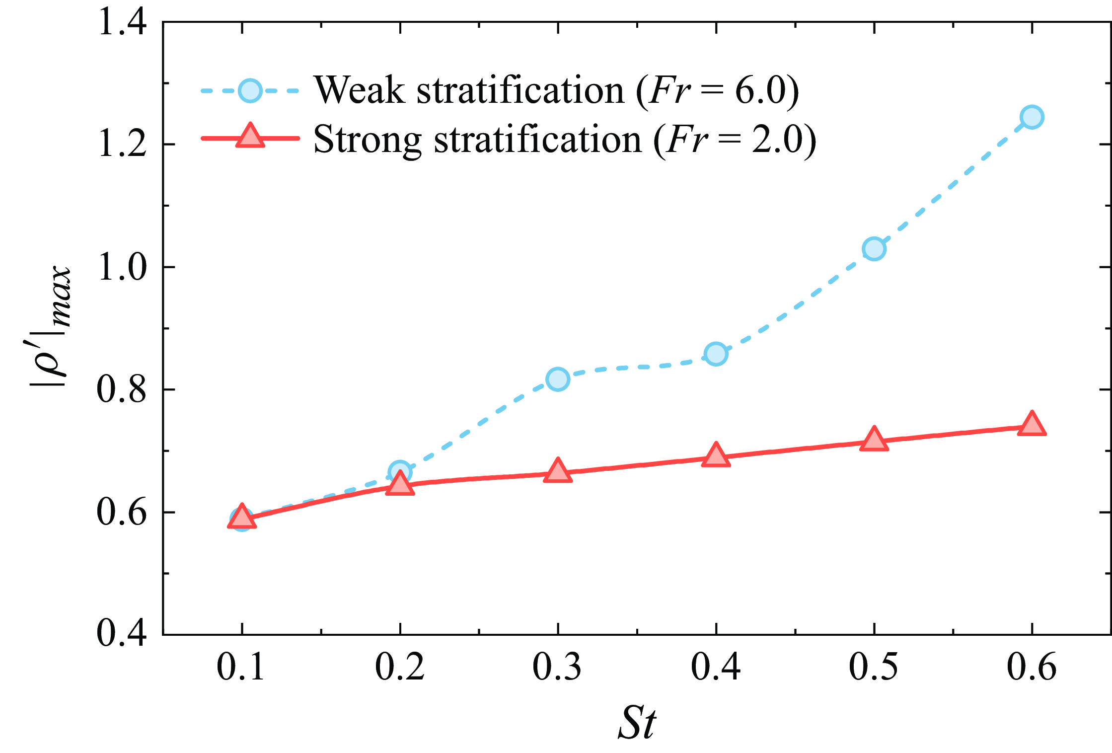
During the fluid entrainment, increasing Strouhal number amplifies density transport. Figure 17 shows the maximum density perturbation magnitude at
 $t = T$
for different Strouhal numbers. The results indicate that, in weakly stratified fluids, the intensity of density motion increases nonlinearly with
 $St$
, owing to the combined effects of flow inertia and buoyancy forces on density spreading. In strongly stratified fluids, however, a nearly linear increase in maximum density disturbance is observed as
 $St$
becomes higher, with buoyancy effects exclusively governing density perturbation. The magnitude of density transport at
 $Fr = 6.0$
is notably higher than that at
 $Fr = 2.0$
, especially for high Strouhal numbers. This behaviour is expected, as stronger stratifications provide greater resistance to vertical motions (Magnaudet & Mercier Reference Magnaudet and Mercier2020; More & Ardekani Reference More and Ardekani2023).
Variation of maximum density perturbation magnitude as a function of Strouhal number for different stratification strengths.

Influence of Strouhal number on instantaneous density field
 $\rho '$
for (
 $a$
–
 $c$
)
 $Fr = 6.0$
and (
 $d$
–
 $f$
)
 $Fr = 2.0$
. The spreading tendency and magnitude of density perturbation are illustrated by the direction and thickness of arrows.

Figure 18 depicts the effect of the Strouhal number on the instantaneous density field at
 $t = T$
. The direction and thickness of arrows illustrate the orientation and intensity of density spreading, respectively. We can see that stronger foil oscillations result in a wider scope of density transport. For
 $Fr = 6.0$
, inertial effects convey the enhanced density perturbation towards regions far from the body as
 $St$
increases, as shown by blue arrows in figures 18(
 $a$
)–18(
 $c$
). By comparison, the significant buoyancy effects at
 $Fr = 2.0$
, which promote the entrained fluids returning to their neutrally buoyant position, confine the amplifying density disturbance to the vicinity of the oscillating foil as
 $St$
increases, as shown by red arrows in figures 18(
 $d$
)–18(
 $f$
). The amplification of density disturbance near the foil is beneficial to thrust production at this stage, as discussed in figures 11 and 14. However, when the foil approaches the drag-produced phase (
 ${t_1} \lt t \lt {t_2}$
), this
 $St$
-induced amplification, sufficiently inhibited by pronounced buoyancy effects in strongly stratified fluids, becomes detrimental to thrust performance, as indicated in figures 12, 13 and 14. In summary, the strong stratifications can effectively capitalise on the amplification of density motion during the asymmetric fluid entrainment, which is a leading mechanism responsible for the notably high optimal
 $St$
observed in strongly stratified fluids.
5. Stratification-induced wake dynamics
In addition to hydrodynamic performance, another aspect in which the Strouhal number plays an important role is the wake dynamics. It has been well documented that an oscillating foil with different Strouhal numbers can generate a wide variety of wake patterns in homogeneous fluids (Schnipper et al. Reference Schnipper, Andersen and Bohr2009; Andersen et al. Reference Andersen, Bohr, Schnipper and Walther2017; Verma & Hemmati Reference Verma and Hemmati2022). In a stratified fluid, the baroclinic torque arising from isopycnal deflection can alter vorticity evolution, yielding flow patterns that differ from those in homogeneous fluids. Specifically, the wake structures under the stratification influence are governed by buoyancy effects, which inhibit the vertical motion while promoting the horizontal motion (Riley & Lelong Reference Riley and Lelong2000), and by induced internal waves that significantly impact the transport of energy and momentum (Staquet & Sommeria Reference Staquet and Sommeria2002). Given that the wake dynamics of oscillating foils in stratified regimes is largely unexplored, we provide an analysis regarding the role of Strouhal number in the stratified wake behaviours in this section.
It should also be noted that, despite extensive efforts in correlating propulsive performance with flow features, the intrinsic relationship between them remains complex and often inconsistent. Godoy-Diana et al. (Reference Godoy-Diana, Aider and Wesfreid2008) observed that the wake transition from a typical von Kármán street, associated with drag generation, to a reverse von Kármán street, indicative of thrust production, precedes the drag–thrust transition. Smits (Reference Smits2019) further indicated that wake dynamics and propulsive performance should be treated as two distinct yet interrelated topics, because efficient swimming may correspond to multiple different wake patterns. Such perspective is echoed by Eloy (Reference Eloy2012), Zhang (Reference Zhang2017) and Taylor (Reference Taylor2018), who suggested that efficient flow patterns are more likely to be a consequence of efficient propulsion, and caution should be exercised when employing wake development to explain propulsive performance. Therefore, rather than seeking to build a one-to-one connection between propulsive performance and wake structure, we mainly aim to map out the wake types across the (
 $St$
,
 $Fr$
) plane and offer novel insights into flow patterns in stratified environments.
5.1. Vortex structures
As a basis for comparison, figure 19 shows the wake evolution of a harmonically heaving and pitching foil across different Strouhal numbers in a homogeneous fluid. From figure 19(
 $a$
), we observe a 2P wake at
 $St = 0.10$
, which transitions into a 2S reverse von Kármán wake as the Strouhal number increases to
 $St = 0.20$
(see figure 19
 $b$
). According to the terminology by Williamson & Roshko (Reference Williamson and Roshko1988), 2P and 2S respectively denote two vortex pairs and two single vortices shed per oscillation cycle. As the Strouhal number further increases, the reverse von Kármán wake becomes more coherent in its spatial arrangement, as depicted in figure 19(
 $c$
–
 $f$
). These typical wake patterns are commonly observed in both experimental measurements and numerical simulations of homogeneous fluids (Schnipper et al. Reference Schnipper, Andersen and Bohr2009; Andersen et al. Reference Andersen, Bohr, Schnipper and Walther2017).
Instantaneous vorticity contours, normalised by
 ${U_\infty }/c$
, at (
 $a$
)
 $St = 0.10$
, (
 $b$
)
 $St = 0.20$
, (
 $c$
)
 $St = 0.30$
, (
 $d$
)
 $St = 0.40$
, (
 $e$
)
 $St = 0.50$
and (
 $f$
)
 $St = 0.60$
for a homogeneous fluid (
 $Fr = \infty$
). The flow pattern in a homogeneous fluid experiences a typical transition from 2P wake to 2S wake with the Strouhal number.

Figure 20 presents the evolution of wake configuration with
 $St$
in a weakly stratified fluid (
 $Fr = 6.0$
). Due to the generation of internal waves, the consecutive wave beams are evident in the flow pattern around the oscillating foil. When foil motion is weak, the wake pattern is characterised by a dispersed configuration, as shown in figure 20(
 $a$
). As the Strouhal number increases, the flow pattern evolves into a structure consisting of a central wake moving along the centreline and two symmetric oblique wakes deflecting outward (see figure 20
 $b$
,
 $c$
). Further increase in the Strouhal number leads to the merging of the central and oblique wakes, resulting in a chaotic flow pattern behind the oscillating foil, as illustrated in figure 20(
 $d$
–
 $f$
). In addition, the wake configuration in weakly stratified fluids shows a downstream tendency due to the dominance of the free stream over the propagation of induced internal waves.
The variation of wake structures with
 $St$
in a strongly stratified fluid (
 $Fr = 2.0$
) is exhibited in figure 21. Notably, the flow pattern undergoes a transition from an asymmetric arrangement at low Strouhal numbers to a symmetric configuration at high Strouhal numbers. The prominence of internal waves also increases with the strength of stratification. The growing influence of internal waves prompts vortex disturbances to spread towards the upstream region, giving rise to a radial flow pattern in strongly stratified conditions. The formation of wake patterns in a stratified regime depends on several factors, including the foil–vortex interplay, the vortex–vortex intertwining, and the interaction between internal waves and background mean flow. Especially, the wave–mean flow interaction, which irreversibly transfers energy to smaller scales, plays a critical role in the wake dynamics of stratified fluids (Staquet & Sommeria Reference Staquet and Sommeria2002; Howland et al. Reference Howland, Taylor and Caulfield2021). Both stronger foil motion and increasing stratification strength facilitate this process. Consequently, at high Strouhal numbers and low Froude numbers, the near wake becomes considerably disordered, as seen in figure 21(
 $f$
). Our previous study (Wang et al. Reference Wang, Kandel and Deng2024), which focused on
 $St = 0.30$
, provided a detailed illustration on the formation process of wake patterns in a stratified fluid medium.
Instantaneous vorticity contours at (
 $a$
)
 $St = 0.10$
, (
 $b$
)
 $St = 0.20$
, (
 $c$
)
 $St = 0.30$
, (
 $d$
)
 $St = 0.40$
, (
 $e$
)
 $St = 0.50$
and (
 $f$
)
 $St = 0.60$
for a weakly stratified fluid (
 $Fr = 6.0$
). Contour colours are the same as in figure 19. The flow pattern in a weakly stratified fluid exhibits a downstream tendency.

Instantaneous vorticity contours at (
 $a$
)
 $St = 0.10$
, (
 $b$
)
 $St = 0.20$
, (
 $c$
)
 $St = 0.30$
, (
 $d$
)
 $St = 0.40$
, (
 $e$
)
 $St = 0.50$
and (
 $f$
)
 $St = 0.60$
for a strongly stratified fluid (
 $Fr = 2.0$
). Contour colours are the same as in figure 19. The flow pattern in a strongly stratified fluid exhibits a radial tendency.

It can also be seen from figures 20 and 21 that the inhomogeneous background density distribution does not change the general wake symmetry about the centreline. For a linearly stratified fluid governed by Boussinesq equations, the density perturbation only depends on the background density gradient
 $\gamma$
, as illustrated by (2.10). Because
 $\gamma$
is constant throughout the whole domain, there is no dynamical distinction between upward and downward density perturbations (Sutherland Reference Sutherland2010). Consequently, the flow patterns retain an overall symmetry about the centreline. Such symmetric wakes about the horizontal axis in a linearly stratified fluid have been widely observed by both numerical simulations and experimental measurements (Chongsiripinyo et al. Reference Chongsiripinyo, Pal and Sarkar2017; Madison et al. Reference Madison, Xiang and Spedding2022; Ortiz-Tarin et al. Reference Ortiz-Tarin, Nidhan and Sarkar2023). However, due to the distortion of vortex structures by stratification effects, conventional wake classification symbols introduced by Williamson & Roshko (Reference Williamson and Roshko1988) are inadequate for describing wake types in stratified fluids. In this study, we classify wake types based on the spatial extent and concentration regions of vortex disturbances. As shown in figure 22, five representative flow patterns are identified within the parameter space defined by
 $St$
and
 $Fr$
.
(
 $a$
–
 $e$
) Instantaneous vorticity contours showing typical flow patterns generated by an oscillating foil in stratified fluids. (
 $f$
) Comparison between asymmetric (
 $St = 0.15$
,
 $Fr = 2.0$
) and symmetric (
 $St = 0.60$
,
 $Fr = 3.0$
) wakes behind an oscillating foil in stratified fluids. Contour colours are the same as in figure 19.

Flow pattern I is characterised by a radial configuration centred on the oscillating foil, with primary vortex disturbance concentrated around the body (figure 22
 $a$
). Flow pattern II presents the vorticity concentration only appearing in the downstream region behind the foil’s leading edge (figure 22
 $b$
). Flow pattern III exhibits a shuttle shape in which vorticity concentrates along the centreline both upstream and downstream (figure 22
 $c$
). Pattern IV is similar to pattern III but features a bifurcated downstream vortex concentration, leading to a larger vertical scale (figure 22
 $d$
). Flow pattern V displays a triangular configuration, with vortex disturbance aggregating downstream (figure 22
 $e$
). In addition, stratification effects induce a symmetry breaking in the wake as
 $St$
and
 $Fr$
vary. Figure 22(
 $f$
) contrasts asymmetric and symmetric wakes under these conditions.
Figure 23 provides a map of flow patterns in the (
 $St$
,
 $Fr$
) plane. The regime with low
 $Fr$
is dominated by flow pattern I, due to the significant influence of induced internal waves. As stratification weakens, the Strouhal number starts to play a comparable role in wake evolution. As a result, the regime with
 $St \leqslant 0.20$
is represented by flow pattern II, while pattern III occupies the regime with
 $St \gt 0.20$
. The combination of intense foil motion (high
 $St$
) and strong stratification (low
 $Fr$
) leads to an isolated regime in the lower-right corner of the wake map, characterised by flow pattern IV. Another distinct regime, defined by high
 $Fr$
and moderate
 $St$
, corresponds to flow pattern V, resulting from the dominant influence of background mean flow under extremely weak stratifications.
Flow pattern map for an oscillating foil in stratified fluids. The pattern types correspond to the vorticity contours in figure 22. The blue dashed line indicates the wake transition from asymmetry (lower-left regime) to symmetry (upper-right regime). The black solid line corresponds to the optimal Strouhal numbers at different levels of stratification.

The blue dashed line in figure 23 separates the flow pattern map into a lower-left regime, where asymmetric wakes dominate, and an upper-right regime, where symmetric wakes prevail. Generally, weak foil motion coupled with strong stratification tends to break wake symmetry, while higher
 $Fr$
and
 $St$
values favour the formation of symmetric wakes. These results are expected to offer a phase diagram of wake characteristics in stratified environments, enabling a comparison with homogeneous observations (Godoy-Diana et al. Reference Godoy-Diana, Aider and Wesfreid2008; Schnipper et al. Reference Schnipper, Andersen and Bohr2009; Andersen et al. Reference Andersen, Bohr, Schnipper and Walther2017).
Figure 23 also illustrates the variation of optimal Strouhal numbers in the (
 $St$
,
 $Fr$
) plane, as indicated by the black solid line. For weak stratifications, the optimum efficiency is observed at a higher
 $St$
than the value of wake transition. This observation is consistent with the previous study on an oscillating foil in homogeneous fluids (Deng et al. Reference Deng, Sun, Teng, Pan and Shao2016). However, in strongly stratified fluids, we find that the optimal condition of efficiency performance aligns with the wake transition point, indicating a synchronisation between the foil’s kinematics and flow disturbances. This behaviour presumably echoes earlier discussion regarding the inherent coupling between oscillatory frequency of the foil and Brunt–Väisälä frequency of stratified fluids.
One of the most striking features of flow patterns produced by a moving body in a stably stratified fluid is the presence of internal waves, as shown in figures 20–22. Lighthill (Reference Lighthill1967) developed a general theory that describes the generation of anisotropic dispersive waves by travelling disturbances. Stevenson & Thomas (Reference Stevenson and Thomas1969) performed a series of experiments on internal wave patterns induced by a horizontally moving cylinder with forced oscillation and found that their results are in good agreement with Lighthill’s theory. Subsequent studies by Rehm & Radt (Reference Rehm and Radt1975) and Voisin (Reference Voisin1994) further confirmed the validity of Lighthill’s theory in predicting internal wave patterns generated by translating and oscillating sources.
Comparison of internal wave patterns between numerical simulations and theoretical predictions at
 $Fr = 8.0$
: (
 $a$
) and (
 $b$
)
 $\Omega = 0.402$
, and (
 $c$
) and (
 $d$
)
 $\Omega = 1.608$
. The simulations in panels (
 $a$
) and (
 $c$
) show the vorticity field, normalised by
 ${U_\infty }/c$
with the range from -0.2 to 0.2. The predictions by Lighthill’s theory (Lighthill Reference Lighthill1967) presented in panels (
 $b$
) and (
 $d$
) show the curves of constant phase for internal waves (such as wave crests), in which the dashed lines represent the wave system from steady motion (
 $\Omega = 0$
) and the solid lines depict waves induced by oscillation.

Here, we compare the internal wave patterns obtained from our numerical simulations with the predictions of Lighthill’s theory, as shown in figure 24. Specifically, we examine the case of
 $Fr = 8.0$
with a constant Brunt–Väisälä frequency and body velocity. By varying the oscillatory frequency of the foil, we analyse two distinct scenarios:
 $\Omega \lt 1$
(
 $\Omega = 0.402$
) and
 $\Omega \gt 1$
(
 $\Omega = 1.608$
). For a translating body with forced oscillation, the wave system induced by the oscillation is superimposed on the steady wave system, which remains stationary relative to the oscillatory source (Stevenson & Thomas Reference Stevenson and Thomas1969). According to Lighthill’s theory, the wave system generated by steady motion consists of a series of semicircles centred on the body, whereas the oscillatory wave system exhibits different patterns depending on
 $\Omega$
. When
 $\Omega \lt 1$
, the oscillatory wave system displays a radial pattern propagating both upstream and downstream. In contrast, when
 $\Omega \gt 1$
, this system transitions into a wedge-shaped pattern trailing behind the oscillating body. Both the radial wave pattern (figure 24
 $b$
) and the wedge-shaped wave pattern (figure 24
 $d$
) are accurately captured in the simulations (figure 24
 $a$
,
 $c$
). Notably, the wave spacing observed in our numerical simulations aligns closely with theoretical predictions.
Despite this agreement, certain discrepancies are evident between the two results. The vortex shedding from the trailing edge of the foil in the simulations induces chaotic wave patterns in the downstream region near the body, which are absent in the theoretical predictions. Additionally, the numerical wave patterns along the centreline exhibit significant distortion, which notably deviates from theoretical expectations. This discrepancy arises because nonlinear effects, such as wave interactions and wave breaking, are not fully captured by Lighthill’s theory, which is based on linear assumptions. In contrast, our numerical simulations inherently account for these nonlinear phenomena.
5.2. Velocity profiles
Contours of time-averaged streamwise velocity, normalised by the free stream velocity
 $U_\infty$
, at varying Strouhal numbers for (a)
 $Fr = \infty$
(homogeneous case), (b)
 $Fr = 6.0$
and (c)
 $Fr = 2.0$
. The initial position of the foil’s trailing edge is located at the left boundary of each plot.

We further investigate the velocity distribution in stratified fluids. Figure 25 compares the contours of time-averaged streamwise velocity between homogeneous and stratified cases. In the homogeneous case (figure 25
a), the mean velocity field displays an energetic momentum jet behind the oscillating foil, generated by the reverse von Kármán vortex street (figure 19). As
 $St$
increases, a noticeable intensification in both magnitude and scope is observed in the near-wake jet. At the highest Strouhal number studied (
 $St = 0.60$
), the momentum jet exhibits a tendency of bifurcation in the vicinity of the foil. Note that the velocity jet is typically considered as a key indicator of thrust production in homogeneous studies (Dewey et al. Reference Dewey, Carriou and Smits2012; Quinn et al. Reference Quinn, Moored, Dewey and Smits2014; Verma & Hemmati Reference Verma and Hemmati2022).
Figures 25(b) and 25(c) show the time-averaged velocity contours in weakly and strongly stratified fluids, respectively. In these stratified conditions, the velocity distribution is characterised by a central momentum excess region flanked by diverging velocity streams. These streams are noted to follow the pattern of internal waves, manifesting as alternating velocity excess and deficit streaks. Similar to the homogeneous case, stronger foil motion results in more energetic momentum jets in stratified fluids. Notably, the presence of internal waves induces a significant bifurcation in the central jet at
 $St = 0.60$
. For weak stratification, this bifurcated jet is interrupted by a velocity deficit region, as seen in figure 25(b). In contrast, under strong stratification, the velocity deficit region splits the jet along the centreline into two streams near the foil, which eventually merge into a single jet further downstream (figure 25
c). This difference is attributed to varying wave frequencies in weakly and strongly stratified fluids. The central momentum jet under weak stratification is comparable to that in the homogeneous case, but only near the foil’s trailing edge. Given the similar level of thrust production between weakly stratified and homogeneous cases (figure 5
a), it suggests that the near-wake velocity jet is a more pivotal indicator of thrust performance, while far-wake velocity distribution is less significant. Interestingly, the central momentum jet in strongly stratified fluids is less energetic than that in homogeneous fluids, despite the higher thrust production at
 $Fr = 2.0$
compared with
 $Fr = \infty$
(figure 5
a). This implies that diverging velocity excess streams also contribute to thrust production, and these wave-induced velocity streaks must be fully considered when evaluating thrust through streamwise momentum flux.
We also quantitatively assess the mean velocity profiles in figures 26–28, focusing on the cross-stream line at five streamwise locations. The near-wake region is characterised by
 $x/c = 0.5$
,
 $x/c = 1.0$
,
 $x/c = 2.0$
and
 $x/c = 3.0$
, while
 $x/c = 10.0$
represents the far wake. In the homogeneous case (figure 26), the central jet with multiple velocity peaks dominates the wake, consistent with the observations in figure 25(a). Additionally, low Strouhal numbers cause wake bifurcation in the far wake (figure 26
e), whereas strong foil motion leads to bifurcation in the near wake (figure 26
a–d). In stratified regimes, the mean velocity distribution along the cross-stream line exhibits a wavy profile, with central primary peaks flanked by alternating minima and maxima (figures 27 and 28). These velocity minima and maxima, which decay downstream or away from the centreline, mirror the diverging velocity deficit and excess streams in figures 25(b) and 25(c). We see that the bifurcation of velocity distribution under stratification only occurs in the near wake. More specifically, the central velocity profile at weak stratification tends to bifurcate when
 $St$
exceeds a certain value, resembling the behaviour in homogeneous fluids (figure 27
a–d). In contrast, strong stratification consistently induces bifurcation along the centreline, independent of
 $St$
(figure 28
a–d).
Time-averaged streamwise velocity profiles with varying Strouhal numbers along the cross-stream line at streamwise locations of (
 $a$
)
 $x/c = 0.5$
, (
 $b$
)
 $x/c = 1.0$
, (
 $c$
)
 $x/c = 2.0$
, (
 $d$
)
 $x/c = 3.0$
and (e)
 $x/c = 10.0$
downstream of foil trailing edge for a homogeneous fluid (
 $Fr = \infty$
).

Time-averaged streamwise velocity profiles with varying Strouhal numbers along the cross-stream line at streamwise locations of (
 $a$
)
 $x/c = 0.5$
, (b)
 $x/c = 1.0$
, (
 $c$
)
 $x/c = 2.0$
, (
 $d$
)
 $x/c = 3.0$
and (
 $e$
)
 $x/c = 10.0$
downstream of foil trailing edge for a weakly stratified fluid (
 $Fr = 6.0$
).

Time-averaged streamwise velocity profiles with varying Strouhal numbers along the cross-stream line at streamwise locations of (
 $a$
)
 $x/c = 0.5$
, (
 $b$
)
 $x/c = 1.0$
, (
 $c$
)
 $x/c = 2.0$
, (
 $d$
)
 $x/c = 3.0$
and (
 $e$
)
 $x/c = 10.0$
downstream of foil trailing edge for a strongly stratified fluid (
 $Fr = 2.0$
).

As previously noted, increasing the Strouhal number significantly enhances the momentum jet behind the oscillating foil. However, this velocity enhancement manifests differently in homogeneous and stratified fluids. In the homogeneous case, the enhanced momentum flux is directed downstream, resulting in a uniform velocity distribution along the centreline (figure 25
 $a$
). Conversely, the stratification effects tend to concentrate the intensified momentum flux upstream, creating highly energetic velocity excess streams near the foil (see figures 25
 $b$
and 25
 $c$
). The quantitative results presented in figures 26–28 further confirm this behaviour. It is apparent from figure 26 that the peaks of velocity profiles in a homogeneous fluid consistently depend on the Strouhal number along the centreline. In stratified regimes, however, the variation of mean velocity profiles with the Strouhal number is evident only in the near wake, while the minima and maxima of velocity in the far wake are nearly independent of the Strouhal number (figures 27 and 28). More importantly, we observe a more energetic near wake at
 $Fr = 2.0$
compared with that of
 $Fr = 6.0$
, indicating an increased concentration of momentum flux with stronger stratification. This behaviour partly explains the significant thrust production and the notably high optimal Strouhal numbers in strongly stratified fluids.
6. Conclusions
This study numerically investigates the Strouhal number dependence of propulsive performance for a combined heaving and pitching foil in density stratified fluids. The results demonstrate that the optimal Strouhal number
 $S{t_m}$
is significantly influenced by stratification strength. For weak stratifications (
 $Fr \geqslant 5$
), the highest efficiency occurs at a Strouhal number similar to that observed in homogeneous fluids. However, as stratification strengthens (
 $Fr \lt 5$
), the optimal Strouhal number increases with decreasing
 $Fr$
, eventually exceeding the typical range of
 $0.20 \lt St \lt 0.40$
observed in homogeneous conditions. Notably, the strongest stratification in our parameter space yields an optimal Strouhal number of
 $S{t_m} = 0.59$
, significantly higher than those observed in homogeneous fluids. Our findings suggest an inherent coupling between oscillatory frequency of the foil and the Brunt–Väisälä frequency of the fluid. The highest efficiency in oscillatory propulsion occurs when resonance between the foil and fluid oscillations is triggered. A fitting formula based on this hypothesis accurately characterises the relationship between
 $S{t_m}$
and
 $Fr$
, indicating that resonance behaviour is a key factor driving the increase in
 $S{t_m}$
with stratification strength.
We further explore the hydrodynamic mechanisms underlying these observations. The results reveal that asymmetric fluid entrainment by foil oscillation plays a crucial role in achieving high optimal Strouhal numbers under strong stratifications. The oscillating foil drags a volume of fluid into regions with varying densities, inducing density perturbations governed by the relative magnitudes of inertial and buoyancy effects. In weakly stratified fluids, flow inertia tends to direct the density disturbances away from the foil, while in strongly stratified fluids, buoyancy forces restrict density transport to regions close to the foil. During fluid entrainment, increasing the Strouhal number facilitates density motion and amplifies density perturbations. We find that strong stratifications, associated with prominent buoyancy effects, can effectively exploit this
 $St$
-induced enhancement in density transport to create specific pressure distributions that benefit hydrodynamic performance. Consequently, in strongly stratified fluids, the streamwise component of instantaneous forces experiences a significant increase in peaks without a corresponding rise in drag generation as the Strouhal number increases. This behaviour contributes to a considerable improvement in cycle-averaged thrust production with increasing
 $St$
, leading to efficient propulsion at higher Strouhal numbers.
The wake dynamics of an oscillating foil in stratified regimes is another focus in this study. We first provide a map of flow patterns by identifying various wake types in the (
 $St$
,
 $Fr$
) plane. It is noted that in weakly stratified fluids, the optimal Strouhal numbers tend to precede the values of wake transition, consistent with previous observations in homogeneous cases. Interestingly, the optimal condition at strong stratifications agrees well with the wake transition, distinguishing it from the homogeneous observations. We then explore the streamwise velocity features under the effects of stratification. Unlike the uniform distribution of the velocity jet in homogeneous fluids, stratification effects concentrate the enhanced momentum flux to approach the oscillating foil at higher
 $St$
, resulting in highly energetic velocity excess streams in the near wake.
The findings of this study provide several new insights into oscillatory propulsion. First of all, some canonical optimisation procedures for homogeneous scenarios may not be applicable in stratified environments due to different optimal conditions. It is thus suggested that aquatic animals or artificial propulsors using oscillatory mechanisms should adopt different propulsion strategies to achieve efficient swimming in density stratified fluids. Additionally, an oscillating foil propulsor in strongly stratified fluids can attain optimum efficiency combined with considerable thrust production, avoiding the trade-off between thrust and efficiency commonly encountered in homogeneous cases. Moreover, the influence of stratification should be fully taken into consideration when using simple rules of thumb based on optimal Strouhal numbers to predict the cruising speed of aquatic animals. In this context, we retain the possibility that the presence of density stratification contributes to the surprisingly large Strouhal numbers observed in several natural swimmers, as oceans are inherently stratified.
Funding.
This research has been supported by the Zhejiang Provincial Natural Science Foundation of China under Grant No. LZ25A020003 and the National Natural Science Foundation of China (Grants No. 92252102 and No. 92152109).
Declaration of interests.
The authors report no conflict of interest.
Appendix. Verification of temporal and spatial independence
A sensitivity study is conducted to demonstrate the time, grid and domain independence of the computational code used in this study. Here, we consider the most extreme case with the strongest foil motion (
 $St = 0.6$
) and highest stratification strength (
 $Fr = 1.0$
) in the current parameter space.
Time series of the instantaneous (a) thrust coefficient and (b) lift coefficient at
 $St = 0.6$
for
 $Fr = 1.0$
showing temporal independence by different time step resolutions.

Time series of the instantaneous (a) thrust coefficient and (b) lift coefficient at
 $St = 0.6$
for
 $Fr = 1.0$
showing spatial independence by different grid resolutions.

Time sensitivity is first assessed by testing four different time steps:
 $\Delta {t_1} = T/1000$
,
 $\Delta {t_2} = T/2000$
,
 $\Delta {t_3} = T/4000$
and
 $\Delta {t_4} = T/8000$
. Figure 29 shows the time histories of the instantaneous thrust and lift coefficients at different temporal resolutions. The results are found to be insensitive to temporal resolution when the number of time steps per oscillation cycle exceeds 4000. The temporal resolution of
 $\Delta {t_3} = T/4000$
is therefore used to run all the simulations in the present study. We then assess the grid sensitivity. By varying the number of grid points on the foil surface and modifying the normal grid spacing, we examine four spatial resolutions: Grid 1 with 122 074 elements, Grid 2 with 203 481 elements, Grid 3 with 343 105 elements and Grid 4 with 574 553 elements. The time series of force coefficients, as shown in figure 30, indicate excellent agreement between Grid 3 and Grid 4 with the largest deviation being less than 0.5 %. Therefore, we use spatial resolution Grid 3 to perform all the computations due to its satisfactory accuracy in space.
Time series of the instantaneous (a) thrust coefficient and (b) lift coefficient at
 $St = 0.6$
for
 $Fr = 1.0$
showing domain independence by different domain sizes.

For numerical simulations of stratified fluids, the computational domain needs to be large enough to avoid the interactions between body and waves reflected from the boundaries. Here, we test four domain sizes to verify the independence of the computational domain. Figure 31 shows the force variations using the domain sizes
 $50c \times 50c$
,
 $100c \times 100c$
,
 $150c \times 150c$
and
 $200c \times 200c$
, respectively. The maximum difference between the domain sizes
 $100c \times 100c$
and
 $150c \times 150c$
is 1.72 % in the instantaneous thrust coefficient
 $C_t$
and 0.85 % in the instantaneous lift coefficient
 $C_l$
. The deviation in the cycle-averaged thrust coefficient
 $C_T$
between the domain sizes
 $50c \times 50c$
and
 $100c \times 100c$
is 5.22 %, which decreases to 1.79 % when comparing the domain sizes
 $100c \times 100c$
and
 $150c \times 150c$
. Considering the trade-off between accuracy and computational cost, we select the domain size
 $100c \times 100c$
for all cases in this study.