



1. Introduction
Schooling behaviour, or collective motion, is commonly observed in biological systems in nature (e.g. fish schooling and birds flocking) (Weihs Reference Weihs1973; Portugal et al. Reference Portugal, Hubel, Fritz, Heese, Trobe, Voelkl, Hailes, Wilson and Usherwood2014). When groups of active animals move in a fluid, the locomotion of each is influenced by those of the others through the flow-mediated interactions among them, and individuals in a schooling formation gain an energetic advantage in light of their hydrodynamics (Weihs Reference Weihs1973; Hemelrijk et al. Reference Hemelrijk, Reid, Hildenbrandt and Paddling2015; Weihs & Farhi Reference Weihs and Farhi2017). Furthermore, flying/swimming organisms can take advantage of hydrodynamic benefits when they move near a wall (a phenomenon commonly called the ‘wall effect’). Examples include buoyant mandarin fish and brown pelicans (Blake Reference Blake1979; Hainsworth Reference Hainsworth1988). Because the flow decelerates beneath a rigid or flexible body near a wall, greater pressures on the underside can generate more lift force via the wall effect. Despite individual studies of self-propelled propulsors in a school (Zhu, He & Zhang Reference Zhu, He and Zhang2014a; Park & Sung Reference Park and Sung2018; Peng, Huang & Lu Reference Peng, Huang and Lu2018a,Reference Peng, Huang and Lub,Reference Peng, Huang and Luc) and a single self-propelled propulsor with regard to wall effects (Dai, He & Zhang Reference Dai, He and Zhang2016; Park, Kim & Sung Reference Park, Kim and Sung2017; Zhang, Huang & Lu Reference Zhang, Huang and Lu2017), a hydrodynamic approach to schooling behaviours as influenced by walls has yet to be conducted.
As a typical schooling formation, passive and active responses of two tandem flapping bodies in a uniform flow were initially studied in tethered systems (Ristroph & Zhang Reference Ristroph and Zhang2008; Zhu Reference Zhu2009; Kim, Huang & Sung Reference Kim, Huang and Sung2010; Boschitsch, Dewey & Smits Reference Boschitsch, Dewey and Smits2014; Uddin, Huang & Sung Reference Uddin, Huang and Sung2015). Here, the tandem arrangement indicates that two or more objects are located in line with the flow or moving direction. However, because individuals in groups do not change their positions by instantaneously reacting to the surrounding flow in the system, self-propelled tandem models with heaving motions have been developed to reflect reality (Zhu et al. Reference Zhu, He and Zhang2014a; Becker et al. Reference Becker, Masoud, Newbolt, Shelley and Ristroph2015; Ramananarivo et al. Reference Ramananarivo, Fang, Oza, Zhang and Ristroph2016). When two self-propelled tandem rigid foils move along the horizontal direction with a prescribed (fixed) horizontal gap distance between them, Becker et al. (Reference Becker, Masoud, Newbolt, Shelley and Ristroph2015) found that such foils in a quiescent flow select slow and fast modes, corresponding to constructive and destructive vortex–body interactions, respectively. Furthermore, when the speed and horizontal gap spacing of two self-propelled flexible fins in a tandem arrangement can be freely selected, Zhu et al. (Reference Zhu, He and Zhang2014a) showed that two stable configurations (i.e. compact and sparse) are formed spontaneously from the help of a leader through a shared fluid environment. In the compact configuration, the two fins behaved as one long fin while maintaining a narrow gap distance between them; they swam faster than an isolated fin, although they consumed more power. In the sparse configuration, where a follower swims in a reverse von Kármán vortex street generated by a leader while maintaining a sufficiently long distance, the trajectory of the follower was locked onto vortex cores generated by the leader, which is referred to as the vortex interception mode (or vortex locking phenomenon). For two self-propelled tandem rigid foils, Ramananarivo et al. (Reference Ramananarivo, Fang, Oza, Zhang and Ristroph2016) also found the vortex interception mode experimentally, and they reported that the sparse configuration which emerges passively from hydrodynamic interactions without the need for collective decision making or active control mechanisms supports the Lighthill conjecture (Lighthill Reference Lighthill1975). However, in a von Kármán vortex street shed from an upstream object (e.g. stationary solid body and passively flapping fin), a flexible fin downstream is known to pass between vortex cores, i.e. the slalom mode (Liao et al. Reference Liao, Beal, Lauder and Triantafyllou2003; Jia & Yin Reference Jia and Yin2008; Uddin et al. Reference Uddin, Huang and Sung2015). Very recently, Newbolt, Zhang & Ristroph (Reference Newbolt, Zhang and Ristroph2019) examined the collective locomotion of two tandem rigid foils with different flapping kinematics (i.e. the heaving amplitude or flapping frequency), showing that a weakly flapping follower keeps pace with a more rapidly flapping leader by surfing on the oncoming wake.
Aside from the simple two tandem foil/fin systems, complex multiple (more than two) fin systems with different fin properties and configurations have been studied to investigate the general schooling principle. When two self-propelled fins are arranged with a close lateral distance between them in a compact configuration, Peng et al. (Reference Peng, Huang and Lu2018a) found that the two fins achieve high propulsive efficiency compared to an isolated fin at a moderate bending rigidity. Because the flexible deformation redistributed the total normal force into the moving direction (i.e. enhancement of the horizontal component of a normal force), a thrust force acting on the flexible fins was enhanced by a proper flexibility of the fins, compared to that acting on rigid fins. However, when the fins were highly flexible, a weak structural restoring force led to a low total force due to compliance of the fins with the fluid force, thereby reducing the thrust force. To examine the inherent hydrodynamic drafting mechanism of self-propelled fins with different fin properties, e.g. a mother–calf pair of dolphins, Peng et al. (Reference Peng, Huang and Lu2018c) investigated the schooling behaviours of two self-propelled fins with different fin lengths and bending rigidities. The propulsive performance of a fin with a weak propulsive capacity (i.e. a short fin) was improved when it followed a fin with a strong propulsive capacity (i.e. a long fin) in a school. Motivated by an earlier study by Weihs (Reference Weihs1973), Park & Sung (Reference Park and Sung2018) explored the collective dynamics of four self-propelled flexible fins in a diamond configuration. They found that the propulsive efficiency of the following fin increases because the increased circulation of vortices shed from three leading fins induces a strong lateral flow, and the follower can keep pace with the leaders even when using reduced heaving amplitudes with the assistance of the vortex street behind the leaders. Finally, Peng et al. (Reference Peng, Huang and Lu2018b) studied the collective behaviour of multiple self-propelled fins, up to eight fins in their study, in a tandem configuration. They showed that the entire group of multiple fins can consist of subgroups and/or individuals depending on the initial gap distance, and also that compact and sparse configurations are determined by the formation of subgroup(s) by the leading fins.
It is known that the swimming/flying of fish and birds (e.g. dark-edged-wing flying fish, brown pelicans and black skimmers) near a wall can have hydrodynamic benefits (Baudinette & Schmidt-Nielsen Reference Baudinette and Schmidt-Nielsen1974; Withers & Timko Reference Withers and Timko1977; Hainsworth Reference Hainsworth1988; Park & Choi Reference Park and Choi2010). The existence of the wall influences both the locomotion of the fin and the wake structures, with complex fluid–structure interactions. Significant efforts using experiments and numerical simulations have been devoted to the study of the passive or active locomotion of a tethered single rigid foil or a flexible fin near a wall (Blevins & Lauder Reference Blevins and Lauder2013; Quinn, Lauder & Smits Reference Quinn, Lauder and Smits2014a; Quinn et al. Reference Quinn, Moored, Dewey and Smits2014b). However, only a few numerical studies have been conducted to investigate the self-propulsion mechanisms of a freely movable isolated flexible fin with a constrained lateral heaving motion near a wall (Dai et al. Reference Dai, He and Zhang2016; Park et al. Reference Park, Kim and Sung2017; Zhang et al. Reference Zhang, Huang and Lu2017). When the fin is free to move in the horizontal direction, Dai et al. (Reference Dai, He and Zhang2016), Park et al. (Reference Park, Kim and Sung2017) and Zhang et al. (Reference Zhang, Huang and Lu2017) found that the cruising speed and propulsive efficiency of the fin are enhanced near the wall, although the input power increases or decreases according to the heaving amplitude and bending rigidity. Furthermore, they showed that a moderate bending rigidity and mass ratio can improve the cruising speed and propulsive efficiency in the wall effect. Using a numerical and experimental set-up for a freely movable isolated rigid pitching foil in the lateral direction, Kurt et al. (Reference Kurt, Cochran-Carney, Zhong, Mivehchi, Quinn and Moored2019) found that the foil near a wall spontaneously settles on a stable equilibrium altitude, where the time-averaged lateral force is zero, and the thrust force is enhanced with high efficiency at the equilibrium position compared to that far from the wall. In addition to a pitching rigid foil, the existence of a stable equilibrium altitude has been identified for a passively flapping fin, which is free to move in the lateral direction (Jeong & Lee Reference Jeong and Lee2018).
The objective of the present study is to examine the schooling behaviour of two self-propelled tandem flexible fins influenced by walls. The introduction of wall effects when used in conjunction with dynamically moving fins in a school results in more complicated flow-mediated interactions between them compared to the interactions without wall effects (Zhu et al. Reference Zhu, He and Zhang2014a). In order to examine the collective dynamics created by a long-range flow interaction in which the propulsive properties of the leader are scarcely affected by the follower, we consider a sparse configuration for the two tandem fins (Zhu et al. Reference Zhu, He and Zhang2014a; Becker et al. Reference Becker, Masoud, Newbolt, Shelley and Ristroph2015; Ramananarivo et al. Reference Ramananarivo, Fang, Oza, Zhang and Ristroph2016). Furthermore, the wall effects on the flow-mediated interaction are investigated using both a single wall and two parallel walls on the bottom and top. Although a single wall is typically employed to examine the wall effects on the hydrodynamics, the configuration of the two parallel walls has also been observed not only in the natural habitat of stream fish (e.g. rainbow trout, brown trout and coho salmon) but also during the long-distance migration of salmonid fish (e.g. Atlantic salmon) when they swim near vertical structures such as stream margins, rock faces and large woody debris (Menzies & Shearer Reference Menzies and Shearer1957; Feldmeth & Jenkins Reference Feldmeth and Jenkins1973; Fausch Reference Fausch1984; Webb Reference Webb1993).
Below, we analyse the vortex structures generated by a single isolated fin with and without wall effects to highlight the propulsive characteristics of the fin (§ 3.1), after which the propulsive mechanism of the schooling fins with wall effects is investigated to address the following two main questions: (i) How does the follower interact with the vortex structures generated by the leader under the influence of walls, and (ii) how do flow-mediated interactions improve the propulsive efficiency of schooling fins near walls? Based on the time histories of the average lateral velocity of the fin, the temporal input power and the average lateral flow acting on the fin in § 3.2, we show that the time-averaged input power of the follower with wall effects is significantly reduced by strong synchronized lateral flow compared to that without the wall. Although the time-averaged input power of the follower with and without wall effects is smaller than that of the leader, the enhanced flapping amplitude of the follower and anti-synchronization between the lateral flow generated by the leader and the lateral motion of the follower lead to an increase of temporal input power as a penalty. Furthermore, we show that the horizontal component of the normal force (i.e. thrust force) acting on the follower under wall effects reduces due to the help of a negative horizontal flow generated by the interaction between the main vortex and induced vortex near the wall, although the presence of a strong jet-like flow (i.e. positive horizontal flow) without wall effects requires a large amount of a thrust force on the follower. After analysing the underlying characteristics of the fluid-mediated interactions, we show that change of the flapping mode in wall effects is a necessary step to adapt to different vortical environments for the efficient propulsion of the follower (i.e. vortex interception mode with no wall to mixed and slalom modes near a single wall and between two parallel walls, respectively). Finally, we show in § 3.3 that the schooling efficiency is optimized with a small heaving amplitude of the follower and a critical value of the phase difference between the leader and follower when the values of the bending rigidity and wall proximity are moderate.
2. Numerical method
Figure 1 shows schematics of two self-propelled flexible fins in a tandem configuration with two coordinate systems for collective locomotion, when the fins propel near a single wall (figure 1a) and between two parallel walls (figure 1b). The upstream and downstream fins are denoted as the ‘leader’ and ‘follower’, respectively. Two flapping fins are driven by harmonic plunging motions at the leading edge with the heaving amplitude Ahead and flapping frequency f in the lateral direction, whereas the motion of the remaining parts is determined passively by the ambient fluid and nearby structures. In the horizontal direction, the fins are unconstrained and can thus move freely. The horizontal moving speed (i.e. cruising speed) and the horizontal relative positions between the leader and follower (Gx) are determined spontaneously as a result of the interaction between the flexible fin and the ambient fluid. The lateral distance between the fin and the wall (d), an important factor when determining the degree of the wall effect, is prescribed using the mean lateral position of the leading edge.
Schematic of two tandem flexible fins in a quiescent flow, when the fins propel (a) near a single wall and (b) between two parallel walls. The horizontal gap distance between two fins is denoted by Gx and the lateral distance between the equilibrium position of the heaving motion and the wall is denoted by d. The leading edges of the leader and follower are driven laterally by harmonic heaving motions, i.e. yl(t) and yf(t), and the fins can move freely in the horizontal direction.

To investigate the collective system of the self-propelled fins and the fluid flow, the viscous fluid flow is governed by the incompressible Navier–Stokes and continuity equations, i.e.
 \begin{gather}\frac{{\partial \boldsymbol{u}}}{{\partial t}} + \boldsymbol{u}\boldsymbol{\cdot} \boldsymbol{\nabla} \boldsymbol{u} ={-} {\bf \nabla }p + \frac{1}{{Re}}{\nabla ^2}\boldsymbol{u} + \boldsymbol{f},\end{gather}
 \begin{gather}\boldsymbol{\nabla} \boldsymbol{\cdot} \boldsymbol{u} = 0,\end{gather}
where the flapping Reynolds number Re is defined as  $Re = {U_{ref}}L/v$, with v representing the kinematic viscosity of the fluid. These governing equations are non-dimensionalized by the following characteristic scales: the fin length L for the length, the fluid density ρ 0 for the density, the maximum heaving velocity
 ${U_{ref}}( = 2{\rm \pi} f{A_{head,1}})$, where the subscript l indicates the leader (Zhu et al. Reference Zhu, He and Zhang2014a; Zhu, He & Zhang Reference Zhu, He and Zhang2014b; Dai et al. Reference Dai, He and Zhang2016; Peng et al. Reference Peng, Huang and Lu2018a,Reference Peng, Huang and Lub,Reference Peng, Huang and Luc), for the velocity u, L/Uref for the time t,
 ${\rho _0}U_{ref}^2$ for the pressure p and
 ${\rho _0}U_{ref}^2/L$ for the momentum forcing f. Using the fractional step method, (2.1) and (2.2) are solved in time in compliance with an implicit velocity-decoupling procedure (Kim, Baek & Sung Reference Kim, Baek and Sung2002). Both velocity–pressure decoupling and the decoupling of the intermediate-velocity components are achieved by block lower triangular-upper triangular (LU) decomposition with approximate factorization. Initially, the terms are discretized in time using the Crank–Nicolson method, after which the coupled velocity components are resolved without iterations. Using a second-order central difference scheme, all terms are solved in space with a staggered mesh.
The non-dimensional flexible fin motion under an inextensibility condition is described as follows (Huang, Shin & Sung Reference Huang, Shin and Sung2007):
 \begin{gather}\frac{{{\partial ^2}\boldsymbol{X}}}{{\partial {t^2}}} = \frac{\partial }{{\partial s}}\left( {\zeta \frac{{\partial \boldsymbol{X}}}{{\partial s}}} \right) - \frac{{{\partial ^2}}}{{\partial {s^2}}}\left( {\gamma \frac{{{\partial^2}\boldsymbol{X}}}{{\partial {s^2}}}} \right) - {\boldsymbol{F}_L},\end{gather}
 \begin{gather}\frac{{\partial \boldsymbol{X}}}{{\partial s}}\boldsymbol{\cdot }\frac{{\partial \boldsymbol{X}}}{{\partial s}} = 1,\end{gather}
where X = (X(s,t), Y(s,t)) represents the position vector of the fin and s is the Lagrangian variable defined along the fin (0 ≤ s ≤ 1). The motion equations of the inextensible flexible fin are non-dimensionalized by the following characteristic scales:  ${\rho _1}U_{ref}^2/L$ for the units of the Lagrangian momentum force FL,
 ${\rho _1}U_{ref}^2$ for the tension force ζ and
 ${\rho _1}U_{ref}^2/{L^2}$ for the bending rigidity γ, where ρ 1 denotes the density difference between the fin and the surrounding fluid. The tension force ζ is represented as a function of the Lagrangian variable s and time t and is determined from the inextensibility condition in (2.4). At the leading edge (s = 0) and trailing edge (s = 1), the following boundary conditions are applied:
 \begin{align} {y_l}(t) & = {A_{head,l}}\sin (2{\rm \pi} ft),\quad {y_f}(t) = {A_{head,f}}\sin (2{\rm \pi} ft + \phi ),\quad \dfrac{{\partial \boldsymbol{X}}}{{\partial s}} = (1,0),\nonumber\\ \dfrac{{{\partial ^3}X}}{{\partial {s^3}}} & = 0\,\textrm{at}\;s = 0, \end{align}
 \begin{align}\zeta &= 0,\quad \frac{{{\partial ^2}\boldsymbol{X}}}{{\partial {s^2}}} = (0,0),\quad \frac{{{\partial ^3}\boldsymbol{X}}}{{\partial {s^3}}} = (0,0) \,\textrm{at}\;s = 1,\end{align}
where the subscript f represents the follower and ϕ is the phase difference of the lateral position between the leader and follower. The boundary condition in (2.5) indicates the lateral harmonic heaving motion (2.5a,b), the clamped condition (2.5c) and the unconstrained condition in the horizontal direction (2.5d) (Hua, Zhu & Lu Reference Hua, Zhu and Lu2013; Zhu et al. Reference Zhu, He and Zhang2014a,Reference Zhu, He and Zhangb; Park & Sung Reference Park and Sung2018; Peng et al. Reference Peng, Huang and Lu2018a,Reference Peng, Huang and Lub,Reference Peng, Huang and Luc). The free-end condition in (2.6) is imposed at the trailing edge.
The Lagrangian momentum force between the flow and structure in (2.3) is obtained using the feedback force,
 \begin{equation}{\boldsymbol{F}_L}(s, t) ={-} \kappa [({\boldsymbol{X}_{ib}} - \boldsymbol{X}) + \varDelta t({\boldsymbol{U}_{ib}} - \boldsymbol{U})],\end{equation}
where κ is a large negative constant (κ = −2 × 10⁶), Δt denotes the computational time step (Δt = 0.00005) and the velocity of the fin U = (U(s,t), V(s,t)) is estimated by U = ∂X/∂t. In contrast, Xib and Uib are, respectively, the position and velocity obtained by interpolation at the immersed boundary. The following interpolation relationships between the Eulerian and Lagrangian variables are determined using the Dirac delta function,
 \begin{gather}{\boldsymbol{X}_{ib}} = \boldsymbol{X}_{ib}^0 + \int_0^t {{\boldsymbol{U}_{ib}}\,\textrm{d}t} ,\end{gather}
 \begin{gather}{\boldsymbol{U}_{ib}}(s,t) = \int_\varOmega {\boldsymbol{u}(\boldsymbol{x},t)\delta (\boldsymbol{X}(s,t) - \boldsymbol{x})\,\textrm{d}\boldsymbol{x}} ,\end{gather}
where Ω denotes the fluid region and δ( ) indicates a smoothed approximation of the Dirac delta function. The Eulerian momentum force f is calculated from the Lagrangian force FL using the smoothed delta function,
 \begin{equation}\boldsymbol{f}(\boldsymbol{x},t) = \mu \int_S {{\boldsymbol{F}_L}(s,t)\delta (\boldsymbol{x} - \boldsymbol{X}(s,t))\,\textrm{d}s} ,\end{equation}
where μ = ρ 1/ρ 0L represents the structure-to-fluid mass ratio and S is the structure region.
The computational domain normalized by the fin length L is 81.92 in the horizontal direction (−40.96 ≤ x ≤ 40.96). The domain size in the lateral direction is 8 for the no-wall and single-wall cases (−4 ≤ y ≤ 4 for the no-wall case and 0 ≤ y ≤ 8 for the single-wall case). For the case of the two parallel walls, the domain size is determined based on the lateral distance between the fin and the wall (d), with a constant grid spacing of 0.02, as shown in table 1. The Lagrangian grid size of the fin is 50. Tests of grid and domain sizes (that are performed independently) indicated that the influence of the sizes on our results is negligible (not shown). No-slip conditions are applied at the bottom wall for the single-wall case and both at the top and bottom walls for the case of the two parallel walls. Neumann boundary conditions are applied at the inlet and outlet (the front and rear sides of the fluid domain). In the entire computational domain, the fluid is quiescent with zero velocity at the initial time. The present numerical method was validated through a direct comparison with previous data for multiple fins (Park & Sung Reference Park and Sung2018), a single fin with wall effects (Park et al. Reference Park, Kim and Sung2017) and tethered fins (Huang et al. Reference Huang, Shin and Sung2007; Kim et al. Reference Kim, Huang and Sung2010; Uddin, Huang & Sung Reference Uddin, Huang and Sung2013; Uddin et al. Reference Uddin, Huang and Sung2015; Jeong & Lee Reference Jeong and Lee2017; Son & Lee Reference Son and Lee2017), suggesting the reliability and accuracy of the proposed numerical method.
Domain sizes in the horizontal and lateral directions for the cases of the no wall, single wall and two parallel walls.

The five non-dimensional parameters employed in the present study are listed in table 2, i.e. the heaving amplitude of the follower (Ahead,f), the phase difference (ϕ), the bending rigidity (γ), the initial horizontal gap distance (Gx,o) and the lateral distance between the fin and the wall (d). The four remaining parameters of Re, μ, Ahead,l and f are fixed in our simulation. Although the Reynolds number is relatively low, collective behaviours of active animals with low Reynolds numbers (Re ~ 102–106), such as insect swarms, fish schools and bird flocks, are commonly observed in nature (Weihs Reference Weihs1973; Kelley & Ouellette Reference Kelley and Ouellette2013; Portugal et al. Reference Portugal, Hubel, Fritz, Heese, Trobe, Voelkl, Hailes, Wilson and Usherwood2014). In addition, the Reynolds number used in our simulations is comparable to the values used in many previous studies of self-propelled flexible fins (Zhu et al. Reference Zhu, He and Zhang2014a,Reference Zhu, He and Zhangb; Dai et al. Reference Dai, He and Zhang2016; Park et al. Reference Park, Kim and Sung2017; Zhang et al. Reference Zhang, Huang and Lu2017; Park & Sung Reference Park and Sung2018; Peng et al. Reference Peng, Huang and Lu2018a,Reference Peng, Huang and Lub,Reference Peng, Huang and Luc). The inertial effect on the propulsion is not considered in our study; thus, the mass ratio is fixed at 1.0 for simplicity.
Parameters considered in our simulations.

3. Results and discussion
3.1. Wake and flow structures by a single fin
Before examining the flow-mediated interaction between two self-propelled tandem flexible fins, the wake and flow structures generated by an isolated fin, which strongly affect the propulsive locomotion of the follower in the sparse configuration, are initially investigated. Here, a bending rigidity of γ = 1.0 and a normalized distance between the fin and the wall of d/Ahead,i = 2.5 are chosen with Ahead,i = 0.4, where Ahead,i is the heaving amplitude of an isolated fin.
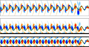
Figure 2 shows instantaneous vorticity contours at t/T = 0.75 (minimum lateral position of the leading edge; see figure 2d) in a steady state when a single fin propels with no wall (0W), near a single wall (1W) and between two parallel walls (2W), where T = 1/f is the flapping period of a fin. In general, positive (red, counter-clockwise rotation) and negative (blue, clockwise rotation) vortices are generated by downward and upward motions of the fin, respectively. An isolated fin for 0W (d/Ahead,i = ∞) generates a symmetric reverse von Kármán vortex street in figure 2(a). In figure 2(b), the presence of a single wall breaks down the symmetric nature of the wake structure, and vortices with a sign opposite to that of the main vortices form near the wall. The main positive and negative vortices generated by the flapping motion of the fin travel downstream in pairs (elliptic dashed line), and they give rise to an upward deflection caused by a vortex-induced velocity, consistent with a previous observation by Quinn et al. (Reference Quinn, Moored, Dewey and Smits2014b). However, when the fin propels between the two walls in figure 2(c), the vortex streets become nearly aligned along the centreline, maintaining their symmetric nature.
Instantaneous vorticity contours at t/T = 0.75 in a steady state when a single fin propels with (a) no wall (0W), (b) near a single wall (1W) and (c) between two parallel walls (2W). The green solid line represents the fin and the black bold solid line indicates the wall. (d) Temporal lateral position of the leading edge (Yhead) during one flapping period in a steady state; it has maximum and minimum values at t/T = 0.25 and 0.75 (vertical dashed line). (e) Instantaneous vorticity contour around a fin for 1W at t/T = 0.25. Dashed ellipses are visible in (b) to highlight pairs of vortices. The distance between the cores of the positive and negative vortices is denoted by dvor. Two consecutive vortices immediately behind the fin at the minimum Yhead (t/T = 0.75) are denoted by I and II, and those at the maximum Yhead (t/T = 0.25) are denoted by III and IV.

In order to investigate the advection of the vortices with/without wall effects, schematics of the wake structures generated by an isolated fin for 0W, 1W and 2W are presented in figure 3(a–c). Red and blue circles with arrows indicate positive and negative vortices with the direction of the rotation, respectively. In figure 3(a) for a self-propelled fin without a wall, a reverse von Kármán vortex street is observed, while the positive and negative vortices convect along the downstream direction at a constant speed (see the slope of Δxcore with respect to time in figure 3d), similar to an earlier finding by Zhu et al. (Reference Zhu, He and Zhang2014b). In figure 3(b) under a single wall, a negative vortex (2) and an induced positive vortex (2*) near the wall generate an upstream flow (toward the negative x-direction), and this pair leads to slow advection of the negative vortex (2). However, because a positive vortex (1) and an induced negative vortex (1*) on the wall accelerate the flow in the downstream direction, the positive vortex (1) tends to move faster than the negative vortex (2). As a result, the positive vortex (1) and negative vortex (2) approach each other, and thus form a vortex pair with a short distance of dvor = 1.26 (figure 2b), consistent with previous observations by Quinn et al. (Reference Quinn, Moored, Dewey and Smits2014b), Dai et al. (Reference Dai, He and Zhang2016) and Park et al. (Reference Park, Kim and Sung2017). In a vortex pair, the positive vortex is relatively strong compared to the negative one due to its formation at a later time. When the lateral position of the leading edge reaches its maximum value (t/T = 0.25), the distance between the unpaired upstream negative vortex and the downstream positive vortex is dvor = 1.93 (figure 2e). As shown in figure 3(b), ascending deflection of the wake structures (i.e. induced lateral velocity) is mostly induced by the interaction between positive and negative vortices in pairs, and the value of α is larger than that for 0W. Although the overall mechanism for the creation and advection of the vortex pairs is similar to a previous observation by Quinn et al. (Reference Quinn, Moored, Dewey and Smits2014b), the inclination angle of the deflected jet away from the wall in our study is smaller than that by Quinn et al. (Reference Quinn, Moored, Dewey and Smits2014b) due to small values of the Reynolds number and flapping frequency (i.e. Re = 100 and f = 0.398 in the present study and Re = 4700 and f = 1.280 in the study of Quinn et al. Reference Quinn, Moored, Dewey and Smits2014b). In figure 3(c) for 2W, although a downstream flow produced by positive vortex (1) and induced negative vortex (1*) near the lower wall enhances the advection speed of vortex (1), the generation of an upstream flow caused by positive vortex (1) and induced negative vortex (1**) on the upper wall cancels out the fast advection of vortex (1) (Δxcore ≈ 0 in figure 3d). Furthermore, similar opposing effects are found around vortex (2) for 2W in a downstream region. Thus, the wake structures for 2W maintain a constant distance between the vortices (dvor) without vortex pairings, and the balance between the regularly induced flows on both walls aligns the vortex wakes along the centreline at y = 0 without deflection (i.e. symmetric pattern). The small value of dvor for 2W compared to that for 0W (dvor = 1.64 for 0W and dvor = 1.42 for 2W in figure 2) stems from the weakened horizontal component of the induced flow generated between vortices (1) and (2) by the large value of α (nearly 90°).
(a–c) Schematics of the wake structures generated by an isolated fin for (a) 0W, (b) 1W and (c) 2W. Red and blue circles indicate positive and negative vortices, respectively. The orientation angle of the dipole relative to the horizontal direction is denoted by α and the distance between the positive and negative vortices is denoted by dvor. In each panel, the positive and negative vortices are denoted by 1 and 2. In (b,c), the negatively and positively induced vorticities near the lower wall are denoted by 1* and 2*, and 1** and 2** indicate the negatively and positively induced vorticities near the upper wall. Black arrows in each panel indicate the induced velocities. (d) Time history of the moving distance for the vortex (1) core (Δxcore) during 0.75 ≤ t/T < 1.4. Circle, 0W; triangle, 1W; square, 2W. A positive vortex immediately behind the fin (i.e. vortex (1)) is formed at t/T = 0.75 in figure 2, and it travels downstream with time due to the horizontal component of the induced flow generated between vortices (1) and (2).

Figure 4 shows the instantaneous horizontal (u) and lateral velocity (v) contours around a fin at t/T = 0.75 in a steady state for 0W, 1W and 2W. Solid and dashed lines correspondingly indicate contour levels of u = 0.9 and −0.9 and v = 1.1 and −1.1 to highlight the strong velocity components. The jet-like flows of positive horizontal velocity immediately behind the fins for 1W and 2W are stronger than that for 0W (see the solid lines), as most of the momentum generated by the downward motion of the fin is transferred to the horizontal direction due to the presence of the walls. Because figure 4(a) presents one instantaneous plot over one cycle, we estimate time-averaged values of an effective positive horizontal velocity around fins for 0W, 1W and 2W during one flapping period to provide further evidence for the increase of the jet-like flows behind the fins for 1W and 2W. The time averaging is conducted using data within a rectangular box (see the box in figure 4a), and this box size (Xhead + 1.0 ≤ x ≤ Xhead + 2.2 and Yhead − 0.45 ≤ y ≤ Yhead + 0.45) is determined with respect to the fixed position of the leading edge (Xhead, Yhead) of a fin. This procedure is required to avoid overestimation by non-effective positive horizontal flow near the leading edge (i.e. positive horizontal velocities above and under a fin). The results show that the time-averaged values of the positive horizontal velocity behind the fins are 0.447 and 0.471 for 1W and 2W, which are larger than a value of 0.378 for 0W.
(a,b) Instantaneous (a) horizontal velocity (u) and (b) lateral velocity (v) contours around a fin at t/T = 0.75 in a steady state for (i) 0W, (ii) 1W and (iii) 2W. In (a), the rectangular boxes (Xhead + 1.0 ≤ x ≤ Xhead + 2.2 and Yhead − 0.45 ≤ y ≤ Yhead + 0.45) are depicted to estimate time-averaged values of the horizontal velocity component generated behind the fins. Solid and dashed lines indicate the contour levels of u = 0.9 and −0.9 and v = 1.1 and −1.1, respectively.

In figure 4(b), an alternating sign of the positive and negative lateral flows is clearly observed behind the propelling fins. In figure 4(b-ii), a strong positive lateral flow is found behind the fin for 1W compared to that for 0W. For the fin for 2W in figure 4(b-iii), a strong positive lateral flow persists downstream, consistent with the observation for 1W. Because it has been reported that the follower in a tandem configuration takes an energetic benefit by utilizing the lateral flow generated by the leader (Zhu et al. Reference Zhu, He and Zhang2014a), it is important to examine why the strength of the lateral flow is increased by the wall effect. To explain the increased lateral flow strength generated by an isolated fin in detail, vortices I, II, III and IV shown in figure 2 are analysed based on the vortex dipole model suggested by Godoy-Diana et al. (Reference Godoy-Diana, Marais, Aider and Wesfreid2009). According to the vortex dipole model (figure 5), the lateral component of the dipole-induced velocity is estimated by  ${v_\varGamma } = (\varGamma /2{\rm \pi} {d_{vor}})\sin \alpha$, where Γ is the average circulation of the two vortices in the dipole (Zheng & Wei Reference Zheng and Wei2012). The circulation of the vortex is calculated by integrating the vorticity over a rectangular area, which is determined by performing Gaussian fits,
 ${\textrm{e}^{( - x_i^2/\sigma _i^2)}}$, along the x- and y-directions with respect to the positions of the vorticity maxima and minima. The size of the vortex along the x- and y-directions is defined as 2σi (Godoy-Diana et al. Reference Godoy-Diana, Marais, Aider and Wesfreid2009; Zheng & Wei Reference Zheng and Wei2012). For the two dipoles (I, II) and (III, IV), the estimated values of the circulation (Γ), distance between the vortex cores (dvor), orientation angle (α) and strength of the lateral flow (
 ${v_\varGamma }$) are tabulated in figure 5. Because the induced flow in the horizontal direction by the interaction between the main vortex and induced vortex near the wall (for example, see the induced flow generated between negative vortex (2) and induced positive vortex (2*) in figure 3b) enhances further the circulation of the main vortices (Zhang et al. Reference Zhang, Huang and Lu2017), the estimated values of Γ 1 and Γ 2 for 1W and 2W are greater than those for 0W. The enhanced circulations with a large value of α and a small value of dvor lead to a large magnitude of the lateral velocity (
 ${v_\varGamma }$) for 1W and 2W, although the magnitude of
 ${v_{\varGamma ,2}}$ for 1W is similar to that for 0W due to the large value of dvor 2. The large magnitude of Γ 2 for 1W compared to the value of Γ 1 is a direct influence of a strong induced flow by the wall (see vortex III).
Schematic of the vortex dipoles formed between vortices I and II and between vortices III and IV (figure 2). Values of the circulation (Γ), distance between the vortex cores (dvor), orientation angle (α) and strength of the lateral flow ( ${v_\varGamma }$) for the two dipoles (I, II) and (III, IV) are tabulated in the table. Here, the subscripts 1 and 2 represent values formed between vortices I and II and between vortices III and IV, respectively.

3.2. Fluid-mediated interactions in tandem configurations
In this section, fluid-mediated interactions between two self-propelled tandem flexible fins for 0W, 1W and 2W are analysed to reveal the change of the flapping modes for efficient propulsion of the follower with wall effects. The distances between the fin and the wall are d/Ahead,l = ∞ for 0W and 2.5 for 1W and 2W. In addition, we set the following values: Ahead,l = Ahead,f = 0.4, ϕ = 0 and γ = 1.0. The simulations of the tandem fins for 0W, 1W and 2W start with an initial gap distance of (1 ≤ Gx,o ≤ 9) at t/T = 0, and the fins approach equilibrium states after any transient effect.
3.2.1. Emergent configurations and dynamics
In order to show the formation of the emergent sparse configurations for 0W, 1W and 2W, the variations of the horizontal gap distance between the leader and follower (Gx) and the average horizontal speed (Uavg) of the fins as a function of time for 0W, 1W and 2W are presented in figure 6. The average horizontal speed of a fin is defined as  ${U_{avg}} = \int_0^1 {|\partial X(s,t)/\partial t|\,\textrm{d}s}$. In figure 6(a,c,e), the three stable tandem configurations form spontaneously between the leader and follower regardless of the external conditions (0W, 1W and 2W). It is again noted that, with the present parameter settings, only a sparse configuration is observed, whereas a compact configuration could be observed through the manipulation of other parameters (γ, ϕ, Ahead,l and Ahead,f) (Zhu et al. Reference Zhu, He and Zhang2014a; Lin et al. Reference Lin, Wu, Zhang and Yang2020). The discrete equilibrium horizontal gap distances (Gx,eq 1, Gx,eq 2 and Gx,eq 3) for 0W, 1W and 2W are determined dynamically depending on the initial horizontal gap distance (Gx,o). However, each value of Gx,eq 1, Gx,eq 2 and Gx,eq 3 is affected by the external environments (0W, 1W and 2W). For example, the first equilibrium horizontal gap distances (Gx,eq 1) for 0W, 1W and 2W are achieved within seven flapping periods from the start (t/T = 0), and the values of Gx,eq 1 for 0W, 1W and 2W are 2.59, 2.34 and 2.07, respectively. Although the value of Gx,eq 1 is determined by the wavelength of motion
 $(\lambda = \overline {{U_{avg}}} /f)$ and the advection speed of the vortices, the smaller values of Gx,eq 1 for 1W and 2W than that for 0W mainly stem from the reduction of the advection velocity, as shown in figure 3(d). Here, the cruising speed during one flapping cycle in a steady state is defined as
 $\overline {{U_{avg}}} = (1/T)\int_0^T {{U_{avg}}\,\textrm{d}t}$ (the overbar indicates the time-average value during one cycle).
(a,c,e) Temporal variations of the horizontal gap distance between two tandem fins (Gx) and (b,d,f) temporal variation of the average horizontal speed (Uavg) for fins at Gx,eq 1 with Gx,o = 1.0 and Gx,o = 3.0: (a,b) 0W, (c,d) 1W and (e,f) 2W. The horizontal position of the leading edge for the leader is initially prescribed at x = 21.0, and that for the follower is positioned downstream with an initial gap distance (Gx,o). The blue and green lines represent values of Gx,o = 1.0 and Gx,o = 3.0, respectively.

In figures 6(a) and 6(e), the difference between the discrete equilibrium gap distances (i.e. Gx,eq 2 − Gx,eq 1 or Gx,eq 3 − Gx,eq 2) is nearly constant (approximately 3.12 or 3.14) for 0W and 2W, corresponding to the horizontal spatial period of the vortex street (Zhu et al. Reference Zhu, He and Zhang2014a). The slightly larger difference of the fins for 2W results from the higher  $\overline {{U_{avg}}}$ of the fins in figures 6(b) and 6(f). However, the interval between the discrete equilibrium gap distances is not constant for 1W (i.e. Gx,eq 2 − Gx,eq 1 = 3.27 and Gx,eq 3 − Gx,eq 2 = 3.14). Because advection of the vortices is delayed due to the strong effects of the upstream flow for a small Gx,eq (figure 2), the value of Gx,eq 1 decreases, leading to a large value of Gx,eq 2 − Gx,eq 1. However, the ascending motion of the vortex pairs with an increase in Gx,eq weakens the effects of the upstream flow induced by the main negative vortex and the induced positive vortex (figure 2), making the value of Gx,eq 3 − Gx,eq 2 similar to that for 0W or 2W.
In figure 6(b,d,f) with Gx,o = 1.0 (blue) and 3.0 (green), the trajectory of Uavg for the leader and follower is nearly identical before the follower encounters the vortices generated by the leader (t/T < 0.9). However, the magnitude of Uavg for the follower increases (green; Gx,o = 3.0) or decreases (blue; Gx,o = 1.0) dramatically in the transient state (1 < t/T < 7) for the follower to reach the equilibrium gap distance (Gx,eq 1), compared to that for the leader (or an isolated fin) (red). In the steady state (t/T > 7.0), the time-averaged horizontal speed  $(\overline {{U_{avg}}} )$ of the fins for 1W and 2W is higher than that of the fin for 0W (
 $\overline {{U_{avg}}} = 1.12$, 1.14 and 1.20 for 0W, 1W and 2W), and the magnitude of
 $\overline {{U_{avg}}}$ for the follower is similar to that for the leader in each case.
Because the pattern of vortex–body interactions is crucial for understanding the propulsive performance of the follower in the tandem configuration (Liao et al. Reference Liao, Beal, Lauder and Triantafyllou2003; Jia & Yin Reference Jia and Yin2008; Zhu et al. Reference Zhu, He and Zhang2014a; Uddin et al. Reference Uddin, Huang and Sung2015; Peng et al. Reference Peng, Huang and Lu2018b,Reference Peng, Huang and Luc), the time evolution of the vorticity along the lateral line at the leading edge of the follower at Gx,eq 1 for 0W, 1W and 2W is plotted in figure 7. The direction of the time evolution is leftward, identical to the moving direction of the fins. In figure 7(a), the leading edge of the follower for 0W interacts with the oncoming vortices generated by the leader swimming near the vortex cores, i.e. the vortex interception mode, consistent with an earlier observation by Zhu et al. (Reference Zhu, He and Zhang2014a). Interestingly, the leading edge trajectory of the follower for 1W in figure 7(b) is locked onto only positive vortex cores, and the leading edge of the fin moves forward by slaloming between the negative vortex and the wall (i.e. a combination of the vortex interception mode and slalom mode, hereafter, the ‘mixed mode’). In figure 7(c), the leading edge of the following fin for 2W propels forward by slaloming between positive and negative vortices shed from the leader, instead of passing through the vortex cores. This slalom mode has only been observed for a passively or actively flapping fin behind a tethered flapping flexible or rigid body in a uniform flow to reduce the energy required by the upstream drag wake (Liao et al. Reference Liao, Beal, Lauder and Triantafyllou2003; Jia & Yin Reference Jia and Yin2008; Uddin et al. Reference Uddin, Huang and Sung2015). Although not shown, the vortex–body interaction shown in figure 7 for each case is not affected by the value of Gx,eq, similar to previous observations for two self-propelled tandem fins in the sparse configuration (Zhu et al. Reference Zhu, He and Zhang2014a; Park & Sung Reference Park and Sung2018).
Time evolution of the vorticity along the lateral line at the leading edge of the follower at the first equilibrium gap distance (Gx,eq 1) for (a) 0W, (b) 1W and (c) 2W. The green line denotes the leading edge trajectory of the follower. The initial horizontal gap distance is Gx,o = 2.0.

Figure 8 shows time evolution of the horizontal (u) and the wall-normal (v) velocity along the lateral line at the leading edge of the follower for 0W, 1W and 2W. Solid and dashed lines indicate contour levels of 1.1 and −1.1 to highlight strong lateral velocity. In figure 8(a-i), the leading edge of the follower for 0W encounters the jet-like flow consistently during all flapping periods (except at the maximum and minimum lateral positions). In figure 8(a-ii), the leading edge of the following fin for 1W faces the negative horizontal velocity during its upward motion. However, when the leading edge of the follower is in a downward motion, it encounters a strong positive horizontal velocity. For the follower for 2W in figure 8(a-iii), the leading edge trajectory encounters only the negative horizontal flow near the walls. In figure 8(b), the leading edge of the follower for 0W, 1W and 2W passes through the positive and negative lateral flows alternatively during the upward and downward motions of the leading edge, indicating that the lateral motion of the leading edge for the follower is in phase with the induced lateral flow by the leader. The strength of the lateral flow acting on the leading edge of the follower for 1W and 2W is greater than that for 0W in figure 8(b) (see the solid and dashed lines), consistent with our observations in figure 5. However, it should be noted that the magnitude of the negative lateral flow for 1W is similar to that for 0W.
Time evolution of (a) the horizontal (u) and (b) lateral (v) velocity along the lateral line at the leading edge of the follower at the first equilibrium gap distance (Gx,eq 1) for (i) 0W, (ii) 1W and (iii) 2W. The green line denotes the leading edge trajectory of the follower. In (b), solid and dashed lines indicate contour levels of 1.1 and −1.1, respectively.

To examine the influence of fluid-mediated interactions on the propulsive performance of the follower, the time histories of the leading and trailing edge lateral positions (Y), the average lateral velocity (Vavg) of the fin, the lateral component of the temporal input power (Py) and the average lateral flow (vavg) acting on the follower during one flapping period are presented in figure 9. The average lateral velocity (Vavg) of a fin is defined as  ${V_{avg}} = \int_0^1 {(\partial Y(s,t)/\partial t)\,\textrm{d}s}$, indicating an average velocity of a flexible fin. The average lateral flow (vavg) acting on the follower is analysed due to its direct influence on the input power of the follower, and it is defined as
 ${v_{avg}} = \int_0^1 {({v_f}(s,t) - {v_i}(s,t))\,\textrm{d}s}$, indicating an average velocity of the fluid around the follower (where vf and vi denote the lateral flow acting on the follower and an isolated fin, respectively). Because a lateral flow is also induced by the active motion of the fin itself in figure 4, the subtraction of vi generated by an isolated fin is required to estimate the pure benefit from the lateral flow (generated by the leader) around the follower. The temporal input power to produce the flapping motion of a fin is calculated using the lateral component of the force and velocity acting on the fin, i.e.
 ${P_y} = \int_0^1 {({F_{L,y}}(\partial Y/\partial t))\,\textrm{d}s}$, where FL,y is the lateral component of the Lagrangian force. For a self-propelled fin, the time-averaged horizontal force acting on the fin over the cycle is zero (Ramananarivo et al. Reference Ramananarivo, Fang, Oza, Zhang and Ristroph2016; Peng et al. Reference Peng, Huang and Lu2018a,Reference Peng, Huang and Lub,Reference Peng, Huang and Luc), and the horizontal moving speed is nearly constant in the steady state, as shown in figure 6(b,d,f). Thus, the horizontal component of the time-averaged input power
 $(\int_0^1 {({F_{L,x}}(\partial X/\partial t))\,\textrm{d}s} )$ in the steady state is zero. Because the time-averaged input power (Pin) of the follower in the sparse configuration reduces with a decrease of the equilibrium horizontal gap distance (Gx,eq) (Park & Sung Reference Park and Sung2018), we here consider the smallest equilibrium gap distance (i.e. Gx,eq 1 in figure 6), where the time-averaged input power in the steady state is estimated via
 ${P_{in}} = (1/T)\int_0^T {{P_y}\,\textrm{d}t}$. In addition, time reference in a steady state is newly defined hereafter by setting the start of the 11th cycle (figure 6) to t/T = 0.
Time histories of the (a–c) leading and trailing edge lateral positions (Y), (d–f) the average lateral velocity (Vavg), (g–i) the lateral component of the temporal input power (Py) and (j–l) the average lateral flow (vavg) acting on the follower during one flapping period at the first equilibrium gap distance (Gx,eq 1). (m–o) Superimposition of the leading edge trajectory for the follower onto instantaneous vorticity contours generated by an isolated fin. Vertical dashed lines in (m–o) indicate the horizontal positions of the vortex cores. (a,d,g,j,m) 0W, (b,e,h,k,n) 1W and (c,f,i,l,o) 2W.

In figure 9(a), the flapping of the leader (red) and follower (blue) for 0W is symmetric with respect to the centreline, consistent with the wake patterns in figure 2(a). The peak-to-peak amplitude of the trailing edge (Atail) of the follower for 0W is larger than that of the leader, similar to previous observations of a self-propelled two-fin system in tandem and staggered configurations without a wall (Park & Sung Reference Park and Sung2018; Peng et al. Reference Peng, Huang and Lu2018a). The magnitude of the average lateral velocity (Vavg) of the follower for 0W increases in figure 9(d) due to the intensification of Atail, and the increased Vavg of the follower leads to an increase of Py in the ranges of 0.0 < t/T < 0.05, 0.45 < t/T < 0.55 and 0.95 < t/T < 1.0 in figure 9(g). Despite the penalty on Py due to the enhanced flapping amplitude for the follower, the time-averaged value of Py (i.e. Pin) for the follower reduces by up to 5.3 % compared to that of the leader owing to the synchronized lateral flow (figure 8b), consistent with earlier findings for two self-propelled tandem fins in the sparse configuration without a wall (Zhu et al. Reference Zhu, He and Zhang2014a; Park & Sung Reference Park and Sung2018). More specifically, the average lateral flow (vavg) acting on the whole body of the follower in figure 9(j) demonstrates that the synchronized body motion of the follower (figure 9d) with the strong lateral flow (figure 9j) in the range of 0.05 < t/T < 0.25 and 0.55 < t/T < 0.75 leads to a large reduction of Py for the follower in figure 9(g). However, the signs of vavg and Vavg are opposite approximately in the ranges of 0.3 < t/T < 0.45 and 0.8 < t/T < 0.95. This anti-phase behaviour for 0W is observed through the time evolution of the lateral velocity immediately after the maximum and minimum lateral positions in figure 8(b-i), where the lateral motion of the leading edge for the follower is temporarily in anti-phase with the lateral flow. Furthermore, visualization of the instantaneous vorticity contour generated by an isolated fin with superposition of the leading edge trajectory for the follower in figure 9(m) more clearly shows anti-phase behaviour, leading to an increase in Py for the follower.
For the fins for 1W in figure 9(b), asymmetric flapping arises with the corresponding asymmetric wake pattern shown in figure 2(b). When the follower is in a downward motion (0.45 < t/T < 0.6), the increased Vavg of the follower in figure 9(e) compared to the leader due to large Atail (figure 9b) results in the large magnitude of Py in figure 9(h). In addition, the large magnitude of Py for the follower in the range of 0.8 < t/T < 0.95 is attributed to the anti-synchronization between Vavg and vavg in figures 9(e) and 9(k). Similar to the observation for 0W, the lateral motion of the leading edge for the follower is temporarily in anti-phase with the lateral flow near the minimum lateral position (figure 8b-ii), as the horizontal position of the negative vortex deviates from that for the minimum lateral position of the follower (figure 9n). However, because the horizontal position of the positive vortex is collapsed with that for the maximum lateral position of the follower, there is no penalty of Py from the anti-phase motion in the range of 0.3 < t/T < 0.45 in figure 9(h). When the follower encounters the strong positive lateral velocity by a vortex pair during the upward motion (0.0 < t/T < 0.3), the magnitude of Py for the follower decreases significantly in figure 9(h) despite the large magnitude of Vavg. As a result, the value of Pin of the follower is smaller by approximately 11.4 % that of the leader.
In figure 9(c) for 2W, symmetric flapping for the leader and follower is observed, consistent with the wake pattern in figure 2(c). The value of Atail of the leader for 2W is 1.43, which is smaller than that for 0W and 1W due to influence of the sidewalls (Atail = 1.51 for 0W and Atail = 1.47 for 1W). Contrary to the observation for 0W and 1W, the signs of Vavg and vavg for 2W are always identical during the flapping period in figures 9(f) and 9(l) due to the coincidence of the horizontal positions for the vortex cores and those of the maximum and minimum lateral positions of the follower (figure 9o) (also see figure 7c and figure 8b-iii). Although the value of Vavg for the follower increases compared to that for the leader in figure 9(f), the consistent benefit from the strong lateral flow in figure 9(l) without anti-synchronization between Vavg and vavg dominantly decreases the value of Py for the follower over most flapping periods in figure 9(i). The value of Pin for the follower decreases by approximately 18.7 % compared to that for the leader.
3.2.2. Pressure distributions with force decomposition
In an effort to reveal not only how the synchronized lateral flow reduces the input power of the follower but also how the follower utilizes the induced horizontal flow in the moving direction, we investigate the pressure distributions around two fins with force decomposition. For a quantitative analysis of the hydrodynamic forces with/without wall effects, the force at a certain Lagrangian point (FL) is decomposed into the normal  $(\boldsymbol{F}_L^n)$ and tangential
 $(\boldsymbol{F}_L^\tau )$ forces, as shown in figure 10. The normal force is mainly determined by the pressure difference between the upper and lower areas of the fin, while the tangential force originates from the viscosity of the fluid
 \begin{gather}{\boldsymbol{F}_L} = [ - p{\boldsymbol{\mathsf{I}}_L} + {\boldsymbol{\mathsf{T}}_L}]\boldsymbol{\cdot }\boldsymbol{n} = \boldsymbol{F}_L^n + \boldsymbol{F}_L^\tau ,\end{gather}
 \begin{gather}\boldsymbol{F}_L^n\boldsymbol{= }\textrm{(}{\boldsymbol{F}_L}\boldsymbol{\cdot }\boldsymbol{n}\textrm{)}\boldsymbol{n} = \textrm{(}F_{L,x}^n, F_{L,y}^n\textrm{),}\end{gather}
 \begin{gather}\boldsymbol{F}_L^\tau \boldsymbol{= }\textrm{(}{\boldsymbol{F}_L}\boldsymbol{\cdot }\boldsymbol{\tau }\textrm{)}\boldsymbol{\tau } = \textrm{(}F_{L,x}^\tau , F_{L,y}^\tau \textrm{),}\end{gather}
where  $\boldsymbol{\mathsf{I}}_{L}$ is the unit tensor,
 $\boldsymbol{\mathsf{T}}_{L}$ is the viscous stress tensor, n and τ are the unit normal and tangential vector, respectively, and [
 $-p\boldsymbol{\mathsf{I}}_{L}+\boldsymbol{\mathsf{T}}_{L}$] in (3.1) represents the quantitative variation of the normal and tangential stresses across the immersed boundary (Peng et al. Reference Peng, Huang and Lu2018a; Huang & Tian Reference Huang and Tian2019). The horizontal normal and tangential forces (
 $F_x^n$ and
 $F_x^\tau$) and the lateral normal and tangential forces (
 $F_y^n$ and
 $F_y^\tau$) are calculated respectively using the integrals of
 $F_{L,x}^n$ and
 $F_{L,y}^n$ and
 $F_{L,x}^\tau$ and
 $F_{L,y}^\tau$ along the fin (figure 10)
 \begin{gather}F_x^n\boldsymbol{= }\int_0^1 {F_{L,x}^n} \,\textrm{d}s,\quad F_y^n\boldsymbol{= }\int_0^1 {F_{L,y}^n} \,\textrm{d}s,\end{gather}
 \begin{gather}F_x^\tau \boldsymbol{= }\int_0^1 {F_{L,x}^\tau } \,\textrm{d}s,\quad F_y^\tau \boldsymbol{= }\int_0^1 {F_{L,y}^\tau } \,\textrm{d}s.\end{gather}
For a self-propelled fin, the horizontal normal force  $(F_x^n)$ induced by the active flapping motion is generally negative, and the negative
 $F_x^n$ contributes to the generation of thrust force (forward propulsion) toward the negative x-direction (Thiria & Godoy-Diana Reference Thiria and Godoy-Diana2010; Ramananarivo, Godoy-Diana & Thiria Reference Ramananarivo, Godoy-Diana and Thiria2011; Peng et al. Reference Peng, Huang and Lu2018a). However, even when the value of
 $F_x^n$ is negative, the horizontal resultant force (Fx) acting on the fin can be positive (i.e. drag force acting in the positive x-direction) due to the strongly positive drag-related horizontal tangential force
 $(F_x^\tau )$ by viscosity.
Schematic of a flexible fin during the downward motion for the force decomposition. The force at a certain Lagrangian point (FL) is decomposed into the normal ( $\boldsymbol{F}_L^n$) and tangential (
 $\boldsymbol{F}_L^\tau$) forces;
 $F_{L,x}^n$ and
 $F_{L,y}^n$ denote the horizontal and lateral normal forces, and
 $F_{L,x}^\tau$ and
 $F_{L,y}^\tau$ denote the horizontal and lateral tangential forces. Blue line indicates the fin. n and τ indicate the local normal and tangential vectors, respectively. θL represents the local slope at a certain point of the fin.

The instantaneous pressure contours for 0W using the data in figure 9 are visualized during a half-flapping period (0.0 ≤ t/T ≤ 0.5) in figure 11(a). As shown in figure 9, the hydrodynamic behaviours around the fins for 0.5 ≤ t/T ≤ 1.0 are symmetric to those for 0.0 ≤ t/T ≤ 0.5 with respect to the centreline (y = 0). At t/T = 0.125, the pressure difference between the upper and lower sides of the follower is smaller than that of the leader in figure 11(a-i), leading to a reduction of  $F_x^n$ acting on the follower (figure 11b). When the leading edges of the fins are located at the maximum lateral position (t/T = 0.25) in figure 11(a-ii),
 $F_x^n$ for the leader and follower is oriented toward the downstream direction (i.e. the drag force in figure 11b). At t/T = 0.125 and 0.25 (during the upward motion in figure 9a), the absolute magnitude of
 $F_y^n$ for the follower is significantly low compared to that of the leader in figure 11(c) due to the reduction of the pressure difference across the follower. The decreased pressure difference across the follower can be explained by the flow-mediated interactions because the flow resistance that interferes with the active motion of the follower is reduced with the help of the synchronized lateral flow (figure 8b). The reduced pressure difference leads to the decrease of the temporal input power (Py) for the follower in figure 9(g) despite the increased flapping amplitude (figure 9d). At t/T = 0.375 and 0.5 (during the downward motion in figure 9a), the pressure on the upper area of the follower is lower than that of the leader due to the influence of vortex-induced negative pressure in front of the follower at t/T = 0.25 (see figure 11a-ii), generating a larger amount of thrust force (figure 11b). In addition, the large magnitude of the negative pressure contours at t/T = 0.5 can be partially attributed to the large lateral velocity of the follower in figure 9(d), indicating that the increased tail amplitude of the follower due to the vortex–body interaction contributes to the enhancement of the thrust force. However, the magnitude of
 $F_y^n$ for the follower at t/T = 0.375 is slightly larger than that for the leader (figure 11c), resulting in a slight increase of Py in figure 9(g). The lateral normal force
 $(F_y^n)$ of the follower at t/T = 0.5 is similar to that of the leader in figure 11(c).
(a) Instantaneous pressure contours around two fins during a half flapping period for 0W at (i) t/T = 0.125, (ii) t/T = 0.25, (iii) t/T = 0.375 and (iv) t/T = 0.5. In (a), solid and dashed lines indicate the positive and negative pressure contours with an interval of 0.16, respectively. (b) Horizontal normal force ( $F_x^n$), (c) lateral normal force (
 $F_y^n$), (d) horizontal tangential force (
 $F_x^\tau$) and (e) lateral tangential force (
 $F_y^\tau$) experienced by the fins for 0W during one heaving period. In (b–e), the four instances (i–iv) observed in (a) are indicated by the vertical dashed lines.

In figure 11(d), variation of the horizontal tangential force  $(F_x^\tau )$ shows that the drag generated by the fluid viscosity is always acting on the leader and follower during the entire flapping period. It is noted that the sum of the time-averaged
 $F_x^n$ and
 $F_x^\tau$ in figures 11(b) and 11(d) is zero. The magnitude of
 $F_x^\tau$ for the follower is larger than that for the leader (i.e. large drag force acting on the follower) due to an interruption of the jet-like flow (figure 8a), similar to previous observations of two self-propelled tandem fins (Park & Sung Reference Park and Sung2018; Lin et al. Reference Lin, Wu, Zhang and Yang2019). To overcome the increased drag force, a large value of
 $F_x^n$ for the follower (figure 11b) is required for the generation of thrust. Such a large amount of thrust for the follower is induced by the vortex-induced negative pressure acting on the follower at t/T = 0.375 and 0.5. In order to utilize the negative pressure to generate strong thrust for a long period, the follower at t/T = 0.25 should be positioned near the rear part of the vortex core when it is at the maximum lateral position (i.e. anti-phase motion in figure 9m). When the follower moves downward in the range of 0.25 < t/T ≤ 0.5, the vortex-induced negative pressure influences the pressure on the upper side of the follower (at t/T = 0.375 and 0.5), and the large pressure difference across the flexible fin in the horizontal direction generates a large amount of thrust force, similar to previous observations of two tethered tandem heaving and pitching foils in a uniform flow (Boschitsch et al. Reference Boschitsch, Dewey and Smits2014; Muscutt, Weymouth & Ganapathisubramani Reference Muscutt, Weymouth and Ganapathisubramani2017). In figure 11(e), the absolute magnitude of
 $F_y^\tau$ for the follower is greater than that that of the leader due to the dominant influence of the intensified flapping amplitude. However, the value of
 $F_y^\tau$ is much smaller than that of
 $F_y^n$; thus, the lateral force (Fy) acting on the fins is mainly determined by
 $F_y^n$.
The instantaneous pressure contours around two fins during one flapping period (0.0 ≤ t/T ≤ 1.0) for 1W are shown in figure 12(a). Contrary to the observations for 0W in figure 11, asymmetric pressure distributions with respect to the mean lateral position of the leading edge (y = 1.0) are evident. When the follower experiences a strong synchronized lateral flow due to the ascending vortex pair at t/T = 0.125 and 0.25 (during the upward motion in figure 9b) in figure 9(k), the pressure difference across the fin is significantly reduced in figures 12(a-i) and 12(a-ii). At t/T = 0.125, the reduction of the pressure difference across the follower leads to lower magnitudes of  $F_x^n$ and
 $F_y^n$ compared to those for the leader in figures 12(b) and 12(c). At t/T = 0.25, the positive
 $F_x^n$ (drag force) is acting on the leader in figure 12(b). The decrease of
 $F_y^n$ in figure 12(c) results in a reduction of Py for the follower at t/T = 0.125 and 0.25 in figure 9(h). Contrary to the trajectory of the follower for 0W, the follower for 1W at t/T = 0.25 encounters the vortex-induced negative pressure without the anti-phase motion in figure 12(a-ii), consistent with our observations in figures 7(b) and 9(n). At t/T = 0.25, both the upper and lower sides of the follower are affected by the vortex-induced negative pressure, and the value of
 $F_x^n$ for the follower is nearly zero. At t/T = 0.375, negative pressure of a large magnitude is induced below the follower by the strong positive horizontal flow (see figure 8a-ii) with a nearly zero average lateral flow (vavg) acting on the follower in figure 9(k). However, the emergence of negative pressure above the follower near the trailing edge results in a low magnitude of the negative
 $F_x^n$ for the follower. At t/T = 0.5, the large magnitude of the negative pressure contours above the follower is attributed to the large lateral velocity of the follower in figure 9(e), leading to an enhancement of the thrust force (i.e. increase of
 $F_x^n$). The magnitude of
 $F_y^n$ for the follower at t/T = 0.375 and 0.5 is similar to that of the leader in figure 12(c).
Identical to figure 11 but pertaining to contours around two fins during one flapping period for 1W at (i) t/T = 0.125, (ii) t/T = 0.25, (iii) t/T = 0.375, (iv) t/T = 0.5, (v) t/T = 0.625, (vi) t/T = 0.75, (vii) t/T = 0.875 and (viii) t/T = 1.0. In (b–e), the eight instances (i–viii) observed in (a) are denoted by the vertical dashed lines.

When the fin approaches the wall at t/T = 0.625, strong positive pressure contours are induced under the fin due to the presence of the wall. The value of  $F_x^n$ for the follower is lower than that of the leader due to the small deformation at this point. The difference in
 $F_y^n$ between the leader and follower is small compared to that at t/T = 0.125 during the upward motion due to the weak synchronized lateral flow in figure 9(k). At t/T = 0.75, drag forces
 $(F_x^n \gt 0)$ acting on the fins (figure 12b) are induced by the pressure difference across the fins in figure 12(a-vi). In addition, a small pressure difference around the follower leads to the low magnitude of
 $F_y^n$ in figure 12(c). Because the follower experiences a relatively weak lateral flow during the downward motion (0.5 ≤ t/T ≤ 0.75) in figure 9(k), the pressure difference across the follower at t/T = 0.5, 0.625 and 0.75 is larger than that at t/T = 0.125 and 0.25. When the average lateral flow (vavg) acting on the follower is weak at t/T = 0.875 in figure 9(k), negative pressure of a large magnitude below the follower in figure 12(a-vii) is induced by the strong negative horizontal flow under the follower (figure 8a-ii), resulting in an increase of the magnitudes of
 $F_x^n$ and
 $F_y^n$ in figures 12(b) and 12(c). Although the value of
 $F_x^n$ for the follower at t/T = 1.0 is similar to that for the leader in figure 12(b), the positive pressure contours created above the leading edge of the leader in figure 12(a-viii) lead to the large magnitude of
 $F_y^n$ for the leader in figure 12(c). In figure 12(d), when the follower is in the downward motion (0.25 ≤ t/T ≤ 0.8), the magnitude of
 $F_x^\tau$ for the follower is greater than that for the leader due to the hindrance of the positive horizontal flow in figure 8(a-ii). The slightly lower
 $F_x^\tau$ for the follower during the upward motion (0.8 ≤ t/T ≤ 1.0) stems from the negative horizontal flow (figure 8a-ii). In figure 12(e), the magnitude of
 $F_y^\tau$ for the follower is larger than that that of the leader, consistent with the observation for 0W (figure 11e).
The instantaneous pressure contours around two fins during the half-flapping period (0.0 ≤ t/T ≤ 0.5) for 2W are visualized in figure 13(a). When the follower experiences a synchronized lateral flow during the upward motion at t/T = 0.125 and 0.25 in figure 9(l), the pressure difference across the follower is reduced compared to the leader in figures 13(a-i) and 13(a-ii). For the follower at t/T = 0.125, the smaller pressure difference across the follower leads to a reduction of  $F_x^n$ and
 $F_y^n$ compared to the leader in figures 13(b) and 13(c). Because the pressure decreases across the flexible fin toward the downstream direction at t/T = 0.25, the fins experience a drag force in figure 13(b). The reduction of
 $F_y^n$ for the follower at t/T = 0.125 and 0.25 by the lateral flow leads to a decrease of Py for the follower, as shown in figure 9(i). When the trailing edge of the follower is at the maximum lateral position at t/T = 0.375, negative pressure of a large magnitude above the follower near the trailing edge induced by the strong negative horizontal flow above the follower (figure 8a-iii) helps the follower increase its thrust (figure 13b). The value of
 $F_x^n$ for the follower is similar to that for the leader at t/T = 0.5. However, the value of
 $F_y^n$ for the follower is lower than that for the leader due to the synchronized lateral flow in figure 9(l). Although not shown,
 $|\overline {F_x^n} |$ of the follower over one flapping period is approximately 14 % lower than that of the leader. Because the follower for 2W utilizes a negative horizontal flow in figure 8(a-iii), the reduction of
 $F_x^\tau$ in figure 13(d) leads to the low thrust force for the follower shown in figure 13(b) to maintain the equilibrium gap distance in a stable configuration. The difference in
 $F_y^\tau$ between the leader and follower is relatively small in figure 13(e).
Identical to figure 11, but for contours around two fins during a half flapping period for 2W at (i) t/T = 0.125, (ii) t/T = 0.25, (iii) t/T = 0.375 and (iv) t/T = 0.5. In (b–e), the four instances (i–iv) observed in (a) are indicated by the vertical dashed lines.

In the present study, the propulsive performance (i.e. input power and drag/thrust forces) of the follower in a sparse configuration is a direct consequence of flow-mediated interactions. In order to maintain a stable configuration, the followers for 0W and 1W require a 30 % and 12.9 % greater thrust force (based on the absolute value of the time-averaged horizontal normal force,  $|\overline {F_x^n} |$), compared to that of the leader due to the influence of the jet-like flow. However, the thrust force generated by the follower for 2W is lower by 14 % than that of the leader due to the help of the negative horizontal flow. When the follower passes close to the vortex core (i.e. the vortex interception mode), a large amount of thrust is induced by the influence of the vortex-induced negative pressure. In addition, anti-phase motion for 0W is essential to generate a large amount of thrust for a long period, as shown in figure 11, despite the penalty for the input power. Compared to the trajectory of the follower for 0W, the follower for 1W passes through the vortex core at the maximum lateral position without anti-phase motion to maximize the benefit from the lateral flow, and thus the thrust force acting on the follower for 1W is smaller than that for 0W. However, the follower for 1W can maintain the schooling formation due to the help of the negative horizontal flow. As shown in figure 13(b), the slalom mode employed by the follower for 2W does not generate a large amount of thrust force due to the absence of a jet-like flow. However, adopting the slalom mode for 2W enhances the energetic benefit from the lateral flow to minimize the time-averaged input power. Because the stronger synchronized lateral flow under the influence of the walls in figure 8(b) greatly reduces the pressure difference across the follower for 1W and 2W compared to that for 0W in figures 11–13, time averaging of the absolute lateral normal force (i.e.
 $|\overline {F_y^n} |$) of the followers for 0W, 1W and 2W results in reductions of approximately 30.8 %, 38 % and 40 %, respectively, compared to that of the leader; accordingly, the time-averaged input power of the fins for 1W and 2W is largely reduced.
3.2.3. Trajectory of the follower
In order to show that the emergent stable configurations (figure 7) are optimal for the propulsion of the follower by saving the input power and minimizing the drag force, possible stable modes for each case are considered in this section. Figure 14(a) shows schematics of the stable modes formed spontaneously for each case (figure 7), i.e. the vortex interception mode for 0W, the mixed mode for 1W and the slalom mode for 2W. The schematics are idealized using the data for the 11th flapping cycle in figures 7 and 8. The parameters VF = (Uhead, Vhead) and VΓ denote the leading edge velocity and vortex-induced velocity, respectively. In figure 14(a-i), the follower for 0W takes optimal trajectory by utilizing synchronized lateral flow (i.e. an identical sign of the lateral component of VF and VΓ) in a reverse von Kármán vortex street despite an increase of the drag force by jet-like flow (i.e. an opposite sign of the horizontal components of VF and VΓ), consistent with a previous finding for two self-propelled tandem fins without wall effects (Zhu et al. Reference Zhu, He and Zhang2014a). When the follower for 0W uses the slalom mode as another stable mode as shown in figure 14(b-i), both the horizontal and lateral components of VF and VΓ are opposite, leading to the increase of the drag force and input power.
Schematics of (a) the stable spontaneous modes: (i) vortex interception mode for 0W, (ii) mixed mode for 1W and (iii) slalom mode for 2W. In (b), (i) slalom mode for 0W, (ii) mixed mode for 1W and (iii) vortex interception mode for 2W are shown as other stable modes for each case; VF = (Uhead, Vhead) and VΓ denote the leading edge velocity for the follower and the vortex-induced velocity, respectively. In (ii,iii), upstream and downstream flows produced by the main vortices (large circles) and induced vortices (small circles) near the wall are denoted by the yellow arrows. In (a,b-i,b-ii), the bold black lines with VF and VΓ indicate the follower at t/T = 0.0 and 0.5 (from right to left). In (b-iii), the bold black lines indicate the follower at t/T = 0.125, 0.375, 0.625 and 0.875 (from right to left). Bold dashed lines denote the trajectory of the leading edge for the follower. Red and blue circles with arrows indicate the positive and negative vortices, respectively. The elliptic dashed lines in (ii) represent the vortex pairs.

For 1W in figure 14(a-ii), the negative vortices are located above the trajectory of the follower due to the ascending motion of the vortex pair and the prescribed lateral movement of the follower near the wall (i.e. (2.5b)). As a result, an optimal trajectory of the follower for a maximum benefit from the lateral flow is achieved by passing through the positive vortices at the maximum lateral position. In addition, the optimal trajectory can give additional benefit by the help of the negative horizontal flow created by the main negative vortex and induced positive vortex near the wall (see the upstream flow (yellow arrow) during the upward motion). When the follower for 1W passes through the negative vortex core and swims through a region beneath the positive vortex as a stable spontaneous mixed mode in figure 14(b-ii), the horizontal and lateral directions of VF are opposite to those of VΓ during both the upward and downward motions, leading to increase of both drag force and input power. In addition, it is hard for the follower to utilize the negative horizontal flow (see the upstream flow (yellow arrow)).
For the follower for 2W in figure 14(a-iii), the slalom mode of the follower along the aligned vortex street maximizes the benefit from the lateral flow with the assistance of the negative horizontal flow, consistent with our observations in figures 8(a-iii) and 8(b-iii). When the follower for 2W employs the vortex interception mode in the aligned vortex street instead of the slalom mode, a possible trajectory of the leading edge for the follower is shown in figure 14(b-iii). Because the induced velocity in the vortex cores is zero at t/T = 0.0 and 0.5, the follower at four instances (t/T = 0.125, 0.375, 0.625 and 0.875) with VF and VΓ is denoted by the bold black lines. The horizontal flow generated by the positive and negative vortices near the centreline does not contribute to the hydrodynamics of the follower during one flapping period and the lateral component of VF coincides with that of VΓ at t/T = 0.375 and 0.875. However, the lateral components of VF and VΓ are opposite at t/T = 0.125 and 0.625. The follower at t/T = 0.125 and 0.625 encounters the negative horizontal flow (see the upstream flow (yellow arrow)), although that at t/T = 0.375 and 0.875 faces the positive horizontal flow (see the downstream flow (yellow arrow)). This trade-off between the benefit and the penalty in the horizontal and lateral components can be also observed (not shown) when a follower passes through the positive and negative vortex cores during the downward and upward motions, respectively (as another possible vortex interception mode).
3.3. Parameter optimization to increase the global efficiency
In § 3.2, we showed the fluid-mediated interactions between two self-propelled flexible fins when the parameters of the wall proximity (d/Ahead,l), bending rigidity (γ), heaving amplitude of the follower (Ahead,f) and phase difference (ϕ) are fixed. In this section, the parameter optimization study of d/Ahead,l, γ, Ahead,f and ϕ is performed to maximize the global efficiency of the fins.
3.3.1. Wall proximity effects
In figure 15, the cruising speed ( $\overline {{U_{avg}}}$), time-averaged input power (Pin) and propulsive efficiency (η) of the fins for 1W and 2W are calculated as a function of the wall proximity (d/Ahead,l) to quantify the schooling performance of the fins with respect to the wall effects. Here, we fix the parameter values of Ahead,l = Ahead,f = 0.4, ϕ = 0, γ = 1.0 and Gx,o = 2.0, similar to those in § 3.2. The values (
 $\overline {{U_{avg}}}$, Pin and η) for 1W and 2W at d/Ahead,l = 7.5 correspond to those for 0W, indicating that the wall effects on the fin locomotion disappear when d/Ahead,l ≥ 7.5. The propulsive efficiency during one flapping period is defined as the ratio of the kinetic energy gained in the forward motion over the average input work (Kern & Koumoutsakos Reference Kern and Koumoutsakos2006; Zhu et al. Reference Zhu, He and Zhang2014b); i.e.
 $\eta = \mu {\overline {{U_{avg}}} ^2}/2T{P_{in}} = \mu {\overline {{U_{avg}}} ^2}/4{\rm \pi} {A_{head}}{P_{in}}$. In the figure, the cruising speed of the follower is identical to that of the leader when a stable configuration spontaneously arises (figure 6). The cruising speed
 $(\overline {{U_{avg}}} )$ of the fins for both 1W and 2W decreases as d/Ahead,l increases in the range of 2.0 ≤ d/Ahead,l ≤ 3.5. Compared to the fins for 1W (figure 15a-i), the fins for 2W (figure 15b-i) experience an increased
 $\overline {{U_{avg}}}$ for 3.5 < d/Ahead,l ≤ 7.5. The time-averaged input power (Pin) of the leader (red) for 1W and 2W in figures 15(a-ii) and 15(b-ii) decreases monotonically as d/Ahead,l decreases because the reduced flapping motion by the wall (figure 9) decreases the input power of the fin compared to flapping without the wall, consistent with a previous study of Park et al. (Reference Park, Kim and Sung2017). However, it is noted that the increased lateral force caused by the pressure difference around the fin with a decrease of d/Ahead,l acts as a penalty (for example, see the pressure contours around the leader for 0W and 2W at t/T = 0.25 in figures 11 and 13), although the strength of the increased lateral force is weak. The follower (blue) for 1W and 2W in figures 15(a-ii) and 15(b-ii) shows a greatly conserved Pin when it is close to the wall, especially when d/Ahead,l ≤ 5.0. The decrement of Pin for 2W is greater than that for 1W due to the consistent help of the stronger lateral flow compared to that for 1W with a negative horizontal flow (figure 8). Similarly, the propulsive efficiency (η) of the fins for 1W and 2W in figures 15(a-iii) and 15(b-iii) increases as d/Ahead,l decreases, and the significant enhancement of η for the fins (2W) is a direct consequence of the high
 $\overline {{U_{avg}}}$ and low Pin.
(i) Cruising speed ( $\overline {{U_{avg}}}$), (ii) time-averaged input power (Pin) and (iii) propulsive efficiency (η) of the fins for (a) 1W and (b) 2W as a function of the proximity to a wall (d/Ahead,l).

Although the time-averaged lateral force  $(\overline {{F_y}} )$ for 0W and 2W is zero due to the symmetric flapping motion, the fins for 1W do not always experience
 $\overline {{F_y}}$ with a zero value due to the introduction of a single wall. Kurt et al. (Reference Kurt, Cochran-Carney, Zhong, Mivehchi, Quinn and Moored2019) recently performed experimental and numerical studies for a freely movable rigid fin in the lateral direction to identify a lateral equilibrium altitude for a zero
 $\overline {{F_y}}$ when the fin was constrained in the horizontal direction. They showed that a stable equilibrium position of a freely swimming fin with a zero
 $\overline {{F_y}}$ exists in the lateral direction, and the lateral position is similar to that of a laterally constrained fin with a zero
 $\overline {{F_y}}$.
Figure 16(a) shows  $\overline {{F_y}}$ acting on the fins for 1W as a function of d/Ahead,l. When the value of d/Ahead,l is large, the value of
 $\overline {{F_y}}$ for the fins is nearly zero due to the absence of the wall effects. As d/Ahead,l decreases, the fins show a negative
 $\overline {{F_y}}$ due to a time-averaged angled jet away from the wall (not shown) formed by a deflected vortex pair (figure 2b), consistent with the jet deflection mechanism of Kurt et al. (Reference Kurt, Cochran-Carney, Zhong, Mivehchi, Quinn and Moored2019). As d/Ahead,l decreases further (d/Ahead,l < 2.5 for the leader and d/Ahead,l ≤ 3.0 for the follower), the sign of
 $\overline {{F_y}}$ acting on the fins is positive due to the enhancement of a positive pressure between the fins and the wall (for example, see the pressure contours around the fins for 1W at t/T = 0.625 and 0.75 in figure 12), consistent with the quasi-static mechanism by Kurt et al. (Reference Kurt, Cochran-Carney, Zhong, Mivehchi, Quinn and Moored2019). The magnitude of positive
 $\overline {{F_y}}$ for the follower is much larger than that for the leader in the range of a small d/Ahead,l, and the large
 $\overline {{F_y}}$ for the follower is attributed to a reduction of a negative lateral force due to the strong positive lateral flow generated by the leader acting on the follower (figure 12c). When d/Ahead,l ≈ 2.5 for the leader and d/Ahead,l ≈ 3.0 for the follower in figure 16(a), the time-averaged lateral force is zero, indicating the presence of equilibrium altitudes. The different values of the zero crossing points suggest that the two fins in a tandem configuration under a single wall (1W) cannot achieve a lateral equilibrium altitude simultaneously at an identical lateral position, although an equilibrium state in the horizontal direction is achieved in the present study.
(a) Time-averaged lateral force ( $\overline {{F_y}}$) acting on the fins for 1W as a function of d/Ahead,l. (b) Schematic of two fins for 1W with different lateral distances from the wall, i.e. dl for the leader and df for the follower. (c) Time-averaged lateral force (
 $\overline {{F_y}}$) and (d) propulsive efficiency (η) as a function of the wall proximity for the follower (df/Ahead,l) when dl/Ahead,l = 2.5. In (c,d), the dashed lines represent values for the leader with dl/Ahead,l = 2.5.

In order to investigate a lateral equilibrium altitude for both the leader and follower, we additionally simulate freely movable two self-propelled fins in the horizontal direction for 1W when different lateral positions from the wall for the leader and follower are employed (i.e. dl for the leader and df for the follower in figure 16b). Here, dl is fixed to dl/Ahead,l = 2.5, where the time-averaged lateral force  $\overline {{F_y}}$ for the leader is zero in figure 16(a) (i.e. stable equilibrium altitude), and the lateral force acting on the leader by the follower with the horizontal distance (Gx,eq 1) is negligible due to the sparse configuration. The value of df is varied in the range of 1 ≤ df ≤ 1.4 to identify a value corresponding to zero
 $\overline {{F_y}}$ for the follower. In figure 16(c), as the value of df increases, an equilibrium lateral position for the follower is found to occur at df/Ahead,l = 3.0; thus, both fins can maintain simultaneously stable states at dl/Ahead,l = 2.5 for the leader and df/Ahead,l = 3.0 for the follower. In figure 16(d), although the value of df/Ahead,l for the follower increases to achieve the lateral equilibrium state, the propulsive efficiency (η) for the follower is similar to that at df/Ahead,l = 2.5 when dl/Ahead,l = 2.5. Furthermore, the horizontal equilibrium gap distance between the leader and follower (Gx,eq 1) is not affected by the increase of df/Ahead,f due to a similar vortex–body interaction (i.e. mixed mode) (not shown).
3.3.2. Bending rigidity effects
It is known that passive flexibility plays a crucial role in flapping-based locomotion, because it is closely related to the propulsive performance and wake properties (Zhu et al. Reference Zhu, He and Zhang2014b). Figure 17 shows variations of the cruising speed  $(\overline {{U_{avg}}} )$, global input power (Pin,g) and global efficiency (ηg) as a function of the bending rigidity (γ) when d/Ahead,l varies. The global values of the time-averaged input power and propulsive efficiency of the fins are calculated using Pin,g = (Pin,l + Pin,f)/2 and ηg = (ηl + ηf)/2, respectively. As expected, the magnitude of
 $\overline {{U_{avg}}}$ for the fins for 1W and 2W decreases with an increase of d/Ahead,l for all γ. The value of
 $\overline {{U_{avg}}}$ for 1W and 2W at each d/Ahead,l increases rapidly with an increase of γ up to γ = 2.0, and it gradually decreases with a further increase of γ, consistent with previous studies of Thiria & Godoy-Diana (Reference Thiria and Godoy-Diana2010) and Mysa & Venkatraman (Reference Mysa and Venkatraman2016) for a self-propelled single fin without a wall. When the fin is highly flexible, the total force acting on the fin is easily redistributed into the horizontal direction due to the large bending deformation of the fin (Peng et al. Reference Peng, Huang and Lu2018c). However, because the weak structural restoring force by the low bending rigidity leads to low total force due to the compliance of the fin with the fluid force, the value of
 $\overline {{U_{avg}}}$ for a small γ is low. On the other hand, when the fin is stiff, the value of
 $\overline {{U_{avg}}}$ for a large γ is low due to the small deformation of the fin (despite the large total force). For a moderate γ (at γ = 2), proper deformation with a high total force generates the highest
 $\overline {{U_{avg}}}$.
(i) Cruising speed ( $\overline {{U_{avg}}}$), (ii) global input power (Pin,g) and (iii) global efficiency (ηg) as a function of the bending rigidity (γ) when d/Ahead,l varies: (a) 1W and (b) 2W.

Consistent with the observation of the cruising speed ( $\overline {{U_{avg}}}$) in figures 17(a-i) and 17(b-i), the global input power (Pin,g) at each value of d/Ahead,l in figures 17(a-ii) and 17(b-ii) increases sharply for a small γ, and then decreases. For a large γ (2.0 ≤ γ ≤ 15.0), the value of Pin,g decreases with an increase of d/Ahead,l in the range of 2.0 ≤ d/Ahead,l ≤ 3.0 due to weak influence of reduced flapping amplitude of the fin on the input power by an increase of d/Ahead,l (Park et al. Reference Park, Kim and Sung2017). The increase of Pin,g with a further increase of d/Ahead,l (d/Ahead,l > 3.0) stems from the dominant increase of the input power for the follower (figure 15). Given that the global efficiency (figures 17a-iii and 17b-iii) is determined by the combination of the cruising speed (figures 17a-i and 17b-i) and the global input power (figures 17a-ii and 17b-ii), a critical bending rigidity for a maximum ηg is observed for each d/Ahead,l. The optimal ηg is found at (γ, d/Ahead,l) = (2.5, 3.0) for 1W and (γ, d/Ahead,l) = (3.5, 3.0) for 2W, suggesting that the global efficiency of the schooling fins in the presence of wall effects is improved greatly when two tandem fins maintain a specific distance from the wall with moderate flexibility. The optimal ηg for 0W (d/Ahead,l = ∞) is observed at γ = 3.0. When γ is sufficiently large, all of the quantities in figure 17 converge to constant values because the leading edge vortex plays a dominant role in the generation of thrust for a rigid-like fin with little influence of the trailing edge vortex by deformation (Mysa & Venkatraman Reference Mysa and Venkatraman2016; Kim & Lee Reference Kim and Lee2019). In addition, although all of the quantities are sensitive to the variation of the value of γ, the stable spontaneous modes for 1W and 2W do not change with respect to the value of γ (not shown here).
The previously discussed observations in figures 11–13 demonstrate that horizontal and lateral normal forces mainly contribute to the generation of thrust and the time-averaged input power, respectively. In general, it is known that the fluid pressure, inertial force of a fin and the elastic restoring force mainly affect the bending deformation of a flexible body (Connell & Yue Reference Connell and Yue2007; Lee, Huang & Sung Reference Lee, Huang and Sung2014). In our simulations, because the mass of the fin is constant (i.e. μ = 1.0), the other two forces are important when determining the amount of deformation. The ratio of the elastic force to the fluid force is  $EI/{\rho _f}U_{ref}^2{L^3}$ (
 ${=}\mu \gamma$ in our simulations). Because the mass ratio μ is fixed at 1, the bending rigidity is expressed as
 $\gamma = EI/{\rho _f}U_{ref}^2{L^3}$. Here, the term
 ${\rho _f}U_{ref}^2L$ is replaced by the time-averaged value of the absolute normal force (
 $\overline {|{{\boldsymbol{F}^n}} |}$) over one flapping period, which plays a dominant role in determining the horizontal and lateral locomotion. Then, the elastic force (EI/L 2) is directly normalized by the normal force, i.e. the rescaled bending rigidity
 ${\gamma ^\ast } = EI/\overline {|{{\boldsymbol{F}^n}} |} {L^2}$, consistent with an earlier study by Peng et al. (Reference Peng, Huang and Lu2018a) for two self-propelled fins in the side-by-side configuration. In addition, the characteristic speed
 ${U_{char}} = {(2|{\overline {F_x^n} } |/{\rho _f}L)^{0.5}}(1 - {(d/{A_{head,l}})^{ - {c_1}}})$ can be proposed, similar to a form of a characteristic speed in Peng et al. (Reference Peng, Huang and Lu2018a). However, two differences exist in this form. First, we adopt
 $|{\overline {F_x^n} } |$ instead of
 $\overline {|{{\boldsymbol{F}^n}} |}$, as the horizontal component of the normal force (
 $|{\overline {F_x^n} } |$) is directly related to the thrust generation of the fins, as shown in figures 11–13. Second, the term
 $(1 - {(d/{A_{head,l}})^{ - {c_1}}})$ is added to consider the wall effects, consistent with an earlier work by Park et al. (Reference Park, Kim and Sung2017) for a single self-propelled fin near the wall. The characteristic input power is defined using the time-averaged value of the absolute lateral normal force, which is dominant in determining the time-averaged input power, i.e.
 ${P_{char}} = \overline {|{F_y^n} |} {U_{ref}}(1 - {(d/{A_{head,l}})^{ - {c_2}}})$. Then, the characteristic efficiency is expressed by
 ${\eta _{char}} = \mu U_{char}^2/2T{P_{char}}$.
Figure 18 shows variations of the global efficiency normalized by the characteristic efficiency of the fins (ηg/ηchar) as a function of the rescaled bending rigidity (γ*) when d/Ahead,l varies. Here, c 1 = 4 and c 2 = 2.5 for 1W and c 1 = 3.6 and c 2 = 1.4 for 2W. The curves of ηg/ηchar are well collapsed in the range of γ* < 3 for 0W (d/Ahead,l = ∞), 1W and 2W, and a maximum for ηg/ηchar is observed at γ* ≈ 1.5. The deviation of ηg/ηchar for a large γ* can be explained by the rigid-like body motion of a fin, for which the propulsion is closely associated with the leading edge vortex rather than the normal force (Mysa & Venkatraman Reference Mysa and Venkatraman2016). The reasonable agreement between the normalized efficiencies in figure 18 suggests the existence of identical optimal bending rigidity rescaled by the normal force regardless of the external environment, indicating that the normal force plays a critical role in the global efficiency of the fins with moderate bending rigidity.
Variations of the global efficiency normalized by the characteristic efficiency (ηg/ηchar) as a function of the rescaled bending rigidity (γ*) as d/Ahead,l varies: (a) 1W and (b) 2W.

3.3.3. Effects of the heaving amplitude of the follower and phase difference
In § 3.3.2, the optimal values of the bending rigidity and wall proximity for 0W, 1W and 2W are obtained when the heaving amplitude of the leader and follower (Ahead,l = Ahead,f = 0.4) is identical with no phase difference (ϕ = 0). To increase the global efficiency of the fins further, the heaving amplitude of the follower (Ahead,f) and the phase difference between the leader and the follower (ϕ) are varied systematically in this section. Figure 19 shows the variations of the cruising speed  $(\overline {{U_{avg}}} )$, the time-averaged input power (Pin) and the propulsive efficiency (η) of the fins as a function of Ahead,f when Gx = Gx,eq 1 and ϕ = 0. Here, the optimal values of (γ, d/Ahead,l) = (3.0, ∞) for 0W, (γ, d/Ahead,l) = (2.5, 3.0) for 1W and (γ, d/Ahead,l) = (3.5, 3.0) for 2W are selected (figure 17), and the values of γ for each case correspond to the optimal γ* in figure 18 (i.e. γ* ≈ 1.5). The minimum heaving amplitudes to follow the leader with Gx,eq 1 in the stable configuration are 0.28 for 0W, 0.27 for 1W and 0.26 for 2W, and the follower cannot maintain a stable configuration when Ahead,f is lower than the minimum amplitude in each case due to the weak propulsive capacity. The lower values of the minimum heaving amplitude with regard to the wall effects stem from the assistance of the negative horizontal flow in figure 8(a). When the value of Ahead,f is small for 0W, 1W and 2W, the vortex–body interactions (i.e. stable modes) are similar to those in figure 7 (not shown here). However, it is noted that an anti-phase behaviour for 2W occurs to strengthen a thrust force due to the low Ahead,f, similar to the observation for 0W in figure 9(m). In figure 19(a-i,b-i,c-i), the magnitude of
 $\overline {{U_{avg}}}$ for the fins in a school for 0W, 1W and 2W is nearly constant regardless of the value of Ahead,f. The value of
 $\overline {{U_{avg}}}$ for 2W is lower than that for 1W because the magnitude of
 $\overline {{U_{avg}}}$ decreases in all cases as γ increases (when γ ≥ 2.0), as shown in figure 17. Although the value of Pin for the leader (red) is nearly constant with a decrease of Ahead,f, that of Pin for the follower (blue) in all cases decreases in figure 19(a-ii,b-ii,c-ii) due to the reduction of the flapping amplitude of the follower, leading to an enhancement of η for the follower in figure 19(a-iii,b-iii,c-iii). As expected, the global efficiency (ηg) for 0W, 1W and 2W is maximized at the minimum heaving amplitudes in figure 19(a-iii,b-iii,c-iii) due to the smallest value of Pin for the follower in figure 19(a-ii,b-ii,c-ii). The large ηg for 2W is attributed to the significant reduction of Pin for the follower despite the small
 $\overline {{U_{avg}}}$. In addition, the slope of η/Ahead,f for the follower is the largest for 2W, indicating a significant benefit of the follower due to the reduction of Ahead,f. The maximum ηg values for 0W, 1W and 2W are 0.235, 0.243 and 0.344, respectively.
Variations of the (i) cruising speed ( $\overline {{U_{avg}}}$), (ii) time-averaged input power (Pin) and (iii) propulsive efficiency (η) of fins at Gx,eq 1 as a function of the heaving amplitude of the follower (Ahead,f): (a) 0W, (b) 1W and (c) 2W. Here, γ* ≈ 1.5, ϕ = 0 and d/Ahead,l = ∞ for 0W and d/Ahead,l = 3.0 for 1W and 2W.

Figure 20 shows variations of the cruising speed  $(\overline {{U_{avg}}} )$, time-averaged input power (Pin) and propulsive efficiency (η) of the fins at Gx,eq 1 as a function of the phase difference between the leader and follower (ϕ). Here, the parameter values are fixed to γ* ≈ 1.5, Ahead,l = Ahead,f = 0.4 and d/Ahead,l = ∞ for 0W and d/Ahead,l = 3.0 for 1W and 2W. Although the values of
 $\overline {{U_{avg}}}$ and Pin for the leader (red) remain nearly constant for small and large values of ϕ in figure 20(a-i,b-i,c-i,a-ii,b-ii,c-ii), those in the intermediate range show a local minimum at approximately ϕ = 1.25π for 0W and 1W and ϕ = 1.0π for 2W. To investigate the propulsive properties, the variation of Gx,eq 1 with respect to ϕ is plotted in figure 20(a-iv,b-iv,c-iv). The value of Gx,eq 1 decreases in a linear fashion with an increase of ϕ, although there is sudden change of Gx,eq 1 at approximately ϕ = 1.25π for 0W and 1W and ϕ = 1.0π for 2W. When the value of ϕ varies, possible trajectory of the follower for any case (0W or 1W or 2W) is shown in figure 20(d). In the trajectory, the increase of ϕ in the range of 0.0 ≤ ϕ ≤ 1.25π for 0W and 1W and 0.0 ≤ ϕ ≤ 1.0π for 2W leads to a reduction of Gx,eq 1. However, when the value of Gx,eq 1 exceeds the critical value of ϕ for each case, the value of Gx,eq 1 becomes negative, with the follower then generally positioned at another possible Gx,eq 1 (here, approximately Gx,eq 1 = 3.47, 3.48 and 3.54 correspondingly for 0W, 1W and 2W) to maintain a stable configuration. It should be noted that because the vortex–body interaction for 0W, 1W and 2W shown in figure 7 is not affected by the value of Gx,eq (or ϕ), the trajectory of the follower with respect to the leader is determined according to the external environment (see figure 7). The small difference in the critical values of ϕ (i.e. ϕ = 1.25π or 1.0π) for 0W, 1W and 2W is associated with the discrepancy of Gx,eq 1 when ϕ = 0 (figure 6).
Variations of the (i) cruising speed ( $\overline {{U_{avg}}}$), (ii) time-averaged input power (Pin) and (iii) propulsive efficiency (η) of fins at Gx,eq 1 as a function of the phase difference between the leader and follower (ϕ): (a) 0W, (b) 1W and (c) 2W. Here, γ* ≈ 1.5, Ahead,l = Ahead,f = 0.4 and d/Ahead,l = ∞ for 0W and d/Ahead,l = 3.0 for 1W and 2W. (iv) Variation of the first equilibrium horizontal gap distance (Gx,eq 1) as a function of ϕ. (d) Schematic of the trajectory for the follower at t/T = 0.0 when ϕ varies. In (d), red circles represent the leading edge positions of the follower when ϕ = 0, 0.5π, 1.0π and 1.5π. (e,f) Instantaneous pressure contours around the leader for 0W when (e) ϕ = 0.5π and (f) ϕ = 1.0π at t/T = 0.125.

To analyse the relationship between Gx,eq 1 (or ϕ) and the propulsive properties further, the instantaneous pressure contours around the leader for 0W when ϕ = 0.5π and 1.0π are drawn in figures 20(e) and 20(f). In these figures, the two peaks of the negative pressure contours around the leader correspond to the cores of the positive vortex (i.e. ωz > 0) and negative vortex (i.e. ωz < 0). The negative vortex core behind the leader with ϕ = 1.0π in figure 20(f) is positioned closer to the leader than that with ϕ = 0.5π in figure 20(e) due to the small value of Gx,eq 1 (figure 20d). Because the negative vortex interacts destructively with the positive vortex around the leader (Kim et al. Reference Kim, Huang and Sung2010), the strength of the positive vortex when ϕ = 1.0π becomes weaker than that when ϕ = 0.5π, causing a reduction of the negative pressure under the leader in figure 20(f). The small pressure difference across the leader when ϕ = 1.0π induces small horizontal and lateral normal forces, reducing the magnitudes of  $\overline {{U_{avg}}}$ and Pin in figure 20(a-i,b-i,c-i,a-ii,b-ii,c-ii). The reduced magnitudes of
 $\overline {{U_{avg}}}$ and Pin stand in contrast to previous observations in a compact configuration (i.e. increases of
 $\overline {{U_{avg}}}$ and Pin) (Zhu et al. Reference Zhu, He and Zhang2014a; Peng et al. Reference Peng, Huang and Lu2018a). The reduction of the pressure difference across the leader in this type of sparse configuration is due to the effect of the follower on the pressure field around the leader by vortex–vortex interaction, whereas the pressure difference across the leader in a compact configuration increases via the shared pressure field during most flapping periods, leading to an enhancement of the normal force (Peng et al. Reference Peng, Huang and Lu2018a). The presence of constant values of
 $\overline {{U_{avg}}}$ and Pin for the leader (red) for small and large values of ϕ indicates that the influence of the follower on the leader is reduced by the large value of Gx,eq 1. Because the hydrodynamic advantage of the follower from the induced flow is reduced with an increase of Gx,eq due to the wake dissipation by the fluid viscosity (Park & Sung Reference Park and Sung2018), the variation of Pin for the follower (blue) in figure 20(a-ii,b-ii,c-ii) with respect to ϕ is similar to that of Gx,eq 1 in figure 20(a-iv,b-iv,c-iv). The reduction of Pin for the follower leads to an enhancement of η in figure 20(a-iii,b-iii,c-iii) in spite of the decrease of
 $\overline {{U_{avg}}}$. The maximum η for the follower is found at ϕ = 1.25π for 0W and 1W and ϕ = 1.0π for 2W when the value of Pin is at its lowest point. The optimal ϕ for global efficiency is observed at different values of ϕ = 1.25π, 0.75π and 0.5π correspondingly for 0W, 1W and 2W due to the irregular tendency of η for the leader.
In order to explore the optimized schooling performance, contours of the global efficiency (ηg) on a map of (ϕ, Ahead,f) are drawn in figure 21 when γ* ≈ 1.5 and d/Ahead,l = ∞ for 0W and d/Ahead,l = 3.0 for 1W and 2W. Here, ‘X’ indicates unstable schooling states at which the follower cannot follow the leader due to the weak propulsive capacity. Stable configurations of fins are observed over a wider area of the map for 2W compared to those for 0W and 1W, as a fin for 2W can form a stable configuration with a low propulsive capacity (or thrust) of the follower (figure 13). The magnitude of ηg (red circles) for 0W and 2W is maximized at the smallest value of Gx,eq 1 (i.e. ϕ = 1.25π for 0W and 1W and ϕ = 1.0π for 2W) with a small Ahead,f (Ahead,f < 0.36). In the parametric space, the maximum values of ηg for 0W, 1W and 2W are estimated to be 0.285, 0.295 and 0.345, respectively, when Ahead,f = 0.3 for 0W, 1W and 2W.
Contours of the global efficiency (ηg) on a map of (ϕ, Ahead,f) when γ* ≈ 1.5 and d/Ahead,l = ∞ for 0W and d/Ahead,l = 3.0 for 1W and 2W: (a) 0W, (b) 1W and (c) 2W. Here, an ‘X’ indicates an unstable schooling state. Red circles denote the optimal global efficiency for 0W, 1W and 2W.

4. Summary and conclusion
In the present study, the schooling behaviours of two self-propelled flexible fins in a tandem configuration under the influence of walls were investigated numerically. Contrary to the vortex interception mode for 0W (Zhu et al. Reference Zhu, He and Zhang2014a), the follower employed spontaneously a mixed mode for 1W and slalom mode for 2W to adapt to different vortical environments for the efficient propulsion. When the two tandem fins under the wall effects formed the stable configurations, the lateral flow generated by the leader became stronger due to the strong circulation, the short distance between the vortex cores and the high orientation angle. In order to achieve an energetic benefit from the strong lateral flow (i.e. minimization of the time-averaged input power), the follower for 1W should pass through the cores of the positive vortices located at the maximum lateral position for synchronization of its lateral motion with the lateral flow. Furthermore, because a strong lateral flow for 2W arose between the positive and negative vortices along the centreline, the slaloming of the follower between the aligned vortices significantly decreased the time-averaged input power. Specifically, the time-averaged input power for the follower for 0W, 1W and 2W decreased by up to 5.3 %, 11.4 % and 18.7 %, respectively, compared to that of the leader. The follower for 0W achieved a large amount of thrust force to overcome a strong jet-like flow (generated by the leader) by adapting temporal anti-synchronization between the lateral flow and lateral motion of the follower near the minimum and maximum lateral positions. However, the lateral motion of the follower near the walls (for 1W and 2W) was in phase with the lateral flow generated by the leader over the entire flapping period (except for the follower for 1W near the minimum lateral position) to reduce the time-averaged input power because the negative horizontal velocity generated by the interaction between the main vortex and induced vortex near the walls reduced the thrust force required for propulsion.
To maximize the global efficiency of the fins, the parameter optimization was conducted when the wall proximity, bending rigidity, heaving amplitude of the follower and phase difference were varied. Regardless of the external environment, the global efficiency was maximized with a small heaving amplitude of the follower and a critical value of phase difference between the leader and follower (i.e. the shortest equilibrium gap distance) when the values of the wall proximity and bending rigidity were moderate. Our examination of the mechanisms by which self-propelled fins near walls interact with each other via their shared fluid environment provides significant insights into how schooling fish utilize a hydrodynamic benefit by swimming in conjunction with wall effects: for example, based on our results, it can be speculated that stream fish and salmonid fish in school can efficiently benefit by utilizing strong synchronized lateral flow with the extra help of the negatively induced horizontal flow when they swim in mixed or slalom modes near the vertical structures in natural environments (e.g. stream margins, rock faces and large woody debris).
Funding
This work was supported by the National Research Foundation of Korea (NRF) grant funded by the Korea government (MSIT) (NRF-2019R1A2C1083858).
Declaration of interests
The authors report no conflict of interest.



