3.1. Construction of the B-spline

The B-spline curve, derived from the Bézier curve, not only retains all of the characteristics inherent to the Bézier curve but also introduces local control ability and derivative continuity [Reference Li, Huang and Chetwynd23]. These attributes make it particularly suitable for application in robot manipulator trajectory planning. In this research, the seventh-degree B-spline curve is employed to interpolate the via-point in joint space, ensuring continuity between the acceleration of the joint space and its derivatives. In this research, the B-spline curve is defined as

(7) \begin{equation} ^{m}p(u) = \sum _{i=0}^{N}{^{m}D_{i}N_{i,k}(u)} \end{equation}

where u denotes the normalized knot variable; k is the degree of the B-spline curve; $^{m}D_{i}$ denotes the i-th control point of the B-spline curve at the m-th joint; and $N_{i,k}(u)$ is the basis function of the B-spline curve.

To ensure the B-spline curve traverses both the initial and terminal points of the trajectory, the multiplicity of the knot points at both ends is set to k + 1. Thus, the knot vector of the seventh-degree B-spline curve can be defined as

(8) \begin{equation} U = [u_{0},\ldots, u_{k},u_{k+1},\ldots, u_{N+k-1},u_{N+k},\ldots, u_{N+2k}] \end{equation}

The knot vector is calculated as follows:

(9) \begin{equation} u_{l}=\left \{ \begin{array}{cc} 0 & l = 0,1,\ldots, k \\ u_{l-1} + \frac {t_{l-k}-t_{l-k-1}}{t_{N}-t_{0}} & l = k+1,\ldots, N+k-1 \\ 1 & l = N+k,\ldots, N+2k \\ \end{array} \right. \end{equation}

A seventh-degree B-spline curve for interpolating N + 1 trajectory points can be defined as

(10) \begin{equation} ^{m}p(u_{i+k}) = \sum _{j=i}^{i+k} {^{m}D_{j}N_{j,k}(u_{i+k})} =\ ^{m}p_{i} \quad j = 0,1,\ldots, N+k-1 \end{equation}

where j = 0, 1, 2,…, N + k - 1 represents N + k control points are prepared to be calculated; $N_{j,k}(u_{i+k})$ can be calculated by Cox-de Boor recursion formula [Reference R and de Boor24].

From Eq. (10), there are N + 1 known equations that can be used to solve N + k control points. The subsequent k - 1 equations can be derived from the s-th order derivative $^{m}p^{s}(u)$ of the curve. It can be defined as

(11) \begin{equation} ^{m}p^{s}(u) = \frac {d^{s}}{du^{s}}\sum _{j=0}^{N+k-1}{^{m}D_{j}N_{j,k}(u)}=\sum _{j=c-k+s}^{c}{^{m}D^{s}_{j}N_{j,k-s}(u)} \end{equation}

From Eq. (11), the s-th order derivative $^{m}p^{s}(u)$ is also the B-spline form. $^{m}D^{s}_{j}$ is the control point of $^{m}p^{s}(u)$ . $^{m}D^{s}_{j}$ can be formulated as

(12) \begin{equation} ^{m}D^{s}_{j}=\left \{ \begin{array}{cc} ^{m}D_{j} & s = 0 \\ \frac {(k-s+1)^{m}D_{j}^{s-1}-^{m}D_{j-1}^{s-1}}{u_{j+k-s+1}-u_{j}} & s \in N_{+} \\ j = c - k + s, c - k + s + 1, \ldots, c \\ \end{array} \right. \end{equation}

The 1-th order derivative, 2-th order derivative, and 3-th order derivative are the velocity, acceleration, and jerk of the robot manipulator, respectively. Due to the B-spline curve above, the control points of both ends still coincide with the starting point and ending point of the velocity, acceleration, and jerk. Therefore, the boundary conditions of the kinematic parameters can be defined as

(13) \begin{align} v_{m}(t_{0}) &= \sum _{j=1}^{k}{^{m}D^{1}_{j}N_{j,k-1}(u_{k})}=\ ^{m}D^{1}_{1} \end{align}

(14) \begin{align} v_{m}(t_{N}) &= \sum _{j=N}^{N+k-1}{^{m}D^{1}_{j}N_{j,k-1}(u_{N+k})}=\ ^{m}D^{1}_{N+k-1} \end{align}

(15) \begin{align} a_{m}(t_{0}) &= \sum _{j=2}^{k}{^{m}D^{2}_{j}N_{j,k-2}(u_{k})}=\ ^{m}D^{2}_{2} \end{align}

(16) \begin{align} a_{m}(t_{N}) &= \sum _{j=N+1}^{N+k-1}{^{m}D^{2}_{j}N_{j,k-2}(u_{N+k})}=\ ^{m}D^{2}_{N+k-1} \end{align}

(17) \begin{align} j_{m}(t_{0}) &= \sum _{j=3}^{k}{^{m}D^{3}_{j}N_{j,k-3}(u_{k})}=\ ^{m}D^{3}_{3} \end{align}

(18) \begin{align} j_{m}(t_{N}) &= \sum _{j=N+2}^{N+k-1}{^{m}D^{3}_{j}N_{j,k-3}(u_{N+k})}=\ ^{m}D^{3}_{N+k-1} \end{align}

where $v_{m}(t_{0})$ , $v_{m}(t_{N})$ , $a_{m}(t_{0})$ , $a_{m}(t_{N})$ , $j_{m}(t_{0})$ , and $j_{m}(t_{N})$ represent the velocity, acceleration, and jerk of the robot manipulator at start time $t_{0}$ and end time $t_{N}$ in joint space. B-spline trajectory has the option to choose k - 1 equations from Eqs. (13)–(18), which will be used to solve N + k control points. When k = 7, the trajectory can select the Eqs. (13)–(18) as the boundary conditions. The boundary conditions of the kinematic parameters at the start and end time could be defined flexibly according to the requirements. In this research, the values of the boundary conditions, include velocity, acceleration, and jerk, will be assigned to zero to promote the smooth movement of joints.

3.2. The proposed method for constrained multi-objective optimization

Upon obtaining the trajectory expression through B-spline curve fitting, an optimization model can be constructed. Subsequently, the optimal trajectory can be determined using a multi-objective optimization algorithm. In the optimization process, the time interval $\Delta t_{i}$ between two adjacent via-points serves as the decision variable for the algorithm. By altering the decision vector, which comprises a series of decision variables, the knot vector U of each joint’s B-spline trajectory can be modified. Consequently, this allows for adjustments to the B-spline trajectory of each joint, facilitating the attainment of joint space trajectories with varying objective values. The algorithm operates on a population, where each individual, denoted as $x_{n}$ , represents a trajectory $^{m}p(u)$ derived from a specific decision vector. The optimization algorithm, by modulating the decision vectors of each entity within the population, effectively directs the population’s evolution toward the global optimum. This process consequently yields a series of optimal solutions for trajectory planning.

3.2.1. Population initialization

To augment the diversity and randomness of the initial population, thereby enhancing the algorithm’s global optimization capability during its preliminary stages, it is imperative to devise a suitable population initialization strategy [Reference Pervaiz, Bangyal, Ashraf, Nisar, Haque, Ibrahim, Chowdhry, Rasheed, Rodrigues, Etengu and Rawat25]. The Tent chaotic mapping, a nonlinear mapping function, is capable of a generating initial population that exhibits a more uniform distribution and superior diversity compared to conventional strategies. The proposed optimization algorithm utilizes a refined Tent chaotic mapping function for the initialization of the population. It can be defined as

(19) \begin{equation} z_{n+1} = \left \{ \begin{array}{cc} \frac {z_{n}}{\alpha } + \frac {rand(0,1)}{num} & z_{n} \in [0,\alpha ) \\[0.5cm] \frac {1-z_{n}}{1-\alpha } + \frac {rand(0,1)}{num} & z_{n} \in [\alpha, 1] \\ \end{array} \right. \end{equation}

where $\alpha$ is the parameter of Tent chaotic mapping; num is the number of the individuals in the initial population; rand(0,1) signifies a random number; and $z_{n}$ is the generated sequence of chaotic random numbers in $[0, 1]$ , falling within the interval [0,1]. In contrast to the conventional Tent chaotic mapping function, this enhanced function incorporates a random term, denoted as $\frac {rand(0,1)}{num}$ . This addition serves to deter the chaotic sequence from settling into minor and unstable periodic points throughout the iterative process. Utilizing a sequence of random numbers, denoted as $z_{n}$ , one can randomly generate a series of decision variables. These variables are derived from the upper and lower bounds specific to the decision variables, thereby obtaining the corresponding individuals that constitute a chaotic population, represented as $P_{c}$ .

Following the generation of the initial population via the enhanced Tent mapping, the opposition-based learning strategy is employed to further initialize this population [Reference Chou and Truong26]. This approach serves to broaden the search range of the population and augment its global optimization capability. The opposition-based learning is represented as

(20) \begin{equation} {D^{v}_{P_{o}} = D^{v}_{P_{up}} + D^{v}_{P_{low}} - D^{v}_{P_{c}}} \end{equation}

where $D^{v}_{P}$ is the vector consisting of the decision vectors of all individuals in the population P; $P_{o}$ is the opposition population generated; $P_{up}$ represents the population in which the decision vector for each individual reaches the upper bound; $P_{low}$ represents the population in which the decision vector for each individual reaches the lower bound; and $P_{c}$ is the population generated by Tent chaotic mapping. The number of individuals in $P_{up}$ , $P_{low}$ , $P_{c}$ is equal. Initially, the decision vectors for individuals within populations $P_{up}$ , $P_{low}$ , and $P_{c}$ are used by Eq. (20). This allows us to derive the decision vectors for individuals in population $P_{o}$ , thereby establishing population $P_{o}$ . And then, $P_{o}$ is combined with $P_{c}$ to obtain a new population $P_{com}$ . The individuals within $P_{com}$ are then organized in a non-dominated sorting. The selection of individuals from this sorted order forms the final initialized population $P_{i}$ .

3.2.2. Improved adaptive differential evolutionary algorithm

The Differential Evolution operator, initially proposed by Price and Storn, is characterized by its simple structure, ease of implementation, robustness, and superior global search capability [Reference Slowik and Kwasnicka27]. The operator can be defined as

(21) \begin{equation} v_{i} = \left \{ \begin{array}{cc} x^{r1}_{i} + F \cdot (x^{r2}_{i} - x^{r3}_{i}) & CR_{i} \\[0.3cm] x^{r1}_{i} & 1-CR_{i} \\ \end{array} \right. \end{equation}

where $v_{i}$ is the difference vector, $x^{r1}_{i}$ , $x^{r2}_{i}$ , and $x^{r3}_{i}$ represent the i-th individuals from each of the three parent populations, and F is the scaling factor; $CR_{i}$ is the crossover probability of the i-th individual. In Eq. (21), the influence of the scaling factor F on the search capability of the differential evolution operator is significant. An increased value of F augments the algorithm’s capacity to escape from a local optimum solution, thereby mitigating the risk of it becoming trapped in such a state. However, an excessively large F may result in the algorithm failing to converge to the optimal solution. A smaller F ensures that the population converges to the optimal solution at a later stage of the algorithm. To strike a balance between the algorithm’s global and local optimization capabilities, an adaptive parameter-tuning strategy is designed. The adaptive tuning of the parameter F can be expressed as

(22) \begin{equation} F(time) = e^{-(\frac {time}{maxtime})^{q}} \end{equation}

where time represents the current number of iterations executed by the algorithm; maxTime signifies the maximum allowable number of iterations for the algorithm; q denotes the rate of change adjustment parameter.

$CR_{i}$ regulates the amount of information that is transmitted from parents to offspring during recombination. $CR_{i}$ adheres to a normal distribution, characterized by a mean value denoted as CRm and a standard deviation of 0.1, which is formulated as

(23) \begin{equation} CR_{i} = Normal(CRm, 0.1) \end{equation}

where $Normal(CRm, 0.1)$ is a random real number generated from a normal distribution with expectation CRm and the standard deviation of 0.1. is a real number in the interval [0,1]. CRm can be updated using Eq. (24). It can be formulated as

(24) \begin{equation} CRm_{i+1} = w_{cr} \cdot CRm_{i} + (1 - w_{cr}) \cdot meanCRS \end{equation}

where $w_{cr}$ is the weight factor randomly generated in [0.9,1.0]; meanCRS refers to the Hölder mean of the probability associated with the successful completion of the crossover operation. It is formulated as

(25) \begin{equation} { meanCRS = (\frac {1}{numCRS}\sum _{x =x_{1}}^{x_{numCRS}} {x^{n}})^{\frac {1}{n}} } \end{equation}

where numCRS is the number of the probability associated with the successful completion of the crossover operation; CRSuccess is the set of the probability associated with the successful completion of the crossover operation.

In this study, the offspring population is generated by the neighbor pairing strategy, proposed adaptive differential evolutionary operator, and polynomial mutation. This amalgamation yields superior performance in comparison to conventional methods in many tests.

3.2.3. Indicator-based constraint handling technique

Existing constraint handling techniques tend to overemphasize the feasibility of solutions, often viewing optimization constraints as a more critical task than the optimization objective itself. This approach can potentially lead to the population becoming easily ensnared in local feasible regions. Consequently, it may restrict the global exploration of the objective space and predispose the algorithm to fall into a local optimum. To solve this problem, the research employs an indicator-based constraint handling technique proposed in [Reference Yuan, Liu, Ong and He28]. It can be defined as

(26) \begin{equation} I(x|\chi ) = \min _{y \in \chi \backslash x}{I(x|y)} \end{equation}

where x and y denote any two solutions, while $\chi$ signifies the set of solutions; the $I(x|y)$ can be defined as

(27) \begin{equation} I(x|y) = \left \{ \begin{array}{lc} \log {CV(F(x)|F(y))} & \varphi (x) = 0, \varphi (y) = 0 \\ \infty & \varphi (x) = 0, \varphi (y) \neq 0\\ \log {CV(F(x)|F(y))} & \varphi (x) \neq 0, \varphi (y) = 0 \\ \max \!{(d^{CV}(F(x),F(y)), \log {\frac {\varphi (y)}{\varphi (x)}})} & {otherwise} \\ \end{array} \right. \end{equation}

where $\varphi$ is the overall constraint violation calculated as Eq. (28); $CV(F(x)|F(y))$ is the cost value base distance calculated as Eq. (29); and $d^{CV}(F(x),F(y))$ can be formulated as Eq. (30).

(28) \begin{align} \varphi (x) &= \sum _{i=1}^{k}{\max \!(0, h_{i}(x))} \end{align}

(29) \begin{align} CV(F(x)|F(y)) &= \left \{ \begin{array}{cc} \mathop {\min }_{\alpha \in {1,2,3}} \frac {f_{\alpha }(y)}{f_{\alpha }(x)} & \exists {f_{\alpha }(y) \gt f_{\alpha }(x)} \\[0.5cm] \mathop {\max }_{\alpha \in {1,2,3}}{\frac {f_{\alpha }(y)}{f_{\alpha }(x)}} & {otherwise} \\ \end{array} \right.\\[-8pt]\nonumber \end{align}

(30) \begin{align} d^{CV}(F(x),F(y)) &= \log {\max \!(CV(F(x)|F(y)), CV(F(y)|F(x)))} \end{align}

In Eq. (28), $h_{i}(x)$ represents the disparity between the actual value, derived by solution x in the i-th constraint, and the boundary of said constraint. In Eq. (29)–(30), $F(x)$ is the set of the objective values of solution x, which can be formulated as $F(x) = \{f_{1}(x), f_{2}(x), f_{3}(x)\}$ .

The proposed indicator can measure the quality of individuals in the population. For an individual x in the population $\chi$ , if $I(x|\chi )$ is larger, the higher the quality of x in the population $\chi$ . For an individual $x_{i}$ in population $\chi$ , if $I(x_{i}|\chi ) \lt 0$ , then there is at least an individual $x_{j}$ in population $\chi$ that is of better quality than $x_{i}$ . This property suggests that when $I(x_{i}|\chi ) \geq 0$ , individual $x_{i}$ is located in a promising area of the objective space, and the individuals in this area are of higher quality compared to the other individuals in the population. It shows that the algorithm is able to guide the population to optimize toward the promising area.

The indicator integrates information about the objectives and limitations of each individual within the population. During the algorithmic search process, the metric has the capacity to preserve certain underperforming yet promising solutions, thereby enhancing the overall performance of the algorithm’s output.

3.2.4. The procedures of the constrained multi-objective optimization algorithm

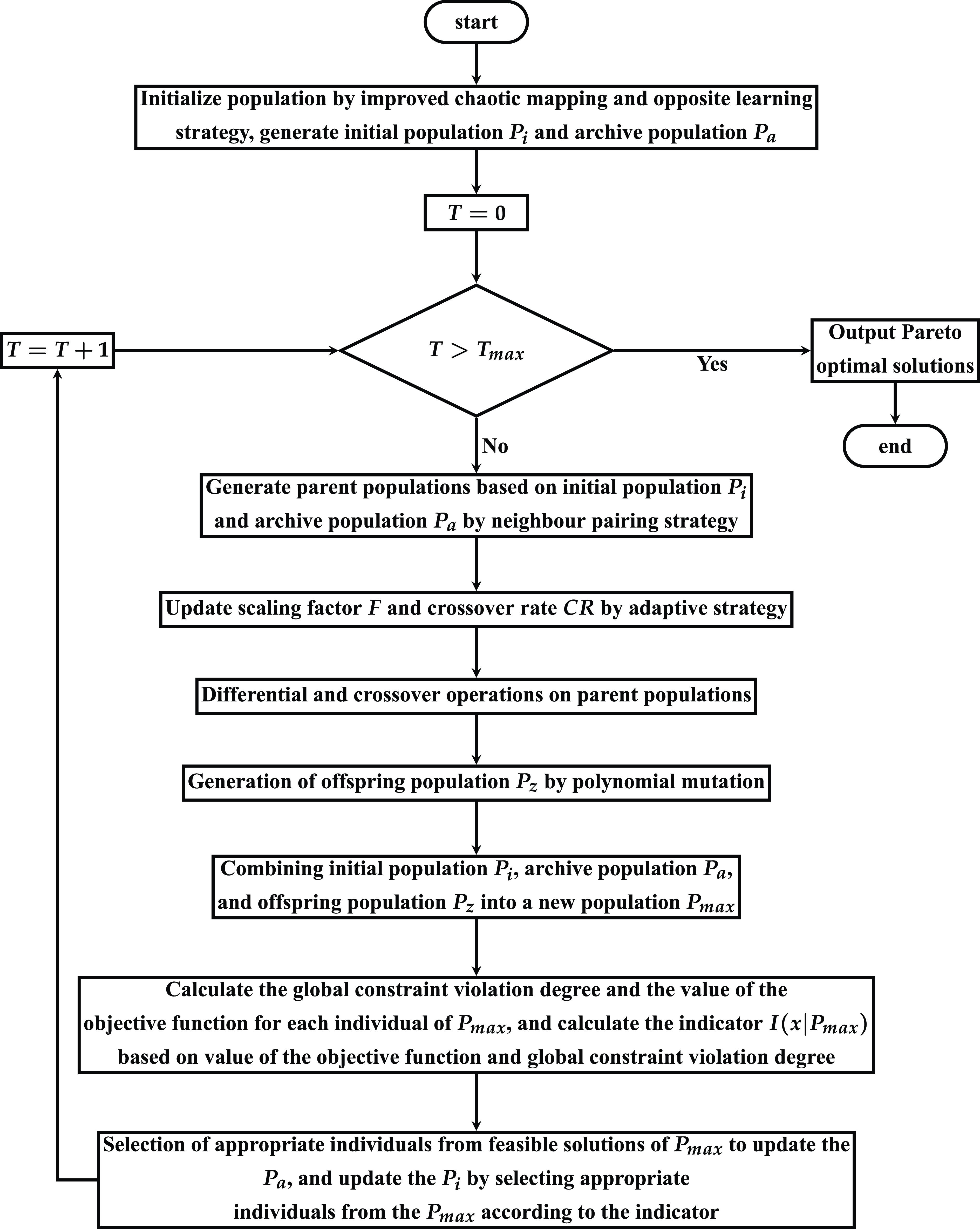
The flow of the proposed optimization algorithm is depicted in Figure 1. Initially, the population $P_{i}$ is generated using an enhanced Tent chaotic mapping with the opposition-based learning strategy. Concurrently, a duplicate population $P_{a}$ is established as an archive population. This archive serves to preserve the optimal feasible individuals produced by the algorithm during each iteration. Subsequently, populations $P_{i}$ and $P_{a}$ are amalgamated into a novel population based on a predetermined ratio. This newly formed population is then partitioned into multiple parent populations utilizing a neighbor pairing strategy. Then, the parameters of the differential evolution operator are refined utilizing the proposed adaptive strategy. Subsequently, the parameters of the differential evolution operator are refined using the proposed adaptive strategy. The parent population, derived from the preceding step, serves as the input to execute the suggested adaptive differential evolution algorithm, resulting in the offspring population $P_{z}$ . Following this, the populations $P_{i}$ , $P_{a}$ , and $P_{z}$ are amalgamated into a new population, denoted as $P_{\max}$ .

Figure 1.

The optimization algorithm flowchart.

$P_{i}$ and $P_{a}$ need be revised following the acquisition of the population $P_{\max}$ . The following is the process of updating the population $P_{i}$ using an indicator-based approach: at first, calculate the indicator value of each individual in $P_{\max}$ according to Eq. (26), and filter the individuals in the promising region from $P_{\max}$ to form a subset $P_{sub}$ according to Eq. (31). Second, the algorithm evaluates if the number of individuals in $P_{sub}$ equals that in $P_{i}$ . If $P_{sub}$ has fewer individuals than $P_{i}$ , those with superior indicators are chosen from the remaining individuals in $P_{max}$ to fill the gap. Conversely, if $P_{sub}$ exceeds the count in $P_{i}$ , it becomes imperative to evenly divide the promising region and allocate the individuals in $P_{sub}$ across each delineated subregion. Subsequently, one must identify the subregion with the highest density of individuals and remove those exhibiting the poorest metrics. The refined $P_{sub}$ , comprising the survivors, is then poised to engage in the subsequent iteration as the updated $P_{i}$ .

The primary procedure for updating the $P_{a}$ is delineated as follows: initially, the degree of constraint violation for each individual is computed in accordance with Eq. (28). Subsequently, feasible individuals are culled from $P_{\max}$ to constitute a novel population, $P_{a}$ . The subsequent step involves assessing whether the quantity of individuals within the newly formed $P_{a}$ aligns with that of the original $P_{a}$ . In instances where the new $P_{a}$ possesses fewer individuals, those exhibiting minimal constraint violation degree are selected from remaining individuals in $P_{\max}$ to augment it. Conversely, if the new $P_{a}$ harbors an excess of individuals, the environmental selection strategy inherent to PREA [Reference Yuan, Liu, Gu, Zhang and He29] is employed to select individuals equivalent to the count in the original $P_{a}$ . Ultimately, the chosen individuals coalesce to form a new $P_{a}$ population, poised to engage in the subsequent iteration of the algorithm.

(31) \begin{equation} P_{sub} = \{x|I(x|P_{\max}) \geq 0, x \in P_{\max}\} \end{equation}

3.3. Selection of optimal trajectories in Cartesian space

In the realm of robot manipulator trajectory planning, it is often observed that a trajectory designed in joint space may not adequately accommodate the motion of the robot manipulator’s end in Cartesian space. Direct trajectory planning within Cartesian space. However, necessitates substantial computational resources to determine the kinematic inverse solution. Moreover, this approach carries the risk of encountering singularities, which could result in uncontrolled joint velocities. Therefore, this research proposes a method that allows for the consideration of trajectories in Cartesian space during joint space trajectory planning. The objective of this method is to identify an optimal trajectory from the Pareto optimal solutions procured by the optimization algorithm. This trajectory should bear the closest resemblance in shape to the desired path within Cartesian space. The selection of an appropriate metric to gauge the similarity of trajectory shapes in Cartesian space is paramount.

The Fréchet distance is frequently employed to quantify the similarity between curves in spatial representations [Reference Gudmundsson, van Renssen, Saeidi and Wong30]. It can be defined as

(32) \begin{equation} \delta _{F}(T, S) = \inf _{\alpha, \beta }\max _{t \in [0,1]}{d(T(\alpha (t)), S(\beta (t)))} \end{equation}

where T and S denote two successive curves in Cartesian space; $\alpha$ and $\beta$ represent two functions that operate over the interval [0,1]; d represents the distance metric function within Cartesian space; and $\delta _{F}(T, S)$ is the Fréchet distance between T and S. When the curve T is close to the curve S, the $\delta _{F}(T, S)$ is smaller; if reversed, the $\delta _{F}(T, S)$ is larger. By choosing the optimal trajectory from the Pareto optimal solutions, which has the smallest Fréchet distance $\delta _{F}(T, S)$ from the desired path in Cartesian space, it is feasible to conduct joint space trajectory planning while simultaneously meeting the end motion requirements of the robot manipulator in Cartesian space.

4.1. Establishment of robot manipulator motion model and initialization of trajectory planning methods

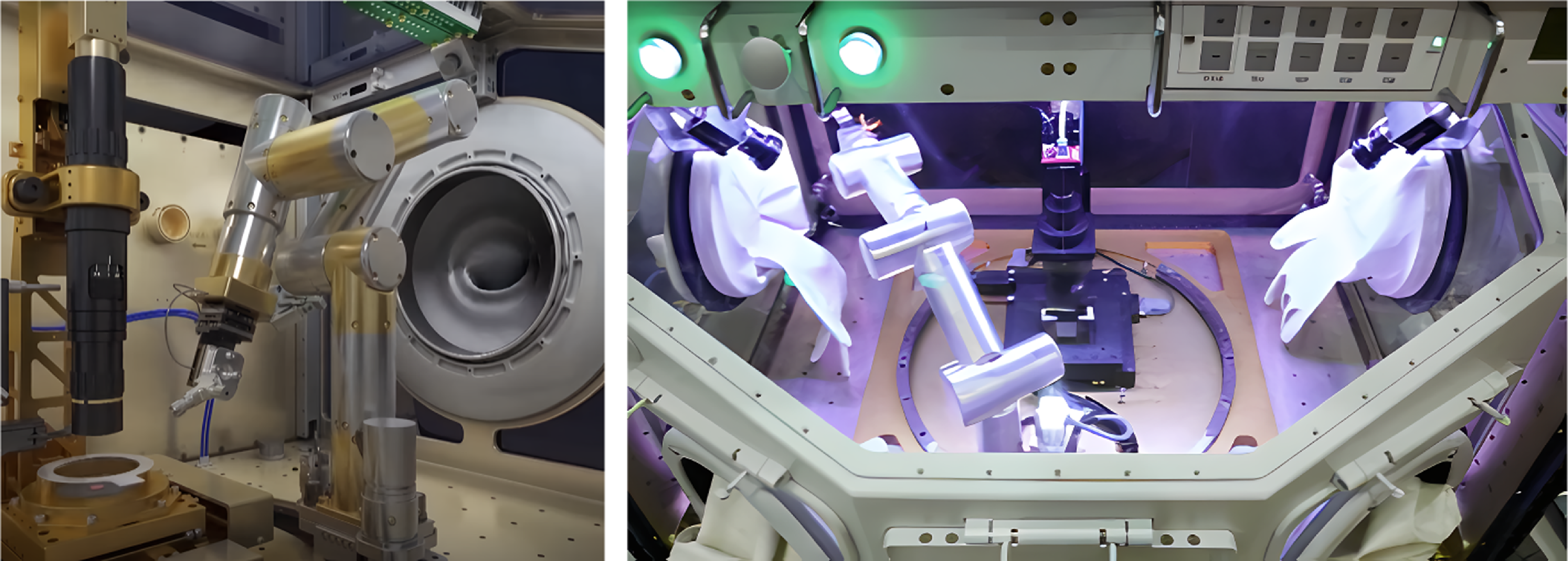
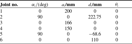
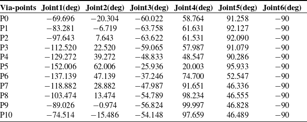
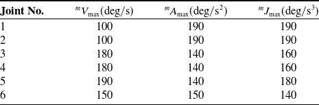
Path data obtained from the robotic arm platform in the experimental cabinet in the Wentian Lab Module were used to validate the effectiveness of the trajectory planning approach. Figure 2 shows a prototype of the robotic arm in the experimental cabinet. The trajectory planning of this robotic arm requires the creation of a corresponding kinematic model. The D-H parametric method is frequently employed to model the kinematics of a robotic arm and to determine both the forward and inverse kinematic solutions. In this study, the planned joint space trajectories need to be obtained by solving the kinematic inverse of the robotic arm model to get the corresponding end trajectories. The standard D-H parameters of the experimental cabinet robot manipulator are listed in Table I. With D-H parameters and inverse kinematics, path points in Cartesian space can be transformed into the via-points in joint space. The via-points in joint space are shown in Table II. The velocity constraints, acceleration constraints, and jerk constraints for each joint are shown in Table III.

Figure 2.

The robotic arm of the experiment cabinet in the space station.

All experiments and simulations are implemented on MATLAB R2023b on a PC running Windows x64, a 13th Gen Intel(R) Core (TM) i5-13600KF @3.50 GHz CPU, and 32 GB of RAM. The codes of the optimization algorithms used are taken from PlatEMO [Reference Tian, Cheng, Zhang and Jin31], a MATLAB platform for multi- or many-objective optimization. At the beginning of the experiment, the population size is set to 200, and the maximum number of function evaluations is set to 100,000. The upper limit of the time interval is 5 s, and the lower limit of the time interval is 0.5 s. The parameter $\alpha$ of Tent chaotic mapping is 0.499. The weight factor $w_{cr}$ is 0.9. The rate of change adjustment parameter q is 0.6.

Table I.

D-H parameters of the robot manipulator.

4.2. Optimization method performance validation

The comparative experiments were designed to validate the efficacy and superiority of the proposed constrained multi-objective optimization method in addressing the trajectory planning problem for the experimental cabinet robot manipulator. Five advanced constrained multi-objective optimization algorithms were selected as benchmarks: Coevolutionary constrained multi-objective optimization (CCMO) [Reference Tian, Zhang, Xiao, Zhang and Jin32], Two-stage evolutionary algorithm with three indicators (TSTI) [Reference Dong, Gong, Ming and Wang33], NSGA-II [Reference Deb, Pratap, Agarwal and Meyarivan34], Evolutionary multitasking-based constrained multiobjective optimization (EMCMO) [Reference Qiao, Yu, Qu, Liang, Song and Yue35], and NSGA-III [Reference Deb and Jain36]. The objective of this experiment was to employ suitable indicators to assess the optimization results of the algorithm. Within the realm of constrained multi-objective optimization, two evaluation indicators are commonly employed: inverted generational distance plus (IGDp) and hypervolume (HV). Both indicators serve to evaluate the performance of the algorithm and the quality of the Pareto optimal solutions derived [Reference Cai, Xiao, Li, Hu, Ishibuchi and Li37, Reference Zitzler, Brockhoff, Thiele, Obayashi, Deb, Poloni, Hiroyasu and Murata38].

Table II.

Via-points in joint space.

Table III.

Velocity, acceleration, and jerk constraints for robot manipulator.

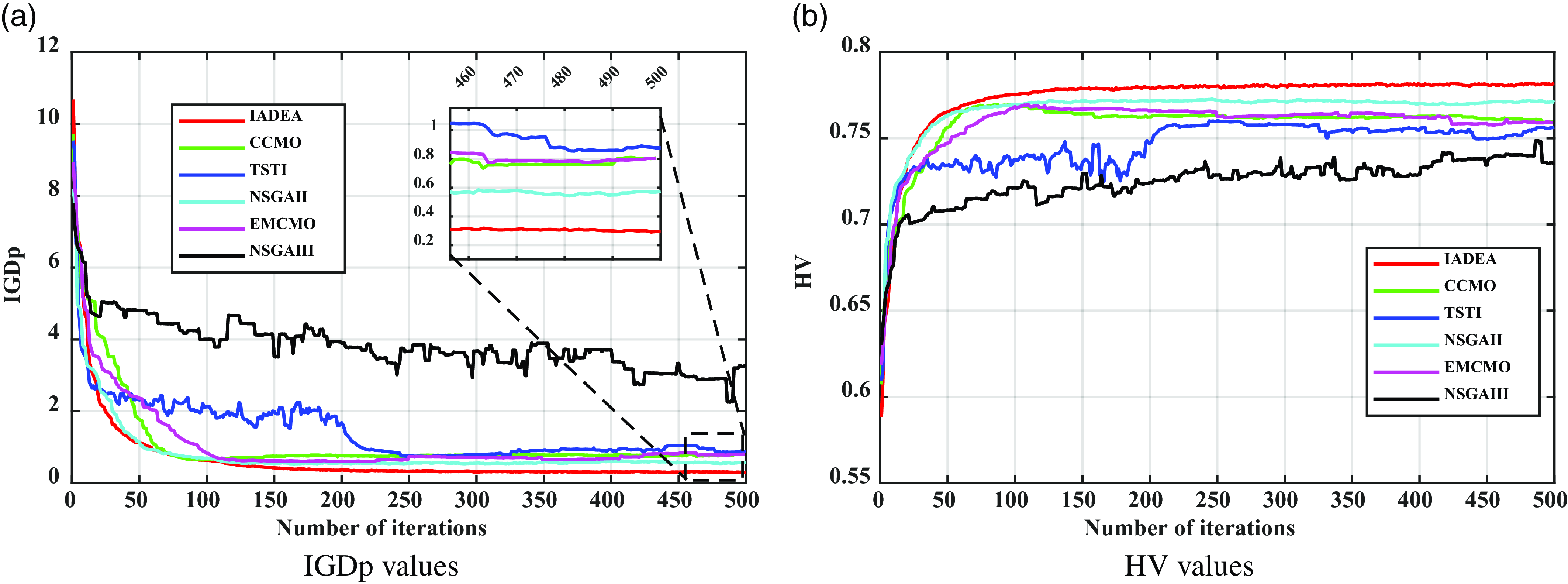
The IGDp is an enhanced version of the IGD, developed to rectify its non-compliance with the Pareto criterion. This indicator gauges the distance between the algorithm’s Pareto optimal solutions in the objective space and the actual constrained Pareto solutions. A smaller IGDp signifies that the solutions derived from the algorithm are closer to the true constrained Pareto optimal solutions, suggesting a superior solution quality. Nonetheless, computing this indicator necessitates knowledge of the genuine solutions, which is typically elusive in real-world engineering problems. Numerous scholars have suggested using approximate constrained Pareto optimal solutions as the benchmark for the IGDp. This study employs a gridding technique introduced in ref. [Reference Cai, Xiao, Li, Hu, Ishibuchi and Li39] to determine the approximate constrained Pareto optimal solutions, subsequently utilizing these solutions to compute the IGDp. The IGDp for various optimization algorithms on robot manipulator trajectory planning is depicted in Figure 3(a).

Figure 3.

Convergence profiles of the six algorithms.

The HV indicator denotes the volume bounded by the Pareto optimal solutions derived from the optimization algorithm and the reference point within the objective space. A larger HV indicator signifies a more widely dispersed Pareto optimal solutions, indicating superior solution quality and enhanced algorithm performance. Figure 3(b) presents the HV for various optimization algorithms addressing robot manipulator trajectory planning.

Table IV.

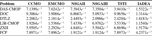
IGDp indicators for each algorithm on other optimization problems.

Table V.

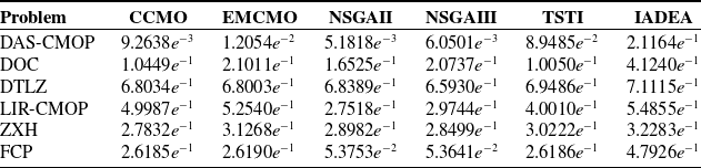
HV indicators for each algorithm on other optimization problems.

To assess the efficacy of the proposed multi-objective optimization algorithm, it was applied to six representative multi-objective optimization problems and its performance was juxtaposed with other algorithms of a similar nature. The selected problems encompassed DAS-CMOP [Reference Fan, Li, Cai, Li, Wei, Zhang, Deb and Goodman40], DOC [Reference Liu, Wang and Tang41], DTLZ [Reference Deb, Thiele, Laumanns, Zitzler, Abraham, Jain and Goldberg42], LIR-CMOP [Reference Fan, Li, Cai, Huang, Fang, You, Mo, Wei and Goodman43], ZXH [Reference Zhou, Xiang and He44], and FCP [Reference Yuan, Liu, Ong and He28]. Tables IV and V present the IGDp and HV metrics for these six problems, incorporating the results from the proposed IADEA algorithm. In the six constrained multi-objective optimization problems examined, the HV indicators of the proposed IADEA consistently surpass those of other algorithms. Conversely, the IGDp indicators for IADEA are consistently lower than those of its counterparts. These findings suggest that the proposed IADEA exhibits superior optimization capabilities relative to alternative algorithms within these specific problem sets.

In Figure 3(a) and (b), both TSTI and NSGAIII exhibit significant instability during the initial iterations when compared to other algorithms. In contrast to NSGAIII, TSTI is capable of converging to a stable region after the iteration. However, NSGAIII has yet to achieve this level of stability. The final convergence results indicate that the IADEA algorithm outperforms all five other algorithms. In terms of convergence speed, the IADEA algorithm is initially slower than NSGAII. This is due to the fact that in the early stages of iteration, the IADEA algorithm must guide the population toward a promising region for exploration. As the number of iterations increases, the algorithm transitions from a global search to a local search, thereby accelerating the speed of convergence. Consequently, the IADEA algorithm demonstrates superior overall convergence speed.

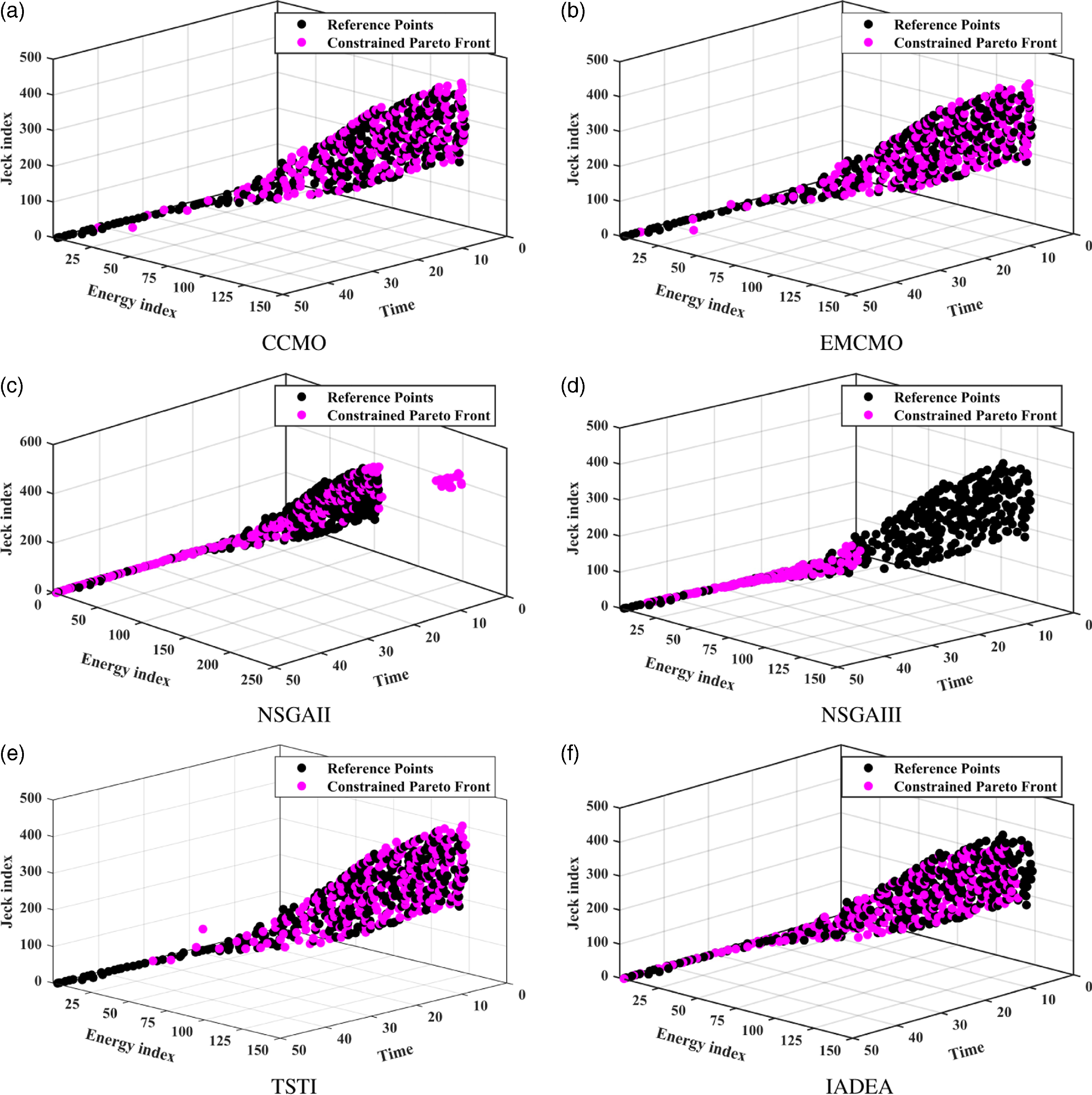
Figure 4 presents the distribution of Pareto optimal solutions within the objective space derived from the six multi-objective optimization algorithms. As illustrated in Figure 4, CCMO, EMCMO, and TSTI, effectively direct the population toward local optimization within regions characterized by minimal time bias and significant energy consumption and jerk. However, these algorithms yield a limited and unevenly distributed number of solutions in regions with large time metrics. Within the region where time metrics fall between 5 and 15 s, NSGAII yields fewer solutions than the proposed IADEA. Furthermore, its distribution lacks uniformity and exhibits a proclivity toward local optima, while NSGAIII exhibits a pronounced local stagnation. In contrast, the proposed IADEA demonstrates superior capability in guiding the population to explore within the target space, thereby yielding Pareto solutions characterized by a more balanced distribution and enhanced diversity.

Figure 4.

Constrained Pareto solutions in objective space of individual optimization algorithms.

4.3. Results of trajectory planning and analysis

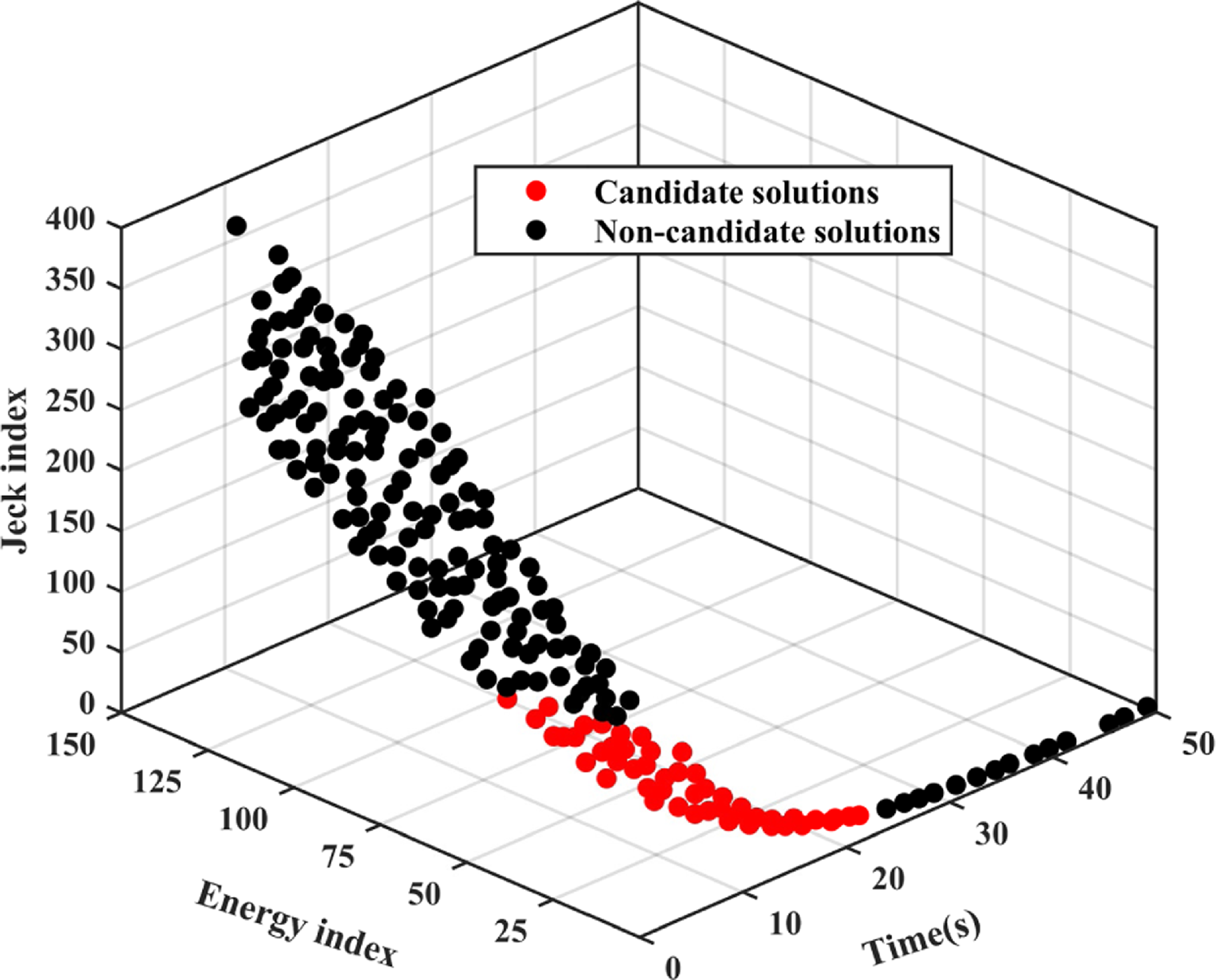
In this section, the complete trajectory planning process is discussed. Initially, the joint space trajectory is established by interpolating the via-points in Table II using the seventh-degree B-spline curve. Subsequently, this trajectory is optimized through the application of the proposed multi-objective optimization algorithm. In this process, the time interval between each pair of path points serves as the decision variable. The optimized results are depicted in Figure 5.

Figure 5.

Solutions with relatively superior overall performance.

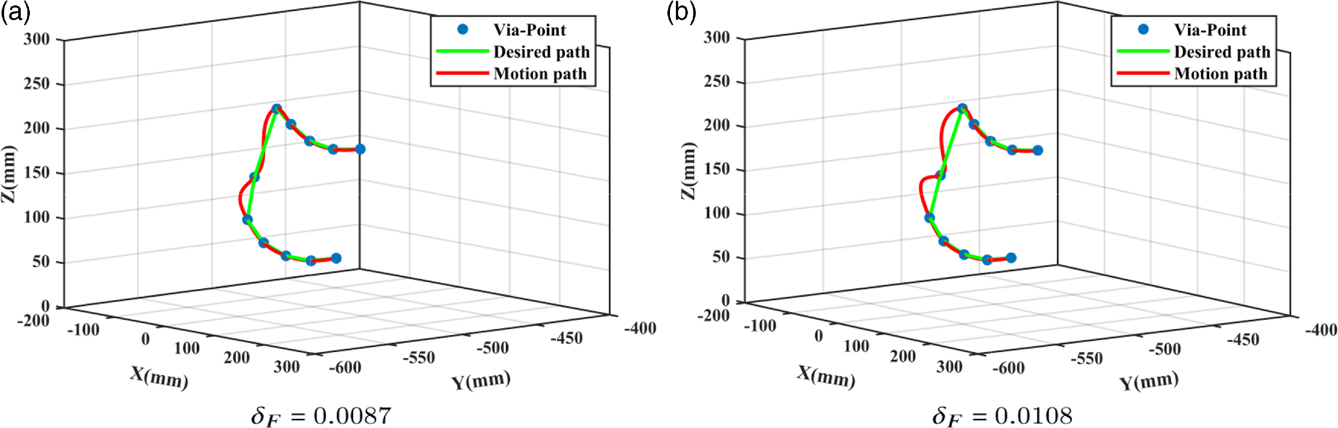
The red section in Figure 5 denotes the candidate region within the Pareto solutions, a collection of solutions exhibiting superior performance. By computing the Fréchet distance for each trajectory associated with a solution in this region and subsequently ranking them, the solution linked to the smallest Fréchet distance can be pinpointed. The minimum Fréchet distance, $\delta _F$ , of the optimal trajectory derived from this solution is 0.0087. The maximum Fréchet distance among the trajectories procured in the candidate region stands at $\delta _F$ = 0.0108. A visualization of these two trajectories in Cartesian space is depicted in Figure 6. In this figure, blue points signify the robot manipulator’s passing points in Cartesian space, green curves illustrate the anticipated movement path of the robot manipulator’s end-effector in Cartesian space, and red curves represent the optimized motion trajectory of the same end-effector in Cartesian space. A comparison between Figure 6(a) and (b) reveals that the optimized trajectory in Figure 6(a) aligns more closely with the expected motion path, whereas the trajectory in Figure 6(b) deviates significantly from it.

Figure 6.

The paths with different Fréchet distances in Cartesian space.

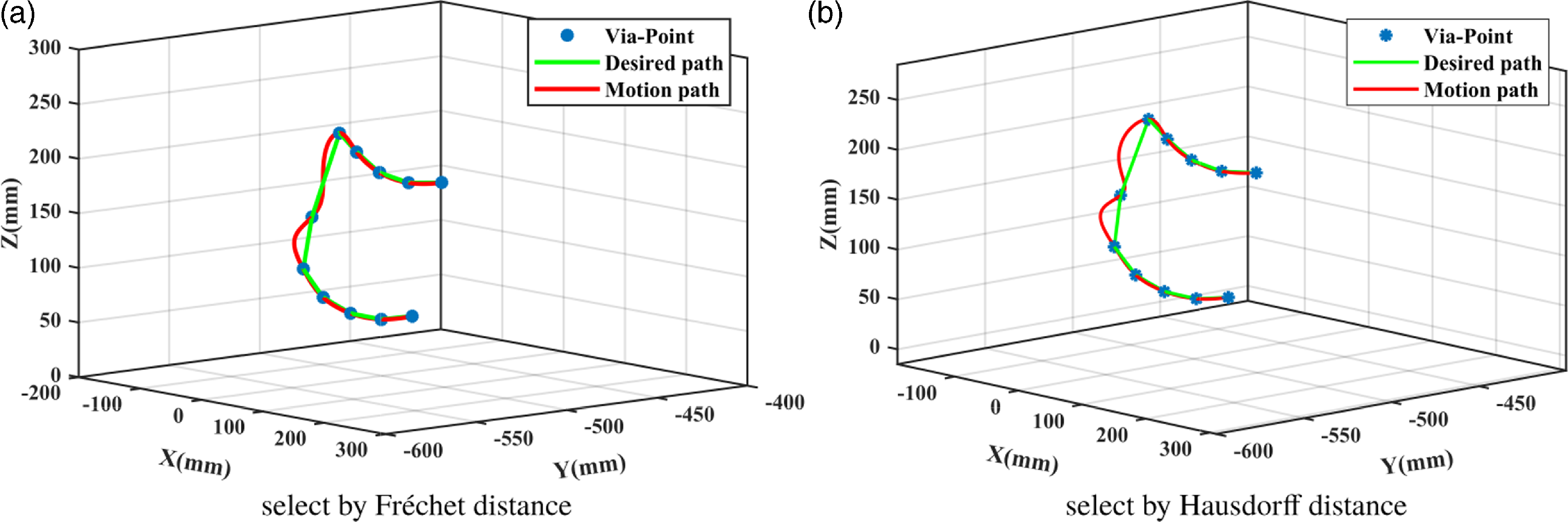
To validate the superiority of the Fréchet distance in measuring path similarity, this study juxtaposes the trajectory derived from the Fréchet distance with that obtained via the Hausdorff distance [Reference Alt and Scharf45], which is usually used to measure the similarity of curves. Figure 7 shows the comparison between the Cartesian space paths selected by two different distances and the desired path. It is evident that the path derived from the Fréchet distance more closely aligns with the desired trajectory than the Hausdorff distance.

Figure 7.

The trajectories selected by different distances in Cartesian space.

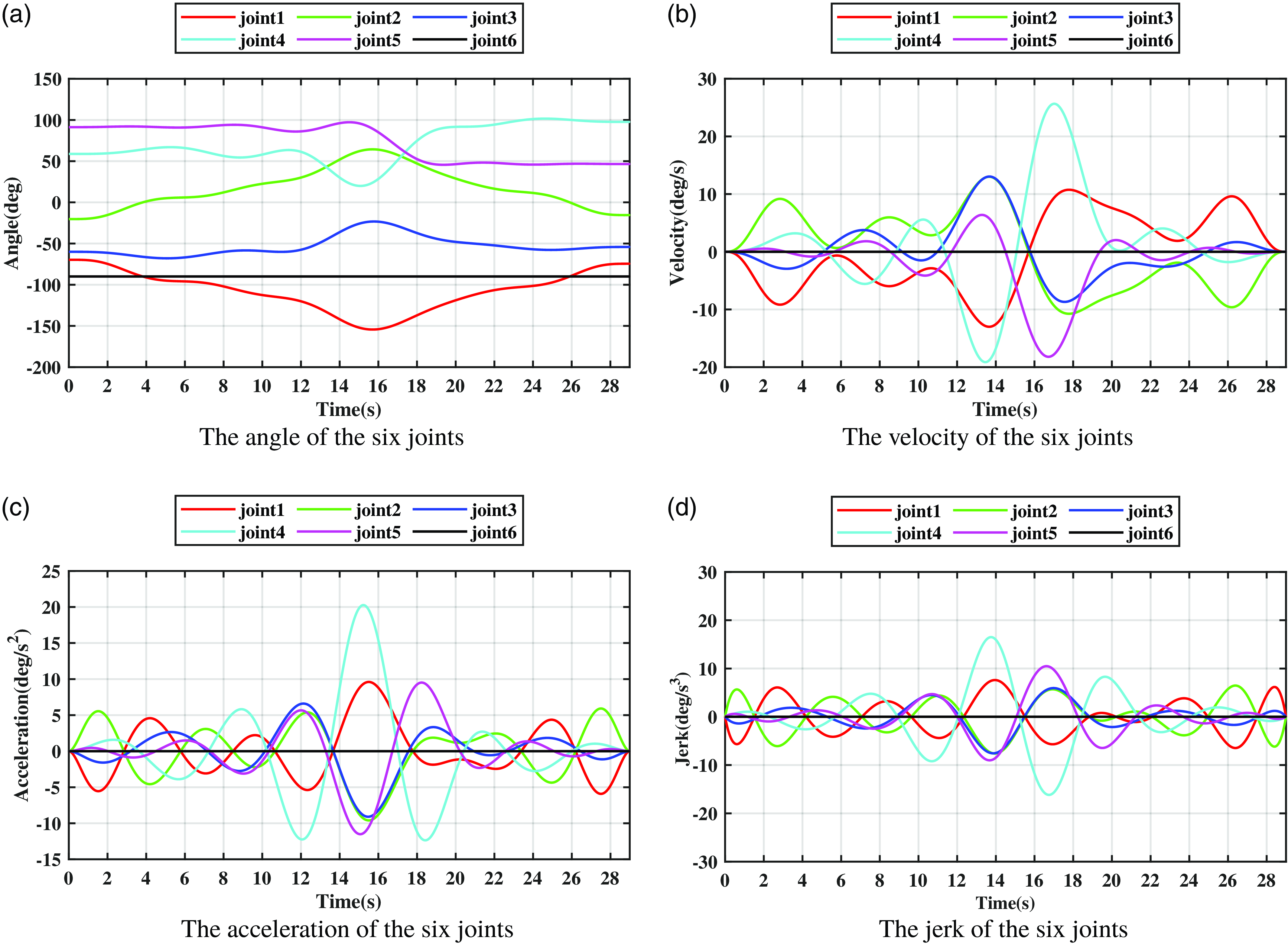
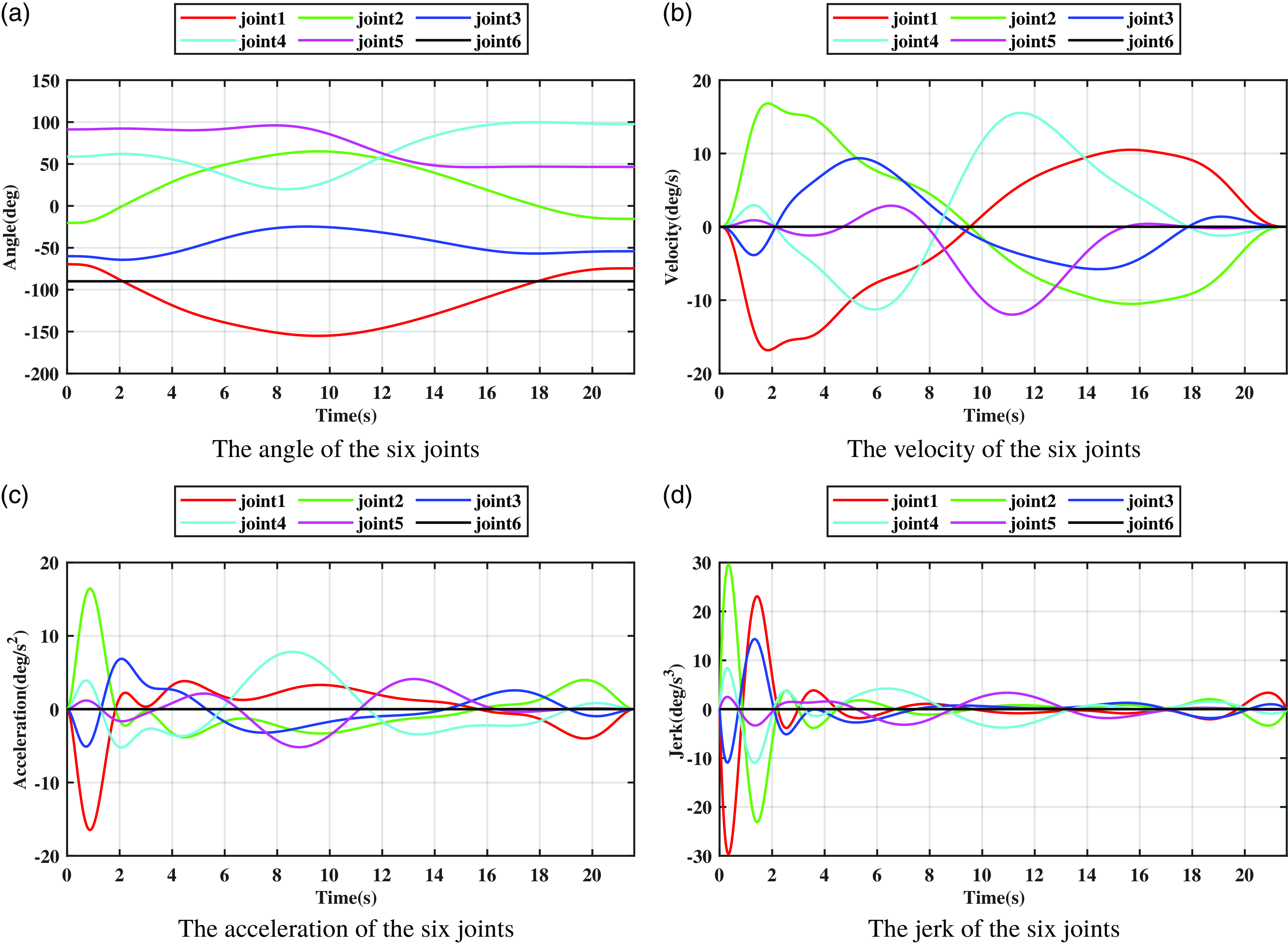
Figures 8 and 9 illustrate the joint space trajectories produced by the B-spline interpolation method alone and those generated by the proposed trajectory planning method, respectively. Upon comparing these two trajectories, it becomes evident that the trajectory produced by the B-spline interpolation method exhibits larger amplitude and higher frequency oscillations in velocity, acceleration, and jerk. This is highly detrimental to the movement of the robotic arm, causing frequent joint jitter during operation. The trajectory generated by the proposed trajectory planning method is smoother and the continuity of the trajectory is better.

Figure 8.

The joint space trajectory obtained using only B-spline interpolation.

Figure 9.

The joint space trajectory derived from the proposed trajectory planning method were utilized.

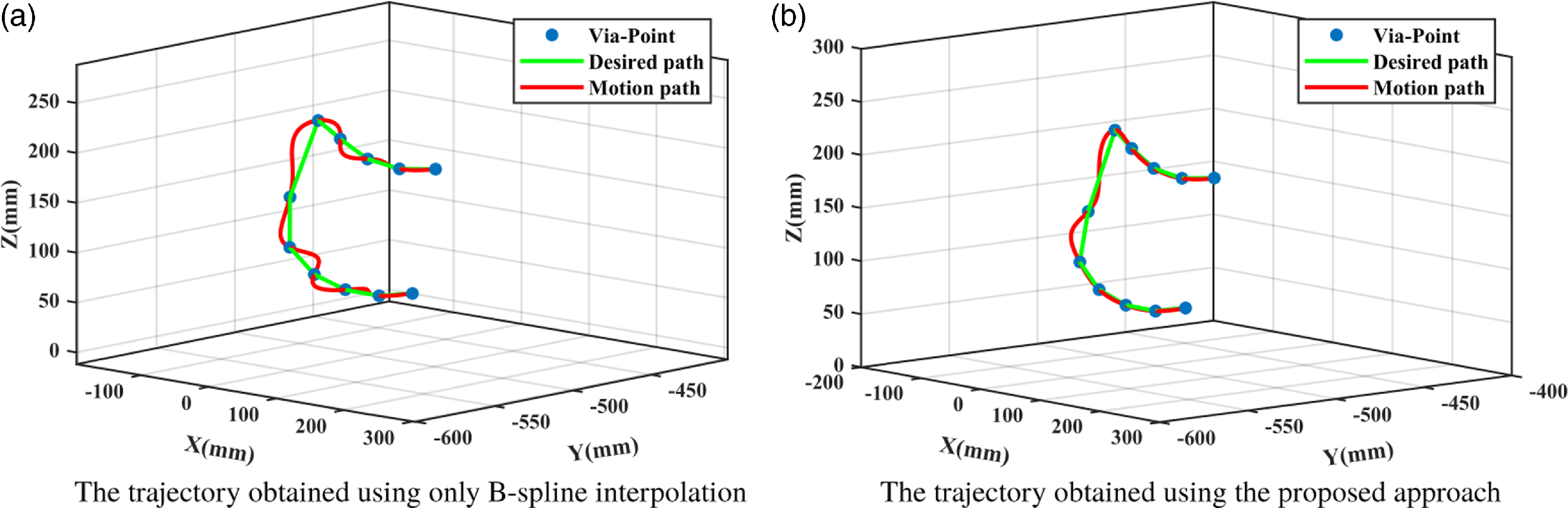
Figure 10 shows the Cartesian space trajectory produced by the B-spline interpolation method alone and those generated by the proposed trajectory planning method, respectively. When only B-spline interpolation is used, the Cartesian space trajectory’s shape is suboptimal. However, following the application of the proposed trajectory planning method, the resulting Cartesian space trajectory more closely aligns with the desired path shape. This enhancement ensures that the robot arm’s endpoint moves along the intended path in Cartesian space.

Figure 10.

Cartesian trajectories generated using different methods.

Table VI presents the performance metrics for unoptimized trajectory and optimized trajectory, respectively. The trajectory of the robotic manipulator, without the application of trajectory planning, yields time, energy consumption, and jerk indicators of 29.0 s, 10.9986, and 12.3797 deg/ ${\rm s}^{3}$ respectively. Conversely, when trajectory planning is employed, these indicators are reduced to 21.5974 s for time, 9.0663 for energy consumption, and a notably lower 4.1616 deg/ ${\rm s}^{3}$ for jerk. Compared to a trajectory that lacks trajectory planning, the trajectory derived from trajectory planning reduces time, energy consumption, and impact by 25.53%, 17.56%, and 66.38%, respectively.

Table VI.

Comparison between unoptimized trajectory and optimized trajectory.

4.4. Evaluation of interpolation performance

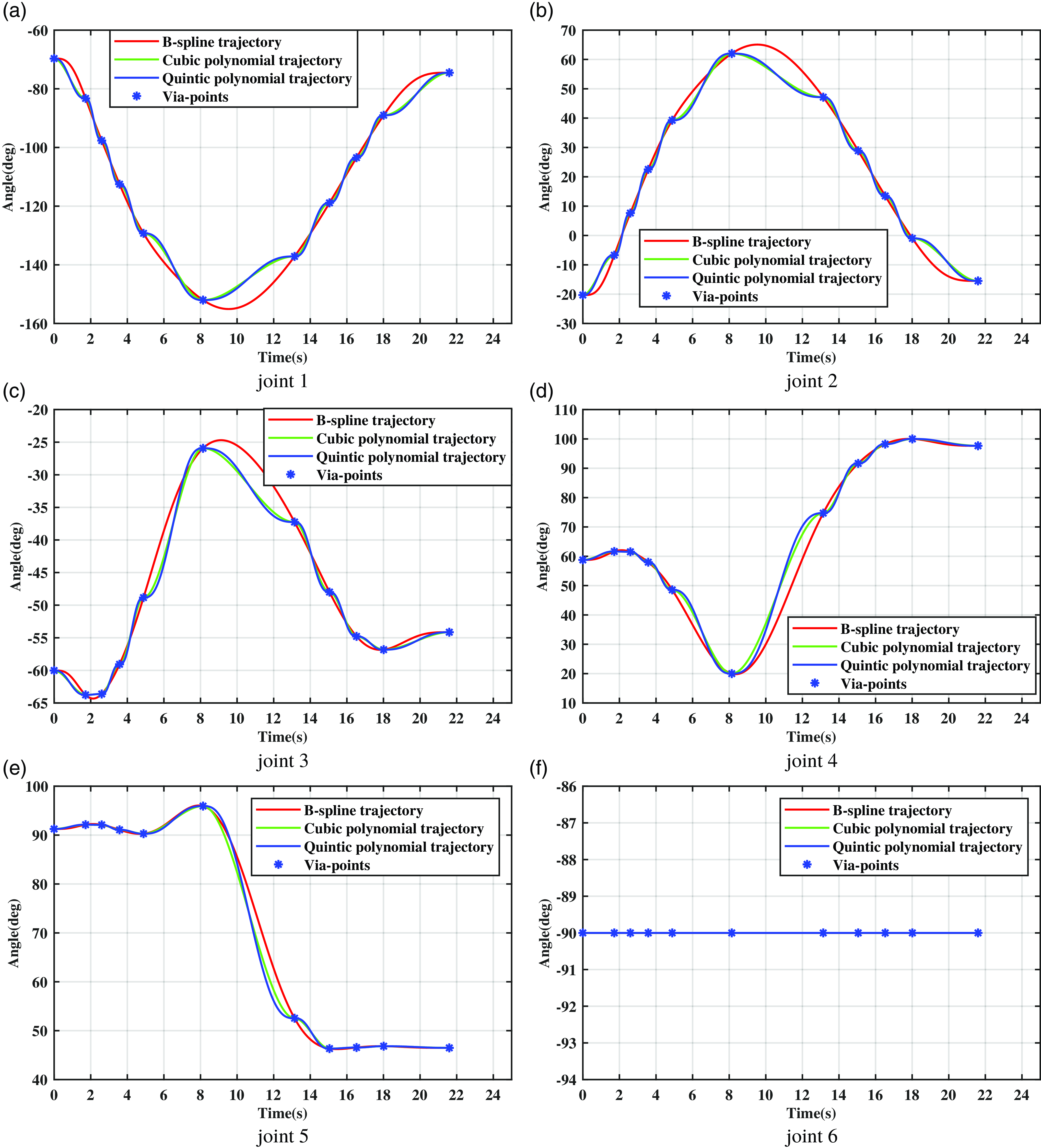
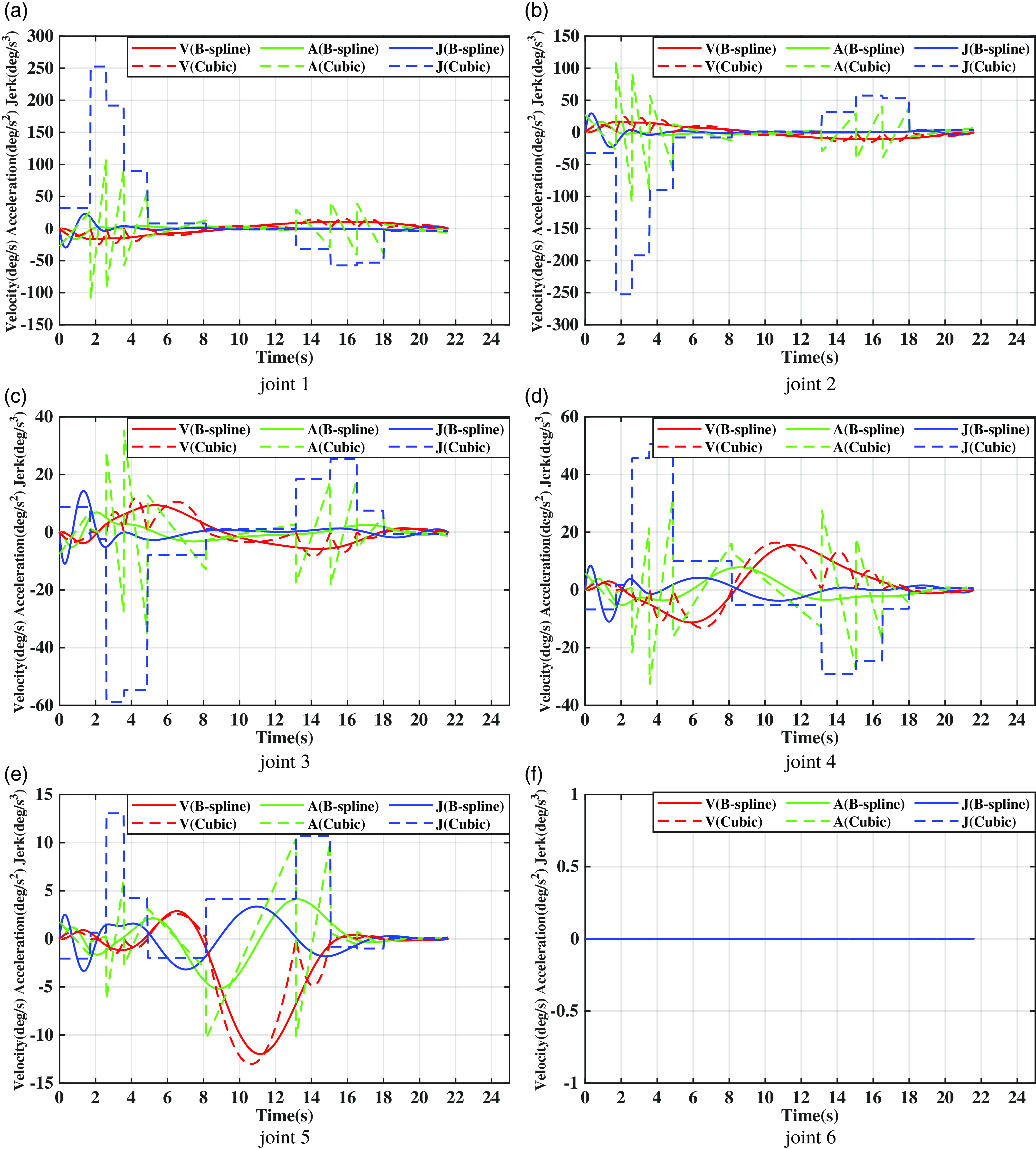
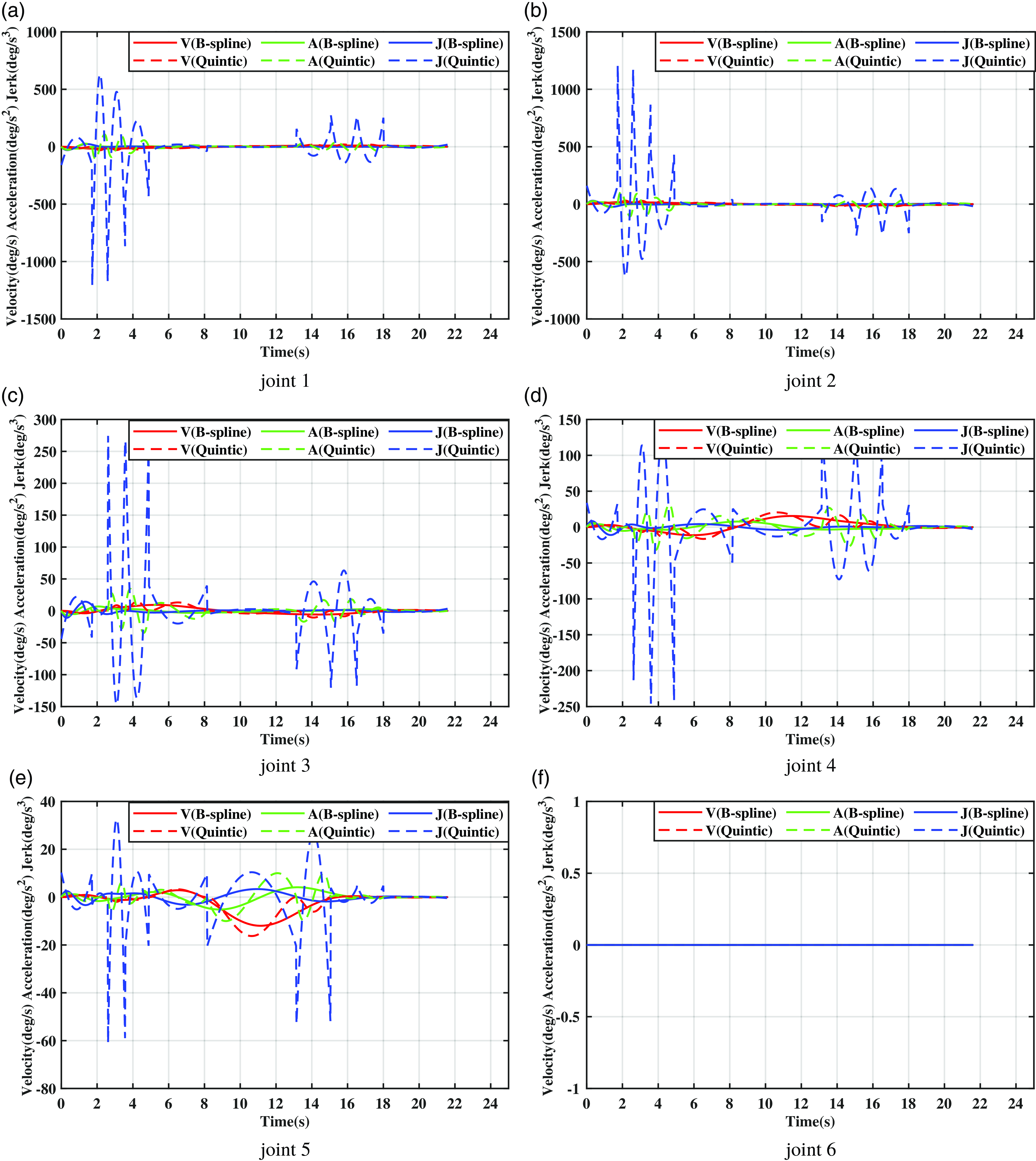
To assess the interpolation efficacy of the curves, we compare B-spline curves with the prevalent cubic polynomial and quintic polynomial curves. The time required to generate these trajectories is determined using our proposed optimization algorithm. Figures 11, 12, and 13 show a comparison of the three curves for joint angle, joint velocity, joint acceleration, and jerk during the working. The three figures illustrate that the trajectories derived from cubic polynomial interpolation can only ensure continuity in joint angle and joint velocity, while their joint acceleration and jerk are discontinuous. Conversely, those obtained from quintic polynomial interpolation can guarantee continuity in joint angle, joint velocity, and joint acceleration, but not in jerk. When compared to these two types of curve interpolation, the trajectories derived from seventh-degree B-spline interpolation can simultaneously satisfy the continuity of joint angle, joint velocity, joint acceleration, and jerk. Furthermore, they allow for the setting of initial velocity, acceleration, and jerk values as per requirements. Additionally, the seventh-degree B-spline curve trajectory exhibits smaller acceleration and jerk peaks compared to the other two types of curves, thereby generating a more stable and smoother trajectory.

Figure 11.

Joint angles generated by different curves.

Figure 12.

Joint velocities, joint accelerations, and jerks generated using cubic polynomials and B-spline interpolation, respectively.

Figure 13.

Joint velocities, joint accelerations, and jerks were generated using quintic polynomials and B-spline interpolation, respectively.