




1 Introduction
The dynamical processes by which a fluid within a spinning container attains the same angular velocity as the vessel is referred to as the ‘spin-up’ (or ‘spin-down’) problem, and was unified in the theoretical treatment of Greenspan & Howard (Reference Greenspan and Howard1963) (hereafter GH). Suppose that the vessel is a right solid of horizontal dimension  $L$ containing an isothermal fluid of viscosity
 $\unicode[STIX]{x1D708}$. At
 $t=0$ the container is rotated about its vertical axis with a constant angular velocity
 $\unicode[STIX]{x1D6FA}$. The fluid takes a finite amount of time to ‘spin up’ to the angular velocity of the solid container. Clearly, were the required transfer of angular momentum controlled solely by viscosity the spin-up time would scale as
 ${\unicode[STIX]{x1D70F}_{s}}^{\unicode[STIX]{x1D708}}\propto L^{2}/\unicode[STIX]{x1D708}$. However, GH showed that
 $\unicode[STIX]{x1D70F}_{s}=\unicode[STIX]{x1D6FA}^{-1}Re^{1/2}$, where the Reynolds number is
 $Re=L^{2}\unicode[STIX]{x1D6FA}/\unicode[STIX]{x1D708}$, and hence
 ${\unicode[STIX]{x1D70F}_{s}}^{\unicode[STIX]{x1D708}}/\unicode[STIX]{x1D70F}_{s}\propto Re^{1/2}$. Therefore, given that
 $Re$ is typically large, the time required for fluid spin up is much smaller than if the process were controlled by viscosity alone.
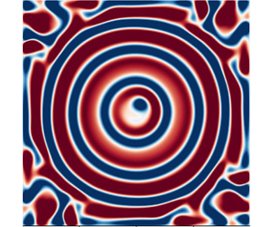
When the surfaces of the container are heated, the interplay between buoyancy and rotational forces complicates the dynamics considerably. For example, when the container is heated from below, the long-term ( $\unicode[STIX]{x1D70F}\gg \unicode[STIX]{x1D70F}_{s}$) state is characterized by columnar vortices aligned in the direction of gravity, along which fluid buoyancy is transported. Here, we study the spin up of a convectively unstable impulsively rotated container of fluid to its final vortical state. In particular, we are interested in a transient ring pattern that occurs during convective spin up. This ringed state consists of alternating axisymmetric rings of up- and downwelling flow, which have been observed experimentally by Boubnov & Golitsyn (Reference Boubnov and Golitsyn1986), Vorobieff & Ecke (Reference Vorobieff and Ecke1998) and Zhong, Patterson & Wettlaufer (Reference Zhong, Patterson and Wettlaufer2010).
The experiments of Boubnov & Golitsyn (Reference Boubnov and Golitsyn1986) were performed in square and circular cross-sectioned containers of water with open upper surfaces cooled by evaporation. They measured the temperature of the free surface and estimated the rate of evaporation, and hence the cooling rate, to be nearly steady. When the upper surface was one of free slip, they observed the transient ringed state for a wide range of rotation and cooling rates (varied by changing the mean temperature of the water). However, for both square and circular cross-sections, when the top surface was covered by a lid, and the bottom surface is heated, they found no ringed state.
In contrast to Boubnov & Golitsyn (Reference Boubnov and Golitsyn1986), Vorobieff & Ecke (Reference Vorobieff and Ecke1998) held the bottom surface at constant temperature and found the ringed state (albeit with fewer rings) in a cylindrical container with a no-slip upper surface. Zhong et al. (Reference Zhong, Patterson and Wettlaufer2010) combined particle image velocimetry with infrared thermometry in a square cross-section container of depth  $H$ with an evaporating free-slip upper surface. They quantified the ringed state as a transient balance between rotational and viscous forces that exists for approximately one Ekman time,
 $\unicode[STIX]{x1D70F}_{E}=\sqrt{H^{2}/\unicode[STIX]{x1D6FA}\unicode[STIX]{x1D708}}$.
Here, we study the formation and breakdown of these transient convective rings using numerical simulations in a variety of geometries. We find that the ringed state is a generic feature of convective spin up under suitable boundary conditions. For other boundary conditions, the rings take on the shape of the container, leading to square ‘sheets’ of convection for square cross-sectioned geometries. We also find that the Prandtl number plays an important role in the formation and stability of the rings. Additionally, we find that the thermal boundary conditions used – Dirichlet as in Vorobieff & Ecke (Reference Vorobieff and Ecke1998) and Neumann as in Boubnov & Golitsyn (Reference Boubnov and Golitsyn1986) and Zhong et al. (Reference Zhong, Patterson and Wettlaufer2010) – influence the rings’ stability and the dynamics of their breakdown. Our results reconcile the seemingly contradictory observations of Boubnov & Golitsyn (Reference Boubnov and Golitsyn1986) and Vorobieff & Ecke (Reference Vorobieff and Ecke1998).
In § 2, we describe the set-up of the numerical simulations and the key differences from the experiments. We then discuss the numerical methods used and the resolution requirements for the simulations. The formation, longevity and breakdown of the ringed state into the final vortical state are summarized in § 3, wherein we also examine some special cases of ring formation in non-standard geometries, and connect these to what is observed experimentally. Conclusions are drawn in § 4.
2 Problem set-up and numerical method
The geometry of the problem. The container  $[-L/2,L/2]\times [-L/2,L/2]\times [0,H]$ is spun about the vertical
 $z$-axis with an angular velocity
 $\unicode[STIX]{x1D6FA}$ starting at
 $t=0$.

A schematic of the system under study is shown in figure 1. We consider a container of width  $L$ and height
 $H$ filled with a Boussinesq fluid of density
 $\unicode[STIX]{x1D70C}$, coefficient of thermal expansion
 $\unicode[STIX]{x1D6FC}$, viscosity
 $\unicode[STIX]{x1D708}$ and thermal diffusivity
 $\unicode[STIX]{x1D705}$, at an initial temperature
 $T_{0}$ that is rotated about the vertical axis starting at
 $t=0$. In a frame of reference rotating with the container the Coriolis effect is present. The lateral surfaces are thermally insulating and the top and bottom surfaces have either thermal Dirichlet conditions or one of these horizontal surfaces has a Neumann boundary condition. Other parameters in the problem include the acceleration due to gravity
 $-g\boldsymbol{e}_{z}$ (gravity and the axis of rotation are both along the
 $z$-axis), and the aspect ratio
 $A=L/H$ (
 $=2$ unless otherwise stated). The dimensional equations are
 $$\begin{eqnarray}\displaystyle & \displaystyle \frac{\text{D}\boldsymbol{u}}{\text{D}t}=-\frac{\unicode[STIX]{x1D735}p}{\unicode[STIX]{x1D70C}}+\unicode[STIX]{x1D708}\unicode[STIX]{x1D6FB}^{2}\boldsymbol{u}-2\unicode[STIX]{x1D6FA}\boldsymbol{e}_{z}\times \boldsymbol{u}+g\unicode[STIX]{x1D6FC}(T-T_{0})\boldsymbol{e}_{z}-\unicode[STIX]{x1D6FC}(T-T_{0})\unicode[STIX]{x1D6FA}^{2}\boldsymbol{r}, & \displaystyle\end{eqnarray}$$
 $$\begin{eqnarray}\displaystyle & \displaystyle \frac{\text{D}T}{\text{D}t}=\unicode[STIX]{x1D705}\unicode[STIX]{x1D6FB}^{2}T & \displaystyle\end{eqnarray}$$
and
 $$\begin{eqnarray}\displaystyle \unicode[STIX]{x1D735}\boldsymbol{\cdot }\boldsymbol{u}=0. & & \displaystyle\end{eqnarray}$$
In the rotating frame the initial velocity of the fluid is
 $$\begin{eqnarray}\boldsymbol{u}|_{t=0}=-\unicode[STIX]{x1D734}\times \boldsymbol{r},\end{eqnarray}$$
and the initial temperature is  $\unicode[STIX]{x1D703}=0$ in the entire container. This is different from the fully developed convective state that is used as the initial condition in the laboratory experiments of Boubnov & Golitsyn (Reference Boubnov and Golitsyn1986) and Zhong et al. (Reference Zhong, Patterson and Wettlaufer2010) prior to spin up.
2.1 Boundary conditions
The boundary conditions (BCs) for velocity and temperature determine the nature of the buoyancy forcing and the details of the spin-up process. In the cuboidal geometry, the six bounding surfaces (the top and bottom surfaces, and the four lateral boundaries) are impenetrable and thus have zero normal velocity. Each boundary can have no-slip or free-slip velocity BCs and Dirichlet ( $T=\text{const}.$) or Neumann (
 $\unicode[STIX]{x2202}T/\unicode[STIX]{x2202}n=\text{const}.$) thermal BCs.
We consider here only cases where the lateral surfaces are insulating (i.e. have zero heat flux) and have identical velocity BCs (free slip or no slip), and the thermal BCs on the top and bottom surfaces are of the same type (either both Dirichlet or both Neumann). Thus there are eight combinations of BCs. Of these, the majority of our results are from the combinations listed (in their non-dimensionalized form) in table 1 in § 2.1 below. Other combinations are mentioned where relevant.
For simplicity we call all boundaries ‘surfaces’, so that, for instance, a ‘free-slip surface’ is a boundary where the normal velocity and the tangential stress are both zero.
Combinations of the BCs used for the results reported. Some other possible combinations are discussed as special cases in § 3.5. BCs of Type I are as used by Boubnov & Golitsyn (Reference Boubnov and Golitsyn1986) (BG) and Zhong et al. (Reference Zhong, Patterson and Wettlaufer2010) (ZPW). Type II is the Vorobieff & Ecke (Reference Vorobieff and Ecke1998) (VE) set-up with a cylindrical container. Comparing results from Type I and Type III (§§ 3.1 and 3.4) elucidates the role of the thermal BCs in the dynamics. BCs of Types IV and V produce no rings, instead producing square sheets of convection.

2.2 Non-dimensionalization
We scale time in the problem using the rotation rate,  $\unicode[STIX]{x1D6FA}^{-1}$, and the length using the width of the container
 $L$ (see figure 1). The choice of
 $L$ instead of
 $H$ for the length scale ensures that the magnitude of the initial velocity is less than unity, thereby facilitating numerical stability. These together define the velocity scale
 $U=L\unicode[STIX]{x1D6FA}$. Assuming a temperature scale
 $\unicode[STIX]{x0394}T$ (to be defined in the case of constant heat flux), the governing equations (2.1)–(2.3) become
 $$\begin{eqnarray}\displaystyle & \displaystyle \frac{\text{D}\boldsymbol{u}}{\text{D}t}=-\unicode[STIX]{x1D735}p+\frac{1}{Re}\unicode[STIX]{x1D6FB}^{2}\boldsymbol{u}-2\boldsymbol{e}_{z}\times \boldsymbol{u}+\frac{1}{Fr^{2}}\,\unicode[STIX]{x1D703}\boldsymbol{e}_{z}, & \displaystyle\end{eqnarray}$$
 $$\begin{eqnarray}\displaystyle & \displaystyle \frac{\text{D}\unicode[STIX]{x1D703}}{\text{D}t}=\frac{1}{Re\,Pr}\unicode[STIX]{x1D6FB}^{2}\unicode[STIX]{x1D703} & \displaystyle\end{eqnarray}$$
and
 $$\begin{eqnarray}\displaystyle \unicode[STIX]{x1D735}\boldsymbol{\cdot }\boldsymbol{u}=0, & & \displaystyle\end{eqnarray}$$
where  $Pr=\unicode[STIX]{x1D708}/\unicode[STIX]{x1D705}$ is the Prandtl number,
 $Re=\unicode[STIX]{x1D6FA}L^{2}/\unicode[STIX]{x1D708}$ is the Reynolds number and
 $Fr^{-2}=g\unicode[STIX]{x1D6FC}\unicode[STIX]{x0394}T/\unicode[STIX]{x1D6FA}^{2}L$ is the Froude number, which is a measure of the strength of the buoyancy relative to other forces, and the centrifugal buoyancy term in (2.1) is neglected. The initial velocity is
 $\boldsymbol{u}(t=0)=-\boldsymbol{e}_{z}\times \boldsymbol{r}$ and the initial temperature is
 $\unicode[STIX]{x1D703}(t=0)=0$ everywhere in the container. The BCs are defined in § 2.1.
A constant heat flux  $\dot{q}$ implies a constant buoyancy flux
 $\tilde{B}$, given in terms of
 $\dot{q}$ as
 $$\begin{eqnarray}\tilde{B}=\frac{g\unicode[STIX]{x1D6FC}\dot{q}}{\unicode[STIX]{x1D70C}C_{p}},\end{eqnarray}$$
where  $C_{p}$ is the heat capacity per unit mass of the fluid at constant pressure. The flux Rossby number, which is a measure of the buoyancy flux, is
 $$\begin{eqnarray}Ro_{f}=\sqrt{\frac{\tilde{B}}{\unicode[STIX]{x1D6FA}^{3}L^{2}}},\end{eqnarray}$$
the flux Rayleigh number  $Ra_{f}$ is
 $$\begin{eqnarray}Ra_{f}=\frac{\tilde{B}H^{4}}{\unicode[STIX]{x1D708}\unicode[STIX]{x1D705}^{2}}=\frac{{Ro_{f}}^{2}Re^{3}Pr^{2}}{A^{4}},\end{eqnarray}$$
and the Nusselt number is
 $$\begin{eqnarray}Nu=\left\langle \frac{\unicode[STIX]{x1D703}^{\prime }H}{\bar{\unicode[STIX]{x1D703}}_{z=0}-\bar{\unicode[STIX]{x1D703}}_{z=H}}\right\rangle ,\end{eqnarray}$$
where  $\unicode[STIX]{x1D703}^{\prime }$ is the constant temperature gradient imposed at
 $z=H$, the overbar
 $\bar{\cdot }$ denotes the spatial average across a given plane, and
 $\langle \cdot \rangle$ denotes the time average. For all the results reported here, the time average was taken over
 $300<t<600$. The standard Rayleigh number follows from the above definitions and is
 $$\begin{eqnarray}Ra=\frac{Ra_{f}}{Nu}.\end{eqnarray}$$
The temperature scale  $\unicode[STIX]{x0394}T$ is defined as
 $$\begin{eqnarray}\unicode[STIX]{x0394}T=\frac{\dot{q}L}{\unicode[STIX]{x1D70C}C_{p}\unicode[STIX]{x1D705}\unicode[STIX]{x1D703}^{\prime }},\end{eqnarray}$$
and hence the Froude number can also be written as
 $$\begin{eqnarray}Fr^{-2}=\frac{{Ro_{f}}^{2}RePr}{\unicode[STIX]{x1D703}^{\prime }}.\end{eqnarray}$$
For very large Taylor numbers,  $Ta=4Re^{2}/A^{4}$, the container of fluid rotates like a solid body, and for small Taylor numbers, the dynamics resembles non-rotating Rayleigh–Bénard convection (Boubnov & Golitsyn Reference Boubnov and Golitsyn1986). The boundary between these is defined by the critical Rayleigh number
 $$\begin{eqnarray}Ra_{c}\propto Ta^{2/3}\propto Re^{4/3},\end{eqnarray}$$
where the constant of proportionality depends on whether the top and bottom surfaces obey free-slip or no-slip BCs (Boubnov & Golitsyn Reference Boubnov and Golitsyn1986).
2.3 Numerical method
The numerical simulations are performed with the finite volume code Megha-5, which uses uniform grids and second-order central differences in space and second-order Adams–Bashforth time stepping. The momentum equation is solved using the projection operator (Chorin Reference Chorin1968) and the resulting Poisson equation for the pressure is solved using cosine transforms with the PFFT Library of Pippig (Reference Pippig2013). The scalar equation is solved using a local upwind scheme (Herrmann, Blanquart & Raman Reference Herrmann, Blanquart and Raman2006) that avoids Gibbs oscillations while retaining overall second-order accuracy. Alternatively, the second-order scheme of Kurganov & Tadmor (Reference Kurganov and Tadmor2000) can also be used. Megha-5 is based on an extensively validated earlier version (Prasanth Reference Prasanth2014) and has been used in studies of jets and plumes (Diwan et al. Reference Diwan, Prasanth, Sreenivas, Deshpande and Narasimha2014), and cumulus (Ravichandran & Narasimha Reference Ravichandran and Narasimha2020) and mammatus clouds (Ravichandran, Meiburg & Govindarajan Reference Ravichandran, Meiburg and Govindarajan2020).
The thickness of the thermal boundary layer adjacent to a surface is defined as the distance at which the mean temperature of the volume would be reached starting at the surface temperature with the slope from the first two gridpoints from the surface, following the convention of Belmonte, Tilgner & Libchaber (Reference Belmonte, Tilgner and Libchaber1994) and Verzicco & Sreenivasan (Reference Verzicco and Sreenivasan2008). We ensure that the thermal boundary layers at the top surface are resolved with at least  $6$ gridpoints for Reynolds numbers
 $Re\leqslant 7.5\times 10^{3}$ (grid size of
 $256^{2}\times 128$, with a time step of
 $2.5\times 10^{-3}$), and up to
 $12$ gridpoints (grid size of
 $512^{2}\times 256$, with a time step of
 $1.25\times 10^{-3}$) for
 $Re\geqslant 10^{4}$, as required in turbulent Rayleigh–Bénard convection (see Scheel, Emran & Schumacher Reference Scheel, Emran and Schumacher2013, and references therein). The results were found to be grid independent and we report those from the lower resolution grid here. We have also verified that the choice of local-upwinding or Kurganov–Tadmor discretization does not affect the results (the former is used here).
Simulations in the cylindrical geometry and the other geometries mentioned in § 3.5 are performed using the volume penalization method (Kevlahan & Ghidaglia Reference Kevlahan and Ghidaglia2001; Schneider & Farge Reference Schneider and Farge2005), with insulating BCs for the simulations in the cylindrical geometry applied following Kadoch et al. (Reference Kadoch, Kolomenskiy, Angot and Schneider2012). We have verified that our results are independent of the penalization parameters used.
3 Results and discussion
Schematic vertical sections through the plane of symmetry of the flow during convective spin up with (a) free-slip top boundary, and all other surfaces no slip; and (b) all surfaces no slip. The arrows show flow directions (magnitudes not to scale). The central dashed line is the axis of rotation (and the direction of gravity). The four labels correspond to (i) flow towards the no-slip surface; (ii) centrifugally outwards flow at a no-slip surface; (iii) flow rising vertically along the lateral boundaries; and (iv) return flow towards the axis of rotation. This pattern and its mirror image are seen in (b).

We begin by summarizing the spin-up process in the absence of buoyancy forcing, following GH. Consider the case where the top surface is one of free slip and the bottom surface and the four lateral boundaries are no-slip surfaces, as shown schematically in figure 2(a). The flow at the bottom surface is that due to a plate impulsively rotated about an axis perpendicular to its plane (see e.g. chap. 5.2.4, p. 119 of Schlichting & Gersten Reference Schlichting and Gersten2016). Fluid is centrifuged outwards from the axis of rotation along the surface. Continuity drives fluid downward towards the bottom surface. As the centrifuged fluid reaches the periphery of the container, it ascends up the lateral surfaces, driven by a vorticity gradient that exists as a result of the boundary layers on the lateral surfaces. Once this fluid reaches the upper free surface, it is driven towards the axis, eventually becoming part of the downward flow. In this manner, fluid is driven from larger to smaller radii. Conservation of angular momentum (excepting for small viscous losses) ensures that the fluid near the axis is replaced with fluid that is rotating more rapidly. GH show that this process takes a time  $O(\unicode[STIX]{x1D6FA}^{-1}Re^{1/2})=O\sqrt{(L^{2}/\unicode[STIX]{x1D708}\unicode[STIX]{x1D6FA})}$.
3.1 Type I BCs
We first discuss results from simulations with Type I BCs (see table 1); the sides and the bottom are all no-slip, thermally insulating surfaces and the upper free-slip surface is driven with a constant heat flux. The dynamical time scale for the circulation shown schematically in figure 2(a) is fast relative to the build up of negatively buoyant fluid at the upper surface. As cold plumes emerge, they are sequentially forced towards the axis of rotation as buoyancy and rotational forces balance, the oldest and more central of which are deeper. A given plume evolves into an axisymmetric ring as this quasi-steady balance is attained, thereby leading to a sequence of upwelling and downwelling ring pairs. Up to three pairs are seen for such  $Re\leqslant 10^{4}$. The rings eventually reach the bottom of the box, where they interact with the boundary layer and are influenced by the shape of the container if a sufficiently long time passes. As the system approaches solid-body rotation, the system must become unstable and break up into cyclonic vortices, in which fluid descends surrounded by regions of slower upwelling flow. While this generic process remains similar across a wide parameter range, the ring and vortex numbers are a function of the Reynolds, flux Rossby and Prandtl numbers. A sequence of images showing this evolution is presented in figure 3, and Hovmöller plots showing the evolution of the azimuthally averaged vertical velocity and temperature are shown in figure 4.
Ring formation in a representative case for Type I BCs. Shown are horizontal cross-sections of the vertical velocity field at a plane  $z\approx 0.47$ which is near the cooled upper surface. The parameters of the problem are
 $Re=7500$,
 $Ro_{f}=0.00442$,
 $Pr=5$. (See figure 4 for a Hovmöller plot showing the time evolution and figure 15 for a sequence of vertical cross-sections.) The evolution for these fields is available as a movie in the supplementary material at https://doi.org/10.1017/jfm.2020.387.

Hovmöller plots for (a) the temperature difference  $\unicode[STIX]{x1D703}-\bar{\unicode[STIX]{x1D703}}$, and (b) the azimuthally averaged vertical velocity
 $w$, where
 $\bar{\unicode[STIX]{x1D703}}$ is the average temperature in the plane
 $z=0.46$ where the plots are made, showing the evolution of the rings. The rings can be seen to form around
 $t=40$, move radially inwards and break down around
 $t=150$ coinciding with the completion of spin up.
 $Re=7500,Ro_{f}=0.00442,Pr=5$, as in figure 3.

To exhibit the heat transport by the rings, we plot the cross-sectional area-averaged dimensionless buoyancy flux, defined as
 $$\begin{eqnarray}\langle B\rangle (z,t)=\frac{1}{Fr^{2}}\int _{-1/2}^{1/2}\int _{-1/2}^{1/2}\,\text{d}x\,\text{d}y(w\unicode[STIX]{x1D703}),\end{eqnarray}$$
for a horizontal section at  $z=0.455$. The first two peaks of buoyancy flux seen in figure 5 correspond to the formation of the first ring and the maximally ringed state respectively.
The buoyancy flux at  $z=0.455$ as a function of time, for
 $Re=7500$ and
 $Pr=5$. The peaks in buoyancy flux, labelled (i) and (ii) in the figure, correspond to the time when the first ring forms and (less precisely to) the time at which the ringed state is maximal respectively. The two dotted vertical lines are at
 $t=130$, approximately when spin up is complete and the rings start to break down; and
 $t=300$, when we begin calculations of time averages. Increasing the Rossby number increases the buoyancy flux imposed at the upper surface. The stages of ring formation (maximal state and breakdown) occur earlier when the flux Rossby number is larger.

In the limit of very small  $Ro_{f}$ (2.9), convection is strongly suppressed. For large
 $Ro_{f}$, the heat flux dominates the effects of rotation. The dynamics of ring formation is most prominent at intermediate values of
 $Ro_{f}$, as found by Boubnov & Golitsyn (Reference Boubnov and Golitsyn1986) and Zhong et al. (Reference Zhong, Patterson and Wettlaufer2010). As
 $Ro_{f}$ increases, the time for the first ring to form decreases and its radius increases.
The Prandtl number strongly influences the dynamics – particularly the stability of the ringed state. For a given  $Re$, as thermal dissipation decreases and
 $Pr$ increases, the rings become thinner. Thus, while the thermal effect increases the ring longevity with
 $Pr$, the associated thinning of the rings enhances the across-ring shear, driving the shear instability (note that the flow moves in opposite directions on either side of a ring) and thereby reducing the ring longevity. Thus, the stability of the rings peaks at an intermediate Prandtl number
 $Pr^{\ast }$. The parameter
 $\unicode[STIX]{x1D6F7}$ measures deviations from axisymmetry of a flow variable
 $\unicode[STIX]{x1D719}$ as
 $$\begin{eqnarray}\displaystyle \unicode[STIX]{x1D6F7}=\int _{0}^{r_{max}}\text{d}r[\unicode[STIX]{x1D719}(x,y,z_{0},t)-\unicode[STIX]{x1D719}(r,z_{0},t)]^{2}, & & \displaystyle\end{eqnarray}$$
where  $r_{max}=0.45$,
 $\unicode[STIX]{x1D719}(r,t)$ is the average value at radius
 $r$ at time
 $t$ and
 $z_{0}=0.47$. When
 $\unicode[STIX]{x1D6F7}\leqslant \unicode[STIX]{x1D6F7}_{b}(t=t_{b})$, we can define the longevity of the ringed state as
 $t_{b}$. Figure 6 shows the variation of the lifetime of the ringed state with the system parameters. (Clearly
 $\unicode[STIX]{x1D6F7}$ is also zero if
 $\unicode[STIX]{x1D719}=0$ everywhere. Thus, a threshold for
 $\unicode[STIX]{x1D6F7}$ is used.) It can be seen that
 $Pr^{\ast }$ is a decreasing function of
 $Re$ and
 $Ro_{f}$, as shown in figure 7.
The longevity of the ringed state for three different Reynolds numbers and various flux Rossby numbers, showing the variation of  $Pr^{\ast }(Re,Ro_{f})$ for (a)
 $Re=5000$, (b)
 $Re=7500$, (c)
 $Re=10\,000$. The legends show the values of
 $Ro_{f}$ for which the lifetimes are plotted. The legends for
 $Re=7500$ and
 $Re=10\,000$ are shared. For
 $Re=5000$ and
 $Ro_{f}=0.0044$, rings do not form for
 $Pr\leqslant 3.2$.

The Prandtl number  $Pr^{\ast }(Re,Ro_{f})$ at which the rings are the longest lived. The
 $Pr^{\ast }$ for
 $Ro_{f}=0.0064$ appears to be the same for
 $Re=7500$ and
 $Re=10\,000$ because of limited resolution in
 $Pr$. See also figure 6.

The ringed state breaks down into columnar vortices at a time  $t_{breakdown}(Re,Ro_{f},Pr)$ that follows the second buoyancy flux peak as seen in figures 5 and 17.
The steady state Nusselt number is calculated from (2.11) as a function of the other parameters in the system. In figure 8 we show that the simulations collapse to a single curve for different  $Re$ when plotted with scalings that emerge from two different treatments of rotating convection. First, because
 $Nu\propto Ra^{3}Ta^{-2}\propto Ra^{3}Re^{-4}={Ra_{f}}^{3}Nu^{-3}Re^{-4}$ in geostrophic convection (Boubnov & Golitsyn Reference Boubnov and Golitsyn1990; King, Stellmach & Aurnou Reference King, Stellmach and Aurnou2012), one finds that
 $$\begin{eqnarray}Nu\propto {Ra_{f}}^{3/4}Re^{-1},\end{eqnarray}$$
which is shown in figure 8(a) along with the simulation results. Second, an alternate scaling for the Nusselt number proposed by Julien et al. (Reference Julien, Knobloch, Rubio and Vasil2012) is
 $$\begin{eqnarray}Nu\propto (Ra/Ra_{c})^{3/2},\end{eqnarray}$$
with  $Ra_{c}=2.39Ta^{2/3}$ (Boubnov & Golitsyn Reference Boubnov and Golitsyn1990) which, as shown in figure 8(b), captures a larger range of the simulation results. Given the small range of the abscissa, we cannot justify fitting power laws, but another means of observing how the simulation results compare to these scalings is using compensated plots as follows. The appropriate compensated plot for (3.3) is
 $NuRe{Ra_{f}}^{-3/4}$ versus
 $Ra_{f}$ and for (3.4) is
 $NuRe^{4/5}{Ra_{f}}^{-3/5}$ versus
 $Ra_{f}$ as shown in figures 9(a) and 9(b) respectively. Without manipulation of the prefactor, the latter shows slopes approaching scaling over a wide range of
 $Re$ for
 $Ra_{f}\gtrsim 5\times 10^{6}$. Clearly, this motivates simulations and experiments for an expanded range of
 $Ra_{f}$. A consequence of the arguments used in deriving the scaling in (3.3), which originate from Rossby’s interpretation of his experimental data (Rossby Reference Rossby1969), is that the Nusselt number curve changes slope when the thermal and Ekman boundary layers cross over and
 $RaE^{3/2}=O(1)$. However, since the upper boundary is one of free slip and has no Ekman layer, this argument of King et al. (Reference King, Stellmach and Aurnou2012), first articulated by Rossby (Reference Rossby1969), is not operative in this situation, as shown in figure 10(a). The Prandtl number correction to (3.4) given by Julien et al. (Reference Julien, Knobloch, Rubio and Vasil2012) is shown in 10(b). We note that our parameters are comparable to those at which the Nusselt numbers would be expected to increase with rotation (Rossby Reference Rossby1969), were it not for the fact that the upper surface is one of free slip (figure 2).
(a) The Nusselt number as a function of the appropriately scaled flux Rayleigh number (3.3). The line is  $Nu\sim {Ra_{f}}^{3/4}Re^{-1}$. (b) The Nusselt number as a function of
 $Ra/Ra_{c}$, where
 $Ra_{c}$ is the critical Rayleigh number of (3.4), which is the dashed line. We cannot fit power laws with this range of data, but we note the collapse of the simulation data in these scalings with those of Julien et al. (Reference Julien, Knobloch, Rubio and Vasil2012) in (b) converging to the large
 $Ra/Ra_{c}$ behaviour for
 $Ra/Ra_{c}\gtrsim 4$. See also figure 10(b).


(a) The compensated Nusselt number, as in figure 6(b) of King et al. (Reference King, Stellmach and Aurnou2012). The absence of an Ekman layer, and thus the absence of a cross-over of the thermal and Ekman boundary layers, is responsible for the lack of cross-over here, as opposed to that found in figure 6(b) of King et al. (Reference King, Stellmach and Aurnou2012) and the deviation from scaling in figure 8(a). (b) With the Prandtl number dependent prefactor to (3.4), as in equation (2) of Julien et al. (Reference Julien, Knobloch, Rubio and Vasil2012). In both figures, the marker sizes from small to large correspond to  $Pr=(1,2,2.5,3.2,4,5)$ respectively, and increase
 $\propto \sqrt{Pr}$.

3.2 Type II and Type IV BCs
The results of § 3.1 are qualitatively similar to experiments of Boubnov & Golitsyn (Reference Boubnov and Golitsyn1986) and Zhong et al. (Reference Zhong, Patterson and Wettlaufer2010) because Type I BCs are similar to the experimental BCs, which have free upper surfaces that are cooled by the evaporation of water. Boubnov & Golitsyn (Reference Boubnov and Golitsyn1986) comment that they observe no rings if the cooled top surface is one of no slip. Since Boubnov & Golitsyn (Reference Boubnov and Golitsyn1986) report experiments in both square cross-sectioned and cylindrical containers, it was presumed that they meant this for both geometries. Vorobieff & Ecke (Reference Vorobieff and Ecke1998) perform experiments in cylindrical containers and their rings eventually break up into vortices as in the cylindrical geometry experiments of Boubnov & Golitsyn (Reference Boubnov and Golitsyn1986), but they form much further away from the axis of rotation. The first ring forms close to the outer lateral surface.
We implement the cylindrical geometry using volume penalization, as discussed in § 2. A sequence of images showing the evolution for a particular case is shown in figure 11, which may be compared with that in figure 3.
Ring formation for the Vorobieff–Ecke (Type II) BCs. Shown are horizontal cross-sections of the vertical velocity field  $w$ at
 $z=0.47$ at
 $t=30,50,70,80$. The parameters of the problem are
 $Re=5000$,
 $Ro=0.04$,
 $Pr=5$. The cylindrical geometry is embedded in the Cartesian grid using the volume-penalization method (see § 2).

The role that the lateral boundaries play in the dynamics can be seen by comparing simulations with Type II and Type IV BCs. The latter involve a square cross-sectioned container with six no-slip boundaries. The evolution is similar to spin up in a closed container, with radially outwards flow at the upper and lower surfaces (compare figure 12 with figure 2b). Because these boundary layers eventually reach the lateral surfaces, the container geometry creates alternating sheets of up- and downwelling convection that take the form of square annuli. The foregoing argument implies that ring formation with the no-slip top surface in the Vorobieff & Ecke (Reference Vorobieff and Ecke1998) experiments is strongly influenced by the cylindrical shape of the container.
Sheet-like convection for Type IV BCs (no-slip top and bottom surfaces).  $Re=5000,Ro=0.04,Pr=5$. Cross-sections of the vertical velocity are drawn at
 $z=0.47$, at
 $t=20,40,60,80$.

3.3 Type V BCs
We examine the processes necessary for ring formation in terms of the nature of the upper surface boundary conditions. Namely, if the upper surface is one of free slip, but lacks buoyancy forcing. For example, when the no-slip bottom surface provides the buoyancy forcing rings do not form, as can be seen in figure 13. This follows from the mechanism described above; the warm fluid at the bottom surface is centrifuged outwards and collects at the upper boundary at the periphery of the container, where it remains, taking the shape of the container.
Thus, for containers that are not axisymmetric, the necessary and sufficient condition for convective ring formation during impulsive spin up is that the surface providing the buoyancy forcing be stress free. This criterion explains the apparent disagreement between the experiments of Boubnov & Golitsyn (Reference Boubnov and Golitsyn1986) and Vorobieff & Ecke (Reference Vorobieff and Ecke1998).
Evolution of the square sheets of up- and downwelling in simulations with Type V BCs for  $Re=5000,Ro=0.04,Pr=5$. The horizontal sections are drawn at
 $z\approx 0.025$ at
 $t=20,40,60,80$ as in figure 12.

3.4 Type III BCs: the influence of Dirichlet versus Neumann thermal BCs
The thermal BCs play an important role in the dynamics of convective ring formation. Whereas rings form for both Dirichlet and Neumann thermal BCs, their formation times, locations and lifetimes are markedly different. In addition, the columnar vortical state is less well defined with Dirichlet than with Neumann BCs.


Since the temperature difference between the horizontal boundaries is prescribed instead of the buoyancy flux, we use  $\unicode[STIX]{x0394}T$ to non-dimensionalize (2.2). Hence, the non-dimensionalization of § 2.2 is modified, with the Rossby number defined as
 $Ro=g\unicode[STIX]{x1D6FC}\unicode[STIX]{x0394}T/(\unicode[STIX]{x1D6FA}^{2}L)$ (note that
 $Ro=Fr^{-2}$; see (2.14)). The definitions of the Reynolds and Prandtl numbers remain unchanged. The Rayleigh number is
 $$\begin{eqnarray}Ra=\frac{g\unicode[STIX]{x1D6FC}\unicode[STIX]{x0394}TH^{3}}{\unicode[STIX]{x1D708}\unicode[STIX]{x1D705}}=\frac{Re^{2}\,Ro\,Pr}{A^{3}},\end{eqnarray}$$
along with the Nusselt number, which may be defined as
 $$\begin{eqnarray}Nu=\left\langle \frac{\overline{(\unicode[STIX]{x2202}\unicode[STIX]{x1D703}/\unicode[STIX]{x2202}z)}_{z=0}}{A}\right\rangle ,\end{eqnarray}$$
with, as previously,  $\overline{\cdot }$ denoting the average across a given plane and
 $\langle \cdot \rangle$ the time average. The time averages are taken for
 $300<t<600$, as in (2.11).
A comparison of the flow evolution for Type I and Type III BCs. In each half, the four figures are horizontal sections of the vertical velocity (a) and temperature (b) and vertical sections of the vertical velocity (c) and temperature (d). The horizontal sections are plotted at  $z=0.47$ (same as in figure 3). The parameters are
 $Re=7500,Pr=5$ (both as in figure 3) and
 $Ro_{f}=0.00442$ (
 $t=60$, Type I) and
 $Ro=0.03125$ (
 $t=50$, Type III).

Isocontours of the temperature, drawn at a value  $\unicode[STIX]{x1D703}^{\ast }=0.5\langle \unicode[STIX]{x1D703}\rangle _{free\text{-}surface}$ for (a) Type I and
 $\unicode[STIX]{x1D703}^{\ast }=0.8\langle \unicode[STIX]{x1D703}\rangle _{free\text{-}surface}$ (b) Type III BCs. The parameters are
 $Re=7500$,
 $Pr=5$.
 $Ro_{f}=0.00442$ (
 $t=50$) for the Type I BCs, and
 $Ro=0.03125$ (
 $t=30$). for the Type III BCs. These parameters are the same as in figures 3 and 14.

The buoyancy flux at  $z=0.455$ as a function of time, for the same parameters (
 $Re=7500$,
 $Pr=5$) as in figure 5, but with Type III BCs. The peaks of buoyancy flux, labelled (i) and (ii) in the figure, correspond to the formation of the first ring and the maximal ringed state. As with Type I BCs, the time at which the first ring forms decreases for increasing Rossby number (see figure 5). However, the second peaks of the buoyancy flux, corresponding to the maximally ringed state, occur much sooner here than in figure 5. As in figure 5, the vertical dotted lines correspond to the completion of spin up at
 $t\approx 130$, and the start of averaging for the
 $\langle Nu\rangle$ calculation respectively.

Figure 14 shows the ring formation for the case  $Re=7500,Pr=5$ and
 $Ro=0.03125$, where the evolution can be compared to that in figure 3 for Type I BCs (
 $Re=7500,Pr=5,Ro_{f}=0.00442$). However, the first ring forms earlier and at a larger radius for Type III BCs, the difference being associated with the thermal boundary layers. Namely, for Type III BCs, the thickness of the thermal boundary layer changes significantly with time; fluid from the bottom surface (
 $\unicode[STIX]{x1D703}=0$) is forced towards the top surface (
 $\unicode[STIX]{x1D703}=1$) where the boundary layer grows, eventually becoming thicker than the corresponding case with Type I BCs. In figure 15, we see that the overall ring structure has a larger radius with Type III BCs and in figure 16 the surfaces of constant temperature show that the first ring forms at a larger radius and is thinner for Type III BCs. Moreover, figure 17 shows that the ratio of the maximum buoyancy flux to the long-time average is much larger for Type III BCs than for Type I BCs (figure 5). However, after the rings have broken up into vortices, the thicker thermal boundary layers for Type III BCs leads to vortices that gather buoyancy from a broader spatial extent and hence are more diffuse relative to those for Type I BCs (compare figures 3 and 14).
For geostrophic convection with Type III BCs, the Nusselt number should scale with the Rayleigh number as
 $$\begin{eqnarray}\displaystyle Nu\propto (Ra/Ra_{c})^{3}\;\Longrightarrow \;Nu\propto Ra^{3}Re^{-4}, & & \displaystyle\end{eqnarray}$$
but this scaling is not seen in figure 18, as opposed to the collapse shown in figure 8(b). The spread in the curve is due to insufficient averaging, and longer-time averages follow the  $Nu\sim (Ra/Ra_{c})^{3/4}$ power law.
We conclude this section by noting that the nature of the global heat transport in non-rotating Rayleigh–Bénard convection is associated with the nature of the boundary layer–core interaction, modulated by plumes. This is heuristically similar to our findings, wherein the nature of the thermal boundary layers differs for Type I and Type III BCs.
(a) The Nusselt number versus the Rayleigh number for Type III BCs, analogous to figure 8(a). Note that the Nusselt number does not scale like  $Ra^{3}Re^{-4}$, but instead only as
 $(Ra^{3}Re^{-4})^{1/4}$. This lower Nusselt number is responsible for the vortices being less well defined. The spread of Nusselt number values for a given Reynolds number is due to insufficient averaging (over
 $300$ flow units; see figure 17), and decreases when averaged over longer intervals, as shown in (b), where the Nusselt number is averaged over
 $3000$ flow units. As in figure 10, the marker sizes from small to large correspond to
 $Pr=(1,2,2.5,3.2,4,5)$ respectively, and increase
 $\propto \sqrt{Pr}$.

3.5 Special cases
As described in § 3.1, each step of the GH spin-up process plays a role in the formation of convective rings. Thus, altering any of these alters the ring-formation process. This is seen in the examples presented in §§ 3.5.1–3.5.3 below. Furthermore, a case where the fluid is spun down instead of spun up is examined in § 3.5.4.
3.5.1 Free-slip lateral boundaries
The lateral boundaries play an important role in the spin-up process. GH observe that the diffusion of vorticity from the lateral surfaces to the fluid results in the suction of flow out of the boundary layer on the bottom surface into the boundary layers on the lateral surfaces. It is therefore reasonable to ask what happens if these are free-slip surfaces that do not support boundary layers when the no-slip bottom surface continues to centrifuge fluid outwards?
To this end, figure 19 shows that while ring formation does occur, the ‘rings’ are no longer axisymmetric as they were for the Type I BCs. The radially inward flow in the bulk created by the boundary layers on the lateral surfaces is thus also responsible for pushing the rings that form towards the centre, which thereby become axisymmetric. When these boundary layers are absent, the rings reflect the shape of the container.
The formation of convective ‘rings’ with free-slip lateral surfaces for the same parameters as in figure 3. The horizontal sections of velocity (a) and temperature (b) are plotted at the same location  $z=0.47$ as in figure 3, and the vertical sections (c,d respectively) are plotted on planes passing through the axes. Note that the bottom boundary is a no-slip surface.

3.5.2 Free-slip top and bottom boundaries
When the top or bottom surfaces obey the no-slip condition, they centrifuge fluid outwards. As we have seen, this radially outward flow plays a crucial role in the process of ring formation. We further illustrate this by making both the top and bottom surfaces free slip (while the lateral surfaces are no slip). Rings form in this case, but at larger radii than in the standard case. A representative snapshot is shown in figure 20.

3.5.3 All boundaries free slip
The examples presented thus far demonstrated the important role of the boundary layers on the process of ring formation. Therefore, it should not be surprising that if all the boundaries of the container are made free slip, the convective structures that form only have a qualitative resemblance to rings. A representative snapshot from the evolution of the flow is shown in figure 21, which should be compared with the evolution in figures 3 and 19.

3.5.4 Convective spin down
Variations of the mechanism discussed here are also relevant in spin down: i.e. the case of a rotating container of fluid undergoing a negative step change in angular speed (at the same moment at which heating/cooling is switched on at one of its boundaries). In this case the ratio of initial to final angular velocity (which is zero in spin up) is also a parameter. We present here results when the container slows abruptly from  $2\unicode[STIX]{x1D6FA}$ to
 $\unicode[STIX]{x1D6FA}$. The fluid velocity at
 $t=0$, in the frame of reference rotating with the container, is thus exactly the negative of the fluid velocity in the spin-up case. All the other equations remain unchanged. We consider two cases: (a) with a cooled top surface and (b) with a heated bottom surface. In both cases, the bottom boundary is no-slip and the upper boundary is free slip.
During spin down, the flow at the bottom surface is reversed: fluid moves radially inwards along the no-slip lower surface and is pushed away from it in the  $+z$ direction near the axis. Hence, in case (a) warm fluid impinges on the top boundary at the axis and moves radially outwards. This leads to plumes forming at the top surface near the periphery, with subsequent plumes forming closer to the axis, as shown in figure 22. Note that there is no boundary layer on the free-slip upper surface. Thus, rings can still form even though the flow is pushed radially outwards.


In case (b), the heating from the surface adds to the Ekman suction at the bottom surface, with warm fluid forced upwards along the axis. This fluid is now at the temperature of the bottom surface, and is pushing against a background of colder fluid, creating an instability. The interface splits into rings between the top and bottom surfaces, which break down into vortices as usual. A snapshot of this is shown in figure 23.
The formation of rings during convective spin down with a heated bottom surface. The other BCs and parameters are the same as in figure 22. The horizontal sections are at  $z=0.23$.

4 Conclusion
In summary, we have performed a range of numerical experiments to study the formation, longevity and breakdown of a quasi-steady ringed state during the convective spin up of a Boussinesq fluid. We have studied the role of the GH spin-up process on ring formation, and found that the centrifugal radially outwards flow at the bottom surface, the reversal of the Ekman layer due to vorticity diffusion at the side surfaces and the radially inward flow at the free-slip surface are all important factors. We show that whereas disrupting any one of these disrupts ring formation, and the rings take on the shape of the container, but disrupting all of these completely suppresses ring formation. The ring-formation criteria we provide for convective spin up explain the apparent disagreement in experiments regarding whether rings can form with a solid upper surfaces.
Because the rings arise due to a transient balance between convective and rotational dynamics, our finding that the Prandtl number, which we varied from 1 to 5, plays a key role in the formation and stability of the rings is intuitive. We found that the ring lifetime is longest for intermediate Prandtl numbers, with a Rossby and Reynolds number dependence. We have also described the role played by the thermal boundary conditions on the stability of the ringed state and the heat flux in the system. In the transient dynamics considered here, Dirichlet thermal boundary conditions lead to thinner boundary layers and large heat fluxes initially, and lower Nusselt numbers in the steady state, than corresponding cases with Neumann boundary conditions.
The ring-formation mechanism is general. In results to be reported comprehensively elsewhere, we have observed rings in containers of elliptic cross-section, and in containers of circular cross-section with the lateral walls tapering towards or away from the cooled upper surface. Rings also form in containers with sloped bottom boundaries, and are seen to drift in a direction perpendicular to the slope of the bottom boundary due to a topographic  $\unicode[STIX]{x1D6FD}$-effect. We note that recently Favier & Knobloch (Reference Favier and Knobloch2020) have shown that the anticyclonic flow along the edges of a cylindrical container (De Wit et al. Reference De Wit, Guzmán, Madonia, Cheng, Clercx and Kunnen2020; Zhang et al. Reference Zhang, Van Gils, Horn, Wedi, Zwirner, Ahlers, Ecke, Weiss, Bodenschatz and Shishkina2020) is another geometry-independent universal feature of rotating Rayleigh–Bénard convection.
Finally, given the broad relevance of the basic processes we study here, whereby Ekman layer suction drives the boundary layer fluid towards the lateral boundaries at which it may achieve the same speed, a wide range of problems may be examined within our general numerical framework through systematic manipulation of the boundary conditions to a far greater extent than we have explored here. Indeed, the generality is extended due to the direct mathematical connection between rotating and stratified fluids (Veronis Reference Veronis1970), which are uniquely combined in transient rotating convection. Classical problems that arise in this context include those in which a homogeneous or stratified column of fluid may spin up or spin down due to topographic effects (Anderson & Killworth Reference Anderson and Killworth1977) and topographic eddy (Huppert & Bryan Reference Huppert and Bryan1976), Rossby wave (Veronis Reference Veronis1966) and edge-wave generation (Rhines Reference Rhines1970).
Acknowledgements
Computational resources from the Swedish National Infrastructure for Computing (SNIC) under grants SNIC/2018-3-580 and SNIC/2019-3-386 are gratefully acknowledged. Computations were performed on Tetralith. The Swedish Research Council under grant no. 638-2013-9243, is gratefully acknowledged for support.
Declaration of interests
The authors report no conflict of interest.
Supplementary movie
Supplementary movie is available at https://doi.org/10.1017/jfm.2020.387.


 Open access

