2. MODEL AND SETUP

The most general setting would be a multivariate data series {X_it,i ∈ N_t,t ∈ I_i} where the set N_t contains the number of cross-sectional units at time t and I_i contains the number of time series observations for unit i. We are primarily concerned with the case where I_i ∩ I_j ≠ [empty ] (although in a multivariate setting you could have I_i ∩ I_j = [empty ] for some pairs but not for all pairs and still obtain the main results we find subsequently). The set I_i[setmn ]I_i ∩ I_j could in general contain just contiguous observations, or it could contain several isolated sets before and after I_i ∩ I_j. The setup costs in establishing notation for the most general case are quite high, and so we have chosen to concentrate on the bivariate special case with staggered samples so that I_i[setmn ]I_i ∩ I_j, say, is a series of contiguous observations prior to I_i ∩ I_j, whereas I_j[setmn ]I_i ∩ I_j is a series of contiguous observations subsequent to I_i ∩ I_j. This captures the main issues we wish to concentrate on.

Suppose we have two samples denoted I_X and I_Y on X and Y, respectively, with cardinalities T_X and T_Y, where I_X = {X₁,…,X_TX} and I_Y = {Y_T^X+1,…,Y_T^X+TY}. These observations can be partitioned into T^XY common observations, denoted I^XY = {(X_T^X+1,Y_T^X+1),…,(X_T^X+T^XY,Y_T^X+T^XY)}, T^X separate observations on X, denoted I^X = {X₁,…,X_T^X}, and T^Y separate observations on Y, denoted I^Y = {Y_T^X+T^XY+1,…,Y_T^X+TY}, so that T_X = T^X + T^XY and T_Y = T^Y + T^XY. There are a number of cases of interest with regard to the relative magnitudes of T^X, T^Y, and T^XY. We shall suppose that these quantities are all large.

ASSUMPTION A. T^X = T^X(N) → ∞,T^Y = T^Y(N) → ∞, and T^XY = T^XY(N) → ∞ as the magnitude parameter N → ∞. In the sequel all limits are taken as N → ∞.

The main case of interest theoretically is where T^X, T^Y, and T^XY are all of approximately the same size, but we shall allow other cases. The case where T^XY is large relative to T^X,T^Y is trivial, whereas the case where T^X,T^Y are large relative to T^XY can be viewed as a limiting version of the main case. Denote by

the dominant (i.e., smaller) magnitude; thus T = T(N) → ∞ under Assumption A.

We suppose that the data are temporally and cross-sectionally dependent but are stationary and mixing. We assume that the missing at random (MAR) condition of Little and Rubin (1987) holds; that is, the process by which the observations are missing is unrelated to the underlying data distribution.

We are concerned with testing hypotheses about the marginal distributions of X_t and Y_t. There are two general types of hypotheses of interest.

Example 1

We want to test the hypothesis that

with alternative either one sided or two sided. This is a special case of the problem of testing whether f (m_X) = f (m_Y), where m_X,m_Y are vectors of moments (including quantiles) from the distributions X,Y, respectively, and f is a smooth function. A more general version of this would involve regression on a benchmark variable Z_t. Thus suppose that Y_t = β_Y^{[top ]}Z_t + u_Yt and X_t = β_X^{[top ]}Z_t + u_Xt, where E(u_t|Z_t) = 0 with u_t = (u_Yt,u_Xt)^{[top ]}, and we observe Y_t,X_t as stated previously but Z_t is observed throughout t = 1,…,T^X + T_Y. We want to test whether f (β_Y) = f (β_X) for some smooth function f. A leading example here would concern comparison of the alphas of two different funds (where these are computed relative to a benchmark fund Z_t).

Example 2

We want to test the hypothesis that the distribution of X_t first-order dominates the distribution of Y_t. Let F_X,F_Y denote the cumulative distribution functions (c.d.f.s) of X and Y, respectively. The hypothesis can be stated as

with the alternative hypothesis that sup_z{F_X(z) − F_Y(z)} > 0. More generally we can consider tests of higher order dominance.

In cases like Example 1, we can expect a normal distribution theory to apply under moment and mixing conditions, with the possibility of obtaining asymptotically pivotal test statistics, whereas in cases like Example 2 we expect a more complicated nonnormal distribution theory, with complicated dependence on nuisance parameters precluding asymptotically pivotal statistics.

In Example 1 a natural test statistic to use is

where

. Under a variety of additional conditions

under the null hypothesis, where

is a consistent estimate thereof; we discuss the computation of

subsequently. The test is based on comparing the studentized τ with standard normal critical values. An alternative test statistic would be based on only the common sample

, where X^XY = (T^XY)⁻¹ [sum ]_t∈I^XY X_t and Y^XY = (T^XY)⁻¹ [sum ]_t∈I^XY Y_t. In this case also

under the null, where

is a consistent estimate thereof. In some cases this test may be an attractive option, but when T^X and/or T^Y is large, this approach, although convenient, may lose power.

In Example 2 a natural test statistic is

where

are the empirical distribution functions. In practice, the supremum in (2) is approximated by the maximum over a large grid. In this case, the limiting null distribution is Δ_F = sup_z W_F(z), where W_F is a Gaussian process with covariance function depending on the joint distribution of X,Y and on the joint autodependence of these processes. The only feasible way of conducting inference here is to use some sort of bootstrap procedure. Linton et al. (2003) have proposed a subsampling algorithm for the statistic

, where

are the empirical distributions based on the common sample. Because δ^XY uses less data it might be expected to be less powerful than δ. We show subsequently how to modify the Linton et al. (2003) subsampling algorithm to obtain a consistent test based on δ.

3. INFERENCE

3.1. Estimation of Long-Run Variance

Here we show how to estimate σ² and conduct the test based on a studentized version of τ. Let γ_X(j) and γ_Y(j) be the marginal covariance functions of the processes X,Y, respectively, and let γ_XY(j) = cov(X_t,Y_t−j). We use the symbol ≃ to denote asymptotic equivalence as N → ∞, that is, X_N ≃ Y_N if X_N /Y_N →^p 1; in the matrix case this is interpreted element by element.

THEOREM 1. Suppose that (X_t,Y_t) is jointly stationary with 1-summable covariance function, that is,

. Suppose that Assumption A holds. Then

This shows that the marginal variances are the usual terms proportional to the full marginal sample sizes, whereas the covariance is proportional to the common sample size T^XY. The reason is basically because terms like

are asymptotically independent. The restriction

is only needed for the covariance term; if this condition does not hold, the asymptotic covariance term may be different.

A consequence of Theorem 1 is that

whereas

. When T^X,T^Y,T^XY are all of the same magnitude, all three terms in (5) remain in the limit; otherwise one or more of them may vanish asymptotically. To estimate these quantities we now apply the HAC theory. Specifically, we can estimate the long-run variances

by corresponding HAC estimators based, respectively, on the full sample of X′s, the full sample of Y′s, and the common sample I^XY. For example, let

for j = 1,…,J(T_X) and let

where k(.) is a weight function with support [−1,1] and J is a bandwidth parameter satisfying J → ∞ and J/T_X → 0. See Andrews (1991) for methods and results on how to choose J and Xiao and Linton (2002) and Phillips (2005) for alternative strategies.

We now turn to the properties of the studentized tests

, where

are consistent estimates of ω,σ. Under local alternatives of the form

, we have

where

Clearly, when T^XY/T → 0 the common sample test has no power against these alternatives and τ is preferable. However, the ranking could go the other way. Suppose that T^X = T^Y = T^XY, in which case T = T_X /2 = T_Y /2 = T^XY, so that π^XY = λ/ω. We then have

, and it is possible that ω² ≤ σ², at least when

. For example, suppose that

; then ω² − σ² = ϑ(2 − 3ρ)/2, which can be negative for ρ > 2/3.

²

The extreme case of i.i.d. data with perfect mutual correlation makes the intuition clear—in that case τ^XY is constant, whereas τ will have randomness due to the unmatched samples.

In conclusion, we have found that although X is always more efficient than X^XY, the ranking of τ^XY,τ as test statistics could go either way—it depends on the relative sample sizes and on their mutual dependence. Subsequently we discuss further the issue of efficiency and local power.

3.2. Subsampling

In the second class of testing problems it is not possible to obtain a pivotal statistic by studentizing, and inference is usually based on some sort of resampling scheme. We concentrate on the subsampling method because it has certain advantages in Example 2; see Linton et al. (2003) for more discussion. The problem here is that just subsampling through the data as usual gives missing data or confines the researcher only to I^XY, which would not adequately reflect the sampling error of τ or δ.

We propose a simple modification of the subsampling procedure suitable for the full data set and show that it works in our Example 2. Rewrite δ = g(I^X,I^XY,I^Y) for some function g. Define subsample sizes b^X,b^XY, and b^Y with b^j → ∞ and b^j/T^j → 0 for j = X,Y,XY. Then define subsamples I^X,i,bX from I^X with

likewise define subsamples I^Y,i,bY from I^Y

and define subsamples I^XY,i,bXY from I^XY

Then define the subsample statistic δ_T,b,i = g(I^X,i,bX ,I^XY,i,bXY ,I^Y,i,bY ) and likewise τ_T,b,i, specifically

Here, b(T) is chosen to satisfy (asymptotically)

For example, when T_X = T_Y = 2T^XY and b^X = b^Y = b^XY we can take b = b^X.

We approximate the sampling distribution of δ (or τ) using the distribution of the values of δ_T,b,i (or τ_T,b,i) computed over the different subsamples. That is, we approximate the sampling distribution G_T of δ by

where B(T) = min{T^X − b^X + 1,T^Y − b^Y + 1,T^XY − b^XY + 1} is the number of different feasible subsamples.

³

A more general approach can be based on δ_{T,b,i,i′,i′′} = f (I^X,i,bX ,I^XY,i′,bXY ,I^Y,i′′,bY ) and then taking the empirical distribution across all consistent {i,i′,i′′}.

Let g_T,b(1 − α) denote the (1 − α)th sample quantile of

, that is,

We call it the subsample critical value of significance level α. Thus, we reject the null hypothesis at the significance level α if τ > g_T,b(1 − α).

Although this algorithm does not seem to replicate precisely the temporal ordering (for example, the sample I^X,i,bX is separated temporally from I^XY,i,bXY ) this does not matter for the first-order asymptotics because of the asymptotic independence argument.

THEOREM 2. Suppose that (X_t,Y_t) is jointly stationary and alpha mixing random sequence with 1-summable mixing coefficients and suppose that under the null hypothesis (2) δ converges in distribution to the random variable Δ_F whose (1 − α)th quantile is denoted by g(1 − α). Suppose that Assumption A holds. Then, under the null hypothesis (2),

4. EFFICIENT ESTIMATION AND TESTING

It is well known that the sample mean is an efficient estimate of a population mean when the data are independent and identically distributed (i.i.d.) (Bickel, Klaassen, Ritov, and Wellner, 1993, pp. 67–68) and in some time series cases (Grenander, 1954). Indeed, this is a case where “OLS = GLS”; see Amemiya (1985, pp. 182–183). We show that this does not hold in the unbalanced case and one can obtain a more efficient estimator than the sample mean. The more efficient estimator translates into a more powerful test. This result carries over to estimation of other quantities such as distribution functions. Bickel, Ritov, and Wellner (1991) treat a related problem of estimating E [a(X_t,Y_t)] for known function a when the marginal distributions of X and of Y are known, which corresponds to the case where T^X and T^Y are very large relative to T^XY.

Define the vector of sample moments

The vector m contains unbiased estimators of the parameter vector θ = (μ_X,μ_Y)^{[top ]}. We consider estimators that minimize the minimum distance criterion (m − Aθ)^{[top ]}Ψ(m − Aθ), where A is the 4 × 2 matrix of zeros and ones that takes (μ_X,μ_Y)^{[top ]} into (μ_X,μ_X,μ_Y,μ_Y)^{[top ]}, whereas Ψ is a symmetric positive definite weighting matrix. The resulting estimator has closed form

, that is, it is a linear combination of the elements of m.

Suppose that T^X = T^Y = T^XY and that

. The estimator has the natural form

, where V is the asymptotic variance of m:

The optimal choice of Ψ is proportional to V⁻¹, in which case

has asymptotic variance proportional to (A^{[top ]}V⁻¹A)⁻¹.

More formally, under additional conditions

, where

is more efficient than both θ and θ^XY. Whether the weak inequality is strict depends on the relative magnitudes of T^X,T^Y,T^XY. We conjecture that

is semiparametrically efficient for estimation of θ under some conditions. To support this conjecture we can show that

achieves the asymptotic Cramèr–Rao lower bound when the data are i.i.d. over time and Gaussian. A feasible version of

, which shares its limiting distribution, can be obtained from estimates of V, which can be obtained from the estimates of lrv(X), lrv(Y), and lrcov(X,Y) defined as in (6).

We illustrate these general results with an example. Suppose that T^X = T^Y = T^XY and that

. Then

For all

is positive definite, strictly so for ρ ≠ 0. For all ρ,

is positive definite, strictly so for ρ ≠ 1.

We now turn to the testing problem. Define

and let

be a consistent estimate of σ_E, which can be obtained from the estimates of V as already discussed. It follows that under local alternatives

,

where π_E = λ/σ_E. Furthermore, |π_E| ≥ max{|π|,|π^XY|} so that

is the most powerful test in this class. Consider the special case that T^X = T^Y = T^XY,

. We have

For the range ρ ∈ [−1,0.5], π_E²/π² is quite modest; it lies in [1,1.12] , but as ρ → 1, π_E²/π² → ∞. On the other hand π_E²/(π^XY)² = 2 − ρ ∈ [1,3].⁶

In this case we can write

which gives a nice interpretation—as ρ increases more weight is put on the common sample difference.

We briefly report the results of a simulation study that investigates τ_E,τ,τ^XY in the case where

with X_t* = φX_t−1* + ε_t,Y_t = φY_t−1 + η_t, where (ε_t,η_t) are jointly standard normal with correlation ρ. In this case,

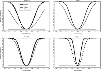
. We take T^X = T^Y = T^XY = 60 corresponding to 5 years of monthly data and φ = 0.5 throughout, while varying ρ ∈ {−0.9, 0, 0.5, 0.9}. The power curves for the 0.05 level two-sided tests are shown in Figure 1 calculated from 100,000 replications.

Power curves for the 0.05 level two-sided tests.

Throughout, the test based on τ_E has the higher power curve, but which test comes second changes according to the design: the common sample test does very poorly when ρ = −0.9, whereas the full sample test does very poorly when ρ = 0.9, as predicted by the theory. We acknowledge that the feasible version of τ_E can suffer from small sample effects that might diminish its edge, and we intend to investigate this in future work.

Finally, this estimation/testing strategy can also be applied to the c.d.f.s in Example 2. Specifically, define for each z the vector of sample moments

and define estimates

by the preceding minimum distance strategy. Then define

, which converges weakly under the null hypothesis to Δ_F^E = sup_z W_F^E(z), where W_F^E(·) is some Gaussian process. By construction

are more efficient than

, and it may be possible to show that tests based on δ^E are more powerful than those based on δ.

Suppose it can be shown that W_F(·) = W_F^E(·) + U(·), where U(·) is independent of W_F^E(·). If

were semiparametrically efficient, this structure would be expected by the Hajek–Le Cam convolution theorem (Bickel et al., 1993, p. 182). It follows that the critical value of the one-sided test based on

is smaller than that based on

(see Bickel et al., 1993, p. 194), and so the former test should be more powerful under local alternatives that shift the location of the limiting processes equally.

5. CONCLUDING REMARKS

We have shown how to modify inference procedures in some special unbalanced data cases. In particular, we showed how to conduct valid inference for the “natural” full sample test statistics τ,δ in our two examples. We also showed that these may not be the most powerful tests, and indeed there are situations where using only the common sample may be superior. We proposed more efficient tests that use all the data and require estimates of long-run variances to do the optimal weighting.

Our results can be generalized in a number of ways. First, in the multivariate case there is possibility for further efficiency/power improvements. Second, we can consider more general nonseparable hypotheses. For example, consider the hypothesis that E [a(X_t,Y_t,…,X_t−p,Y_t−p)] = 0 for some known function a and lag length p. This involves the joint distribution of (X_t,Y_t,…,X_t−p,Y_t−p), not just its marginals. Nevertheless, one can generally improve on the test statistic (T^XY)⁻¹ [sum ]_{t:t,…,t−p∈I^XY} a(X_t,Y_t,…,X_t−p,Y_t−p) using the minimum distance strategy discussed in Section 4 by taking appropriate choice of moments.