1 Introduction
1.1 Background
In contrast to indoor conditions that are controlled mechanically, naturally ventilated spaces surrender themselves to the forces and fluctuations of their surrounding environments (see, for example, Linden Reference Linden1999). In addition to the prediction of the steady state of a system, one should therefore be concerned with its robustness or its propensity to switch abruptly to an alternative steady state.
In the specific case of an indoor space subjected to a source of heating and an external wind load, the governing equations admit multiple steady-state solutions (Hunt & Linden Reference Hunt and Linden2005). The solutions correspond to either forward flow or reverse flow, for which unidirectional discharge occurs through the opening at the top or bottom of the space, respectively. From an operational point of view it is necessary to consider the transient route towards these steady states from time-dependent governing equations (Kaye & Hunt Reference Kaye and Hunt2004; Coomaraswamy & Caulfield Reference Coomaraswamy and Caulfield2011). The analysis of the system’s transient behaviour leads naturally to questions relating to the sensitivity and robustness of steady states to random or controlled variations in design or environmental conditions.
There exist reverse flows that are unstable, in the sense that infinitesimal changes in the wind’s strength will cause a dramatic change in the system’s state. In contrast, there exist locally stable reverse and forward flows that are insensitive to infinitesimal changes in the wind. Finite changes in the wind, however, can result in a transition between stable forward flow and stable reverse flow, and provide the motivation for the present study.
Previous work (Yuan & Glicksman Reference Yuan and Glicksman2008; Lishman & Woods Reference Lishman and Woods2009) has determined the minimum instantaneous amount by which the strength of an opposing wind must increase to force a transition from forward flow to reverse flow, under the assumption of a base state consisting of uniform buoyancy. Given that isolated sources of buoyancy and heterogeneous boundary conditions result in spatially non-uniform distributions of buoyancy (see, for example, Linden, Lane-Serff & Smeed Reference Linden, Lane-Serff and Smeed1990), we relax the assumption of uniform buoyancy and quantify the extent to which the destruction of a stratified interior modifies the system’s robustness to fluctuations in the wind.
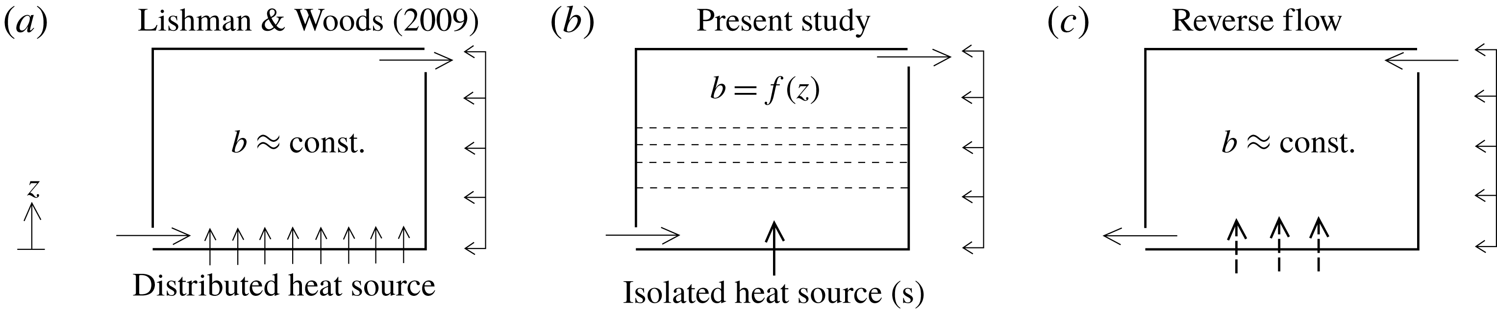
The ventilation driven by (a) a well-mixed interior of uniform buoyancy and (b) a stably stratified interior. (c) Schematic illustrating reverse flow, for which the interior is well-mixed and assumed to be of uniform buoyancy.

1.2 An illustration of the general problem
Consider a volume with low- and high-level openings, as depicted in figure 1. In figure 1(a), following Lishman & Woods (Reference Lishman and Woods2009), the heating of the space is distributed evenly over the floor and the resulting buoyancy field is assumed to be uniform. In figure 1(b), which is the starting point for the present work, the heating occurs unevenly over localised sources to produce a buoyancy field that is non-uniform (i.e. stratified). Ventilation of the space is driven by pressure differences resulting from the average internal buoyancy and external forces arising from the wind. In a steady state, the rate at which buoyancy drains from the top of the space is equal to the rate at which it is supplied to the space in the form of heat, which we assume to be the same in figure 1(a–c).
The average buoyancy and ventilation rate is greater in figure 1(a) than in figure 1(b) (see, for example, Gladstone & Woods Reference Gladstone and Woods2001, § 4.3). To understand why, note that the ventilation rate increases with pressure difference across the upper opening, which in turn increases with average buoyancy in the volume. For a given average buoyancy, the buoyancy at the top of the volume in figure 1(a) is less than it is for any stable stratification figure 1(b); hence the buoyancy flux through the upper opening will only be the same in both cases if the ventilation rate – and therefore the average buoyancy – is maximised in figure 1(a).
Figure 1(c) illustrates a situation in which the pressure difference across the space due to wind exceeds the pressure difference created by internal buoyancy. The resulting flow is in the reverse direction and is accompanied by an approximately well-mixed interior of uniform buoyancy, regardless of the way in which the space is heated (Hunt & Linden Reference Hunt and Linden2005). In a steady state, the average buoyancy in figure 1(c) is necessarily less than the average buoyancy in figure 1(b) and, therefore, less than the average buoyancy in figure 1(a).
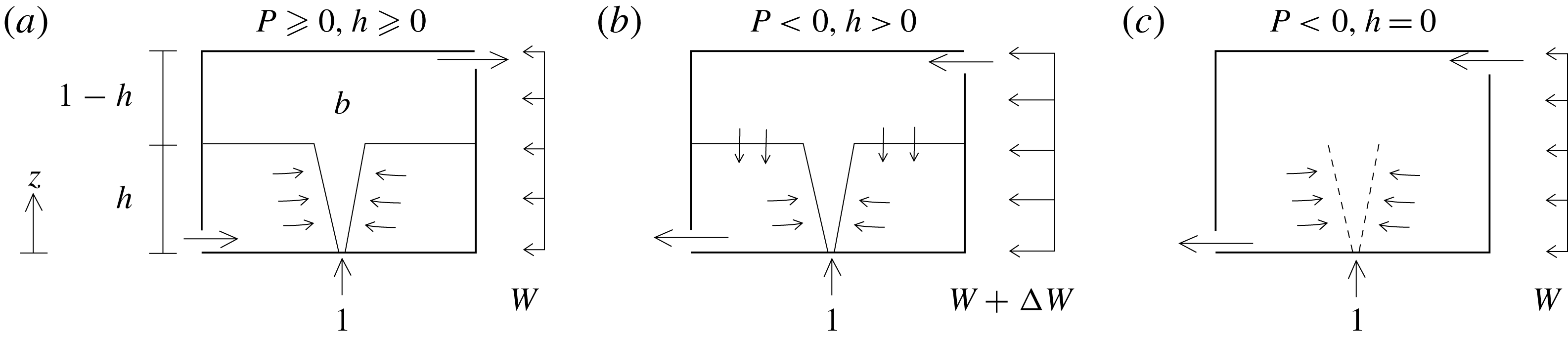
Wind-opposed buoyancy-driven ventilation resulting in (a) steady forward flow; (b) transient reverse flow with a stratification; and (c) steady reverse flow. A sufficiently large increase
 $\unicode[STIX]{x0394}W$
in the opposing wind
 $W$
results in a transition from (a) to (c).

A transient increase in the opposing wind strength can cause a transition from forward flow to reverse flow. The question that our work addresses is whether the minimum increase in the wind strength that is required for the transition is greater for the system in figure 1(a) than it is for the system in figure 1(b). Whilst the required reduction in average buoyancy is greater for the system in figure 1(a), we show that the wind must perform additional work over a finite time to destroy the stratification for the system in figure 1(b), making it more robust to fluctuations in the wind than one might otherwise expect.
1.3 Theoretical model
We will assume that buoyancy is introduced from a point source located at the bottom of a domain, whose ventilation is facilitated by low- and high-level openings. For forward flow, the resulting two-layer stratification, illustrated in figure 2(a), is a special example of the stratified environments that were considered in figure 1(b). The state of the system can be described by the dimensionless height of the resulting interface
 $h$
and the dimensionless uniform buoyancy
 $b$
of a well-mixed upper layer, which, following Coomaraswamy & Caulfield (Reference Coomaraswamy and Caulfield2011), are non-dimensionalised using the total domain height and plume buoyancy flux. Following Hunt & Linden (Reference Hunt and Linden2005), the volume flow rate through the space is determined by the dimensionless pressure difference
 $$\begin{eqnarray}P=\underbrace{b(1-h)}_{\mathit{buoyancy}}-\underbrace{W}_{\mathit{wind}},\end{eqnarray}$$
between the dimensionless stack-induced pressure difference
 $b(1-h)$
and the dimensionless wind-induced pressure difference
 $W$
between the windward and leeward openings, where
 $W$
corresponds to the square of a Froude number based on the wind speed. In adopting this notation, which differs slightly from the explicit use of the Froude number
 $Fr\propto \sqrt{W}$
by Hunt & Linden (Reference Hunt and Linden2005) to express the same physical concepts, we follow Coomaraswamy & Caulfield (Reference Coomaraswamy and Caulfield2011), in which further details pertaining to the non-dimensionalisation can be found.
In an unsteady state the governing equations comprise statements of volume conservation and buoyancy conservation in the upper layer:
 $$\begin{eqnarray}{\displaystyle \frac{\text{d}h}{\text{d}t}}=\left\{\begin{array}{@{}l@{}}-h^{5/3}+|VP|^{1/2},\quad \\ -h^{5/3}-|VP|^{1/2},\quad \\ 0,\quad \end{array}\right.\quad {\displaystyle \frac{\text{d}}{\text{d}t}}b(1-h)=\left\{\begin{array}{@{}ll@{}}1-|VP|^{1/2}b,\quad & P\geqslant 0,h\geqslant 0,\\ 1,\quad & P<0,h>0,\\ 1-|VP|^{1/2}b,\quad & P<0,h=0,\end{array}\right.\end{eqnarray}$$
respectively, where
 $V$
is a dimensionless opening area that accounts for discharge coefficients. The
 $h^{5/3}$
in (1.2a
) corresponds to the volume flux in an axisymmetric plume at
 $z=h$
, which would cause the height of the interface to reduce in the absence of the stack-driven discharge
 $|VP|^{1/2}$
. The subequations in (1.2) refer to forward displacement ventilation (
 $P\geqslant 0$
,
 $h\geqslant 0$
), reverse displacement ventilation (
 $P<0$
,
 $h>0$
) and reverse mixing ventilation (
 $P<0$
,
 $h=0$
), as depicted in figure 2. If a well-mixed interior of uniform buoyancy is assumed from the outset (as it is in Lishman & Woods Reference Lishman and Woods2009), the system’s state can be uniquely described by the buoyancy
 $b$
alone, which evolves according to (1.2b
) with
 $h=0$
.
When
 $W$
exceeds a critical value
 $W_{c}=\sqrt[3]{27/4V}$
, the system has three fixed points, at which
 $\text{d}(b,h)/\text{d}t=0$
, each corresponding to a different steady-state solution (Hunt & Linden Reference Hunt and Linden2005). For
 $W>W_{c}$
there are two stable solutions and an unstable steady-state solution describing reverse flow. Reverse flow is not possible when
 $W<W_{c}$
and, as pointed out by Lishman & Woods (Reference Lishman and Woods2009), stable reverse flow subjected to decreasing wind will jump to displacement ventilation when
 $W<W_{c}$
.
The fixed point for forward flow
 $(b_{0},h_{0})$
through a stratified environment satisfies (1.2) for
 $P\geqslant 0$
:
 $$\begin{eqnarray}b_{0}=h_{0}^{-5/3},\quad Vh_{0}^{-5/3}(1-h_{0})-h_{0}^{10/3}-VW=0.\end{eqnarray}$$
A fixed point for reverse flow when
 $W>W_{c}$
satisfies (1.2b
) for
 $h=0$
and is therefore a stable or unstable state corresponding to one of two positive real roots of the cubic
 $$\begin{eqnarray}b^{3}-Wb^{2}+V^{-1}=0.\end{eqnarray}$$
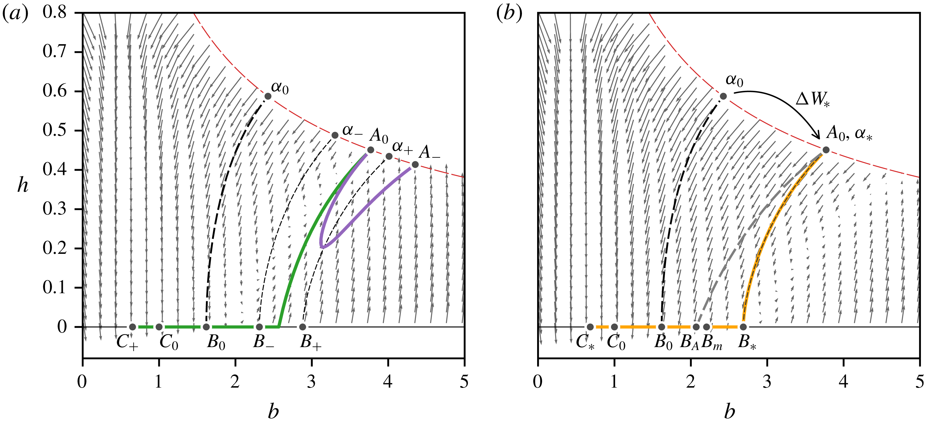
It is useful to regard the two-dimensional phase space for the system, shown in figure 3, as a projection of the space to which states
 $(b,h,W,V)$
belong. Constant values of
 $V$
and
 $W$
correspond to a particular plane or slice through the entire space. The features of phase space that are shown in the projection in figure 3 therefore depend on particular values of
 $V$
and
 $W$
, whose axes are hidden from view. Whilst the grey arrows in figure 3(a) correspond to the system’s time derivatives when
 $V=1$
and
 $W=2>W_{c}$
, we have also included the system’s trajectory for wind strengths
 $W+\unicode[STIX]{x0394}W$
to indicate how the system would evolve if the base wind strength
 $W$
were to change by
 $\unicode[STIX]{x0394}W$
.
As discussed in Coomaraswamy & Caulfield (Reference Coomaraswamy and Caulfield2011), states for which
 $h>b^{-3/5}$
, representing an upper layer whose buoyancy exceeds the buoyancy in the plume at the interface, are beyond the scope of the model equations and therefore not included in figure 3. For a given base wind strength
 $W\geqslant W_{c}$
, the phase space is partitioned by a separatrix curve
 $B_{0}{-}\unicode[STIX]{x1D6FC}_{0}$
, which emanates from the unstable fixed point
 $B_{0}$
, into basins of attraction corresponding to the stable fixed points
 $A_{0}$
and
 $C_{0}$
. The fixed point to which a system’s state eventually evolves is determined by whether its state lies to the left or to the right of the separatrix curve. The separatrix curve can be obtained by adding a small positive perturbation to
 $h=0$
at the unstable fixed point
 $B_{0}$
, to provide initial conditions for the integration of the governing equations backwards in time until
 $h=b^{-3/5}$
at
 $\unicode[STIX]{x1D6FC}_{0}$
.
The projected phase space for a two-layer stratification with base wind strength
 $W=2$
and
 $V=1$
. The points
 $A_{0}$
,
 $B_{0}$
and
 $C_{0}$
denote the stable (forward flow), unstable and stable (reverse flow) fixed points of the system, respectively. The line
 $\unicode[STIX]{x1D6FC}_{0}{-}B_{0}$
denotes the separatrix curve for
 $W=2$
and
 $V=1$
. The lines
 $A_{0}{-}A_{-}$
and
 $A_{0}{-}C_{+}$
in
 $(a)$
denote the trajectories taken by the system following suboptimal
 $\unicode[STIX]{x0394}W=0.5<\unicode[STIX]{x0394}W_{\ast }$
and superoptimal
 $\unicode[STIX]{x0394}W=1.0>\unicode[STIX]{x0394}W_{\ast }$
step changes in the wind strength, respectively. The thin dashed lines
 $\unicode[STIX]{x1D6FC}_{-}{-}B_{-}$
and
 $\unicode[STIX]{x1D6FC}_{+}{-}B_{+}$
denote the position of the separatrix curves for sub- and superoptimal changes in the wind, respectively. The line
 $A_{0}{-}C_{\ast }$
in
 $(b)$
denotes the trajectory taken by the system following an optimal
 $\unicode[STIX]{x0394}W_{\ast }\approx 0.825$
step change in the wind strength, which, for
 $h>0$
coincides with the system’s separatrix curve
 $\unicode[STIX]{x1D6FC}_{\ast }{-}B_{\ast }$
for the wind strength
 $W+\unicode[STIX]{x0394}W_{\ast }$
. Along
 $A_{0}{-}B_{A}$
the average buoyancy
 $b_{0}(1-h_{0})$
is constant and
 $B_{A}$
corresponds to the location of the unstable fixed point for a suboptimal step change
 $\unicode[STIX]{x0394}W<\unicode[STIX]{x0394}W_{\ast }$
in wind strength. The point
 $B_{m}$
is the location of the fixed point for forward flow, under the assumption of a well-mixed interior (Lishman & Woods Reference Lishman and Woods2009). The grey arrows denote the time derivatives of a given state
 $(b,h)$
for an opposing wind of strength
 $W$
in (a) and
 $W+\unicode[STIX]{x0394}W_{\ast }$
in (b).

2 Flow reversal
The direction of the flow through the system can be permanently reversed by a sustained increase
 $\unicode[STIX]{x0394}W$
in the wind strength. The resulting pressure difference must be larger than the favourable pressure difference created by the upper layer of warm fluid during the transition.
2.1 The critical change
 $\unicode[STIX]{x0394}W_{\ast }$
in the wind strength

If the system’s state starts at the fixed point
 $A_{0}$
corresponding to steady forward flow for a base wind strength
 $W$
, a step increase
 $\unicode[STIX]{x0394}W$
in the wind strength will cause the state to change. Hereafter we refer to
 $\unicode[STIX]{x0394}W_{\ast }$
as the minimum increase required to permanently reverse the flow. Thus, when
 $\unicode[STIX]{x0394}W<\unicode[STIX]{x0394}W_{\ast }$
, the system returns to a state corresponding to forward flow (see, for example, the line
 $A_{0}{-}A_{-}$
in figure 3
a, projected from the plane
 $W+\unicode[STIX]{x0394}W$
). When
 $\unicode[STIX]{x0394}W>\unicode[STIX]{x0394}W_{\ast }$
the system transitions to a state corresponding to stable reverse flow (see, for example, the line
 $A_{0}{-}C_{+}$
in figure 3
a, projected from the plane
 $W+\unicode[STIX]{x0394}W$
). Whether a transition to stable reverse flow occurs depends on whether the step increase
 $\unicode[STIX]{x0394}W$
moves the separatrix curve to the left or to the right of the system’s base state
 $A_{0}$
.
The strength of the optimal (minimum) wind increase
 $\unicode[STIX]{x0394}W_{\ast }:\unicode[STIX]{x1D6FC}_{0}\mapsto \unicode[STIX]{x1D6FC}_{\ast }$
projects the point
 $\unicode[STIX]{x1D6FC}_{\ast }$
of the separatrix curve in the
 $W+\unicode[STIX]{x0394}W_{\ast }$
plane exactly onto the fixed point
 $A_{0}$
for forward flow corresponding to
 $W$
, as shown in figure 3(b). The increase would need to be sustained for at least as long as it would take for the system’s trajectory to cross the separatrix curve at the unstable fixed point
 $B_{0}$
associated with the base wind strength
 $w$
. No instantaneous increase for which
 $\unicode[STIX]{x0394}W<\unicode[STIX]{x0394}W_{\ast }$
can reverse the flow because
 $\unicode[STIX]{x0394}W_{\ast }$
is the smallest step change that places the system’s state in the basin of attraction for stable reverse flow in the
 $W$
plane.
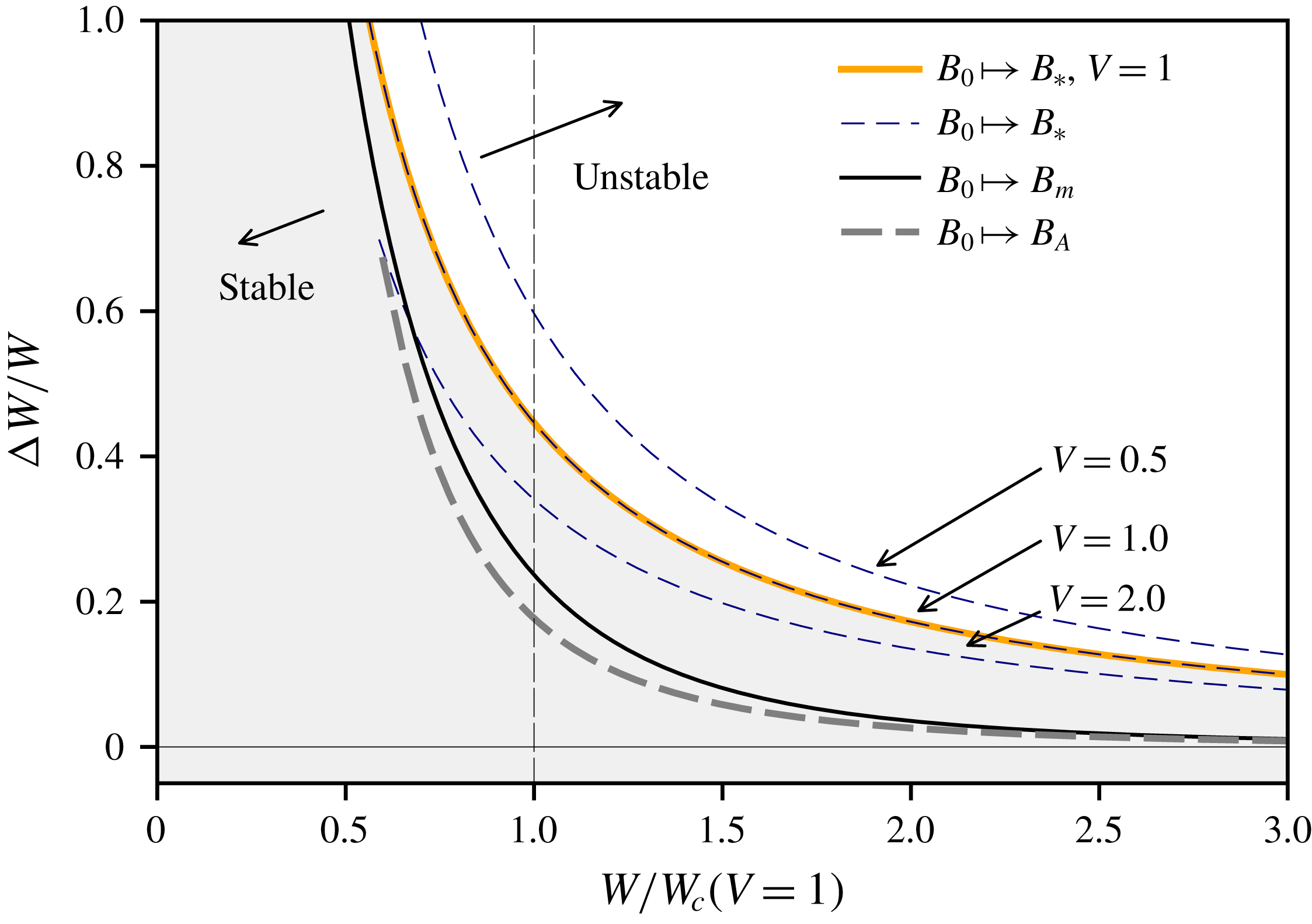
Stability diagram indicating instantaneous increases in the wind strength
 $\unicode[STIX]{x0394}W$
that cause a reversal of forward ventilation flow. The stable (shaded) and unstable (unshaded) regions are separated by the minimal instantaneous increase in wind strength
 $\unicode[STIX]{x0394}W_{\ast }:B_{0}\mapsto B_{\ast }$
that is necessary to permanently reverse the ventilation of a two-layer stratified interior for an opening parameter
 $V=1$
(the dashed lines corresponding to
 $V=0.5$
and
 $V=2.0$
are included for comparison). The lines in the stable region correspond to the unstratified interior of uniform buoyancy considered by Lishman & Woods (Reference Lishman and Woods2009), corresponding to
 $B_{m}$
in figure 3(b), and the wind increase estimated from the average buoyancy
 $b_{0}(1-h_{0})$
of a two-layer stratification, corresponding to
 $B_{A}$
in figure 3(b).

The base wind strength that corresponds to
 $W+\unicode[STIX]{x0394}W_{\ast }$
can be found by integrating the governing equations backwards in time along the separatrix curve
 $B_{\ast }{-}\unicode[STIX]{x1D6FC}_{\ast }$
from
 $(b,h)=(b_{\ast },0)$
for
 $W+\unicode[STIX]{x0394}W_{\ast }$
, where
 $b_{\ast }$
satisfies a modified version of (1.4):
 $$\begin{eqnarray}b_{\ast }^{3}-(W+\unicode[STIX]{x0394}W_{\ast })b_{\ast }^{2}+V^{-1}=0.\end{eqnarray}$$
The point
 $\unicode[STIX]{x1D6FC}_{\ast }$
, at which the resulting trajectory intersects the line
 $h=b^{-3/5}$
, corresponds to the steady-state solution
 $A_{0}$
for forward flow for a base wind strength
 $W$
. Performing the calculation for different values of
 $W+\unicode[STIX]{x0394}W_{\ast }$
provides the relationship between
 $W$
and
 $\unicode[STIX]{x0394}W_{\ast }$
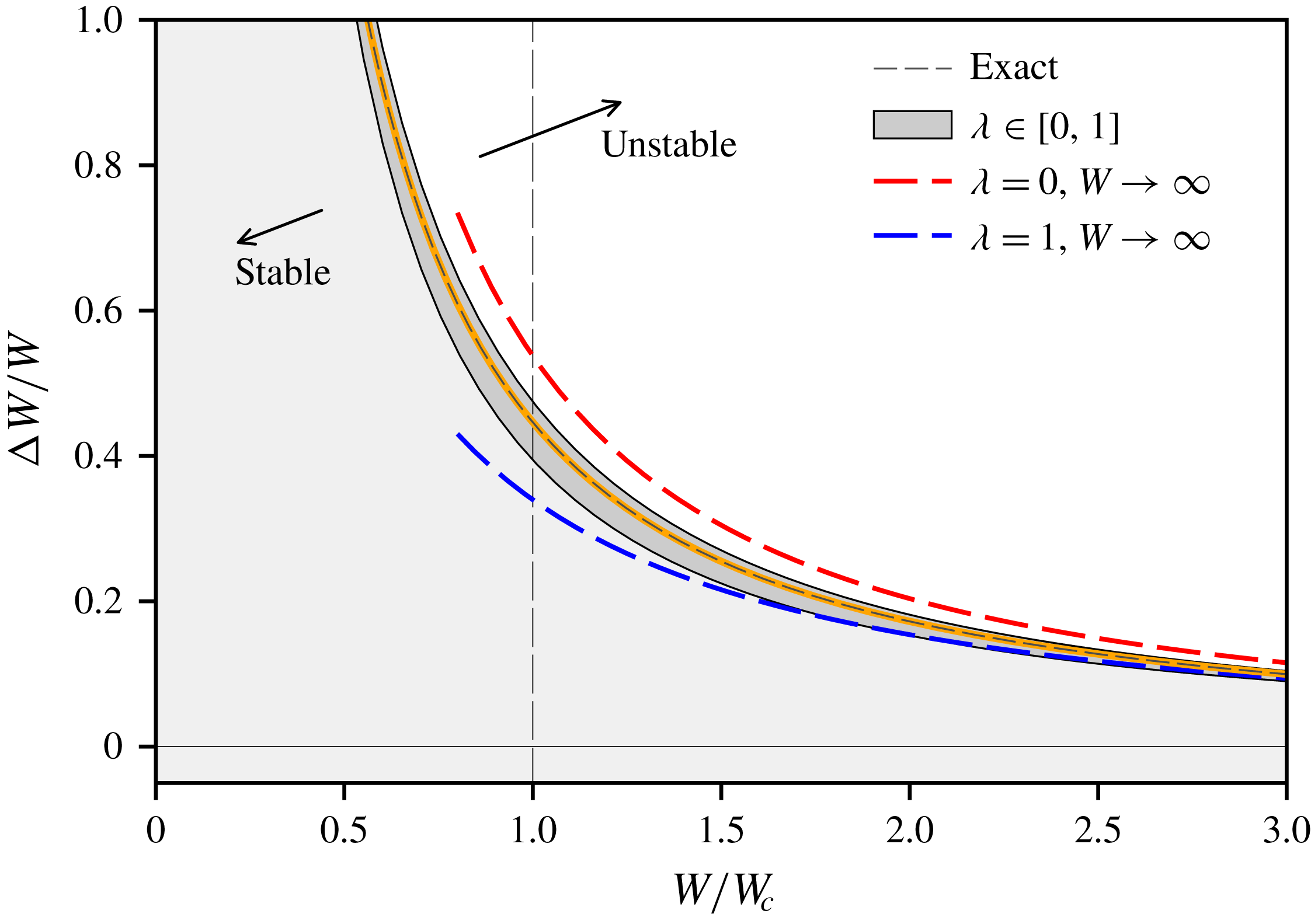
for marginal stability that is displayed in figure 4.
2.2 Comparison with Lishman & Woods (Reference Lishman and Woods2009)
A steady-state forward flow in the environment of uniform buoyancy considered by Lishman & Woods (Reference Lishman and Woods2009) satisfies (1.2b
) with
 $P\geqslant 0$
and
 $h=0$
:
 $$\begin{eqnarray}b_{m}^{3}-Wb_{m}^{2}-V^{-1}=0,\end{eqnarray}$$
whose real solution corresponds to
 $B_{m}$
in figure 3(b). It is evident from figure 3(b) that
 $b_{m}<b_{\ast }$
, where
 $b_{\ast }$
is the buoyancy of the stratified interior’s ‘upper’ layer when, during application of the step increase in the wind strength, the interface reaches floor level and the upper layer engulfs the entire space. The minimum increase in the wind necessary to reverse the flow through an initially stratified environment is therefore greater than it is for an environment whose buoyancy is initially uniform. As can be seen in figure 4, for base wind strengths close to
 $W_{c}=\sqrt[3]{27/4V}$
, the critical increase
 $\unicode[STIX]{x0394}W_{\ast }$
for a two-layer stratification is approximately twice as large as it is for an interior of uniform buoyancy, for which
 $\unicode[STIX]{x0394}W_{\ast }=2(b_{m}-W)$
(Lishman & Woods Reference Lishman and Woods2009). At larger base wind strengths
 $W\gg W_{c}$
a stratified interior can withstand changes in the wind that are an order of magnitude larger than those that can be withstood by an interior of uniform buoyancy.
We have demonstrated that states of uniform buoyancy satisfying (2.2) are less robust to changes in the wind than states consisting of a two-layer stratification satisfying (1.3). As explained in § 1.2, given that the average buoyancy of the two-layer stratification is less than the uniform buoyancy satisfying (2.2), we expect estimations of the system’s robustness based on its average buoyancy
 $b_{0}(1-h_{0})$
to be misleading and conservative. Indeed, as deduced in § 1.2, the line
 $A_{0}{-}B_{A}$
in figure 3(b), on which
 $b(1-h)=b_{0}(1-h_{0})$
is constant, intersects the horizontal axis
 $h=0$
at
 $B_{A}$
, where
 $b=b_{0}(1-h_{0})<b_{m}$
. Conclusions about the robustness of stratified environments based on their average buoyancy therefore provide a lower bound on the strength of the minimum destabilising increase in the wind, which suggests that the work required to homogenise a stratified interior plays a crucial role in determining its stability.
Changing the opening parameter
 $V$
affects neither the qualitative aspects of our results concerning the system’s robustness nor our comparisons with interiors of uniform buoyancy. As shown in figure 4, and consistent with intuition, large values of the opening parameter, corresponding to openings with relatively large area, make the stratified interior more susceptible to flow reversal, whilst small values make it more robust. It is interesting that the enhanced robustness afforded by a reduction in
 $V$
also entails a reduction in the height of the interface of a two-layer stratification.
Transient time scale associated with lowering the interface of a stratified interior along
 $A_{0}{-}B_{\ast }$
in figure 3 (
 $\unicode[STIX]{x0394}t_{\ast }$
, solved numerically) and purging relatively warm well-mixed air from the space along
 $B_{\ast }{-}C_{\ast }$
(
 $\unicode[STIX]{x0394}t_{0}$
, estimated using (2.4)) for an opening parameter
 $V=1$
. The curve labelled ‘
 $B_{m}{-}$
’ corresponds to the time scale estimated from (2.4) for a well-mixed state to move from
 $B_{m}$
to stable reverse flow. The thin dashed lines, whose gradients are
 $-1/2$
and
 $-2/5$
correspond to the asymptotic scaling of
 $\unicode[STIX]{x0394}t_{\ast }$
and
 $\unicode[STIX]{x0394}t_{0}$
when
 $W\rightarrow \infty$
, as discussed in § 3.

2.3 Time scale
The transient route that forward displacement flow takes before being permanently reversed by a sufficiently large increase
 $\unicode[STIX]{x0394}W_{\ast }$
in the wind strength comprises two distinct processes. The first involves lowering the interface of the stratification until the warm upper layer engulfs the entire space (
 $A_{0}{-}B_{\ast }$
in figure 3). The second involves purging warm air from the space via the lower opening until the system reaches stable equilibrium (
 $B_{\ast }{-}C_{\ast }$
in figure 3). The subject of this section is the time scale on which these processes occur.
The time
 $\unicode[STIX]{x0394}t_{\ast }$
that it takes for the interface to be lowered to floor level can be obtained by numerical integration, backwards in time, along
 $B_{\ast }{-}A_{0}$
, and is displayed in figure 5. A consequence of the discontinuity at
 $h=0$
in the governing equations (1.2) is that the time derivatives of
 $b$
and
 $h$
are non-zero arbitrarily close to the unstable fixed point
 $B_{\ast }$
. Physically, this corresponds to the fact that the interface descends with a finite speed just before it reaches floor level.
In contrast to the trajectory
 $A_{0}{-}B_{\ast }$
, temporal derivatives tend to zero at both ends of the trajectory
 $B_{\ast }{-}C_{\ast }$
, which makes the time scale associated with the purging of warm air from the space infinite without a perturbation at
 $B_{\ast }$
. Using (1.2) when
 $P<0$
,
 $h=0$
, for the modified wind strength
 $W+\unicode[STIX]{x0394}W_{\ast }$
, we define a characteristic time scale by noting that
 $-\text{d}b/\text{d}t$
is maximised when
 $b=2(W+\unicode[STIX]{x0394}W_{\ast })/3$
; hence
 $$\begin{eqnarray}-\frac{\text{d}b}{\text{d}t}\leqslant \left(\frac{W+\unicode[STIX]{x0394}W_{\ast }}{W_{c}}\right)^{3/2}-1,\end{eqnarray}$$
along
 $B_{\ast }{-}C_{\ast }$
. A useful lower bound on the time
 $\unicode[STIX]{x0394}t_{0}$
that it takes for the system to travel along
 $B_{\ast }{-}C_{\ast }$
is therefore
 $$\begin{eqnarray}\frac{\unicode[STIX]{x0394}b}{\left({\displaystyle \frac{W+\unicode[STIX]{x0394}W_{\ast }}{W_{c}}}\right)^{3/2}-1}\leqslant \unicode[STIX]{x0394}t_{0},\end{eqnarray}$$
where
 $\unicode[STIX]{x0394}b\geqslant 0$
is the difference in buoyancy between the two fixed points for reverse flow from (1.4). The time scale
 $\unicode[STIX]{x0394}t_{0}$
is displayed in figure 5 for
 $V=1$
, along with the total time
 $\unicode[STIX]{x0394}t_{\ast }+\unicode[STIX]{x0394}t_{0}$
. Note that the estimation (2.4) relates to the time taken for the system to reach
 $C_{\ast }$
, and does not, therefore, necessarily provide an indication of the minimum duration for which the increase in wind strength
 $\unicode[STIX]{x0394}W_{\ast }$
would be need to be sustained. The latter would involve estimating the time it would take for the system to travel along
 $B_{\ast }{-}B_{0}$
.
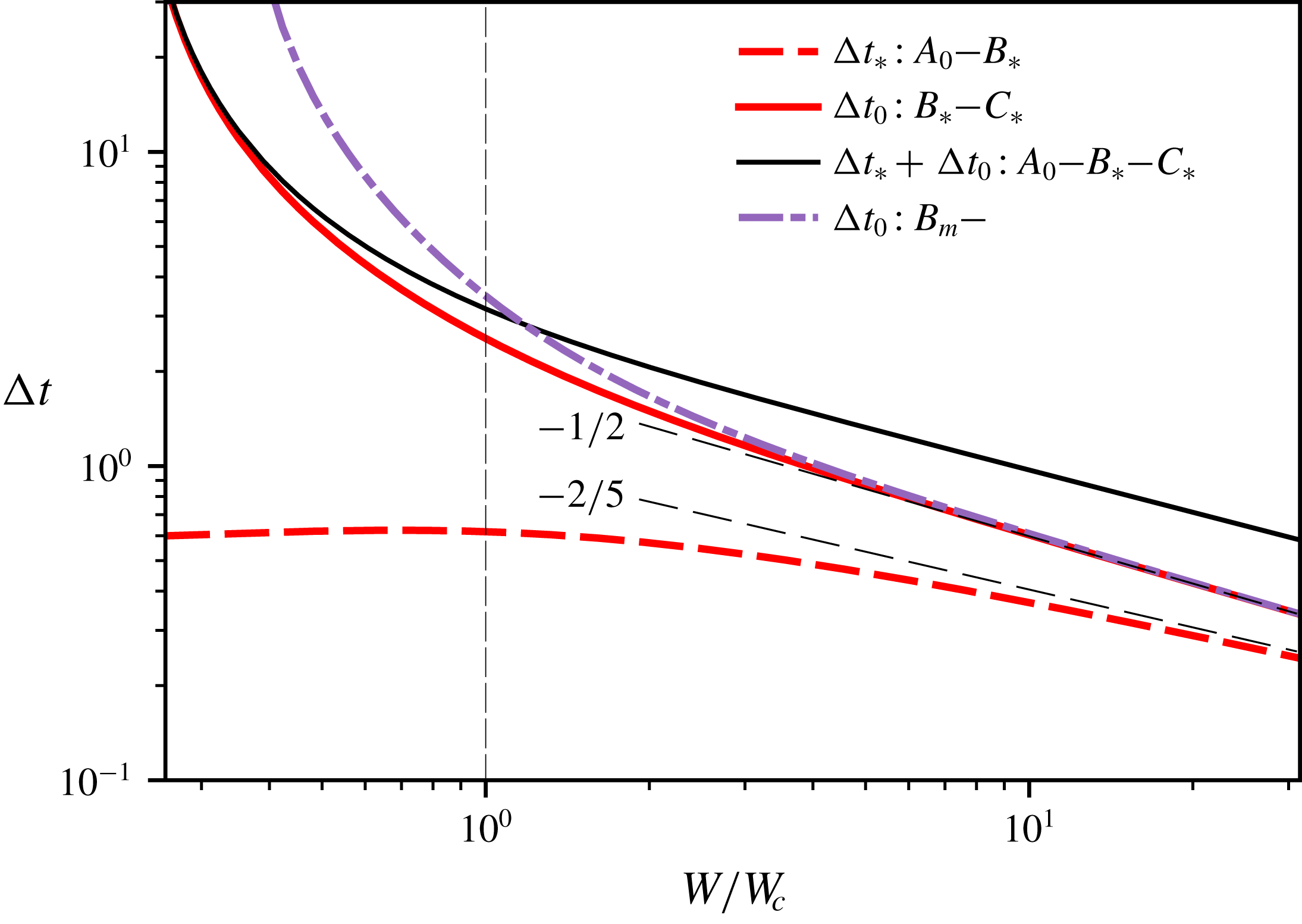
The lower bound (2.4) indicates that the time
 $\unicode[STIX]{x0394}t_{0}$
that it takes for the system to travel along
 $B_{\ast }{-}C_{\ast }$
is substantially larger than the time
 $\unicode[STIX]{x0394}t_{\ast }$
that it takes for the system to travel along
 $A_{0}{-}B_{\ast }$
, for the base wind speeds shown in figure 5. Both
 $\unicode[STIX]{x0394}t_{\ast }$
and
 $\unicode[STIX]{x0394}t_{0}$
decrease with increasing base wind strength
 $W$
. Consequently, the estimation (2.4) for a well-mixed interior, for which
 $\unicode[STIX]{x0394}W_{\ast }$
is less than it is for a stratified interior, is always greater than
 $\unicode[STIX]{x0394}t_{0}$
for a stratified interior, although the difference is insignificant for
 $W/W_{c}\gtrapprox 2$
.
To interpret figure 5 from a practical perspective it is useful to note that time in (1.2) is non-dimensionalised using the ‘filling box’ time scale (Coomaraswamy & Caulfield Reference Coomaraswamy and Caulfield2011)
 $S/(cF^{1/3}H^{2/3})$
, where
 $S$
is the horizontal area of the space,
 $c=6\unicode[STIX]{x1D700}/5(9\unicode[STIX]{x1D700}\unicode[STIX]{x03C0}^{2}/10)^{1/3}$
for an entrainment coefficient
 $\unicode[STIX]{x1D700}$
,
 $F$
is the buoyancy flux and
 $H$
is the height of the space. For reference, if
 $S=100~\text{m}^{2}$
,
 $F=0.1~\text{m}^{4}~\text{s}^{-3}$
(corresponding to a heat load of approximately 3.5 kW),
 $H=5~\text{m}$
and
 $\unicode[STIX]{x1D700}=0.1$
, the filling box time is approximately ten minutes. With this information in mind,
 $\unicode[STIX]{x0394}W_{\ast }$
can only be regarded as a ‘gust’ in the wind for sufficiently small filling box time scales or sufficiently large base wind speeds. It is otherwise more appropriate to regard
 $\unicode[STIX]{x0394}W_{\ast }$
as arising from a more persistent change in prevailing wind conditions.
3 Bounds on the stability of forward flow
3.1 Exact bounds
To understand the physics and scaling laws behind the stability of forward flow, we consider the trajectory that the system takes through phase space when it is subjected to an optimal increase in wind strength
 $\unicode[STIX]{x0394}W_{\ast }$
. Rather than retaining the volume flux
 $h^{5/3}$
in (1.2a
), which depends on the unknown and variable interface height
 $h$
, we assume the volume flux to be equal to the constant
 $\unicode[STIX]{x1D706}h_{0}^{5/3}$
, where
 $h_{0}$
is the initial interface height. Incorporation of the volume flux in this way results in a tractable differential equation and facilitates the over and under estimation of the effect that the plume’s volume flux has on the system’s stability. By substituting the solution
 $b(1-h)=b_{\ast }+t$
of (1.2b
) for
 $P<0,h>0$
into the modified (1.2a
) using the buoyancy
 $b_{\ast }$
at the unstable fixed point, one obtains
 $$\begin{eqnarray}{\displaystyle \frac{\text{d}h}{\text{d}t}}=-\unicode[STIX]{x1D706}h_{0}^{5/3}-V^{1/2}(W+\unicode[STIX]{x0394}W_{\ast }-b_{\ast }-t)^{1/2}.\end{eqnarray}$$
Along the separatrix curve,
 $h$
varies monotonically between
 $h_{0}$
and 0, which means that (3.1) with
 $\unicode[STIX]{x1D706}\in [0,1]$
bounds the actual solution to (1.2a
). Noting that the system is to be integrated backwards in time from
 $(b_{\ast },0)$
,
 $\unicode[STIX]{x1D706}=0$
corresponds to neglecting the volume flux in the plume, underestimating the ascent rate of the interface and overestimating the optimal change in wind strength
 $\unicode[STIX]{x0394}W_{\ast }$
. Conversely,
 $\unicode[STIX]{x1D706}=1$
corresponds to overestimating the volume flux in the plume, overestimating the ascent rate of the interface and underestimating the optimal change in wind strength
 $\unicode[STIX]{x0394}W_{\ast }$
. In either case, (3.1) provides a good approximation for the small interface heights that occur for large
 $W$
, because they entail a relatively small volume flux term.
Upper and lower bounds of the optimal wind increase
 $\unicode[STIX]{x0394}W_{\ast }$
, indicated by the dark grey region in the vicinity of the marginal stability curve (thin dashed line). The long dashed lines
 $\unicode[STIX]{x1D706}=0$
and
 $\unicode[STIX]{x1D706}=1$
correspond to asymptotic expressions for the upper and lower bounds, respectively, from (3.7).

Unlike the original differential equation, equation (3.1) is readily solved analytically to give
 $$\begin{eqnarray}h_{0}=\unicode[STIX]{x1D706}h_{0}^{5/3}\unicode[STIX]{x0394}t_{\ast }+\frac{2V^{1/2}}{3}(W+\unicode[STIX]{x0394}W_{\ast }-b_{\ast }+t)^{3/2}|_{0}^{\unicode[STIX]{x0394}t_{\ast }},\end{eqnarray}$$
where
 $\unicode[STIX]{x0394}t_{\ast }=b_{\ast }-b_{0}(1-h_{0})$
is the time it takes the system to reach the unstable fixed point. Equation (3.2) provides the algebraic bounds of the shaded region displayed in figure 6, which exhibits a close agreement with the exact curve for the system’s marginal stability, illustrating that the volume flux does not play a significant role in determining the system’s stability.
3.2 Asymptotic scaling for
$W\rightarrow \infty$

For forward flow (1.3) implies that the buoyancy and interface height at the stable fixed point are, respectively:
 $$\begin{eqnarray}b_{0}=W+W^{2/5}+O\left(\frac{1}{W^{1/5}}\right),\quad h_{0}=\frac{1}{W^{3/5}}-\frac{3}{5}\frac{1}{W^{6/5}}+O\left(\frac{1}{W^{9/5}}\right),\end{eqnarray}$$
for fixed
 $V$
, which implies that the total buoyancy of the upper layer at the stable fixed point scales according to
 $$\begin{eqnarray}b_{0}(1-h_{0})=W+\frac{1}{VW^{2}}+O\left(\frac{1}{W^{13/5}}\right).\end{eqnarray}$$
As
 $W\rightarrow \infty$
the stable interface height
 $h_{0}\rightarrow 0$
and (2.2), describing the well-mixed interior assumed by Lishman & Woods (Reference Lishman and Woods2009), indicates that, to leading order, the buoyancy of the stable fixed point for forward flow in a well-mixed interior scales in the same way as
 $b_{0}(1-h_{0})$
:
 $$\begin{eqnarray}b_{m}=W+\frac{1}{VW^{2}}+O\left(\frac{1}{W^{5}}\right).\end{eqnarray}$$
From (2.1), the buoyancy at the unstable fixed point
 $B_{\ast }$
for reverse flow at wind strength
 $W+\unicode[STIX]{x0394}W_{\ast }$
, assuming that
 $\unicode[STIX]{x0394}W_{\ast }=o(W)$
, is:
 $$\begin{eqnarray}b_{\ast }\sim W+\unicode[STIX]{x0394}W_{\ast }-\frac{1}{VW^{2}}.\end{eqnarray}$$
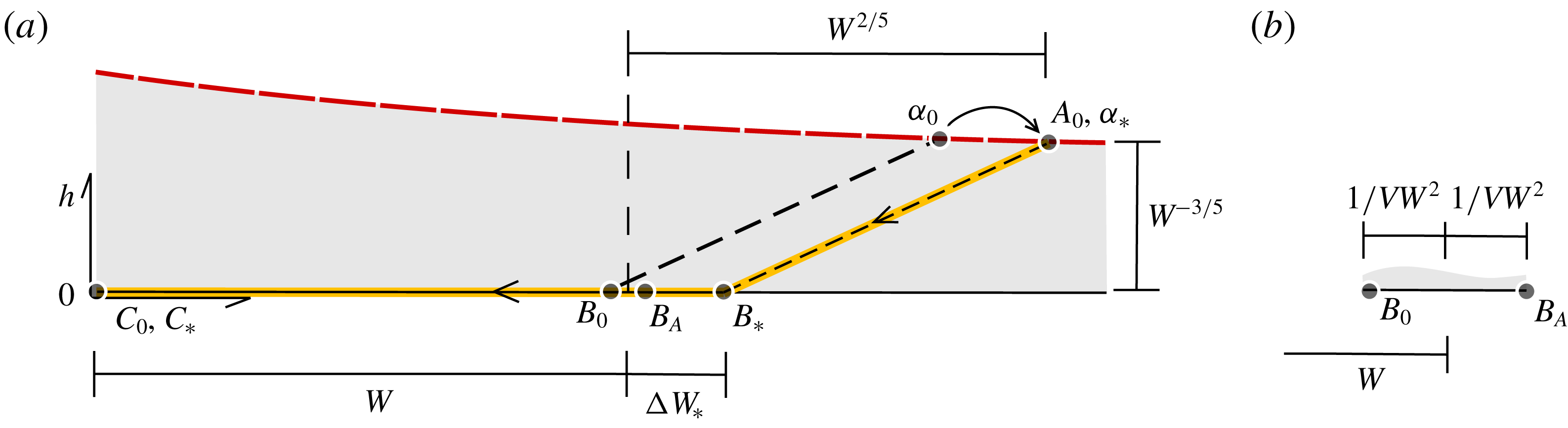
Figure 7 illustrates the scaling of the features of phase space when
 $W\rightarrow \infty$
. The interface height is small in comparison with the distance between the stable fixed points for forward and reverse flow. Note that
 $b\sim 1/\sqrt{VW}\rightarrow 0$
is a solution to (1.4) for
 $W\rightarrow \infty$
and corresponds to a stable reverse flow in which the interior is rapidly flushed by the wind. In order to destabilise forward flow, the buoyancy associated with the unstable fixed point must increase by at least
 $\unicode[STIX]{x0394}W_{\ast }$
, whose scaling with respect to
 $W$
we determine below. Recalling that
 $\unicode[STIX]{x0394}t_{\ast }=b_{\ast }-b_{0}(1-h_{0})$
from buoyancy conservation, equations (3.4) and (3.6) imply that
 $\unicode[STIX]{x0394}t_{\ast }\sim \unicode[STIX]{x0394}W_{\ast }$
, which, on substitution into (3.2) with (3.3), gives
 $$\begin{eqnarray}\frac{2V^{1/2}}{3}\unicode[STIX]{x0394}W_{\ast }^{3/2}+\unicode[STIX]{x1D706}\frac{\unicode[STIX]{x0394}W_{\ast }}{W}-\frac{1}{W^{3/5}}\sim 0,\end{eqnarray}$$
which is a cubic in
 $\sqrt{\unicode[STIX]{x0394}W_{\ast }}$
for any given
 $\unicode[STIX]{x1D706}\in [0,1]$
. As indicated in figure 6, equation (3.7) provides a close agreement with the exact bounds obtained in the previous section, even for relatively small values of
 $W$
. In particular, when
 $\unicode[STIX]{x1D706}=0$
, (3.7) provides the useful upper bound:
 $$\begin{eqnarray}\unicode[STIX]{x0394}W_{\ast }\sim \left(\frac{3}{2}\right)^{2/3}\frac{1}{V^{1/3}W^{2/5}}.\end{eqnarray}$$
More generally, all solutions to (3.7) scale according to
 $\unicode[STIX]{x0394}W_{\ast }=O(1/W^{2/5})$
, which is significantly weaker than the scaling
 $\unicode[STIX]{x0394}W_{\ast }\sim 1/VW^{2}$
that is implied by (3.4)–(3.6), based on the assumption of a well-mixed interior driven by distributed heating (Lishman & Woods Reference Lishman and Woods2009), or a conserved average buoyancy in the case of localised heating.
The asymptotic representation of phase space (cf. figure 3
b) for
 $W\rightarrow \infty$
, where (a) depicts the region traversed by the system’s trajectory and (b) depicts the relatively small distance between the original unstable fixed point
 $B_{0}$
and the average buoyancy
 $B_{A}$
.

The asymptotic time scale
 $\unicode[STIX]{x0394}t_{\ast }\sim \unicode[STIX]{x0394}W_{\ast }$
using (3.8) is included in figure 5 alongside the lower-bound scaling
 $\unicode[STIX]{x0394}t_{0}\sim \sqrt{W_{c}^{3}/W}$
using
 $\unicode[STIX]{x0394}b\sim W$
in (2.4).
4 Energetics for
$W\rightarrow \infty$

We will now demonstrate that the scaling (3.8) accounts for the work performed by the wind to homogenise the interior. The optimal increase in wind strength
 $\unicode[STIX]{x0394}W_{\ast }$
instantaneously reverses the flow. Therefore, over the finite time it takes for the interface to be lowered from
 $h_{0}\ll 1$
to zero, the change in potential energy
 $\unicode[STIX]{x0394}E_{p}$
is:
 $$\begin{eqnarray}\unicode[STIX]{x0394}E_{p}=\frac{b_{0}(1-h_{0})h_{0}}{2}-\frac{\unicode[STIX]{x0394}t_{\ast }}{2}\sim \frac{W^{2/5}}{2}.\end{eqnarray}$$
The first term on the right-hand side of (4.1) accounts for lowering the centre of mass of the average buoyancy
 $b_{0}(1-h_{0})$
by
 $h_{0}/2$
, while the second term accounts for buoyancy added (uniformly) to the domain over
 $\unicode[STIX]{x0394}t_{\ast }\sim \unicode[STIX]{x0394}W_{\ast }\propto W^{-2/5}$
at an average height of
 $1/2$
, which is comparatively small.
Neglecting the
 $O(\unicode[STIX]{x0394}t_{\ast }h_{0})$
work performed by buoyancy in the lower layer, the change in the system’s potential energy is equal to a fraction
 $\unicode[STIX]{x1D702}\in [0,1]$
of the total work
 $\unicode[STIX]{x0394}E_{w}$
undertaken by the wind. To leading order, the pressure due to the wind is the base wind strength
 $W$
and the rate at which the wind performs work on the system corresponds to the product of pressure and volume flux. But, the integral of the volume flux over
 $\unicode[STIX]{x0394}t_{\ast }$
is simply the first term in (3.7), which corresponds to the last term in (3.1) and (3.2):
 $$\begin{eqnarray}\unicode[STIX]{x0394}E_{w}=\underbrace{W}_{\mathit{pressure}}\underbrace{\frac{2V^{1/2}}{3}\unicode[STIX]{x0394}W_{\ast }^{3/2}}_{\mathit{volume}}.\end{eqnarray}$$
Equating
 $\unicode[STIX]{x1D702}\unicode[STIX]{x0394}E_{w}$
with
 $\unicode[STIX]{x0394}E_{p}$
implies that
 $$\begin{eqnarray}\unicode[STIX]{x0394}W_{\ast }\sim \left(\frac{3}{4\unicode[STIX]{x1D702}}\right)^{2/3}\frac{1}{V^{1/3}W^{2/5}},\end{eqnarray}$$
for
 $W\rightarrow \infty$
, which is identical to (3.8) when
 $\unicode[STIX]{x1D702}=1/2$
. The fraction
 $\unicode[STIX]{x1D702}=1/2$
corresponds to the mixing efficiency of high-Rayleigh-number convection resulting from heating and cooling at the bottom and top of a domain, respectively (see, for example, Hughes, Gayen & Griffiths (Reference Hughes, Gayen and Griffiths2013) for the particular case of Rayleigh–Bénard convection).
5 Conclusions
The transient response of a stratified interior to sudden changes in the strength of the wind plays a significant role in determining a system’s robustness. In particular, the energy required to homogenise a stratified interior makes existing stability estimations based exclusively on a space’s average buoyancy overly conservative, especially in the case of large opposing wind strengths.
Two- or multiple-layer stratifications can be produced by a variety of localised sources of buoyancy, besides the point sources considered here. Each would entail a slightly different set of dynamical equations to account for the driven flow’s vertical variation in volume flux (see, for example, line plumes in Kaye & Hunt Reference Kaye and Hunt2004). However, our results are general in suggesting that for moderate to large base wind strengths it is the initial, steady-state, density profile that is dominant in determining the system’s robustness, rather than the particular contribution of volume and heat to the upper layers during the relatively rapid destruction of the stratification.
Further considerations are required to quantify the robustness of a given state more precisely. For example, a low-level opening of finite vertical extent is likely to erode the criterion for stability that we have developed by permitting buoyancy to escape from the interior before the interface reaches floor level (see, for example, Hunt & Linden Reference Hunt and Linden2005). On the other hand, the model that we have used assumes that fluid entering the upper layer mixes with the surrounding fluid completely and instantaneously. If relatively cool, dense air descended through the space without mixing significantly with the upper layer, the interface would not be lowered and the critical increase in wind strength might be even larger than our predictions suggest. Whilst such effects are captured phenomenologically by values of
 $\unicode[STIX]{x1D702}$
in (4.3) that are less than
 $1/2$
, they warrant further attention.
Acknowledgement
J.C. gratefully acknowledges an Imperial College Junior Research Fellowship.