2.1. Experimental procedure

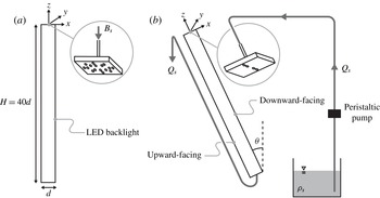
We conduct our buoyancy-induced turbulent mixing experiments in a long narrow tank that is inclined at an angle ${\it\theta}$ from the vertical and has dimensions $d\times d\times H$ , where $H=40d$ and $d=0.05~\text{m}$ . The tank is mounted on an axle which can be locked at the desired angle ${\it\theta}$ , and in order to ensure that the angle of tilt, ${\it\theta}$ , is precise, we use a plumb-bob and measure the tilt angle relative to this vertical. We fix our coordinate system to the middle of the top front edge of the tank, as shown in figure 1, such that the width of the tank lies in $x\in [-d/2,d/2]$ , the length of the tank lies in $z\in [-40d,0]$ and the extent of the tank in the line-of-sight direction lies in $y\in [0,d]$ . We refer to the boundary at $x=d/2$ as the ‘downward-facing’ boundary and the boundary at $x=-d/2$ as the ‘upward-facing’ boundary, as marked in figure 1. Initially, the tank is slowly filled with fresh clear water of density ${\it\rho}_{0}$ , while ensuring that no bubbles (which may interfere with our image analysis method, discussed in § 2.2) adhere to the sides of the tank.

Figure 1.

Schematic overview of the long narrow tank of dimensions $d\times d\times H$ ; (a) and (b) show the tank when it is vertical and when it is inclined at an angle ${\it\theta}$ from the vertical respectively. A buoyancy flux $B_{s}$ of salty dyed fluid of density ${\it\rho}_{s}$ is introduced at the top of the tank at $z=0$ with a peristaltic pump, which pumps the salty dyed fluid at a volume flow rate $Q_{s}$ from a reservoir. Insets show the manifold that is used in order to assist in diffusing momentum; the holes located in $x<0$ are plugged when ${\it\theta}>0^{\circ }$ to prevent fluid from solely being introduced at $x=-d/2$ . To conserve volume in the tank, a long tube is connected at the bottom of the tank, $z=-40d$ , and is held at the free surface of the fluid in the tank at $z=0$ , so that the height of the free surface of the fluid in the tank remains stationary throughout an experiment.

During an experiment, a peristaltic pump provides a constant volume flow rate $Q_{s}$ of dense saline source fluid of density ${\it\rho}_{s}>{\it\rho}_{0}$ at the top of the tank at $z=0$ . The dense source fluid is fed through a tube into a manifold of width $d$ with many holes spread out over its cross-section at its outlet. For experiments with a tilt angle of ${\it\theta}=0^{\circ }$ , the dense source fluid drips out of the many holes of the manifold into the fresh clear water at random positions over the cross-section of the tank. This is done to minimise the momentum of the dense source fluid so that we can assume this injection of dense source fluid to be a pure source of buoyancy. However, for tilt angles ${\it\theta}>0^{\circ }$ , the dense source fluid is forced to flow out of the holes positioned at $x=0$ by plugging the holes in the manifold at $x<0$ . This is done so that the dense source fluid initially descends as a plume and becomes fully mixed with the ambient fluid across the width of the tank over an along-tank length scale of $O(5d)$ , as also described by VS12. We note that experiments with ${\it\theta}=0^{\circ }$ where all of the holes were plugged except for those positioned at $x=0$ were also conducted. These experiments yielded results that were similar to those obtained without the holes plugged. Therefore, we believe that the exact details of the source are unimportant to the subsequent evolution of the flow. Finally, in order to conserve volume in the tank, a long tube is connected at the bottom of the tank, $z=-40d$ , and is held at the free surface of the fluid in the tank at $z=0$ , so that the height of the free surface of the fluid in the tank remains stationary throughout an experiment.

As the dense source fluid is injected, it immediately begins to mix with the fresh clear water. Therefore, in general, the density ${\it\rho}$ in the tank is in the range ${\it\rho}_{0}\leqslant {\it\rho}\leqslant {\it\rho}_{s}$ . We define the reduced gravity of the fluid in the tank, i.e. the downward acceleration of the mixed fluid assuming the Boussinesq approximation, to be

where $g$ is the acceleration due to gravity. In this paper, we focus on flows driven by an unstable density gradient, $(\partial g^{\prime }/\partial z)>0$ . The flow is thus driven by a constant source buoyancy flux $B_{s}=g_{s}^{\prime }Q_{s}$ introduced at $z=0$ which is given by

As in VS12, we introduce the dimensionless time scale

During an experiment, the dense source fluid mixes into the fresh clear water, and a region of mixed fluid propagates towards the bottom of the tank. In this paper, we restrict our attention to the dynamics of the flow for those times earlier than that at which mixed fluid is first detected at the bottom of the tank, i.e. the ‘initial mixing phase’ of VS12. Therefore, we define the start of an experiment $\tilde{t}=0$ as the moment when the pump begins to introduce the dense source fluid to the top of the tank and the end of an experiment $\tilde{t}=\tilde{t}_{f}$ as the moment when dyed fluid is first detected at the bottom of the tank.

2.2. Image analysis method

Our image analysis technique is similar to that used by VS12 (a detailed description is presented in Lin Reference Lin2014). The experimental tank is illuminated from behind with an LED backlight (Electroluminescent LightTape, Electro-LuminX Lighting Corp.) that provides approximately uniform illumination. The dense source fluid is dyed with dark red food dye (a ‘Preema’ product), and this dye acts as a tracer for the evolution of the turbulent mixing of the salty fluid and attenuates the light emitted by the backlight. We capture images of the line-of-sight light intensity of the flow $\langle I\rangle _{y}(x,z,t)$ , and divide the tank into a grid of $35\times 400$ cells. In each cell, we apply an independent calibration procedure to map $\langle I\rangle _{y}$ to the line-of-sight reduced gravity $\langle g^{\prime }\rangle _{y}=g^{\prime }$ of the mixed fluid within the tank as it evolves in time. Henceforth, we drop the brackets $\langle -\rangle _{y}$ denoting line-of-sight for convenience. We take pictures at a rate of 2 Hz with a Nikon D90 DSLR fitted with a Nikkor 18–135 mm $f/3.5$ –5.6 lens. For all experiments, the ISO is set to 200, the shutter speed is $1/200~\text{s}$ , the aperture is set to an $f$ -number of $f/5$ , the lens focal length is set to 50 mm and the colour temperature is held constant. We select this exposure in order to minimise noise and obtain clear images of the turbulent flow with minimal motion blur. This provides us with sufficient contrast in each image so that different concentrations of dye attenuated by the backlight are clearly detectable.

We define the cross-tank averaged reduced gravity $\overline{g^{\prime }}(z,t)$ as

Furthermore, we note that the spatially integrated reduced gravity within the tank is always balanced by the dense source fluid added,

In this way, we may check the precision of our image analysis method quantitatively. We find that the spatially integrated cross-tank averaged reduced gravity typically differs from the known amount of dense source fluid injected at $z=0$ by an amount less than 5 %. We believe that this is due to a combination of imprecisions of the pump, parallax errors and image distortion resulting from our lens. Furthermore, a range of grid sizes was explored, from $1\times 15$ cells to a pixel-by-pixel calibration, and the grid size used in this paper ( $35\times 400$ cells) was observed to be fine enough both to capture the details of the flow and minimise the error in satisfying (2.5).

2.3. Experimental parameters

Each of our experiments is characterised by three parameters: the tilt angle ${\it\theta}$ , the tank width $d$ and the injected buoyancy flux $B_{s}$ . Tilt angles from 0° to 30° were tested in $2.5^{\circ }$ increments, along with the tilt angles 35°, 40° and 45°. Based on dimensional analysis, we expect the flow speed to scale as $(B_{s}\cos {\it\theta})^{1/3}d^{-1/3}$ with a length scale $d$ , so we define the characteristic Reynolds number for this flow (after the mixed fluid is constrained by the width of the tank) as

where ${\it\nu}$ is the kinematic viscosity, and the buoyancy flux is multiplied by $\cos {\it\theta}$ in order to capture the effect of the component of gravity along the length of the tank. As the tank is tilted, the component of gravity available to drive the buoyancy-induced turbulent flow thus decreases. Furthermore, because the dense source fluid mixes quickly into the fresh clear water, the strength of the buoyancy-induced turbulence decreases with distance from $z=0$ . As a result of these two effects, at smaller tilt angles, it is beneficial to use a smaller buoyancy flux in order to increase the duration of each experiment, thus enhancing temporal resolution. However, at larger tilt angles, it is beneficial to use a larger buoyancy flux in order to ensure that the flow remains turbulent along the length of the mixed region of fluid. In particular, for experiments with $0^{\circ }\leqslant {\it\theta}\leqslant 10^{\circ }$ , we use a buoyancy flux of $B_{s}=10\times 10^{-7}~\text{m}^{4}~\text{s}^{-3}$ , and for experiments with $12.5^{\circ }\leqslant {\it\theta}\leqslant 45^{\circ }$ , we use a buoyancy flux of $B_{s}=20\times 10^{-7}~\text{m}^{4}~\text{s}^{-3}$ . We vary the buoyancy flux by changing $g_{s}^{\prime }$ while holding $Q_{s}$ constant at $Q_{s}=10\times 10^{-7}~\text{m}^{3}~\text{s}^{-1}$ . For these parameters, all of our experiments have a Reynolds number that is in the range $1.35\times 10^{3}\leqslant \mathit{Re}_{T}\leqslant 1.70\times 10^{3}$ , and these Reynolds numbers are observed to be large enough for turbulent mixing within our tank. This is consistent with VS12, in which flows with similar Reynolds numbers were used and in which the flow was successfully described using a model that was independent of molecular properties. To check that changing the buoyancy flux does not affect the subsequent results discussed in this paper, we also conducted experiments with ${\it\theta}=12.5^{\circ }$ and ${\it\theta}=15^{\circ }$ with a buoyancy flux of $B_{s}=10\times 10^{-7}~\text{m}^{4}~\text{s}^{-3}$ , and we have found that for these angles, the dimensionless results for the two different buoyancy fluxes are identical. We also find that the use of the larger buoyancy flux is indeed valid, and observe that laminarisation begins to appear near the front of the mixed fluid when ${\it\theta}=15^{\circ }$ at this lower buoyancy flux.

Figure 2.

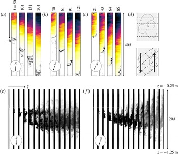
(a,b,c) The evolution of the reduced gravity $g^{\prime }(x,z,t)$ during typical experiments using our image analysis method for tilt angles of 0°, 15° and 30°, corresponding to $B_{s}=10\times 10^{-7}~\text{m}^{4}~\text{s}^{-3}$ , $B_{s}=20\times 10^{-7}~\text{m}^{4}~\text{s}^{-3}$ and $B_{s}=20\times 10^{-7}~\text{m}^{4}~\text{s}^{-3}$ respectively. The sequence of images shown for each tilt angle corresponds to times $\tilde{t}=0.25\tilde{t}_{f}$ , $0.5\tilde{t}_{f}$ , $0.75\tilde{t}_{f}$ and $\tilde{t}_{f}$ . The colours of each sequence of images are adjusted so that the maximum reduced gravity observed in an experiment corresponds to black. In each image, we also show a black contour line where $g^{\prime }=7.5\times 10^{-4}~\text{m}~\text{s}^{-2}$ , indicating the location of the front as it propagates down the length of the tank. (d) A cartoon of the flow pattern that develops within the mixed fluid when ${\it\theta}=0^{\circ }$ and ${\it\theta}>0^{\circ }$ . Dashed black lines indicate reduced gravity contours and solid black arrows indicate the counterflow that develops when ${\it\theta}>0^{\circ }$ ; here, the upward-facing boundary is on the left and the downward-facing boundary is on the right. (e,f) Snapshots of the evolution of the buoyancy-induced turbulent flow for ${\it\theta}=0^{\circ }$ and ${\it\theta}=15^{\circ }$ respectively for our dye experiments. These experiments are conducted with clear dense source fluid, and in order to show qualitatively the structure of the mixing region, a small volume of very dark dye is released with a long thin metal tube and a syringe at $\tilde{t}=\tilde{t}_{f}/2$ into the clear mixed region of fluid at $x=-d/2,z=-10d$ .

2.4. Experimental observations

During an experiment, the dense source fluid mixes into the fresh clear water, and a region of mixed fluid slowly propagates towards the bottom of the tank. In figure 2(a–c), we show snapshots of the evolution of $g^{\prime }$ based on our image analysis procedure at times $\tilde{t}=0.25\tilde{t}_{f}$ , $0.5\tilde{t}_{f}$ , $0.75\tilde{t}_{f}$ and $\tilde{t}_{f}$ for ${\it\theta}=0^{\circ }$ , 15° and 30° respectively, for typical experiments. Based on this, it is immediately apparent that $\tilde{t}_{f}$ decreases with ${\it\theta}$ , already suggesting that the efficacy of mixing along the tank may be enhanced when the tank is tilted. Furthermore, it is clear that a cross-tank gradient of $g^{\prime }$ forms when ${\it\theta}>0^{\circ }$ . It should be noted that, as shown in figure 2(c), the mixed fluid is able to mix turbulently across the entire width of the tank for the majority of the mixed region even at ${\it\theta}=30^{\circ }$ .

In order to probe the effect that the cross-tank component of gravity has on the turbulent eddies, we estimate the overall cross-tank gradient of reduced gravity across the width of the tank as

where ${\hat{g}}^{\prime }=g^{\prime }-\overline{g^{\prime }}$ is the fluctuation of reduced gravity from the cross-tank averaged value and $x^{\ast }=x^{\ast }(z,t)$ is the coordinate along the width of the tank where the magnitudes of the two integrals in the round brackets in (2.7) are both equal and maximised. Specifically, we may define this coordinate as

where in an ensemble average, $x^{\ast }$ is typically equal to 0. Physically, $x^{\ast }$ indicates the location across the width of the tank that divides an excess of buoyancy from a deficiency of buoyancy of equal magnitude – a measure of the ‘centre’ of the profile. We note that, in general, there may exist cross-sections in the tank where there does not exist a unique $x^{\ast }$ , but the nature of experimental measurements makes this possibility statistically very unlikely. Defined in this way, if $G_{x}>0$ , then fluid close to the downward-facing boundary at $x=d/2$ is generally denser, and if $G_{x}<0$ , then fluid close to the upward-facing boundary at $x=-d/2$ is generally denser.

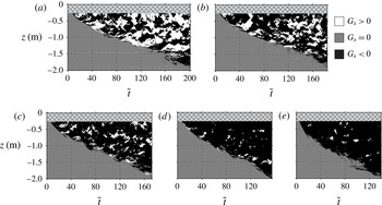
For experiments with ${\it\theta}=0^{\circ }$ , there is an irregular and time-dependent variation in the reduced gravity across the width of the tank, and this variation is associated with the turbulent eddies. While, in general, instantaneous cross-tank gradients of reduced gravity of either sign may form, in an ensemble average, we expect this gradient to be equal to zero. Figure 3(a) shows a spatiotemporal diagram of the evolution of the gradient in reduced gravity across the width of the tank $G_{x}$ as defined in (2.7) for a typical experiment with ${\it\theta}=0^{\circ }$ , indicating that turbulent mixing events in the tank characterised by both $G_{x}>0$ and $G_{x}<0$ are approximately equally likely. This in turn leads to a natural hypothesis that there is no preference in the sense of the vorticity of the rapidly evolving eddies.

Figure 3.

Spatiotemporal diagrams depicting the evolution of the sign of the cross-tank gradient of reduced gravity $G_{x}$ through non-dimensional time $\tilde{t}$ for typical experiments with (a) ${\it\theta}=0^{\circ }$ , (b) ${\it\theta}=2.5^{\circ }$ , (c) ${\it\theta}=5^{\circ }$ , (d) ${\it\theta}=7.5^{\circ }$ and (e) ${\it\theta}=10^{\circ }$ . Each vertical column of pixels represents the sign of $G_{x}$ throughout the tank at a particular time step. Black corresponds to $G_{x}<0$ , grey corresponds to $G_{x}=0$ and white corresponds to $G_{x}>0$ . The light grey cross-hatched band at the top of each diagram corresponds to the region of length $5d$ at the top of the tank where the dynamics of the source strongly affects the structure of the cross-tank gradient. We note that this figure also graphically shows the propagation of the front of the mixed region of fluid down the length of the tank throughout an experiment.

However, when ${\it\theta}>0^{\circ }$ , the effect of a cross-tank component of gravity is clearly evident in the snapshots of figure 2(b–c). This body force acts to segregate the heavy and light fluids such that the frequency of occurrence of regions with statically stable density gradient $(\partial g^{\prime }/\partial x)<0$ is higher than that of regions with statically unstable density gradient, suggesting that the ensemble average of $(\partial g^{\prime }/\partial x)<0$ . Figure 3(b–e) shows the evolution of $G_{x}$ for typical experiments with ${\it\theta}=2.5^{\circ }$ , ${\it\theta}=5^{\circ }$ , ${\it\theta}=7.5^{\circ }$ and ${\it\theta}=10^{\circ }$ respectively, and demonstrates that as ${\it\theta}$ increases, turbulent mixing events where $G_{x}>0$ (shown in white) occur less frequently in the mixing region. When ${\it\theta}=10^{\circ }$ , it is observed that the overall cross-tank gradient is almost always negative ( $G_{x}<0$ , shown in black), and that the fluid is stably stratified across the width of the tank throughout the majority of an experiment. In all the cases considered in this paper, however, it is observed that the turbulent eddies typically grow to a size comparable to the width of the tank within a distance $O(5d)$ from the top of the tank (as described in VS12 for the case of ${\it\theta}=0^{\circ }$ ), and, therefore, there may be differences between experiments and our model developed in § 3 within this region. As is apparent in figure 3, the period over which the eddies initially grow to the full width of the tank is relatively short, and does not depend strongly on the tilt angle.

When ${\it\theta}>0^{\circ }$ , fluid within the mixed region close to the upward-facing boundary of the tank at $x=-d/2$ tends to have a larger reduced gravity than the cross-tank averaged reduced gravity; similarly, fluid close to the downward-facing boundary of the tank at $x=d/2$ tends to have a smaller reduced gravity. In other words, in an ensemble average, $g^{\prime }(x=-d/2,z,t)>\overline{g^{\prime }}(z,t)>g^{\prime }(x=d/2,z,t)$ within the mixed region of fluid. This cross-tank profile of $g^{\prime }(x,z,t)$ , coupled with the statically unstable distribution of fluid along the length of the tank, $(\partial \overline{g^{\prime }}/\partial z)>0$ , therefore leads to the natural hypothesis that, on average, a velocity profile is formed along the length of the mixed region where heavier fluid near $x=-d/2$ flows downwards and lighter fluid near $x=d/2$ flows upwards. This hypothesis is shown as a cartoon in figure 2(d), along with qualitative differences in the reduced gravity contours when the tank is tilted, although it is important to appreciate that there is always at least some source fluid mixed across the entire width of the tank.

To examine further this hypothesised counterflow structure and the effect it may have on the overall evolution of the flow qualitatively, we conduct an experiment where we focus on a specific area within the mixed region of the buoyancy-driven flow. We inject clear dense source fluid at the top of the tank and release a small volume of very concentrated dark dye at a point into this clear mixed region behind the front. We release this small volume of dye at approximately half of the time that it takes for the front of the mixing region to reach the bottom of the tank, $\tilde{t}=\tilde{t}_{f}/2$ , for each tilt angle. The small volume of dye is released at $x=-d/2,z=-10d$ with a thin metal tube and a syringe, and the density of the small volume of dye is approximately matched to the density at the release point by initially drawing in a small amount of the fluid in the mixed region into the syringe. The small volume of dye is released relatively slowly from the thin metal tube (over approximately 2 s) to minimise any jet-like effects. We conduct this experiment at ${\it\theta}=0^{\circ }$ and ${\it\theta}=15^{\circ }$ , to compare the purely vertical mixing with that which arises when there is significant inclination to the vertical. The experiments are conducted with the same buoyancy flux of $B_{s}=10\times 10^{-7}~\text{m}^{4}~\text{s}^{-3}$ . For this experiment at ${\it\theta}=15^{\circ }$ , we choose to use a buoyancy flux of $B_{s}=10\times 10^{-7}~\text{m}^{4}~\text{s}^{-3}$ instead of $B_{s}=20\times 10^{-7}~\text{m}^{4}~\text{s}^{-3}$ , as discussed in § 2.3, in order to compare the experiments at the two different tilt angles directly. In addition, we are not concerned with low-Reynolds-number effects near the front for these experiments, because we focus on a section within the mixed region of fluid where we inject the dye.

In figure 2(e–f), we show the line-of-sight light intensities in the region $-25d\leqslant z\leqslant -5d$ of sequences of images obtained every 2 s for ${\it\theta}=0^{\circ }$ and ${\it\theta}=15^{\circ }$ respectively. When the tank is vertical, it is apparent that turbulent eddies of size $O(d)$ disperse the small volume of dye rapidly and homogeneously into the mixing region. These observations are consistent with the particle image velocimetry (PIV) measurements of turbulent Rayleigh–Taylor experiments described in Dalziel et al. (Reference Dalziel, Patterson, Caulfield and Coomaraswamy2008), which suggested that vortical structures in flows of similar Reynolds numbers had an aspect ratio of ${\approx}1$ with a size governed by the width of the tank. As predicted, there does not appear to be a preference in the orientation of the overturning eddies, and there is little variation of dye concentration in the cross-tank direction. However, at ${\it\theta}=15^{\circ }$ , it is apparent that the cross-tank component of gravity has qualitatively changed the flow. After the dye is introduced and mixed across the width of the tank, a portion of the dye is rapidly advected down along the upward-facing boundary of the tank at $x=-d/2$ , and, similarly, a portion of the dye is rapidly advected up along the downward-facing boundary of the tank at $x=d/2$ . These observations support our hypothesis that a counterflowing velocity field develops in an inclined tank due to the cross-tank gradient in reduced gravity. It is also apparent that the flow remains turbulent when the tank is tilted. The turbulent eddies still grow and are confined in the cross-tank direction to the width $d$ of the tank, which suggests that the evolution of $g^{\prime }$ may be described as a turbulent diffusive process when ${\it\theta}>0^{\circ }$ in a way similar to the turbulent diffusive behaviour observed when ${\it\theta}=0^{\circ }$ . The observation of the shear flow superposed on the turbulently mixing flow may lead to an enhanced flux of buoyancy along the tank, and we now explore this by developing our model and presenting a quantitative analysis of the experimental measurements.

3.1. Evolution equation for reduced gravity

We consider the buoyancy-induced turbulent mixing in a long narrow tank of dimensions $d\times d\times H$ tilted at an angle ${\it\theta}$ from the vertical, where a constant buoyancy flux $B_{s}$ of dense source fluid is introduced at the top of the tank. The dense source fluid mixes into the fresh clear water, and, in general, we may write an evolution equation for $g^{\prime }$ as

where $\boldsymbol{u}=u\boldsymbol{e}_{x}+w\boldsymbol{e}_{z}$ is the velocity field that is associated with the turbulent mixing. We have ignored fluxes due to molecular diffusion, which we would expect to be negligible compared with the effects of turbulence. Due to the turbulent structure of the flow, we choose to decompose $\boldsymbol{u}$ and $g^{\prime }$ as

where $\langle \boldsymbol{u}\rangle _{e}$ and $\langle g^{\prime }\rangle _{e}$ denote the ensemble averaged velocity and reduced gravity respectively, and $\boldsymbol{u}_{eddy}$ and $g_{eddy}^{\prime }$ denote the instantaneous fluctuations in velocity and reduced gravity which are associated with the turbulent eddies respectively. We will use $\langle -\rangle _{e}$ to denote an ensemble average, and we note that this averaging process is essentially equivalent to averaging over several time scales of the overturning turbulent eddies to remove the effect of turbulent fluctuations, assuming that the time scale for the evolution of the underlying flow is longer than the overturning time of an eddy. We may further decompose the ensemble averaged quantities as

where $\langle \overline{\boldsymbol{u}}\rangle _{e}$ and $\langle \overline{g^{\prime }}\rangle _{e}$ denote the cross-tank averaged components of the ensemble averaged velocity and reduced gravity respectively, and $\langle \hat{\boldsymbol{u}}\rangle _{e}$ and $\langle {\hat{g}}^{\prime }\rangle _{e}$ denote the fluctuations from the cross-tank averages of the ensemble averaged velocity and reduced gravity respectively. We note that because we do not impose any forced advection in the tank $\langle \overline{\boldsymbol{u}}\rangle _{e}=\mathbf{0}$ , and, by definition, $\langle \boldsymbol{u}_{eddy}\rangle _{e}=\mathbf{0}$ and $\langle g_{eddy}^{\prime }\rangle _{e}=0$ . Importantly, we note that the ensemble average of the fluctuation of the along-tank velocity from its cross-tank average $\langle {\hat{w}}\rangle _{e}\neq 0$ , while $\langle \hat{u} \rangle _{e}=0$ , due to the observed counterflow structure in the tank. The ensemble average of the general evolution equation (3.1) is thus

Written in this way, the ensemble average reveals the extra nonlinear contribution of the turbulent motions, i.e. $\langle \boldsymbol{u}_{eddy}\boldsymbol{\cdot }\boldsymbol{{\rm\nabla}}g_{eddy}^{\prime }\rangle _{e}$ . This term describes the advection of reduced gravity due to the motion of the buoyancy-induced turbulent eddies, and we model it as an eddy diffusion term according to Fick’s law, so that (3.4) becomes

where $\unicode[STIX]{x1D646}$ is the turbulent diffusivity tensor, and ${\it\kappa}_{T,x}$ and ${\it\kappa}_{0}$ are the turbulent diffusion coefficients characterising the mixing associated with the turbulent eddies across the width of the tank and along the length of the tank respectively.

Based on this eddy diffusion model, the ensemble averaged evolution equation (3.5) may be cross-tank averaged across the width of the tank to obtain

upon applying the no-flux boundary conditions at $x=\pm d/2$ . Here, $T_{T}$ , $T_{A}$ and $T_{D}$ are the time-dependent, advection and eddy diffusion terms respectively.

The nonlinear advection term $T_{A}$ on the left-hand side of (3.6) is a direct consequence of the counterflow structure. When ${\it\theta}=0^{\circ }$ , i.e. the case studied by VS12 when there is no ensemble averaged counterflow, this term is equal to zero, and so the evolution of the turbulent eddies is only governed by the turbulent diffusion coefficient ${\it\kappa}_{0}$ . Our experimental observations in § 2 suggest that the counterflow acts to enhance the efficacy of mixing along the tank, and so we develop a model for this nonlinear advection term $T_{A}$ .

By taking the difference between the ensemble averaged evolution equation (3.5) and its cross-tank averaged counterpart (3.6), we obtain an evolution equation for the fluctuations of reduced gravity from its cross-tank averaged value, i.e.

To simplify this evolution equation, we introduce the ansatz that the leading-order balance of (3.7) is

showing that there is a balance between the cross-tank turbulent flux of $\langle {\hat{g}}^{\prime }\rangle _{e}$ and the along-tank advection of $\langle \overline{g^{\prime }}\rangle _{e}$ , which we note is analogous with the analysis of Taylor dispersion (Taylor Reference Taylor1953). This turbulent flux of $\langle {\hat{g}}^{\prime }\rangle _{e}$ across the width of the tank is defined as

As a closure to determine the counterflow velocity $\langle {\hat{w}}\rangle _{e}$ , we consider a momentum balance in $z$ from the Navier–Stokes equations in the tilted coordinate system defined in figure 1, such that

where, again, we neglect molecular diffusion. By substituting (3.2) and (3.3) and taking an ensemble average, we deduce that

where $\partial \langle \hat{p}\rangle _{e}/\partial z$ is the non-hydrostatic component of the pressure gradient. To obtain (3.11), we have subtracted out the hydrostatic contribution of the pressure gradient. Analogously to (3.5), we model the transport of momentum due to the turbulent motions, i.e.  $\langle \boldsymbol{u}_{eddy}\boldsymbol{\cdot }\boldsymbol{{\rm\nabla}}w_{eddy}\rangle _{e}$ , as an eddy diffusion term and assume (as a related ansatz to (3.8)) that the leading-order balance of (3.11) is

where $\mathit{Sc}_{T}$ is the turbulent Schmidt number, i.e. the ratio of the turbulent diffusivities of momentum and density. We note that assumptions (3.8) and (3.12) can indeed be shown to be the leading-order balances in time based on the following discussion and the scalings presented in § 4, at least in the limit of sufficiently small tilt angles ${\it\theta}$ .

Specifically, it is important to appreciate that the neglect of the non-hydrostatic pressure gradient (the first term on the right-hand side of (3.11)) is only formally valid for small angles. Particularly at larger angles, it is reasonable to assume that there is a ‘baroclinic pressure gradient’, as discussed, for example, for horizontally propagating gravity currents in the presence of turbulence by Linden & Simpson (Reference Linden and Simpson1986). This pressure gradient is associated with an along-tank force due to along-tank variations in the cross-tank fluctuating buoyancy. Straightforward scaling arguments suggest that this term should scale with the cross-tank component of the gravity, and so

where $h$ is the characteristic along-tank height of the mixed region. Therefore, we expect this term to be negligible by comparison with the second term on the right-hand side of (3.11) used in the assumed leading-order balance (3.12) when

Clearly, our modelling assumption ignoring this pressure gradient term will break down when the tank is horizontal, and ${\it\theta}\rightarrow 90^{\circ }$ . However, even for angles as high as 45°, the condition (3.14) is being approached when the mixed region has propagated $5-10d$ down the tank. As already noted, and discussed in more detail in VS12, the specific flow structure at the source affects the flow in a region of $5d$ at the top of the tank. Therefore, we believe that the leading-order balance (3.12) is appropriate to describe the flow evolution in the tank that we are considering, although it is always important to appreciate that for larger angles, the increasing influence of this pressure gradient term may lead to a discrepancy between our model and experiments.

For the following analysis, we will make the further simplifying assumption that both $\mathit{Sc}_{T}$ and ${\it\kappa}_{T,x}$ are constant in $x$ . In this way, we will conduct a leading-order analysis of the cross-tank mixing. Substituting the momentum balance (3.12) into the leading-order evolution equation for $\langle {\hat{g}}^{\prime }\rangle _{e}$ (3.8), we obtain the governing boundary value equation for $\langle {\hat{w}}\rangle _{e}$ ,

where we have non-dimensionalised $x$ as $\tilde{x}=x/d$ and where the eigenvalues of this boundary value problem are

To solve (3.15), we impose the no-slip condition at the boundaries,

and the no-flux condition at the boundaries,

where we have used (3.12) in order to write this boundary condition in terms of $\langle {\hat{w}}\rangle _{e}$ . With the boundary conditions (3.17) and (3.18), it is then possible to decouple the even and odd components of the solution to (3.15). Specifically, we deduce that there is an independent eigenvalue relation for solutions that are even about $\tilde{x}=0$ and an independent eigenvalue relation for solutions that are odd about $\tilde{x}=0$ , so that

Based on our observation of the presence of a turbulent counterflow structure across the width of the tank, we predict that the solution $\langle {\hat{w}}\rangle _{e}$ is odd about $\tilde{x}=0$ , and we expect $\langle {\hat{w}}\rangle _{e}$ to have a mode-2 shape, i.e. where dense fluid flows downwards in $\tilde{x}<0$ and lighter fluid flows upwards in $\tilde{x}>0$ . Therefore, we choose the first non-trivial root of the odd eigenvalue relation, given by ${\it\beta}_{\ast }=4.73$ . Furthermore, equations (3.15), (3.17) and (3.18) define a non-self-adjoint boundary value problem, and the eigenfunctions associated with distinct eigenvalues are not orthogonal. Therefore, in this leading-order model, we neglect the potential contributions of the higher modes corresponding to larger eigenvalues. Then, the solution to (3.15) is given by

where ${\hat{W}}={\hat{W}}(z,t)$ is the amplitude of the velocity fluctuations. Consistently with (3.8) and (3.12), we employ the further ansatz that the amplitude of the velocity fluctuations is proportional to the square root of the reduced gravity gradient along the tank, so that

where ${\it\gamma}$ is an $O(1)$ constant which may be determined through experiments. We note that in the case of ${\it\theta}=0^{\circ }$ , we expect ${\it\gamma}=0$ , because there is no counterflow. This form of $\langle {\hat{w}}\rangle _{e}$ is consistent with our observations of a turbulent counterflow structure which is odd about $\tilde{x}=0$ . In this way, we may also estimate the mean velocity $\langle {\hat{w}}\rangle _{e,m}$ of the counterflow by integrating (3.20) from $\tilde{x}=0$ to $\tilde{x}=1/2$ (or, equivalently, from $\tilde{x}=-1/2$ to $\tilde{x}=0$ , which would yield a mean velocity with an opposite sign). Therefore, we deduce that the mean counterflow velocity is given by

By substituting (3.20) into (3.12), we deduce that the form of $\langle {\hat{g}}^{\prime }\rangle _{e}$ given by our leading-order model is

where, in this context, ${\it\gamma}$ captures the asymmetry of the reduced gravity profile introduced by the cross-tank component of gravity and where ${\hat{G}}={\hat{G}}(z,t)$ is the corresponding amplitude, which is given by

This form of $\langle {\hat{g}}^{\prime }\rangle _{e}$ decreases monotonically with $\tilde{x}$ . Based on the first root ${\it\beta}={\it\beta}_{\ast }$ of the odd eigenvalue relation defined in (3.19b ), we may also deduce from the definition of the eigenvalues in (3.16) that the turbulent diffusion coefficient characterising the mixing across the width of the tank is

Based on the forms of $\langle {\hat{w}}\rangle _{e}$ and $\langle {\hat{g}}^{\prime }\rangle _{e}$ derived here ((3.20) and (3.23) respectively), we may now determine the advection term $T_{A}$ of (3.6). We deduce that

since

for ${\it\beta}_{\ast }=4.73$ , the first non-trivial root of (3.19b ). The term $T_{A}$ is negative, as expected, and shows that the balance of the along-tank shear and the cross-tank mixing acts to enhance the net transport along the tank. Furthermore, the dependence on $\partial \langle \overline{g^{\prime }}\rangle _{e}/\partial z$ is consistent with the diffusive term $T_{D}$ derived with Prandtl’s mixing length theory used in VS12 for a purely vertical tank, which assumed that

where $l_{0}$ and $w_{0}$ are the mixing length and the buoyancy-driven speed due to the turbulent eddies respectively. This form of ${\it\kappa}_{0}$ is also consistent with the models presented by Holmes et al. (Reference Holmes, Karr and Baird1991), Baird et al. (Reference Baird, Aravamudan, Rao, Chadam and Peirce1992) and Zukoski (Reference Zukoski1995). However, in a tilted tube, we expect the contribution from the turbulent diffusion along the tank to be reduced by a factor $\sqrt{\cos {\it\theta}}$ since the component of gravity along the tank is reduced by the factor $\cos {\it\theta}$ , thereby reducing the buoyancy-driven speed due to the turbulent eddies by an amount $\sqrt{\cos {\it\theta}}$ . Based on (3.26), this analysis shows that the ensemble averaged advection term $T_{A}$ in (3.6) acts to modify the effective turbulent diffusion due to the eddies directly. Therefore, we conclude that the governing evolution equation for $\langle \overline{g^{\prime }}\rangle _{e}$ can be written as

where

using (3.26) and (3.27) with ${\it\lambda}_{0}$ the coefficient for a vertical tube (VS12), which was observed to be ${\it\lambda}_{0}\simeq 1$ . This prediction for ${\it\lambda}$ as a function of ${\it\theta}$ represents the combination of the along-tank eddy mixing and the cross-tank eddy mixing associated with the shear. It may be shown that this prediction is self-consistent with the three key assumptions (3.8), (3.12) and (3.21). This analysis shows that the contribution of the counterflow $T_{A}$ can be summed directly with the divergence of the diffusive flux due to the turbulent eddies $T_{D}$ as both terms have the same dependence on $\partial \langle \overline{g^{\prime }}\rangle _{e}/\partial z$ . This indicates that the same equation governs the evolution of $\langle \overline{g^{\prime }}\rangle _{e}$ when the tank is tilted as when the tank is vertical, as originally discussed by VS12, except for the change in the empirical coefficient from ${\it\lambda}_{0}$ to ${\it\lambda}$ .

We expect the empirical coefficient ${\it\lambda}={\it\lambda}_{0}\simeq 1$ only when the tank is vertical, i.e. when there is no ensemble averaged counterflow described by the term $T_{A}$ in (3.6). Based on our analysis, we expect the effective along-tank turbulent diffusion coefficient, ${\it\kappa}_{T,z}$ , to be

Again, consistently with Prandtl’s mixing length theory, $l_{T,z}$ and $w_{T}$ are the effective mixing length and buoyancy-induced speed along the tank due to both the turbulent eddies and the counterflow. This then shows that the turbulent flux of $\langle \overline{g^{\prime }}\rangle _{e}$ along the tank is equal to

Posed in this way, the assumed constant coefficient ${\it\lambda}$ that relates the effective mixing length to the width of the tank characterises the efficacy of mixing down the length of the tank, due to both the turbulent eddies and the counterflow. We now explore whether this model is consistent with the experimental data from the experiments we described in § 2.

4.1. Scaling properties and transition to the self-similar regime

When ${\it\theta}=0^{\circ }$ , VS12 showed that the height of the mixed region of fluid grows like

and that the reduced gravity at the top of the tank grows like

which is based on both dimensional analysis of the parameters controlling the experiment and the conservation of mass constraint (2.5) which states that $\overline{g^{\prime }}_{T}(0)h_{T}=B_{s}d^{-2}t$ . Since the flux is constant, the source location is fixed, and we only consider the flow during the ‘initial mixing phase’ of VS12, so that the total amount of buoyancy is conserved within the tank, we expect the distribution of reduced gravity to converge towards a self-similar solution, specifically starting at $\tilde{t}=0$ .

These scalings (4.1) and (4.2) naturally lead to a self-similar relation,

where the shape function $f$ is the reduced gravity non-dimensionalised by this proposed scaling for the reduced gravity at the top of the tank, and ${\it\eta}$ is the natural similarity variable. When ${\it\theta}>0^{\circ }$ , the same parameters ( $B_{s}$ and $d$ ) control the experiment, and so we expect these scalings to be still valid. As discussed in more detail in Lin (Reference Lin2014), this can be shown to be the case at least for sufficiently small angles, except for an initial ‘flow establishment’ regime which does not follow these scalings due to the presence of a cross-tank component of gravity.

In each experiment, there is an initial period when the flow adjusts to the self-similar spreading before reaching the bottom of the tank. During this ‘flow establishment’ regime, there appears to be a finite value of the buoyancy at the front of the advancing current of dense fluid (as measured by the cross-tank average of reduced gravity), which is in contrast to the self-similar solution, where the buoyancy drops off to zero at the front. The data suggest that the distance the current travels before it appears to converge to the self-similar asymptotic solution increases as the angle of tilt increases. These observations may be related to a transition from a gravity current type of flow at early times, before the flow has mixed fully across the tank, to the present model once the flow has become mixed. That the present mixing regime eventually dominates the gravity driven flow is due to the fact that as the flow develops, a greater depth of the flow is mixed in the cross-tank direction at positions nearer the source. As a result, the flow initially adjusts to the self-similar mixing regime in regions near the source, and then this mixing zone advances down the tank. Since the self-similar mixing involves a transport of buoyancy along the tank at a slower speed than the speed of the gravity current head, the gravity current becomes deprived of a continuing source of buoyancy, and hence actually reduces in extent as it mixes, leading to the adjustment of the whole current towards the self-similar mixing regime. However, the current takes a greater distance to asymptote on a slope, because the cross-tank mixing is less effective on a slope. This is evidenced by the cross-tank gradient in reduced gravity and the along-tank shear flow which leads to the gravity current being supplied with buoyancy and hence reaching a greater distance down the tank prior to full adjustment to the self-similar solutions of interest herein.

4.2. Turbulent mixing along the tank

When the tank is tilted at a non-trivial angle from the vertical, the experimental data are observed to follow the scaling laws (4.1) and (4.2) after a transient ‘flow establishment’ regime, and, in this paper, we will focus on the application of our model solely to the self-similar regime of our experiments. Therefore, following VS12, we non-dimensionalise the nonlinear evolution equation (3.29) for $\langle \overline{g^{\prime }}\rangle _{e}$ with the non-dimensional reduced gravity $f$ and similarity variable ${\it\eta}$ defined in (4.3), so that

As discussed above, we predict that ${\it\lambda}={\it\lambda}({\it\theta})$ , and for a particular value of ${\it\lambda}$ , we impose two conditions in order to solve (4.4) numerically. The first condition states that the turbulent flux of $\langle \overline{g^{\prime }}\rangle _{e}$ (given by (3.32)) at the top of the tank is equal to $B_{s}d^{-2}$ , which in non-dimensional form corresponds to

Furthermore, the second condition (2.5) states that the total buoyancy in the tank rises linearly in time as $B_{s}t$ , which is equivalent to

where ${\it\eta}_{H}=-H/h_{T}$ is the bottom of the tank in self-similar space. We solve (4.4) numerically with a shooting multistep method in MATLAB. First, we guess a value of ${\it\lambda}$ which we expect to be of $O(1)$ , which sets the flux condition (4.5). Then, we search for the boundary value $f(0)$ that minimises the error in satisfying the conservation of buoyancy constraint (4.6), and this error is within $\pm 5\times 10^{-4}$ . We then determine the squared error between this numerical solution and the experimentally determined profile, and then repeatedly update our choice of ${\it\lambda}$ until the value of ${\it\lambda}$ minimising this squared error is found. The experimental profile for each tilt angle is determined by time averaging over the extent of the self-similar regime and ensemble averaging over three separate trials. Furthermore, in this fitting procedure, the data corresponding to the region of length $5d$ at the top of the tank are ignored, because we expect deviations from our model to occur there. Based on this procedure of matching our theoretical prediction with our experimental data, we can determine the optimal ${\it\lambda}$ that best fits the solution of (4.4) with the experimental profiles for each tilt angle tested.

Figure 4.

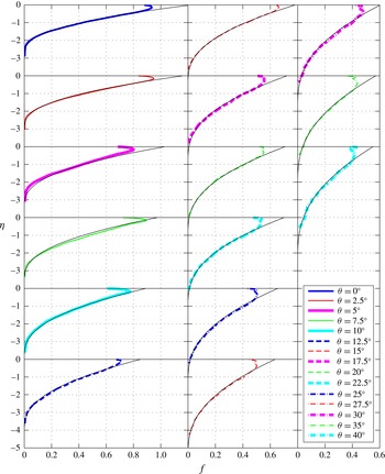
Profiles of non-dimensional cross-tank averaged reduced gravity for the experiments time averaged over the self-similar regime and ensemble averaged over three trials with ${\it\theta}=0^{\circ }$ , 2.5°, 5°, 7.5°, 10°, 12.5°, 15°, 17.5°, 20°, 22.5°, 25°, 27.5°, 30°, 35° and 40°. Angles increase down the columns, and then from left to right. These experimental profiles are plotted with the numerical solutions $f$ of (4.4) (shown by black lines) which correspond to the value of ${\it\lambda}$ that minimises squared error. 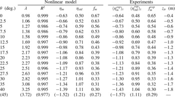These values for ${\it\lambda}={\it\lambda}({\it\theta})$ are tabulated in table 1.

In figure 4, the numerical solutions $f$ to (4.4) are plotted with solid black lines. For all of the angles tested, the solutions $f$ smoothly converge to zero at a value ${\it\eta}={\it\eta}_{f}$ , representing the front of the mixed region of fluid. This finite front coordinate ${\it\eta}_{f}$ decreases with increasing ${\it\theta}$ , from ${\it\eta}_{f}\approx -3.1$ when ${\it\theta}=0^{\circ }$ (shown in the top panel of the leftmost column) to ${\it\eta}_{f}\approx -6.7$ when ${\it\theta}=40^{\circ }$ (shown in the bottom panel of the rightmost column), indicating that the propagation of the front of the mixed region of fluid is significantly faster when the tank is tilted. We also plot the corresponding experimental profiles $f^{exp}$ (the superscript $\mathit{exp}$ referring to an experimental quantity), which are given by

where $\langle -\rangle _{t}$ denotes a time average over the self-similar regime, and, as noted before, $\langle -\rangle _{e}$ denotes an ensemble average over three trials. The flow transitions to this self-similar regime from the ‘flow establishment’ regime, as discussed previously, when the front of the mixed region passes $z=z_{tr}$ , as tabulated in table 1. This length increases monotonically with tilt angle ${\it\theta}$ , and for ${\it\theta}=45^{\circ }$ we do not observe this self-similar transition before the front of the mixed region reaches the bottom of the tank at $z=-2~\text{m}$ . Here, all of the data, including the data within the length $5d$ at the top of the tank, are plotted. Our model agrees well with our experimental data, except near the source and, to a lesser extent, close to the front ${\it\eta}_{f}$ . Typically, ${\it\eta}_{f}<{\it\eta}_{f}^{exp}$ , and this discrepancy increases with increasing ${\it\theta}$ ; our experimental data show that ${\it\eta}_{f}^{exp}\approx -2.9$ when ${\it\theta}=0^{\circ }$ and ${\it\eta}_{f}^{exp}\approx -4.6$ when ${\it\theta}=40^{\circ }$ . As noted before, the majority of the mixed region of fluid is able to mix turbulently across the width of the tank. However, at the front of the mixed region, a ‘nose’ that has a small length of $O(d)$ is observed to be unable to mix across the entire width, even in the self-similar regime. Furthermore, $f({\it\eta})\ll 1$ as ${\it\eta}\rightarrow {\it\eta}_{f}$ , and such small values are difficult to detect experimentally. When ${\it\theta}>0^{\circ }$ , turbulent eddies which are supplied from the counterflow of the mixed region break up rapidly along the upward-facing boundary in the ‘nose’. Due to the asymmetry introduced by the cross-tank component of gravity, this ‘nose’ is unable to mix across the width fully and become fully diluted by the available fresh fluid. Therefore, as ${\it\theta}$ increases, the convergence of $f^{exp}\rightarrow 0$ as ${\it\eta}^{exp}\rightarrow {\it\eta}_{f}^{exp}$ becomes less smooth. However, it is clear from figure 4 that this region is very dilute when compared with the rest of the mixed region of fluid.

Table 1.

The first moment ${\it\eta}_{m}$ , standard deviation ${\it\eta}_{std}$ and non-dimensional reduced gravity corresponding to the first moment $f_{m}=f({\it\eta}_{m})$ determined from our model with the value of ${\it\lambda}$ that minimises squared error for each tilt angle tested, along with the values of $R^{2}$ indicating the good quality of fit between our numerical solutions $f$ and experimental profiles $f^{exp}$ . Also shown are the values $\langle {\it\eta}_{m}^{exp}\rangle _{t}$ and $\langle {\it\eta}_{std}^{exp}\rangle _{t}$ time averaged over the self-similar regime of each experiment along with $f_{m}^{exp}=f^{exp}(\langle {\it\eta}_{m}^{exp}\rangle _{t})$ . In each experiment, the flow transitions to the self-similar regime when the front of the mixed region passes $z=z_{tr}$ . The values corresponding to ${\it\theta}=45^{\circ }$ are shown in parentheses and are only estimates: the flow was not observed to transition to a self-similar regime within our experimental tank for this tilt angle.

Figure 5.

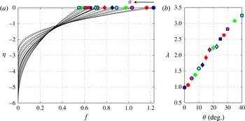
(a) All of the numerical solutions $f$ of (4.4) plotted against the self-similar coordinate ${\it\eta}$ corresponding to the values of ${\it\lambda}$ that minimise the squared error between the numerical solutions and the experimental profiles. The symbols plotted at ${\it\eta}=0$ correspond to the symbols shown in (b), which shows the best-fit values of ${\it\lambda}({\it\theta})$ that correspond to the tilt angles tested, as tabulated in table 1.

Aside from the region close to the source and the small ‘nose’ at the front introduced by the cross-tank component of gravity, the shapes of the profiles predicted by the nonlinear turbulent diffusion equation (4.4) agree well with experiments. From this model, we may also calculate the predicted values of the first moment of $f$ , i.e. the centre-of-mass, defined as

and the standard deviation ${\it\eta}_{std}$ about the first moment of $f$ ,

along with the non-dimensional reduced gravity corresponding to the first moment,

Due to the shape of the solutions, the first moment of $f$ is observed to decrease with increasing ${\it\theta}$ while the standard deviation increases. These quantities are tabulated in table 1, along with the values of $R^{2}$ indicating the good quality of fit between our numerical solutions $f$ and experimental profiles $f^{exp}$ (the region of length $5d$ at the top of the tank is ignored) and the experimental values for $\langle {\it\eta}_{m}^{exp}\rangle _{t}$ and $\langle {\it\eta}_{std}^{exp}\rangle _{t}$ . The high $R^{2}$ values, which are consistent with the errors of our image analysis method, and the close agreement between these predictions and the experimental quantities time averaged over the self-similar regime further reinforce our confidence in our modelling approach. Interestingly, it is clear from figure 4 that there is no need to shift the experimental profiles $f^{exp}$ to a virtual origin (in space or time) in order to match the numerical solutions $f$ , even though there is an initial transient ‘flow establishment’ regime that probably follows a different scaling in time. In the case of an unbounded plume issued from a pure point source of buoyancy, Morton et al. (Reference Morton, Taylor and Turner1956) discussed the need for a virtual origin (in space) in order to take into account details of the source, i.e. a non-ideal source of finite size, and various models have been developed to describe this fitting (see, e.g., Caulfield & Woods Reference Caulfield and Woods1995; Hunt & Kaye Reference Hunt and Kaye2001). In the flow that we consider, however, while the flow travels a distance from the source in order to transition from a gravity-current-like flow to a self-similar regime, this final self-similar form of the flow is not associated with local conditions of the source. In fact, in the self-similar regime, fine details of the source are unlikely to affect the overall flow; rather, the flow is controlled by the total (integral) buoyancy that has been added to the mixed fluid, which linearly increases from zero with time. Indeed, mathematically a virtual origin offset in time would lead to the total buoyancy in the self-similar solution not matching the actual total buoyancy within the tank.

In figure 5(a), we plot all of the profiles of $f$ predicted by our model corresponding to the best-fit values of ${\it\lambda}$ , and in figure 5(b), we plot these best-fit values of ${\it\lambda}$ against the corresponding tilt angles ${\it\theta}$ . It is clear that ${\it\lambda}$ increases approximately linearly from ${\it\lambda}\approx 1$ when ${\it\theta}=0^{\circ }$ to ${\it\lambda}\approx 3.3$ when ${\it\theta}=40^{\circ }$ . By modelling the turbulent diffusion coefficient with Prandtl’s mixing length hypothesis, we may thus infer that the effective mixing length (defined in (3.31)) increases approximately linearly with ${\it\theta}$ , implying that the efficacy of mixing down the length of the tank is enhanced when the tank is tilted as a result of the asymmetry that is created from the cross-tank component of gravity. Equivalently, the advective term $T_{A}$ , as expressed in (3.26), enhances the effective turbulent diffusion, and, physically, this seems entirely reasonable. As we discussed in § 2.4, the cross-tank gradient in reduced gravity induces a turbulent counterflow structure, and so as ${\it\theta}$ increases, we hypothesise that turbulent eddies are statistically more likely to overturn with a sense that aligns with the counterflow. Therefore, this counterflow causes parcels of dense fluid travelling down the length of the tank to follow a more direct path, instead of cascading around complex eddies that may overturn with either sense, as observed when ${\it\theta}=0^{\circ }$ by the PIV measurements by Dalziel et al. (Reference Dalziel, Patterson, Caulfield and Coomaraswamy2008). This result has certain analogous properties to Taylor dispersion of a scalar in pressure-driven laminar flow (Taylor Reference Taylor1953) or turbulent flow (Taylor Reference Taylor1954), where the shear that is caused by the no-slip condition on the flow boundaries, coupled with the transverse mixing induced by diffusion (either molecular or turbulent), yields an along-stream mixing process that can be described by an effective diffusion coefficient that is greater than the coefficient that would result from diffusion alone in a uniform velocity profile, as is captured quantitatively in equations (3.30) and (3.31).

We have now shown that the experimental profiles of $\langle \overline{g^{\prime }}\rangle _{e}(z,t)$ are indeed self-similar after an initial ‘flow establishment’ regime and are described by the shape functions $f$ shown in figure 5(a). From the scaling laws (4.1) and (4.2), we can now predict the self-similar gradient of $\langle \overline{g^{\prime }}\rangle _{e}$ along the length of the tank to be (dimensionally)

Due to the nonlinearity of the non-dimensional diffusion equation (4.4), this gradient may not be computed analytically. However, based on the flux boundary condition (4.5) constraining the solution at ${\it\eta}=0$ , we know that the gradient at ${\it\eta}=0$ is always controlled by the turbulent flux of dense fluid. Additionally, we may consider a leading-order analysis of (4.4) to understand the effect of ${\it\lambda}$ on the gradient of $f$ near the front at ${\it\eta}={\it\eta}_{f}$ . As discussed in van Sommeren, Caulfield & Woods (Reference van Sommeren, Caulfield and Woods2013), the solution $f$ of the non-dimensional diffusion equation (4.4) smoothly converges to zero with a cubic decay. In particular, if we assume that the solution as ${\it\eta}\rightarrow {\it\eta}_{f}$ behaves to leading order like

then substitution into the turbulent diffusion equation (4.4) yields

This implies that $n=3$ , i.e. the cubic decay previously reported by van Sommeren et al. (Reference van Sommeren, Caulfield and Woods2013), and that ${\it\alpha}\sim {\it\lambda}^{-4}$ . The gradient of $f$ near the front decreases in magnitude as ${\it\lambda}^{-4}$ , and from our experimental data, we have shown that ${\it\lambda}$ increases approximately linearly with ${\it\theta}$ . This demonstrates that, aside from the small ‘nose’ that is formed at the front due to the cross-tank component of gravity, our model predicts that the front of the mixed region will become more and more dilute as ${\it\theta}$ increases from zero.

4.3. Turbulent mixing across the tank

Since our experimental data support the hypothesis that the gradient $\partial \langle \overline{g^{\prime }}\rangle _{e}/\partial z$ , defined in (4.11), is self-similar, we may then calculate ${\it\kappa}_{T,x}$ as defined in (3.25) and ${\hat{G}}$ as defined in (3.24) for each tilt angle as a function of the self-similar coordinate ${\it\eta}$ using the numerical solutions $f$ . To test our model of cross-tank mixing described in § 3, we check whether the ansatz employed in (3.21), i.e. that the amplitude of $\langle {\hat{w}}\rangle _{e}$ is dependent on the local value of $(\partial \langle \overline{g^{\prime }}\rangle _{e}/\partial z)^{1/2}$ , is correct. In particular, we check whether experimentally determined values of ${\it\gamma}$ (as defined implicitly in (3.23)) are constant in ${\it\eta}$ for each individual tilt angle tested, which would imply that profiles of $\langle {\hat{g}}^{\prime }\rangle _{e}$ are self-similar in ${\it\eta}$ . After time averaging over the self-similar regime and ensemble averaging over three trials, we determine ${\it\gamma}({\it\eta})$ by finding the value that minimises the squared error between the experimental profile $\langle {\hat{g}}^{\prime exp}\rangle _{e}$ in the self-similar regime and the predicted profile given in (3.23).

In figure 6(a), we plot the best-fit values of ${\it\gamma}$ from the ensemble average of three separate experimental trials as a function of the self-similar coordinate ${\it\eta}$ for each of the tilt angles tested, where the bottom 20 % of the mixed region is ignored due to experimental noise resulting from the small values of ${\it\kappa}_{T,x}$ near the front. Figure 6(b) shows the values of ${\it\gamma}$ averaged over ${\it\eta}$ plotted as a function of ${\it\theta}$ . Indeed, we observe that values of ${\it\gamma}$ remain relatively constant with ${\it\eta}$ , although discrepancies become more and more prominent as ${\it\theta}$ increases. This is likely to be a result of our assumption in the derivation of the governing boundary value equation for $\langle {\hat{w}}\rangle _{e}$ (3.15) that the turbulent diffusion coefficient ${\it\kappa}_{T,x}$ is constant in $x$ . The approximately linear increase in ${\it\gamma}$ with ${\it\theta}$ indicates that the shear resulting from the turbulent counterflow becomes more and more prominent with increasing ${\it\theta}$ , and suggests that in reality, ${\it\kappa}_{T,x}$ might be greater in magnitude around $\tilde{x}=0$ , i.e. where the majority of the shear occurs, than near the boundaries. This explanation suggests that the assumption of a ${\it\kappa}_{T,x}$ that is constant in $x$ is probably more appropriate when ${\it\theta}$ is relatively small.

Figure 6.

(a) The values of ${\it\gamma}({\it\eta})$ that minimise the squared error between the experimental profile $\langle {\hat{g}}^{\prime exp}\rangle _{e}$ in the self-similar regime and the predicted profile given in (3.23) (the line styles correspond to different values of ${\it\theta}$ and are the same as those used in figure 4). (b) The values of ${\it\gamma}$ averaged over ${\it\eta}$ plotted against ${\it\theta}$ . (c) The directly measured values of ${\it\lambda}$ (filled symbols, reproduced from figure 5 b) and the prediction (3.30) based on our shear dispersion model and the measurements of ${\it\gamma}$ (black stars) with $\mathit{Sc}_{T}=13.5$ plotted against ${\it\theta}$ . (d–f) The non-dimensional experimental profiles of $\langle {\hat{g}}^{\prime exp}\rangle _{e}/{\hat{G}}\sqrt{\mathit{Sc }_{T}}$ corresponding to ${\it\eta}=-1.5$ plotted with the profiles predicted by (3.23) (plotted with black lines) for ${\it\theta}=0^{\circ }$ , ${\it\theta}=15^{\circ }$ and ${\it\theta}=30^{\circ }$ respectively.

Using (3.26), we can now estimate the model prediction for $T_{A}$ , using the values for ${\it\gamma}$ as determined above and shown in figure 6(b). Combining this with the along-tank turbulent mixing (cf VS12), we can generate a prediction for the total mixing coefficient ${\it\lambda}({\it\theta})$ using (3.30). By comparing this prediction for ${\it\lambda}$ based on shear dispersion as described in § 3 and the experimental measurement of ${\it\gamma}$ (figure 6 b) with the direct experimental measurement of ${\it\lambda}$ based on the along-tank buoyancy profile (figure 5 b), we find that requiring these two independent values for ${\it\lambda}({\it\theta})$ to coincide implies that the turbulent Schmidt number takes the empirical value $\mathit{Sc}_{T}\approx 13.5$ (figure 6 c). Here, the filled symbols correspond to the directly measured values of ${\it\lambda}$ (reproduced from figure 5 b) and the black stars correspond to the prediction (3.30) based on our shear dispersion model and the measurements of  ${\it\gamma}$ . We do not have a model for the origin of this large (yet apparently independent of ${\it\theta}$ ) value of $\mathit{Sc}_{T}$ , but note that it may be influenced by molecular properties, given that the molecular Schmidt number $\mathit{Sc}={\it\nu}/D\sim O(10^{3})$ (where $D$ is the molecular diffusivity of salt in water) and that the Reynolds number is finite. It may also be the consequence of mixing produced by higher modes, since in our model of the structure of the shear dispersion (§ 3) we only consider the lowest mode, for which ${\it\beta}_{\ast }=4.73$ , although resolution of this is beyond the scope of the present work.

We also investigate the cross-tank distribution of $\langle {\hat{g}}^{\prime exp}\rangle _{e}$ in comparison with the model prediction (3.23). In figure 6(d–f), non-dimensional profiles of $\langle {\hat{g}}^{\prime exp}\rangle _{e}/{\hat{G}}\sqrt{\mathit{Sc }_{T}}$ corresponding to ${\it\eta}=-1.5$ are plotted with the profiles predicted by (3.23) for ${\it\theta}=0^{\circ }$ , ${\it\theta}=15^{\circ }$ and ${\it\theta}=30^{\circ }$ respectively. The profiles predicted by the model are able to capture the asymmetry of the reduced gravity profiles and demonstrate the increase of ${\it\gamma}$ with ${\it\theta}$ . However, our experimental data indicate that the model does not accurately capture the shape of the experimental profiles near the walls of the tank, and this further corroborates our previous claim that ${\it\kappa}_{T,x}$ should be greater in magnitude near $\tilde{x}=0$ than at the walls in order to predict the shape of the profile better. The turbulence may not be isotropic or homogeneous, and the cross-tank turbulent diffusion coefficient ${\it\kappa}_{T,x}$ may indeed drop to zero at $\tilde{x}=\pm 1/2$ , leading to a non-zero slope for $\langle {\hat{g}}^{\prime }\rangle _{e}$ while still satisfying the boundary condition (3.18). Additionally, because we have based our model of $\langle {\hat{w}}\rangle _{e}$ solely on the first odd mode of (3.15), it may again be the case that there is a non-negligible contribution from higher-order modes corresponding to larger eigenvalues ${\it\beta}^{4}$ , although, as already noted, the underlying boundary value problem is non-self-adjoint, so a series representation in terms of (non-orthogonal) eigenfunctions is not straightforward to calculate. Moreover, as already noted, at sufficiently large angles of ${\it\theta}$ , the pressure gradient term in (3.11) is expected to become significant, and so the leading-order momentum balance (3.12) might well have to be modified appropriately for flows with large values of ${\it\theta}$ .

Nevertheless, this leading-order model for $\langle {\hat{g}}^{\prime }\rangle _{e}$ appears to capture both the leading-order cross-tank gradient in reduced gravity and the associated transport introduced by the cross-tank component of gravity, and indicates that ${\it\gamma}$ , which remains relatively constant in the mixed region of fluid, generally increases with  ${\it\theta}$ . Two main implications can be drawn from this leading-order analysis. First, this analysis demonstrates that the self-similar profiles of $\langle {\hat{g}}^{\prime }\rangle _{e}$ given by (3.23), and hence $\partial \langle {\hat{g}}^{\prime }\rangle _{e}/\partial x$ , scale with the local value of $\partial \langle \overline{g^{\prime }}\rangle _{e}/\partial z$ with a factor of ${\it\gamma}$ , which increases approximately linearly with ${\it\theta}$ . Second, we may deduce that the turbulent diffusion coefficients, ${\it\kappa}_{T,z}$ and ${\it\kappa}_{T,x}$ , characterising the mixing along the length of the tank and across the width of the tank respectively, both depend on the local value of $(\partial \langle \overline{g^{\prime }}\rangle _{e}/\partial z)^{1/2}$ . These results are consequences of the self-similar nature of the evolution of $\langle \overline{g^{\prime }}\rangle _{e}$ that we discussed in § 3: the statically unstable cross-tank averaged, ensemble averaged along-tank gradient $(\partial \langle \overline{g^{\prime }}\rangle _{e}/\partial z)>0$ not only drives the propagation of dense fluid down the tank, but also controls the amount of cross-tank mixing that occurs when the tank is tilted, which is hence also self-similar.

Figure 7.

(a) Critical non-dimensional spatial coordinate $\tilde{z}^{\ast }$ corresponding to non-dimensional time ${\it\tau}$ defined in (5.2) determined with the self-similar relationship (5.1) for each of the tilt angles tested. The symbols plotted on the right-hand side of the plot correspond to the symbols used in figure 5(a) and indicate the tilt angle considered (from ${\it\theta}=0^{\circ }$ to ${\it\theta}=40^{\circ }$ ). Based on the example of a leak of methane gas at the bottom of an inclined mineshaft described in § 5, (b), (c) and (d) show the propagation of $z^{\ast }$ through time for critical volume concentrations $c^{\ast }=2.5\,\%$ (light grey lines) to $c^{\ast }=20\,\%$ (black lines), with intermediate shades of grey corresponding to increments of $2.5\,\%$ , for mineshaft tilt angles of ${\it\theta}=0^{\circ }$ , ${\it\theta}=15^{\circ }$ and ${\it\theta}=30^{\circ }$ respectively.