1. Introduction

Recently, there has been renewed philosophical interest in the problem of mathematical rigor in physics. (See for example Davey Reference Davey2003 and Wilson Reference Wilson2000.) While there is a temptation, particularly among philosophers, to ponder general questions and, for example, marvel at the applicability of mathematics to nature in general, the present paper has a narrower focus. In particular, it is concerned with a class of rigorous results in statistical physics and many-body physics. (For a review see Griffiths Reference Griffiths, Domb and Green1972.) The result in question is the Mermin-Wagner theorem, which rules out low-dimensional phase transitions for a variety of many-body models. As a case study, the example of the Mermin-Wagner theorem is of particular interest because it is fairly typical of the kind of exact result that physicists working outside of mathematical physics are likely to encounter when they apply theoretical concepts to the description of experiments. It is their reaction—the reaction of users rather than inventors of fundamental theory—to an exact result such as the Mermin-Wagner theorem, which is central to the present paper. In particular, it will be discussed how scientists regulate their theoretical commitments and instrumental goals, and how they weigh one against the other in cases of conflict—for example when numerical predictions contradict exact results, even though both were derived from the same model. First, however, it must be examined in what sense the Mermin-Wagner theorem is indeed an exact result of the theory of phase transitions.

2. Mathematical Tools and Theoretical Models in the Theory of Phase Transitions

Phase transitions are among the most salient physical phenomena in everyday life. They can occur between the liquid and solid state as well as between paramagnetic and ferromagnetic, or insulating and superconducting states. The great variety of phenomena calls for rigorous criteria of when and how phase transitions occur.

One general problem affecting the theory of phase transitions concerns the connection between the statistical mechanics of many-body systems at the microscopic level and their thermodynamic description. In thermodynamics, phase transitions can be successfully described in terms of the macroscopic properties relevant in each case, for example the pressure p, volume V, and temperature T of a fluid. However, a microscopic analysis in terms of statistical mechanics shows that for any finite ensemble of particles, strictly speaking no phase transition—which would manifest itself in a divergence in the relevant statistical quantities (or their derivatives)—can occur. This mismatch between the macroscopic thermodynamic theory and the microscopic statistical analysis was resolved by Yang and Lee in a much-cited paper in 1952, which describes a mathematically rigorous scenario of how phase transitions can occur in the thermodynamic limit. The idea is to apply to the statistical quantities a mathematical limiting procedure, in which the particle number N and the system's volume, V, both go to infinity while its density, $n=N/ V$, is kept constant. One might worry that the qualitative difference between a finite and an infinite system could not be greater and, hence, that the thermodynamic limit would necessarily be a wild extrapolation indeed, but given the number of particles in a macroscopic system, typically of the order $N\sim 10^{23}$, and the statistical result that the (relative) error of a statistical average behaves as $\sim 1/ \sqrt{N}$, the expected accuracy of the approximation can be seen to be more than satisfactory for most experimental and theoretical purposes. The statistical argument can also be illustrated by a geometrical analogy: If a phase transition manifests itself in a divergent derivative $(1/ f^{\prime }(c_{0}) \rightarrow 0) $, then even though this may not occur in an actual system, nonetheless it is possible that for any finite $\varepsilon > 0$ (determined by the accuracy of one's measurement of the system) it is found that $1/ f^{\prime }(c_{0}) < \varepsilon $. This way, one can make sense of the seeming paradox of the predicted nonoccurrence of (empirically observed) phase transitions.

At the conceptual level, the ‘mismatch’ between thermodynamic and statistical properties can be resolved, Liu (Reference Liu1999, S104) suggests, by recognizing that a phase transition is an ‘emergent’ phenomenon “precisely because it is a property of finite systems and yet only reducible to micro-properties of infinite systems.” Discussing the nature of the thermodynamic limit is beyond the scope of this paper, and we shall simply assume its validity. In any case, questions concerning the role of mathematically rigorous results in physics return, with perhaps even greater force, at a later stage in the process of modeling phase transitions.

The occurrence of a phase transition is often linked to a failure of one of the phases to exhibit a certain symmetry property of the underlying Hamiltonian. Crystals, for example, by their very lattice structure, break the translational symmetry encountered in the continuum description of fluids; ferromagnets, in addition to the spatial symmetry-breaking due to their crystal structure, are not invariant under rotations in spin-space, even though the underlying Hamiltonians describing the system may well be.

The mathematical tool which captures the occurrence of spontaneous symmetry-breaking is the method of quasi-averages due to Bogoliubov (Reference Bogoliubov1960). Normally, for systems in statistical equilibrium, the expectation value of an operator A is given by the trace over the equilibrium density (or statistical) operator $\rho =\mathrm{exp}\,(-\beta \mathstrut{\cal H}) $ applied to the observable A. Thus, for the infinite system ( $V\rightarrow \infty $) one must calculate

where $\mathstrut{\cal H} $ is the grand-canonical Hamiltonian, 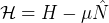$\mathstrut{\cal H} =H-\mu \hat{N}$ (with $\hat{N}$ the number operator and μ the chemical potential). However, under certain conditions such averages may be unstable with respect to an infinitesimal perturbation of the Hamiltonian. If a corresponding additive contribution $H_{\nu }\equiv \nu H^{\prime }$ of the order of ν is added ( $\nu \gtrsim 0$), i.e.,

one can define the quasi-average of A as

The average (1) and the quasi-average (3) need not coincide, since the two limits in (3) may fail to commute within some parameter region (i.e., for some combination of μ and β; $\beta =1/ k_{B}T$ being the inverse temperature).

That quasi-averages can account for cases of spontaneous symmetry-breaking can be shown by supposing that the Hamiltonian $\mathstrut{\cal H} $ displays a continuous symmetry $\mathstrut{\cal S} $, i.e., that it commutes with the generators $\Gamma ^{i}_{\mathstrut{\cal S} }$ of the corresponding symmetry group,

If some operator B is not invariant under the transformations of $\mathstrut{\cal S} $,

the (normal) average of the commutator $C^{i}$ vanishes,

by virtue of the cyclic invariance of the trace operation. However, when the perturbative part $H_{\nu }$ of (2) does not commute with $\Gamma ^{i}_{\mathstrut{\cal S} }$, this will give a nonvanishing quasi-average:

Thus, even though one might naïvely expect the quasi-average to coincide with the “normal” average in the limit $\nu \rightarrow 0$, quite generally this will not be the case. In particular, this provides a means of ‘testing’ for phase transitions: If the perturbative part of the Hamiltonian, $H_{\nu }$, is, for example, an external magnetic field that couples to the magnetization, then one can test whether a spontaneous magnetization M remains in the limit $\nu \rightarrow 0$, which would signal a phase transition to a ferromagnetic state.

This procedure generalizes to all sorts of phase transitions. The first step always consists in identifying a quantity whose (quasi-)average vanishes on one side of the transition, but takes on a finite value on the other side. This quantity is called the order parameter. For different kinds of phases, different order parameters must be chosen. Sometimes, as in the case of superconductivity, it may even be possible to characterize the same type of phase transition by use of different order parameters.

In certain cases, the relevant order parameter can be illustrated by reference to the corresponding many-body Hamiltonian. This is not surprising since many-body Hamiltonians are virtually always constructed specifically to account for certain kinds of phase transitions one is unable to derive in any straightforward way from the full theory. Consider the case of the classical Ising model proposed, in 1925, as a classical model for ferromagnetism, shortly before attention shifted towards quantum models following the realization that magnetic phase transitions cannot be accounted for by classical physics. The Ising model pictures ferromagnetism as arising from the spontaneous order of elementary magnets, which all contribute equally to the magnetization 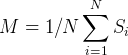$M=1/ N\sum_{i=1}^{N}S_{i}$. Since elementary magnets exert forces on each other, a coupling constant $J_{ij}$ is introduced, which gives rise to the total Hamiltonian

The Ising model was quickly dismissed, because it could not reproduce any spontaneous magnetization in the one-dimensional case of a linear chain, nor, it was conjectured (wrongly, as it turned out), in higher dimensions. However, the idea that one could construct models for many-body systems on the basis of interactions between neighboring ‘elementary magnets’, directly influenced Heisenberg's Reference Heisenberg1928 proposal of an alternative model, based on the realization that electrostatic interaction between electrons could, via a quantum-mechanical exchange mechanism, give rise to an effective spin-spin interaction—hence leading to the following quantum Hamiltonian ( $J_{ij}=J_{ji}$ and $J_{ii}=0$):

The components $S^{x}_{i}$, $S^{y}_{i}$, and $S^{z}_{i}$ of the spin $\vec{S}_{i}$ associated with each atom i, as well as the spin-raising and spin-lowering operators $S^{\pm }_{i}=S^{x}_{i}\pm iS^{y}_{i}$, are now quantum-mechanical operators which obey the usual commutator relations.

The Heisenberg model describes localized spins $\vec{S}_{i}$ of electrons located at lattice sites i in a crystal. This models the behavior of magnetic insulators, such as various Europium compounds, where the electrons cannot move about freely. A different model, to be discussed briefly in Section 4, is required for nonlocalized (‘itinerant’) electrons.

Let us summarize the main results of this section for the Heisenberg model. First, the notion of an order parameter allows for a quite general qualitative characterization of phase transitions. In the Heisenberg model, the order parameter is again the magnetization

where the factor $g_{J}\mu _{B}/ \hslash $ accounts for correct physical dimension and coupling strength and the phase factor 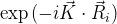$\mathrm{exp}\,(-i\vec{K}\cdot \vec{R}_{i}) $ tracks antiferromagnetic order (alternating spins) as well as ferromagnetic order (aligned spins). An external magnetic field would couple to the magnetization and thereby contribute to the Hamiltonian via the additional term $H_{b}=-B_{0}M$. (In an external field, a ferromagnet will align itself with the external field so as to minimize the energy of the system.) Whether a phase transition will occur, can then be tested—as suggested above—by looking at the spontaneous magnetization as the external field approaches zero, $B_{0}\rightarrow 0$, in the thermodynamic limit (i.e., as N, $V\rightarrow \infty $ with $N/ V=\mathrm{const}\,$).

3. Rigorous Results Concerning the Absence of Phase Transitions

The discussion of the previous section sets the agenda for how one might go about proving the existence, or absence, of a magnetic phase transition. By exploiting the properties of the Hamiltonian and by testing the system's response to an external field—later to be ‘turned off’ by taking the limit $B_{0}\rightarrow 0$—one must examine the system's magnetization M. This is not as straightforward as it sounds, due to the fact that, if the order parameter (i.e., the magnetization) has a nonzero value, then it will itself contribute a term to the Hamiltonian—precisely the term $H_{b}$ arising from the interaction with the external field $B_{0}$. Hence, we should expect to encounter an implicit equation for the order parameter. Note also that the external field $B_{0}$ can only be taken to zero once the thermodynamic limit has been carried out, since, as mentioned earlier, a phase transition is to be expected only in the thermodynamic limit.

Two aspects, however, give reason for optimism. First, quantum Hamiltonians are operators, not simple number-valued functions as in classical physics. As operators, Hamiltonians have an intrinsic mathematical structure, especially since they are so constructed as to exhibit properties that quantum theory requires of physical observables—such as their being self-adjoint—and of an energy operator in particular—e.g., its being positive definite. Exploiting such mathematical properties may allow for an independent analysis of the relation between the Hamiltonian and the order parameter. Second, the very requirement of performing the thermodynamic limit leads to a significant simplification of the problem. In a finite system, the summations that are inevitably introduced by the very structure of the Hamiltonian (namely, as a sum over lattice sites) are notoriously difficult, whereas in the thermodynamic limit they can be replaced, without loss of exactness, by continuous integrals in reciprocal space, which are much easier to handle. As it turns out, these two aspects combine to allow for the derivation of exact results concerning the possibility of magnetic phase transitions in the Heisenberg model.

The first aspect is exploited by using the Bogoliubov inequality. This relation holds between two essentially arbitrary operators A and C and a mathematical operator H with the same properties as a valid Hamiltonian of a physical system. (Not surprisingly, the operator H will normally be chosen to be the Hamiltonian.) In its original form (Bogoliubov Reference Bogoliubov1962), the Bogoliubov inequality is given by

where 〈⋯〉 denotes the thermodynamic expectation value. A and C need not have any obvious physical interpretation from the start, so the physical significance of (11) will depend crucially on the choice of operators A and C. The inequality can be proved by introducing a scalar product constructed from the energy eigenvalues $E_{n}$ as ‘weights’ and the orthogonality of the corresponding energy eigenstates $\vert n\rangle $ of the Hamiltonian H. To this artificially constructed but mathematically rigorous scalar product, one then applies the Schwarz inequality (which holds for any valid scalar product). The details of the proof are accessible elsewhere; however, we briefly note that as a result of the derivation, the two factors on the right-hand side of (11) are upper bounds to a mathematical norm and, thus, have zero as a lower bound. In particular, if, for example, the double commutator depends on some parameter, k, it will always be the case that

Dividing both sides of (11) by the double commutator and summing over all wave vectors $\vec{k}$ (which at this point is merely a vector-valued parameter, the physical interpretation of which is, strictly speaking, irrelevant), one arrives at

Written in this form, Bogoliubov's inequality suggests the following strategy: If one could find operators A, C such that the numerator of the LHS is proportional to the magnetization, it might just be possible to provide an estimate of the upper bound of the magnetization M as $B_{0}\rightarrow 0$. Of course, the Hamiltonian H in the denominator also contains a term that includes the magnetization, namely $H_{b}$. Hence, it is conceivable that for any nonzero value of M the inequality will be violated as $B_{0}\rightarrow 0$. One would then have to conclude that no spontaneous magnetization can occur.

Indeed, this is what happens when (13) is evaluated for the choice of (Fourier-transformed) operators:

By virtue of the commutation relations, one finds that

which indeed gives a contribution proportional to the magnetization on the left-hand side of the Bogoliubov inequality:

(The $\xi _{(i) }$ merely denote constants depending, at most, on fixed parameters of the many-body model, i.e., in this case the Heisenberg exchange integrals $J_{ij}$.) The other (anti-)commutators that feature in the Bogoliubov inequality can be bounded from above as shown by Mermin and Wagner (Reference Mermin and Wagner1966):

Inserting the results into the Bogoliubov inequality in its form (13) results in

As discussed earlier, the thermodynamic limit makes it possible to replace the sum by an integral without loss of exactness, e.g. in the two-dimensional case

where $L^{2}/ (2\pi) ^{2}$ is the area in k-space associated with one quantum state. Restricting the geometry of the space over which the integration is carried out in such a way that the inequality is strengthened, e.g., by limiting the integral to a finite-volume sphere inscribed into the original volume, gives

where $k_{0}$ is the cutoff corresponding to the sphere in k-space. In the thermodynamic limit under consideration, L and N approach infinity in such a way that the specific volume $v^{(2) }_{0}=L^{2}/ N$ (the inverse of the density $n^{(2) }=N/ L^{2}$) remains finite throughout. Evaluating the integral, one then arrives at

As $B_{0}\rightarrow 0$, the denominator diverges logarithmically, thus forcing the magnetization to vanish. This result is qualitatively independent of the precise parameters of the many-body model and also of the auxiliary wave vector $\vec{K}$, which accounted for antiferromagnetism. Hence the rigorous result that the two-dimensional Heisenberg model does not allow for spontaneous ferromagnetic and antiferromagnetic order—the Mermin-Wagner theorem. One can easily prove that a similar procedure rules out spontaneous magnetic order also in the one-dimensional case.

The derivation of the Mermin-Wagner theorem involves no approximation. Within the domain of the Heisenberg model and its Hamiltonian H it is as mathematically exact a result as one can hope for. Furthermore, the procedure is not limited to the Heisenberg model: Equivalent results have been derived for the Hubbard model (which describes itinerant electrons in a metal) and other quantum many-body models, for spin systems in the ‘classical’ (infinite-spin) limit, for crystalline order in classical as well as quantum systems, and for a variety of other systems. (See Gelfert and Nolting Reference Gelfert and Nolting2001 for a review of results.) In all of these cases, a phase transition in the one- and two-dimensional case is ruled out.

It is important to note that the Mermin-Wagner theorem does not have the characteristics of a law; it does not universally exclude low-dimensional phase transitions per se, but it holds rigorously for each many-body model for which it has been proven. Its derivation depends not so much on theoretical first principles, but rather on general mathematical properties of the Hamiltonian in conjunction with the choice of the order parameter. As we shall see, this is an important realization when it comes to evaluating the importance of violations of the Mermin-Wagner theorem.

4. The Mermin-Wagner Theorem vis-à-vis Levels of Approximation

How does the Mermin-Wagner theorem fit with the physics of phase transitions? One suggestion might be that the predicted absence of phase transitions in one and two dimensions is simply a spurious mathematical artefact, given that real, existing many-body systems are never truly one- or two-dimensional but finite. But note that this suggestion is difficult to square with the earlier result that for phase transitions to be at all possible within a statistical model one must consider the thermodynamic limit. If a physical system is considered ‘large enough’ for a phase transition to be expected from a thermodynamic point of view—and this surely applies to all systems that do display phase transitions in the experiment—then it should seem that consistency demands we ought also to regard the system ‘large enough’ for the thermodynamic limit to be applicable at the microscopic level of description. Yet it is precisely under these circumstances that the Mermin-Wagner theorem is valid. Recall also that the Mermin-Wagner theorem is a direct statement about the order parameter: In claiming that the order parameter cannot spontaneously take on a nonzero value, it makes a much more direct prediction than, for example, the general argument about phase transitions in finite systems, which only claims that, strictly speaking, there can be no singularities in certain thermodynamic relations. Prima facie, the mismatch between theoretical prediction and empirical data seems more curable in the latter case than in the former—after all, most physicists would not expect to be able to measure ‘singularities’ in the first place, as these will always be smoothed out one way or another.

Within the many-body models considered, however, both results seem to combine to render phase transitions thoroughly elusive: They cannot, strictly speaking, occur in finite systems, except when these are so large that they can be treated as if the thermodynamic limit were applicable; yet, when the thermodynamic limit is applicable, a rigorous argument rules out phase transitions in one and two dimensions. It is of little help to appeal to the fact that most ‘low-dimensional’ ( $D< 3$) physical systems are really layered structures that extend into the third dimension or, at the very least, are embedded into three-dimensional space. For, as has been shown in Gelfert and Nolting Reference Gelfert and Nolting2000, the argument for the Mermin-Wagner theorem still goes through, for any finite number d of layers. It even extends to fractal systems whose (spectral) dimension cannot be identified with any Euclidean spatial dimension.

Given the variety of many-body systems for which the Mermin-Wagner theorem has been shown to hold, there appears to be no obvious way to blame the failure to account for—empirically observed—low-dimensional phase transitions on the structure of the Hamiltonian, either. This is not to say that the models defined by these Hamiltonians aren't approximations—they were introduced precisely as simplified models for the intractable full many-body problem. Yet physicists tend to place a great deal of trust in well-established models, especially when these can be given a direct physical interpretation. Consider, for example, the Hubbard model:

Here, the operators are not spin operators but creation and annihilation operators $c^{+}_{i\sigma }$, $c_{i\sigma }$, and number operators $n_{i\sigma }$ of an electron of spin σ at lattice site i in the crystal. The Hamiltonian can also be derived explicitly using the formalism of second quantization; its overall structure guarantees conformity to certain basic laws, such as the Pauli principle. The interpretation of the first term of the Hubbard Hamiltonian is straightforward: The first operator,Footnote ¹ $c_{j\sigma }$, annihilates an electron of spin σ at site j, and the second operator, $c^{+}_{i\sigma }$, creates an electron of the same spin at site i; in other words, a σ-electron jumps from one lattice site to another, which is how the model describes itinerant electrons. The second term accounts for the fact that at each lattice site, two electrons, one with spin-up and one with spin-down, can coexist. If an electron is already in place ( $n_{i\sigma }=1$), then, if a second electron is to be placed at the same lattice site, a price has to be paid in terms of energy, U, due to the electrostatic Coulomb force between the two electrons. Any modification of the Hamiltonian specifically designed to give a phase transition in low dimensions would need to be backed up by a similarly intuitive interpretation in order to avoid being ad hoc. Interestingly, this is not what physicists typically try to do. Instead, they analyze the corresponding many-body models using numerical techniques or analytical approximations.

Such approximations may take the form of computer algorithms or recursive analytical methods which approximate the exact quantum-mechanical equations of motion. Importantly, these methods are approximations of the mathematical problem represented by the many-body model, and hence, at the level of physical theory, are second-order approximations: They approximate models which themselves were introduced as approximations of the full many-body problem (e.g., the problem of ferromagnetism in EuO). Frequently, these methods ‘violate’ the Mermin-Wagner theorem, in that they do predict phase transitions even in two dimensions. Such violations raise a pressing question: How can one rely on numerical results derived from a model using a variety of approximative methods, when one of the few exact results about the model is that none of the sort of behavior suggested by the numerical results should occur? Surprisingly few researchers have commented on this problem. Occasionally the breaking of the Mermin-Wagner theorem has been taken to be an instrumental advantage; Sukiennicki and Wojtczak (Reference Sukiennicki and Wojtczak1972, 37), for example, believe “that the molecular field approximation [which violates the Mermin-Wagner theorem] approaches the physical reality (magnetic order in thin films does really exist) better than the Hubbard model in its exact form.” While this may seem prima facie justified, at least for the pragmatic purpose of describing occurrent physical phenomena, other physicists have dismissed such nonchalance with regard to exact results: “[A]pproximation schemes that have been applied to real solids can equally well be applied to one- and two-dimensional solids. If these approximation schemes predict the occurrence of spontaneous magnetization in one and two dimensions as well as in three dimensions …, the validity of these predictions in three dimensions should clearly be investigated more fully” (Walker and Ruijgrok Reference Walker and Ruijgrok1968, 515). The reasoning seems to be as follows: If one aspires to formulate criteria for the reliability of one's methods of approximation (rather than proceed in an ad hoc fashion), then one will need to shed some light on the relation between the underlying many-body model, the exact results known about it, and the mechanism of approximation. In other words, it would be unsatisfactory to rely blindly on the method of approximation's introducing exactly the kind of symmetry-breaking needed to reflect physical reality.

5. The Interpretative Flexibility of Exact Results

The existence of a rigorous proof of the absence of phase transitions, in conjunction with the empirical success of approximative methods violating these exact results, poses a genuine puzzle to the theoretician. Quantum many-body Hamiltonians have been investigated in part because it was realized that collective magnetism could not be explained within the framework of classical physics. The Bohr-van Leeuwen theorem rules out spontaneous magnetic order tout court for systems governed by classical electrodynamics—no matter what the system's dimension. This being so, would it then be rational to accept an impossibility theorem such as the Bohr-van Leeuwen theorem, but reject the equally rigorous Mermin-Wagner theorem in order to save the predictions of one's approximations? This hardly seems a viable option.

But perhaps the comparison is not quite fair. Whereas the Bohr-van Leeuwen theorem can be proved solely from first principles—the laws of electrodynamics and the classical Hamiltonian function—the Mermin-Wagner theorem holds for specific Hamiltonians, which themselves represent only part of the full problem. This does not render the Mermin-Wagner theorem any less rigorous within the limits of the corresponding many-body model, but it may cast doubt on the theorem's physical significance. If the theorem's mathematical validity is beyond doubt, perhaps one can blame the choice of the model for the mismatch between the empirical reality of phase transitions and their predicted absence? In practice, however, this is not an option seriously pursued by physicists, since, as mentioned earlier, several of the many-body models have become objects of study in their own right—particularly in mathematical physics. Also, it is unclear which additional criteria could usefully guide one's choice of many-body models. As the multiplicity of different kinds of many-body models indicates, many possible modifications have been explored and they all conform to the Mermin-Wagner theorem. Simply postulating that the full theory, in its state of innocence before the introduction of reduced many-body Hamiltonians, would explain the empirical data, if only we were able to spell out and solve it, expresses nothing but a leap of faith. Such a move would also ignore the vital role that models play in science. As the earlier example of the Hubbard model showed, it is typically at the level of models that theoretical desiderata such as intuitiveness and simplicity are assessed and explanations of physical phenomena are tested.

If blind faith in fundamental theory is at one end of the spectrum, the instrumentalist attitude displayed by Sukiennicki and Wojtczak is at the other end. According to this view, whatever numerical methods of approximation generate (approximately) true predictions should be instrumentally acceptable. This, however, appears to get the order of dependence wrong: The numerical methods in question are approximations of the model, and as such they contain no more information than the original many-body model. The contribution of an approximation is wholly negative, in that it leaves out and ignores information that cannot readily be extracted from the model—for, if it could, then the model would be exactly solvable and no approximation would be necessary in the first place. Whatever an approximation leaves out is beyond our control. This is what makes it so difficult to credit approximations with ‘breaking the symmetry’, that is, with reliably predicting the occurrence of a phase transition in cases where the model predicts an absence. For, it seems awkward to derive justification for our results from that part of the process that we cannot know—that is, the error term introduced by the approximation—rather than from what we do know, i.e. the model.

If one accepts that neither instrumentalism nor theoretical fundamentalism succeed in eliminating models from the process, the dilemma posed by the Mermin-Wagner theorem re-emerges in even greater clarity. Remember that the derivation of the Mermin-Wagner theorem is for the most part a mathematical exercise and does not draw on theoretical notions that are not already presupposed in formulating the model! (The notion of presupposition here is not meant to imply that the model is derived from high-level theory, but rather that some theoretical notions and inferential methods are required to make sense of the model quite independently of high-level theory.) The important question then is which attitude is needed to resolve the tension between, on the one hand, the ineliminability of models and, on the other hand, their unavoidable limitations, as exemplified by the empirical refutation of the Mermin-Wagner theorem. What this calls for, I believe, is a middle path between instrumentalist nonchalance and theoretical fundamentalism. What is required is, so to speak, a commitment to ‘being realistic’—in the sense of being modest in one's expectations—about both exactness and apparent inconsistency.Footnote ² The search for qualitatively and numerically satisfactory accounts of phase transitions in many-body models is as well-established a research project as one can hope to find in physics. The results and models derived within this domain of inquiry have reached a high degree of stability and accuracy. In such cases, where we have a reliable track record of improvements, refinements and empirical confirmation at various theoretical and experimental levels, the persistence of an inconsistency or, more cautiously, of a mismatch—such as that between the exact Mermin-Wagner result and the prediction of low-dimensional phase transitions derived from the same models via approximations—need not lead to an implosion of the research project.

Previous authors have focused on inconsistencies between theories (for example between a predecessor and a successor theory in cases of theory change) or within the axiomatic structure of a theory (as in the case of Bohr's theory of spectral emissions). (See Smith Reference Smith1988.) One line of argument has been to advocate relaxing one's standards of consistency and embrace inconsistency by adopting a framework of paraconsistent logic.Footnote ³ Such approaches, however, remain highly controversial, and, at least in the present case, would seem quite extravagant. What is at stake in the case of the Mermin-Wagner theorem is not the consistency of the underlying theory but rather the uses to which certain strategies of modeling and numerical evaluation are put. This kind of inconsistency, to put it somewhat elliptically, is performative rather than theoretical. What is called for is not so much a revision of one's logical framework as taking seriously the suggestion that acceptance of a theory or model must be properly contextualized. The proper object of epistemic evaluation is a model in conjunction with a numerical method of approximation, where the acceptability of the latter is itself determined by a host of criteria beyond mere numerical success.

Scientists, more often than not, are dealing with a hierarchy of commitments, ranging from (perhaps dispensable) belief in merely contingent facts to (essential) guiding principles underlying the fundamental theory or model. (See also Da Costa and French Reference Da Costa, French, French and Kamminga1993.) Not all of these commitments are on a par with one another and, consequently, not all ‘inconsistencies’ are equally disastrous. Indeed, in the Mermin-Wagner case, the idea of a hierarchy of commitments is especially attractive. As mentioned earlier, the Mermin-Wagner theorem does not have the status of a fundamental law. Even though it holds for all standard many-body models, its validity must be demonstrated anew for each model Hamiltonian. By way of contrast, the Pauli principle is a law of nature and, as described earlier, its validity is both presupposed in the construction of the many-body model and guaranteed by the formal (i.e., ‘second-quantized’) structure of the Hamiltonian. Hence, while violations of the Pauli principle—which do occur in certain numerical approximations—indeed threaten to introduce inconsistencies with the model's premises (and, for this reason, are strongly rejected; see Keiter and Kilić Reference Keiter and Kilić1998), the Mermin-Wagner theorem is much more on a par with other contingent results flowing from the model, and may well ‘lose out’ against competing factors and desiderata.

While this may not amount to a universal theory of inconsistency in science, it does cast some light on the role of exact results in a great number of contexts. After all, ‘being realistic’ about inconsistencies in such cases must also entail ‘being realistic’ (in the sense of ‘being modest’) about the status of exact results. Enforcing conformity with exact results at the expense of the cohesion and explanatory power of the carefully crafted patchwork of theoretical models and numerical techniques may just become too costly at some point. Indeed, this seems to be the most attractive way of dealing with the curious ‘mismatches’ between exact results and numerical predictions that one encounters in the case of many-body models, and it seems, on the whole, that this is also the preferred way theoreticians themselves treat exact results: Sometimes they may ignore or dismiss them in a hasty fashion, but sometimes they do appeal to them as benchmarks for new methods of approximation.