Two-Stage Optimal Control Technique

Summarizing the discussion just before, our optimal control problem is

subject to (1) and (2), K₀ given, and K(T)≥0 free. Note that we can rewrite our objective function as follows:

Because the welfare performances of the two possible technological regimes are additively separable, the use of two-stage optimal control is most natural. The approach is carefully described and theoretically founded in Tomiyama (1985) and Tomiyama and Rossana (1989). An extension to infinite-horizon programs has been very recently provided by Makris (2001). As mentioned in the introduction, the method proceeds by solving a sequence of conventional Pontryagin problems. In our case, the sequence contains two problems, which corresponds to the number of possible technological regimes, but as will be clear in a moment, the method should work at least for any finite number of problems [see Saglam (2002)]. Applied to our model, the method works like this:

Step 1. New-technology problem. Assume that the economy does switch to the new technology at t₁. Furthermore, assume also that initial capital stock for the new technology K(t₁)=K₁ is given. For t₁ and K₁ given, maximize

, subject to the state equation (2)—

, t₁<t≤T— with K(T) free. Denote by λ₂(t) and by H₂(K, C, t, λ₂)=−u[C(t)]e^−ρt+λ₂[q₂A₂K(t)−q₂C(t)], respectively, the costate variable and the Hamiltonian associated with this Pontryagin problem.⁵

Step 2. Old-technology problem. Maximize

, subject to the state equation (1)—

, 0≤t<t₁—K₀ given and K₁=K(t₁) free. This is done in two substeps:

1. Solve the problem for fixed K₁ and t₁, with λ₁(t) and H₁(K, C, t, λ₁)=−u[C(t)]e^−ρt+λ₁[q₁A₁K(t)−q₁C(t)], respectively, the corresponding costate variable and the Hamiltonian. Denote by H*₁(K₁, t₁) the resulting optimal Hamiltonian value.
2. Matching conditions: Continuity and optimality. Find the optimal values for K₁ and t₁. For interior optimal solutions, K*₁ and t*₁, to exist, the following equations should hold:
   
   If U₂(K₁, t₁) is twice continuously differentiable in K₁ and t₁, these conditions become
   

As one can easily see, equation (6) featuring the optimality of the K₁'s choice ensures the continuity of the costate variable at t₁. Equation (7) is the optimality condition for an interior switching time to exist.

Step 3. Sufficient condition for maximum.

Step 4. Corner solutions. Assume that U₂(K₁, t₁) is twice continuously differentiable in K₁ and t₁, which turns out to be the case in all our applications. Consider the case where the equations (6)–(7) have no solution in t₁ such that 0<t₁<T. Two corner solutions are still possible.

1. Immediate switching: t*₁=0 if H*₁(K₀, 0)≥H*₂(K₀, 0).
2. Technological sclerosis: The economy will never switch in the time interval [0 T] if and only if H*₁(K*₁, t*₁)<H*₂(K*₁, t*₁) for every t₁ in [0 T] and H*₁[K*(T), T]≤H*₂[K*(T), T].⁶

   Since time is continuous, the corner solution

   also features technological sclerosis.

We apply this method to our basic model and give the details of the corresponding computations in the next section. The algebraic details are omitted in further applications of the method.

Solving the Model

We will follow closely the method described above starting with the solution of the Pontryagin problem corresponding to the new technological regime. We take the logarithmic utility case to ease the exposition; the method still produces closed-form solutions for any other isoelastic utility function, for example. Concise economic interpretations follow the technical exposition.

Step 1. Our optimal control problem is

subject to

, with K₁ given and K(T)≥0 free. With the corresponding Hamiltonian defined as H₂(K, C, t, λ₂)=−u[C(t)]e^−ρt+λ₂[q₂A₂K(t)−q₂C(t)], the first-order necessary conditions are standard:

and with

Since C* clearly depends on the choice of t₁ and K₁, it is obvious that U*₂=U*₂(K₁, t₁). The (trivial) integration of these necessary conditions gives us the following results

Given the terminal point condition (11), one may find that

Thus, at t₁, we have

This finally allows us to compute the optimal welfare performance of the new technology regime in terms of t₁ and K₁:

Notice that U*₂(K₁, t₁) is trivially twice differentiable with respect to both K₁ and t₁. Accordingly, one can check that the following relations hold:

Step 2. Now we have to solve the following Pontryagin problem:

subject to

, 0≤t<t₁, with K₀ given and K₁=K(t₁) free. Assuming that t*₁ is an interior point in [0, T] makes the constraint 0≤t₁≤T inactive and we are left with an auxiliary problem for the old technology with free endpoint and free terminal time.

1. For fixed t₁ and K₁, the Pontryagin maximum principles allow us to write straightforwardly the first-order conditions as in step 1. Integrating them gives
   
2. To determine optimal K₁ and t₁, we use the continuity and optimality conditions (6) and (7). By means of (6), we can find that
   
   Thus, at t₁, we have
   
   Now, utilizing the optimality condition (7), we can determine the (interior) optimal time of switching to the new technology as follows:
   
   It follows that there exists an interior solution such that 0<t*₁<T for a given T>0, if and only if
   

Step 3. We check the second-order condition to see whether t*₁ leads to a maximum or not. For t*₁ to be a welfare-maximizing switching time, a sufficient condition is that, at t*₁,

Therefore,

Note that this violates the condition under which an interior solution exists such that 0<t*₁<T for a given T>0. The date t*₁ computed in step 3 is not a maximizer.

Step 4. We finally investigate under which parametric conditions the corner solutions arise. Since q₂>q₁, the condition just above can be broken in two ways.

1. Technological sclerosis: If q₂A₂−q₁A₁≤0, the interior solution does not exist. Indeed under this condition, we always have H*₂(K₁, t₁)−H*₁(K₁, t₁)>0 for every 0≤t₁≤T as long as q₂>q₁. This implies that there is no incentive to switch in such a case. If q₂A₂−q₁A₁>0 but
   , we still have H*₂(K₁, t₁)−H*₁(K₁, t₁)>0 for every 0≤t₁<T, and H*₂(K_T, T)−H*₁(K_T, T)≥0: Switching is not optimal either.
2. Immediate switching: If t*₁=0, then H*₁(0)≥H*₂(0). Therefore,
   
   or
   

Note that, from the parametric conditions under which we obtain corner solutions, switching to the new technology with a delay is always dominated by either switching immediately or sticking to the old technology alternatives.

Economic Interpretation

We now concisely interpret the results above. We summarize them in the following proposition.

PROPOSITION 1. Assume q₂>q₁ and A₁>A₂.

1. If q₂A₂−q₁A₁≤0, the economy will not switch to the new technology.
2. If q₂A₂−q₁A₁>0, then

1. either
   
   and the economy immediately switches to the new technology;
2. or
   
   and the economy sticks to the old technology;
3. or
   
   and the economy is indifferent between switching or sticking.

These results come from some specific outcomes of the embodiment assumption. To understand them easily, note that from our computations in the preceding section, optimal consumption follows the path

if 0≤t<t₁, and

for t₁<t≤T, with α and β two constants such that α/β=q₂/q₁. Equation (27) is obtained by combining (13), (15), and (16), and (28) is obtained by combining (21), (23), and (24). Notice the two following characteristics of optimal consumption:

Let us further interpret property (P₁). The acceleration in the rate of embodied technological change is associated in our framework with a reduction in the relative (shadow) price of capital. In other words, this acceleration is accompanied by a rise in the (shadow) price of consumption goods with respect to the (shadow) price of capital goods. This induces a reassignment of the resources of the economy toward the capital-goods sector, resulting in relatively less consumption and more capital accumulation. So, the consumption level should drop from the date of the switch. Since the utility function is logarithmic here, the welfare cost of this drop is ρln(q₂/q₁). The higher the impatience rate ρ, the bigger the welfare cost due to the drop in the consumption level. We refer in this cost as the the obsolescence costs inherent in embodiment as it derives from the decrease in the relative (shadow) price of capital.

On the other hand, if the economy switches to the new regime and if the resulting improvement in the efficiency of capital goods is enough to compensate for the loss in expertise, the economy will experience a higher growth rate. The growth rate differential is q₂A₂−q₁A₁>0. Because the horizon is finite, the growth-rate advantage is exactly (1−e^−ρT)(q₂A₂−q₁A₁). As T shrinks, this advantage gets smaller. The trade-off is clear and can be measured by the ratio cost to advantage of switching,

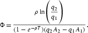
If Φ>1, the economy has no incentive to switch [case (b)(ii) of Proposition 1]: The obsolescence costs more than compensate for the growth advantage from switching. If, in contrast, Φ<1, the economy should switch immediately because the growth advantage is the dominating force in such a case.

Notice that in this benchmark model, delaying technology adoption is never optimal, even when the obsolescence costs coming from switching are close to the corresponding growth advantage (Φ slightly lower than 1). The rationale behind this behavior is the following.⁹

Infinite-Horizon Case

In this section, we study the infinite-horizon extension of our benchmark model, T=∞. One may follow exactly the computation steps detailed in our application to the benchmark model. This is not necessary if one has in mind that the solution paths of the infinite-horizon problems are likely to be the limits of the solution paths obtained in the finite-horizon case when T tends to infinity. Indeed, the optimization horizon crucially enters step 1 of the method, the so-called new-technology Pontryagin problem. In particular, the terminal conditions (11) are very important: λ*₂(T)≤0 and K*(T)λ*₂(T)=0. Since the objective function of our problem is strictly concave in the control variable and since it is discounted, the needed transversality conditions are just the limits of the terminal conditions (11) when T goes to infinity:

with

. As one can check, this is the unique departure with respect to the benchmark case, in steps 1 and 2(i). In particular, the optimal consumption path follows a similar motion:

if 0≤t<t₁, and

for t₁<t, with α′ and β′ two positive. Again, one can check that, as in the benchmark case, α′/β′=q₂/q₁. Again, we have property (P₁): An acceleration in embodied technical progress induces a drop in the consumption level. How does the growth-rate advantage of the new regime play now? Recall that in the finite-horizon case, this advantage is captured by the term (1−e^−ρT)(q₂A₂−q₁A₁). In the infinite-horizon case, this advantage is simply q₂A₂−q₁A₁. If q₂A₂−q₁A₁≤0, then there is no incentive to switch. What happens if q₂A₂−q₁A₁>0? Is there any way to generate interior switching time? Our economic interpretations in the last paragraph of Section 2.3 suggest a negative answer to this question. Either with a finite-or an infinite-time horizon, consumption discontinuities are not optimal after t=0 under perfect foresight and strictly concave preferences. This diagnosis is confirmed by the method. Indeed, closely following step 2(ii) of the method, one ends up with the following expression for H*₂(K₁, t₁)−H*₁(K₁, t₁):

For an interior solution to exist, we must have H*₂(K₁, t₁)−H*₁(K₁, t₁)=0. A quick look at the expression above is sufficient to see that the latter equation (in t₁) is degenerate. We then trivially identify the following cases.

PROPOSITION 2. Assume q₂>q₁ and A₁>A₂.

1. If q₂A₂−q₁A₁≤0, the economy will not switch to the new technology.
2. If q₂A₂−q₁A₁>0,

1. then
   
   the economy switches immediately to the new technological regime;
2. or
   
   the economy sticks to the old technology.¹⁰

   In the equality case,

   

   the economy is indifferent between switching and sticking. We abstract from this case hereafter.

Hence, independently of whether the optimization time horizon is infinite, only two decisions might be optimal and both are corner solutions: either immediate switching when the obsolescence costs are lower than the growth-rate advantage of switching [case (b) (i) of Proposition 2], or sticking to the old technology in the reverse situation [case (b) (ii) of Proposition 2]. We next examine a much richer model including learning and incentives to wait.

Solving the Model

Step 1. The Pontryagin conditions corresponding to the new technology problem are (9) and (10) as before, with the transversality conditions lim_t→∞K*(t)λ*₂(t)=0 and lim_t→∞λ*₂(T)≤0. The corresponding Hamiltonian is

Integrating the Pontryagin conditions, one finds after some trivial but heavy algebra that

Finally, the transversality conditions give

Now come the new things with respect to the benchmark-case application. Using the expressions above for optimal consumption, capital accumulation, and the costate variable, one can again express the optimal value of the objective function as a function U₂(K₁, t₁). It is then possible to check that

With respect to the benchmark case, a new term appears in the expression of

, namely

. This term captures the effects of a change in the switching date on the Hamiltonian value, and so on the optimal welfare performance of the second technology regime. It is present here because the switching-date value affects explicitly the pace of capital accumulation through the learning costs. This new term will obviously appear again in the matching conditions in step 2(ii).

Step 2.

1. Since H₁(K, c, t, λ₁)=−ln[C(t)]e^{−ρ t}+λ₁q₁[K(t)−C(t)], this step is identical to step 2(i) in Section 2.2. So, equations (20), (21), and (22) still hold with A₁=1. In particular, we get
   
   where
   is the integration constant.
2. The optimality condition of the problem with respect to K₁ does not change; equation (4) still applies. However, since t₁ appears directly in the accumulation law of capital along the second technological regime, a new optimality condition arises with respect to t₁:
   
   Using the results of step 1, one can check that this condition can be rewritten as
   
   while, as in the benchmark case, equation (6), the optimality condition with respect to K₁ may be rewritten as a continuity requirement at t=t₁ of the costate variable. From this continuity condition,
   , one can compute the integration constant
   as
   , which allows one to derive the optimal paths of consumption, capital accumulation, and the costate variable in terms of t₁. In particular,
   . Substituting in the (interior) optimality condition with respect to t₁, namely, in equation (34), one gets, after some trivial but cumbersome algebraic operations, that
   
   One can easily check that optimal t*₁∈(0, ∞) if and only if
   

Step 3. The sufficient condition for

to be welfare maximizing is

which can be recast as

It can be easily checked that at

, given by (35), the sufficient condition reduces to

which is always satisfied.

Step 4. The necessary conditions for the degenerate cases, where either the optimal switching appears immediately or switching never occurs can be found very easily.

1. Technological sclerosis: This case occurs if
   if t*₁→∞. This happens if and only if the following condition holds:
   
2. Immediate switching: The economy switches immediately if
   when t*₁=0. The corresponding parametric condition is
   

Economic Interpretations and Comparative Statics

Denote by

The results of the previous section can be summarized by the following proposition.

PROPOSITION 3. Assume q₂>q₁.

1. If 0<Δ<[bq₂(κ+ρ)]/(θ+ρ), then adoption is delayed, the optimal switching date
   being given by (35).
2. If Δ≤0, the economy should stick to the old technology.
3. If Δ≥[bq₂(κ+ρ)]/(θ+ρ), the economy should switch immediately to the new technology.

To improve the readability of our mathematical results and their economic discussion, we state the optimization outcomes in the special case where the amount to be learned is constant, that is, b=0.

COROLLARY 1. Under q₂>q₁, if b=0, then either technological sclerosis or immediate switching occurs:

As in the benchmark case, we have again to deal with the obsolescence costs and growth advantages of adopting a new technology with a higher level of embodied technological progress. Obsolescence costs are still measured by ρln[q₂/q₁]. Indeed, the optimal consumption path is given by

and

Taking the one-sided limits of the consumption path at t₁ is enough to see that the obsolescence costs, at the basis of the drop in the level of consumption, can be measured exactly as in the benchmark case by ρln[q₂/q₁]. The growth advantage of switching is now measured by q₂−q₁ since both regimes imply the same long-term marginal productivity of capital, equal to 1. Nonetheless, for this to hold, the economy should “learn” once it switches, and this is costly. Now, recall the learning-curve structure:

, for t₁<t, with

. The amount to be learned, A^{[sstarf ]}, consists of two different terms. The first one related to

does depend on the value of t₁ and represents a kind of value option of waiting. By choosing t₁, the economy indeed controls this component of the learning process. The second term related to α₀(q₂/q₁) does not depend on t₁ and captures the fixed learning costs. The economy has no control on this term: It exclusively depends on the intrinsic characteristics of the two considered technological menus, and, as such, this term is not “manipulable” by the potential adopters. The indicator Δ, constructed above, is consequently the growth advantage of switching net of the obsolescence costs and the fixed switching costs. Obviously, if Δ≤0, the economy has no incentive to switch [case (ii) of Proposition 3].

When Δ>0, the economy will switch. If Δ is big enough to “compensate” for the option of waiting, namely, the term [bq₂(κ+ρ)]/(θ+ρ), then there is no reason to wait, and the economy will switch immediately [case (iii) of Proposition 3]. Otherwise, the economy will wait, and a strictly positive adoption delay will arise [case (i) of Proposition 3]. If the amount to be learned is constant (Corollary 1), the value option of waiting is nil, implying that an interior switching time is never optimal. In such a case, the cost of switching technologies is simply increased with respect to the benchmark model. Learning costs add to the obsolescence costs: There is no substantial departure from the benchmark model, and the economy either “sticks” or immediately switches.

What are the determinants of the optimal adoption delay if it arises? The next proposition summarizes the results regarding this aspect.

PROPOSITION 4. Assume that 0<Δ<[bq₂(κ+ρ)]/(θ +ρ), so that switching is delayed,

being given by equation (35). Then,

and

. In contrast, the sign of

is ambiguous. A sufficient condition for

to be positive is ρ<(1−θ)/2.

The properties stated in the proposition come from the expressions of the derivatives. Indeed,

because both the denominator and the numerator inside the brackets are positive (due to the existence of interior-switching). This is far from surprising. A higher value for θ means a faster learning process, which increases the incentives to switch. On the other hand, one immediately gets

where α₀ measures the sensitivity of the fixed learning costs to the magnitude of the technological acceleration as captured by the ratio q₂/q₁. Thus, an increase in α₀ raises the fixed costs of learning and discourages switching. In contrast, the behavior of adoption timing with respect to time discounting is again ambiguous.

In effect,

The denominator inside the brackets is positive due to the condition ensuring the existence of an interior switching date. The sign of the numerator is ambiguous. A rise in ρ increases the obsolescence costs, ρln[q₂/q₁], which tends to delay adoption. However a more “impatient” economy would also accelerate adoption since the sooner the adoption, the sooner the economy will start to learn and the quicker it will gain expertise in the new technology. This aspect is captured by the term θ+ρ in (35), for example. Therefore, the adoption delay is a very complex function of the impatience rate. A sufficient condition for

is that ρ<(1−θ)/2. If the learning speed is very low (i.e., θ tends to zero), this condition is checked by far for reasonable values of the impatience rate. In such a case, the obsolescence cost effects dominate the learning incentive, and the adoption delay is increased.