1 Introduction
Rapidly rotating atmospheres behave like quasi-two-dimensional fluids, in which an upscale transfer of energy results in the formation of large-scale patterns (Charney Reference Charney1971). For example, zonally banded structures commonly referred to as ‘alternating jets’ are seen in the atmospheres of Jupiter and Saturn (Beebe et al.
Reference Beebe, Ingersoll, Hunt, Mitchell and Müller1980; Gierasch, Conrath & Magalha Reference Gierasch, Conrath and Magalha1986; Read et al.
Reference Read, Conrath, Fletcher, Gierasch, Simon-Miller and Zuchowski2009). In such atmospheres, the upscale transfer of energy (see Young & Read Reference Young and Read2017), supplied by baroclinic instabilities and small-scale convection due to internal heating, leads to an alternating jet pattern. Rhines (Reference Rhines1975) first proposed a mechanism for jet formation, in which the upscale energy transfer is modified by the presence of Rossby waves (i.e. the ‘
 $\unicode[STIX]{x1D6FD}$
-effect’ due to Coriolis parameter meridional gradient
 $\unicode[STIX]{x1D6FD}$
) and channelled into zonal structures. The presence of alternating jets has been confirmed in a variety of eddying nonlinear model solutions (Williams Reference Williams1979; Panetta Reference Panetta1993; Vallis & Maltrud Reference Vallis and Maltrud1993; Cho & Polvani Reference Cho and Polvani1996; Huang & Robinson Reference Huang and Robinson1998; and others) and it has been observed that the meridional width of the jets is controlled by the magnitude of
 $\unicode[STIX]{x1D6FD}$
and the eddy energy (Rhines Reference Rhines1975; Maltrud & Vallis Reference Maltrud and Vallis1991; Vallis & Maltrud Reference Vallis and Maltrud1993; Scott & Polvani Reference Scott and Polvani2007; Sukoriansky, Dikovskaya & Galperin Reference Sukoriansky, Dikovskaya and Galperin2007; Chemke & Kaspi Reference Chemke and Kaspi2015a
).
More recently, oceanic multiple alternating jets (sometimes referred to as ‘latent jets’ or ‘striations’) have been observed in satellite altimetry, float datasets and eddy-resolving ocean general circulation models (Maximenko, Bang & Sasaki Reference Maximenko, Bang and Sasaki2005; Nakano & Hasumi Reference Nakano and Hasumi2005; Richards et al.
Reference Richards, Maximenko, Bryan and Sasaki2006; Sokolov & Rintoul Reference Sokolov and Rintoul2007; Van Sebille, Kamenkovich & Willis Reference Van Sebille, Kamenkovich and Willis2011; Cravatte, Kessler & Marin Reference Cravatte, Kessler and Marin2012; Buckingham & Cornillon Reference Buckingham and Cornillon2013; Cravatte et al.
Reference Cravatte, Kestenare, Marin, Dutrieux and Firing2017). There is general agreement that at leading order the oceanic jets can be explained by quasi-geostrophic (QG) dynamics with the
 $\unicode[STIX]{x1D6FD}$
-effect (Kramer et al.
Reference Kramer, van Buren, Clercx and van Heijst2006; Nadiga Reference Nadiga2006). However, ambiguities remain about their generation mechanisms, the relative importance of the barotropic and baroclinic modes, and the interactions between the jets and eddies. Jet formation may be predicted by the stochastic structural theory in the
 $\unicode[STIX]{x1D6FD}$
-plane barotropic turbulence (Farrell & Ioannou Reference Farrell and Ioannou2007; Marston, Conover & Schneider Reference Marston, Conover and Schneider2008; Srinivasan & Young Reference Srinivasan and Young2012; Constantinou, Farrell & Ioannou Reference Constantinou, Farrell and Ioannou2014). Alternatively, Berloff (Reference Berloff2005b
) and Berloff, Kamenkovich & Pedlosky (Reference Berloff, Kamenkovich and Pedlosky2009a
,Reference Berloff, Kamenkovich and Pedlosky
b
) explained the jet formation in terms of interacting multiscale eigenmodes and non-local energy transfers to zonal eigenmodes, and further argued that the width of the jets is controlled by the first baroclinic deformation radius. Furthermore, Berloff & Kamenkovich (Reference Berloff and Kamenkovich2013a
,Reference Berloff and Kamenkovich
b
) showed that, despite the essential nonlinearity, the jets and eddies are significantly controlled by underlying linear dynamics. It is argued that the jets can be explained by spatially inhomogeneous stirring of potential vorticity (PV) that results in a ‘staircase’ structure of the meridional PV profile (see figure 5 in McIntyre Reference McIntyre1982), where the jets reside at the PV interfaces (Baldwin et al.
Reference Baldwin, Rhines, Huang and McIntyre2007; Dritschel & McIntyre Reference Dritschel and McIntyre2008; Dunkerton & Scott Reference Dunkerton and Scott2008). Other factors such as instability of meridional boundary currents (Hristova, Pedlosky & Spall Reference Hristova, Pedlosky and Spall2008; Wang et al.
Reference Wang, Spall, Flierl and Malanotte-Rizzoli2012), secondary or modulational instability of Rossby waves (Berloff Reference Berloff2005b
; Connaughton et al.
Reference Connaughton, Nadiga, Nazarenko and Quinn2010; Qiu, Chen & Sasaki Reference Qiu, Chen and Sasaki2013) and bottom topography (Sinha & Richards Reference Sinha and Richards1999) can also induce multiple alternating jets.
In this paper, we explore the effects of bottom topography on oceanic baroclinic jets, eddies and their dynamics. In particular, transient braided jets steered by topography have been found in many situations (Sokolov & Rintoul Reference Sokolov and Rintoul2007; Thompson Reference Thompson2010; Thompson & Richards Reference Thompson and Richards2011; Chen, Kamenkovich & Berloff Reference Chen, Kamenkovich and Berloff2015). The jet transport properties also tend to be significantly different in the presence of topography. For example, with a two-dimensional topography, the meridional eddy-induced transport increases with increasing topographic steepness because of induced non-zonal mean flows (Thompson Reference Thompson2010; see also Tréguier & Panetta Reference Tréguier and Panetta1994). While studying the effects of zonally sloping topography, Boland et al. (Reference Boland, Thompson, Shuckburgh and Haynes2012) found that jets drift meridionally and tilt with respect to the zonal direction at an angle that increases with the zonal component of PV gradient. Tilted and drifting jets have also been found in Argo float data and comprehensive ocean circulation models (Nakano & Hasumi Reference Nakano and Hasumi2005; Van Sebille et al. Reference Van Sebille, Kamenkovich and Willis2011; Stern, Nadeau & Holland Reference Stern, Nadeau and Holland2015; Chen, Kamenkovich & Berloff Reference Chen, Kamenkovich and Berloff2016). It has been shown that the jets tilt towards the tilted isolines of the mean barotropic PV (Boland et al. Reference Boland, Thompson, Shuckburgh and Haynes2012). However, there is no clear explanation of why the jets drift. Boland et al. (Reference Boland, Thompson, Shuckburgh and Haynes2012) and Chen et al. (Reference Chen, Kamenkovich and Berloff2016) hypothesise that the drift is controlled by linear dynamics. Thompson & Richards (Reference Thompson and Richards2011) and Chen et al. (Reference Chen, Kamenkovich and Berloff2015) studied the dynamics of jets in the presence of meridional ridges. They found that the jets, which are present downstream of the ridge, are pushed in the meridional direction because of offset nonlinear eddy forcing.
In this work, we specifically concentrate on the drifting behaviour of multiple alternating jets in baroclinic eddying flows. Similar to Boland et al. (Reference Boland, Thompson, Shuckburgh and Haynes2012), a simple topography is considered that increases linearly in the zonal direction. The effects of the resulting zonal asymmetry on the dynamics of alternating jets are studied in a two-layer QG model forced with a horizontally uniform, zonal, vertical shear. Statistically equilibrated nonlinear flow solutions show the presence of meridionally drifting tilted jets, as in Boland et al. (Reference Boland, Thompson, Shuckburgh and Haynes2012). The drift velocities are then compared with predictions from the linear dynamics. In the later part, we use a non-stationary, tilted frame of reference to study the nonlinear and linear stress terms in the time-averaged dynamical balances, as well as their correlations with the mean PV. The nonlinear eddy forcing is further decomposed into the Reynolds stress term and form stress term, and their roles in the maintenance of the jets are investigated. Eddy fluxes of relative vorticity and buoyancy are also analysed. The transformation of the governing equations into the non-stationary frame of reference is helpful, because, in the new set of equations, the jet drift speed becomes an explicit parameter, whereas the jets become stationary. This way, the mean flow can be easily separated from transient eddies, thus helping to understand the jet drift mechanism.
The paper is organised into four sections. The model is described in § 2. The next section, § 3, is divided into five parts. In the first two parts, jet drift speeds in the nonlinear flow solutions are compared with the predictions from the linear dispersion relation, and also the nonlinear eddy effects are investigated. In the latter parts, we discuss a physical mechanism for the jet drift, and analyse how the system approaches its equilibrium state. The conclusions are in § 4. The mathematical derivations are given in appendix A.
2 Model details
A two-layer QG model with bottom topography on the
 $\unicode[STIX]{x1D6FD}$
-plane, forced with an upper-layer horizontally uniform, zonal, steady background flow
 $U_{b}$
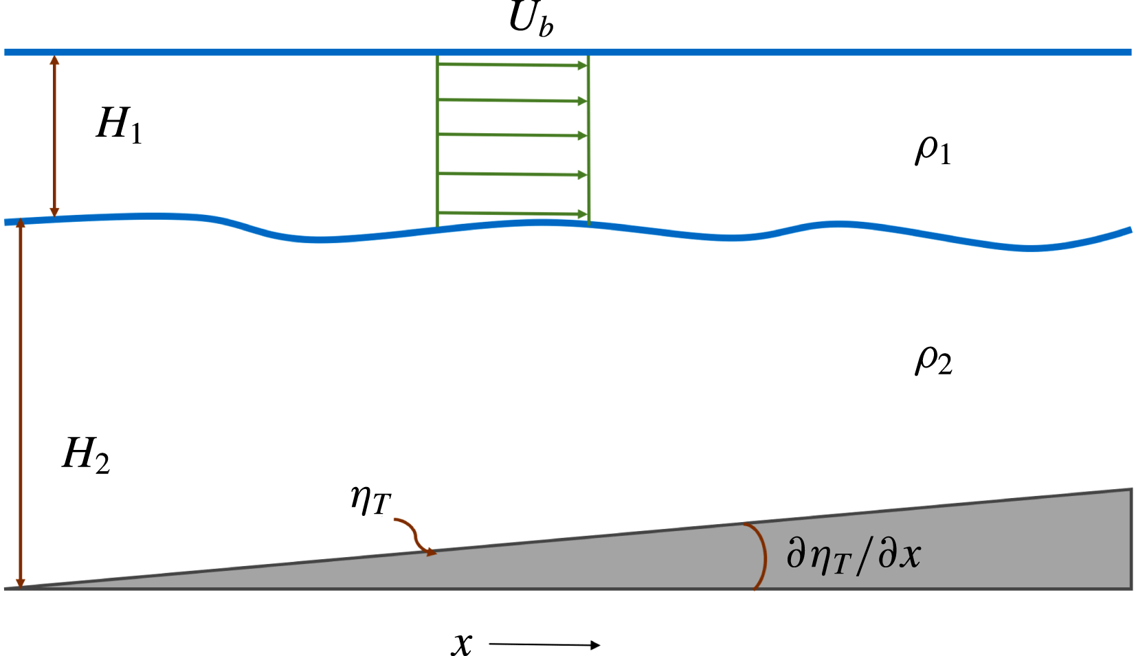
, is used in the study (a sketch of the domain is shown in figure 1). The governing equations in the presence of bottom topography are (Vallis Reference Vallis2017):
 $$\begin{eqnarray}\displaystyle & \displaystyle \frac{\text{D}_{1}}{\text{D}t}[\unicode[STIX]{x1D6FB}^{2}\unicode[STIX]{x1D713}_{1}+S_{1}(\unicode[STIX]{x1D713}_{2}-\unicode[STIX]{x1D713}_{1}+U_{b}y)]+\unicode[STIX]{x1D6FD}\frac{\unicode[STIX]{x2202}\unicode[STIX]{x1D713}_{1}}{\unicode[STIX]{x2202}x}=\unicode[STIX]{x1D708}\unicode[STIX]{x1D6FB}^{4}\unicode[STIX]{x1D713}_{1}, & \displaystyle\end{eqnarray}$$
 $$\begin{eqnarray}\displaystyle & & \displaystyle \displaystyle \frac{\text{D}_{2}}{\text{D}t}[\unicode[STIX]{x1D6FB}^{2}\unicode[STIX]{x1D713}_{2}+S_{2}(\unicode[STIX]{x1D713}_{1}-U_{b}y-\unicode[STIX]{x1D713}_{2})]\nonumber\\ \displaystyle & & \displaystyle \quad +\left(\unicode[STIX]{x1D6FD}+\frac{f_{o}}{H_{2}}\frac{\unicode[STIX]{x2202}\unicode[STIX]{x1D702}_{T}}{\unicode[STIX]{x2202}y}\right)\frac{\unicode[STIX]{x2202}\unicode[STIX]{x1D713}_{2}}{\unicode[STIX]{x2202}x}-\frac{f_{o}}{H_{2}}\frac{\unicode[STIX]{x2202}\unicode[STIX]{x1D702}_{T}}{\unicode[STIX]{x2202}x}\frac{\unicode[STIX]{x2202}\unicode[STIX]{x1D713}_{2}}{\unicode[STIX]{x2202}y}=\unicode[STIX]{x1D708}\unicode[STIX]{x1D6FB}^{4}\unicode[STIX]{x1D713}_{2}-\unicode[STIX]{x1D6FE}\unicode[STIX]{x1D6FB}^{2}\unicode[STIX]{x1D713}_{2},\end{eqnarray}$$
where
 $i=1,2$
indicate the top and bottom isopycnal layers, respectively;
 $\unicode[STIX]{x1D713}_{i}$
is the layer-wise velocity streamfunction;
 $\unicode[STIX]{x1D6FD}$
is the meridional gradient of the Coriolis parameter
 $f=f_{o}+\unicode[STIX]{x1D6FD}y$
(
 $f_{o}$
is the angular velocity due to the Earth’s rotation at some reference latitude);
 $H_{i}$
is the layer thickness;
 $\unicode[STIX]{x1D702}_{T}$
is the bottom topography;
 $S_{i}=f_{o}^{2}/g^{\prime }H_{i}$
(with
 $g^{\prime }=g(\unicode[STIX]{x1D70C}_{2}-\unicode[STIX]{x1D70C}_{1})/\unicode[STIX]{x1D70C}_{1}$
,
 $g$
the gravity acceleration and
 $\unicode[STIX]{x1D70C}_{i}$
the layer density) is the stratification parameter in each layer; and
 $\unicode[STIX]{x1D708}$
,
 $\unicode[STIX]{x1D6FE}$
are eddy viscosity and bottom friction parameters, respectively. Note that
 $$\begin{eqnarray}\frac{\text{D}_{i}}{\text{D}t}=\frac{\unicode[STIX]{x2202}}{\unicode[STIX]{x2202}t}-\frac{\unicode[STIX]{x2202}}{\unicode[STIX]{x2202}y}(\unicode[STIX]{x1D713}_{i}-\unicode[STIX]{x1D6FF}_{i1}U_{b}y)\frac{\unicode[STIX]{x2202}}{\unicode[STIX]{x2202}x}+\frac{\unicode[STIX]{x2202}}{\unicode[STIX]{x2202}x}(\unicode[STIX]{x1D713}_{i}-\unicode[STIX]{x1D6FF}_{i1}U_{b}y)\frac{\unicode[STIX]{x2202}}{\unicode[STIX]{x2202}y},\end{eqnarray}$$
where
 $\unicode[STIX]{x1D6FF}_{ij}=1$
if
 $i=j$
, else
 $\unicode[STIX]{x1D6FF}_{ij}=0$
.
Sketch of the model domain. The upper layer has an imposed uniform eastward background flow
 $U_{b}$
;
 $H_{i}$
and
 $\unicode[STIX]{x1D70C}_{i}$
are the layer depth and layer density in each layer, respectively; and
 $\unicode[STIX]{x1D702}_{T}$
is the bottom topography. Axis
 $y$
points into the sketch.

2.1 Model parameters and spin-up
The computations were performed on a doubly periodic rectangular domain having uniform spatial resolution of
 $512\times 256$
grid points, with the domain length
 $L_{x}$
kept twice the width
 $L_{y}$
(
 $L_{x}=3600$
km;
 $x$
and
 $y$
are the zonal and meridional coordinates, respectively). Most of the parameter values are adapted from Berloff et al. (Reference Berloff, Kamenkovich and Pedlosky2009b
), i.e.
 $\unicode[STIX]{x1D6FD}=2\times 10^{-11}~\text{m}^{-1}~\text{s}^{-1}$
,
 $H_{1}=1$
km,
 $H_{2}=3$
km,
 $S_{1}=1.2\times 10^{-9}~\text{m}^{-2}$
and
 $S_{2}=0.4\times 10^{-9}~\text{m}^{-2}$
. The value of
 $\unicode[STIX]{x1D6FD}$
is at
 $30^{\circ }$
latitude, and the stratification parameters correspond to a baroclinic deformation radius of 25 km, which is typical in the mid-latitudinal ocean (Chelton et al.
Reference Chelton, Deszoeke, Schlax, El Naggar and Siwertz1998). We chose background flow
 $U_{b}$
equal to
 $0.06~\text{m}~\text{s}^{-1}$
, which is a baroclinically unstable flow for the chosen parameter values. Values
 $\unicode[STIX]{x1D708}=100~\text{m}^{2}~\text{s}^{-1}$
and
 $\unicode[STIX]{x1D6FE}=2\times 10^{-8}~\text{s}^{-1}$
were used to remove excess energy from the system. The bottom drag coefficient value has been kept quite small, so that the developed jets are strong and clear – the effects of bottom friction are discussed in Berloff et al. (Reference Berloff, Karabasov, Farrar and Kamenkovich2011).
In this work, we analyse the impacts of a slowly varying topography such that
 $(f_{o}/H_{2})|\unicode[STIX]{x1D735}\unicode[STIX]{x1D702}_{T}|$
is smaller than
 $\unicode[STIX]{x1D6FD}$
; hence, the
 $\unicode[STIX]{x1D6FD}$
-effect controls the jet formation. The idea is to understand the effects of bottom topography on jets that are primarily formed by the
 $\unicode[STIX]{x1D6FD}$
-effect, and not to modify the baroclinic instability process. The dynamics over a very steep topography would also be very interesting to study, but we do not address that in this paper. Here, we concentrate only on the effects of the zonal asymmetry, as a meridional gradient in
 $\unicode[STIX]{x1D702}_{T}$
would be equivalent to an additional
 $\unicode[STIX]{x1D6FD}$
-effect in the deep layer (from (2.2)). Given that
 $\unicode[STIX]{x1D6FD}$
controls the jet formation, a small meridional slope is unlikely to change the dynamics significantly. In fact, we ran a test simulation with a small meridional slope, and compared the flow patterns with a flat bottom simulation. The jets were stationary in both cases, and we observed a negligible difference in the flow patterns. In this work, we consider a topography that increases linearly in the zonal direction. We consider three different cases for
 $T_{x}=(f_{o}/H_{2})(\unicode[STIX]{x2202}\unicode[STIX]{x1D702}_{T}/\unicode[STIX]{x2202}x)$
:
 $8.3\times 10^{-13}$
,
 $1.4\times 10^{-12}$
and
 $2.8\times 10^{-12}~\text{m}^{-1}~\text{s}^{-1}$
. Note that
 $T_{x}$
is still quite small in comparison to
 $\unicode[STIX]{x1D6FD}$
, and the change in depth is also small compared to the thickness of the lower layer. Here we refer to these as ‘small slope’, ‘medium slope’ and ‘large slope’, respectively.
In the numerical simulations, (2.1) and (2.2) were discretised using a second-order finite-difference method and solved with an advanced numerical scheme called CABARET (Karabasov, Berloff & Goloviznin Reference Karabasov, Berloff and Goloviznin2009). The simulations were initialised from a perturbed background state and run for 20 000 days. The system quickly develops mesoscale eddies which then transfer energy upscale to form alternating jets. The jets were largely formed by the simulation time of 1000 days, and it took approximately 4000 days more to reach a statistically steady state, with completely matured jets.
3 Results
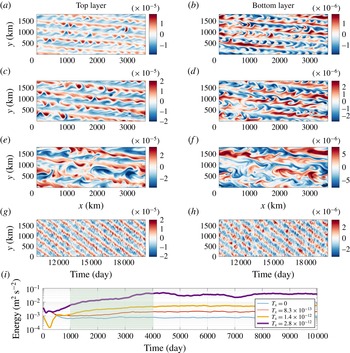
At first, we study the behaviour of alternating jets in the equilibrium state, in which time-mean energy supplied to the system by the background flow is equal to the energy removed by viscous dissipation and bottom drag. Snapshots of the PV anomaly field in the top layer (
 $\unicode[STIX]{x1D6FB}^{2}\unicode[STIX]{x1D713}_{1}+S_{1}(\unicode[STIX]{x1D713}_{2}-\unicode[STIX]{x1D713}_{1})$
) and bottom layer (
 $\unicode[STIX]{x1D6FB}^{2}\unicode[STIX]{x1D713}_{2}+S_{2}(\unicode[STIX]{x1D713}_{1}-\unicode[STIX]{x1D713}_{2})$
) are shown in figure 2(a–f). Alternating jets are tilted from the zonal direction, and the angle increases with the bottom slope (tilt angles are
 $5.71^{\circ }$
,
 $7.13^{\circ }$
and
 $9.46^{\circ }$
in the corresponding reference solutions). Here, the direction of the background PV gradient in the bottom layer (
 $\unicode[STIX]{x1D735}[f_{o}+(\unicode[STIX]{x1D6FD}-S_{2}U_{b})y+T_{x}x]$
) is no longer meridional due to the presence of the zonal asymmetry, and makes a certain angle with the top-layer background PV gradient (
 $\unicode[STIX]{x1D735}[f_{o}+(\unicode[STIX]{x1D6FD}+S_{1}U_{b})y]$
). This affects the direction of Rossby wave propagation and results in the tilted jets. The angle of tilt can be easily estimated in a barotropic model as
 $\tan ^{-1}(T_{x}/\unicode[STIX]{x1D6FD})$
(Boland et al.
Reference Boland, Thompson, Shuckburgh and Haynes2012). However, the dynamics is more complex in multilayer models, where the tilt angle is determined by the combined dynamics of both layers. In the two-layer QG model experiments, Boland et al. (Reference Boland, Thompson, Shuckburgh and Haynes2012) observed that the jets tend to be aligned with the mean barotropic background PV isolines, but there were deviations. In our simulations, the jet tilt angles are always larger than the ones estimated analytically from the barotropic background PV (
 $\unicode[STIX]{x1D703}=\tan ^{-1}[H_{2}T_{x}/((H_{1}+H_{2})\unicode[STIX]{x1D6FD})]$
), which are
 $1.78^{\circ }$
,
 $3.01^{\circ }$
and
 $5.99^{\circ }$
for the chosen slopes. Also, the periodic boundary conditions restrict the jets to tilt at specific angles, because in order to satisfy the boundary conditions, the number of jet pairs has to be an integer, and also the jets have to be evenly spaced. Note that the spatial structure of the PV anomaly field is quite different in the bottom layer in comparison to the top layer. As mentioned above, the mean PV isolines in the layers are no longer parallel; on the other hand, the jets are parallel in both layers. As a result of this, the jets actually cross the mean PV isolines in the bottom layer, which leads to the differences in the PV spatial structure.
General flow patterns and equilibration of the jets. (a–f) Snapshots of the PV anomaly (colour bar units are in
 $\text{s}^{-1}$
) field in the top layer (
 $\unicode[STIX]{x1D735}^{2}\unicode[STIX]{x1D713}_{1}+S_{1}(\unicode[STIX]{x1D713}_{2}-\unicode[STIX]{x1D713}_{1})$
) and bottom layer (
 $\unicode[STIX]{x1D735}^{2}\unicode[STIX]{x1D713}_{2}+S_{2}(\unicode[STIX]{x1D713}_{1}-\unicode[STIX]{x1D713}_{2})$
) from three reference solutions (values of
 $T_{x}$
are given in § 2.1). (g,h) Hovmöller diagram of the PV anomaly field in the top and bottom layers (PV along a cross-section at the centre of the domain is plotted against time for the medium-slope simulation). (i) Total energy time series for different values of
 $T_{x}$
(energy time series for a flat bottom case
 $T_{x}=0$
is shown for reference). The jets tilt at angles
 $5.71^{\circ }$
,
 $7.13^{\circ }$
and
 $9.46^{\circ }$
and drift southwards with speeds 0.20, 0.48 and
 $0.74~\text{cm}~\text{s}^{-1}$
, respectively.

In addition to tilting, the jets drift in the direction perpendicular to their phase lines (see Hovmöller diagram in figure 2
g,h). For positive values of
 $T_{x}$
, the jets drift to the south (the opposite is true for negative values of
 $T_{x}$
). The drift speed remains nearly constant with time, as the pathlines created with jet positions at different times are almost straight. Similar to the tilt angle, the drift speed also increases with the bottom slope. In the reference solutions, the drift speeds are approximately 0.20, 0.48 and
 $0.74~\text{cm}~\text{s}^{-1}$
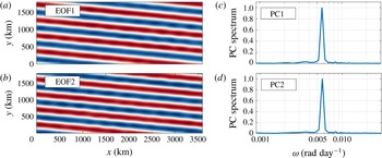
, respectively. In order to compute the exact jet drift velocities in the reference solutions, we applied the principal component (PC) analysis (Hannachi, Jolliffe & Stephenson Reference Hannachi, Jolliffe and Stephenson2007) to the full flow and decomposed the velocity streamfunction field into a set of spatially coherent and temporally uncorrelated patterns. The first two empirical orthogonal functions (EOFs) are in quadrature and capture the drifting jets. The power spectra of the corresponding PCs have narrow peaks at the single frequency corresponding to the drift velocity (figure 3). The peak frequency
 $\unicode[STIX]{x1D714}$
and the wavevector
 $\boldsymbol{k}=(2\unicode[STIX]{x03C0}/L_{x})\hat{\boldsymbol{i}}+(2\unicode[STIX]{x03C0}n/L_{y})\hat{\boldsymbol{j}}$
(
 $n$
is the number of jet pairs in the simulations, and
 $\hat{\boldsymbol{i}}$
and
 $\hat{\boldsymbol{j}}$
are the zonal and meridional unit vectors, respectively) corresponding to the jets are then used to compute the drift velocity
 $\boldsymbol{c}=(\unicode[STIX]{x1D714}/|\boldsymbol{k}|)\boldsymbol{k}$
. We also verified that the tilt angles and drift speeds are independent of the numerical model resolution and domain size.
Principal component analysis of the streamfunction field from the medium-slope simulation: (a,b) EOF 1, 2 in the top layer (colour bar range is
 $[-1,~1]$
); (c,d) power spectra of PCs (normalised to unity) corresponding to the first two EOFs. Drifting jets are analogous to a propagating wave, and two EOFs, which are identical but with a phase shift of
 $\unicode[STIX]{x03C0}/2$
, are sufficient to represent the wave. PCs corresponding to these EOFs continuously oscillate between the maximum and minimum values to reflect the propagation of the jets; thus, their power spectra show peaks at a definite frequency. Since the wavevector
 $\boldsymbol{k}$
and peak frequency
 $\unicode[STIX]{x1D714}$
corresponding to the EOFs are known, the drift velocity of the jets can be computed as
 $\boldsymbol{c}=(\unicode[STIX]{x1D714}/|\boldsymbol{k}|)\boldsymbol{k}$
.

Even though the jets are well formed by 1000 days, the total energy of the system continuously increases until approximately 4000 days, when it reaches a statistical equilibrium. The total equilibrated flow energy
 $(1/2A)\int _{A}[H_{1}|\unicode[STIX]{x1D735}\unicode[STIX]{x1D713}_{1}|^{2}+H_{2}|\unicode[STIX]{x1D735}\unicode[STIX]{x1D713}_{2}|^{2}+H_{1}S_{1}(\unicode[STIX]{x1D713}_{1}-\unicode[STIX]{x1D713}_{2})^{2}]$
(where
 $A$
is the area of the domain, and note that
 $H_{1}S_{1}=H_{2}S_{2}$
) increases with zonal slope (figure 2
i). We also found tilted, drifting jets in numerical simulations in a channel configuration, where partial-slip boundary conditions were imposed on the northern and southern boundaries. The details are given in appendix A. The presence of boundaries makes the dynamics more complex, as secondary circulations are created along the boundaries. However, we do not focus on those effects in this work and restrict ourselves to periodic domains.
We observed only three to five pairs of jets for the choice of parameter values. This is problematic in the sense that there are limited tilt angles allowed by the periodic boundaries. Given this, the tilt angles in the simulations may have been overestimated, which would then affect the drift speeds. This effect can be minimised by using a very large domain, which would increase the number of jet pairs in the system. However, that would be computationally too expensive to simulate. Nevertheless, the choice of a periodic domain does not affect the final conclusion of the paper, as our aim here is only to study the drift mechanism, and not to associate tilt angles and drift speeds with topographic slope magnitudes.
3.1 Drift velocities from the linear dispersion relation
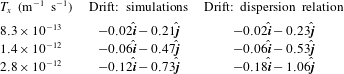
Although the jet tilting is associated with the tilting of barotropic PV isolines, it is not clear why the jets drift in the presence of a zonal component of PV gradient. In order to address this aspect, we analysed the dispersion relation derived from the two-layer QG model (from (2.1) and (2.2), see appendix B for details) and found frequencies (real parts of the eigenvalues) for eigenmodes matching the jets in the reference solutions. The eigenmodes possess non-zero frequencies, which means that they propagate. The corresponding phase velocities are then compared with the drift velocities estimated from the reference solutions (table 1). The predictions from the dispersion relation are quite close to the fully nonlinear solutions, although the nonlinearities seem to slow the jets down, as the observed drift speeds are slightly smaller than the linear predictions. The difference increases with zonal slope and is almost 30 % in the large-slope simulation. On the basis of these comparisons, we conclude that the linear dispersion relation can be used to predict jet drift speeds, at least for mild zonal slopes. However, the prediction from the linear dispersion relation does not work very well in cases where
 $O(T_{x})\rightarrow O(\unicode[STIX]{x1D6FD})$
. This comparison is possible because linear dynamics governs a major part of the flow, and the jets correspond to the eigenmodes, which are solutions of the linear problem (Berloff & Kamenkovich Reference Berloff and Kamenkovich2013a
,Reference Berloff and Kamenkovich
b
). The main difference is that, unlike zonal eigenmodes over a flat bottom, tilted eigenmodes are not steady but propagate with constant velocities. As we show in the next section, eddies also contribute to the drift by slowing the jets down.
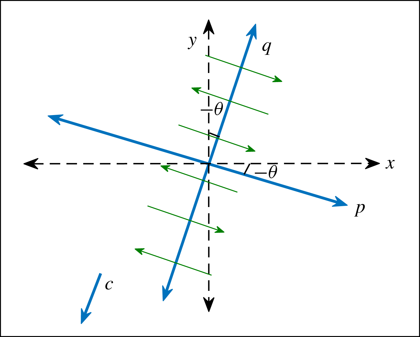
Sketch of the new coordinate system (new axes are
 $p$
and
 $q$
) that is rotated by an angle
 $\unicode[STIX]{x1D703}$
(tilt is positive for anticlockwise rotation) and is moving with a speed
 $c$
(drift speed, positive in
 $q$
direction). Angle
 $\unicode[STIX]{x1D703}$
and speed
 $c$
are directly estimated from the numerical solutions. Green arrows represent the alternating jets; note that the time-mean profile of the jets is a function of
 $q$
only.

Comparison of drift velocities (
 $\text{cm}~\text{s}^{-1}$
) in the numerical simulations and dispersion relation. Overall, the comparison is good but there is a systematic difference for steeper slopes.
 $\hat{\boldsymbol{i}}$
and
 $\hat{\boldsymbol{j}}$
are the zonal and meridional unit vectors, respectively.

3.2 Nonlinear effects and the role of eddies
In the case of purely zonal and stationary jets, the flow can be Reynolds-style decomposed into the time-mean large-scale flow and transient eddies, and the time-mean (or zonally averaged) meridional profiles of nonlinear eddy stress terms can be analysed (e.g. Panetta Reference Panetta1993; Berloff et al.
Reference Berloff, Kamenkovich and Pedlosky2009a
). Through a continuous baroclinic instability process, the eddies gain energy from the available potential energy of the system and interact with the jets via exchanges of momentum and PV, and one can study this process by comparing and correlating cross-jet profiles of the eddy forcing and time-mean PV. However, in the case of drifting jets, the analysis is not that straightforward, as the mean state itself is time-dependent. To overcome this problem, we used a new frame of reference in which the jets are stationary and aligned with one of the coordinates. In the new configuration, shown in figure 4, the frame of reference is rotated by the jet tilt angle
 $\unicode[STIX]{x1D703}$
and moves with a constant speed
 $c$
(equal to the jet drift speed). Note that PV conservation holds true irrespective of the frame of reference, as long as there is no additional acceleration. Thus, the governing equations (2.1) and (2.2) can be rewritten in the new frame of reference and interpreted as PV conservation laws (note that
 $\unicode[STIX]{x1D713}_{i}=\unicode[STIX]{x1D713}_{i}(p,q,t)$
):
 $$\begin{eqnarray}\displaystyle & \displaystyle \left[\frac{\unicode[STIX]{x2202}}{\unicode[STIX]{x2202}t}-c\frac{\unicode[STIX]{x2202}}{\unicode[STIX]{x2202}q}\right]\unicode[STIX]{x1D6F1}_{1}=-\left(\frac{\unicode[STIX]{x2202}\unicode[STIX]{x1D713}_{1}}{\unicode[STIX]{x2202}p}-U_{b}\sin \unicode[STIX]{x1D703}\right)\frac{\unicode[STIX]{x2202}\unicode[STIX]{x1D6F1}_{1}}{\unicode[STIX]{x2202}q}+\left(\frac{\unicode[STIX]{x2202}\unicode[STIX]{x1D713}_{1}}{\unicode[STIX]{x2202}q}-U_{b}\cos \unicode[STIX]{x1D703}\right)\frac{\unicode[STIX]{x2202}\unicode[STIX]{x1D6F1}_{1}}{\unicode[STIX]{x2202}p}+\unicode[STIX]{x1D708}\unicode[STIX]{x1D6FB}^{4}\unicode[STIX]{x1D713}_{1}, & \displaystyle \nonumber\\ \displaystyle & & \displaystyle\end{eqnarray}$$
 $$\begin{eqnarray}\displaystyle & \displaystyle \left[\frac{\unicode[STIX]{x2202}}{\unicode[STIX]{x2202}t}-c\frac{\unicode[STIX]{x2202}}{\unicode[STIX]{x2202}q}\right]\unicode[STIX]{x1D6F1}_{2}=-\frac{\unicode[STIX]{x2202}\unicode[STIX]{x1D713}_{2}}{\unicode[STIX]{x2202}p}\frac{\unicode[STIX]{x2202}\unicode[STIX]{x1D6F1}_{2}}{\unicode[STIX]{x2202}q}+\frac{\unicode[STIX]{x2202}\unicode[STIX]{x1D713}_{2}}{\unicode[STIX]{x2202}q}\frac{\unicode[STIX]{x2202}\unicode[STIX]{x1D6F1}_{2}}{\unicode[STIX]{x2202}p}+\unicode[STIX]{x1D708}\unicode[STIX]{x1D6FB}^{4}\unicode[STIX]{x1D713}_{2}-\unicode[STIX]{x1D6FE}\unicode[STIX]{x1D6FB}^{2}\unicode[STIX]{x1D713}_{2}, & \displaystyle\end{eqnarray}$$
where
 $$\begin{eqnarray}\left.\begin{array}{@{}l@{}}\displaystyle \unicode[STIX]{x1D6F1}_{1}=\overbrace{\unicode[STIX]{x1D6FB}^{2}\unicode[STIX]{x1D713}_{1}+S_{1}(\unicode[STIX]{x1D713}_{2}-\unicode[STIX]{x1D713}_{1})}^{Q_{1}}+\,(\unicode[STIX]{x1D6FD}+S_{1}U_{b})(q\cos \unicode[STIX]{x1D703}+p\sin \unicode[STIX]{x1D703}+ct\cos \unicode[STIX]{x1D703}),\\ \displaystyle \unicode[STIX]{x1D6F1}_{2}=\overbrace{\unicode[STIX]{x1D6FB}^{2}\unicode[STIX]{x1D713}_{2}+S_{2}(\unicode[STIX]{x1D713}_{1}-\unicode[STIX]{x1D713}_{2})}^{Q_{2}}+\,(\unicode[STIX]{x1D6FD}-S_{2}U_{b})(q\cos \unicode[STIX]{x1D703}+p\sin \unicode[STIX]{x1D703}+ct\cos \unicode[STIX]{x1D703})\\ \qquad +\,T_{x}(-q\sin \unicode[STIX]{x1D703}+p\cos \unicode[STIX]{x1D703}-ct\sin \unicode[STIX]{x1D703}).\end{array}\right\}\end{eqnarray}$$
Here,
 $\unicode[STIX]{x1D6F1}_{i}$
represents the absolute PV (i.e. the sum of PV due to the generated flow
 $Q_{i}$
and the background PV) in individual layers. Also note that all variables are functions of
 $p,~q,~t$
and
 $\unicode[STIX]{x1D735}=(\unicode[STIX]{x2202}/\unicode[STIX]{x2202}p,\unicode[STIX]{x2202}/\unicode[STIX]{x2202}q)$
. The first two terms on the right-hand side of (3.1) and (3.2) contain both linear and nonlinear terms, which are due to the background PV gradients, generated flow and nonlinear eddy effects. Depending on the overall sign of the sum,
 $Q_{i}$
can be forced or damped, resulting in strengthening or weakening of the jets. The rest of the terms on the right-hand side always smooth the PV gradients by removing energy from the system through viscous dissipation and bottom drag. In order to understand the effects of eddies and linear terms, we derived the time-mean equations from (3.1) and (3.2) by representing the variables as a sum of the time-mean flow (
 $\overline{Q}_{i}$
,
 $\overline{\unicode[STIX]{x1D713}}_{i}$
) and time-dependent eddy field (
 $Q_{i}^{\prime }$
,
 $\unicode[STIX]{x1D713}_{i}^{\prime }$
). This is basically the Reynolds flow decomposition in the moving frame of reference. The equations are then averaged over time (see full derivation in appendix C):
 $$\begin{eqnarray}\displaystyle & \displaystyle \frac{\unicode[STIX]{x2202}\overline{Q}_{1}}{\unicode[STIX]{x2202}t}=\underbrace{-\unicode[STIX]{x1D735}\boldsymbol{\cdot }\overline{(\boldsymbol{u}_{1}^{\prime }Q_{1}^{\prime })}}_{\text{eddy forcing}}+\underbrace{\overbrace{(c+U_{b}\sin \unicode[STIX]{x1D703})\frac{\unicode[STIX]{x2202}\overline{Q}_{1}}{\unicode[STIX]{x2202}q}}^{L_{1}^{c}}\overbrace{-\,(\unicode[STIX]{x1D6FD}+S_{1}U_{b})\sin \unicode[STIX]{x1D703}\,\,\overline{u}_{1}}^{L_{1}^{m}}}_{\text{linear stress terms}}+\underbrace{\overbrace{\unicode[STIX]{x1D708}\unicode[STIX]{x1D6FB}^{2}\overline{\unicode[STIX]{x1D701}}_{1}}^{D_{1}^{\unicode[STIX]{x1D708}}}}_{\text{dissipation}},\qquad & \displaystyle\end{eqnarray}$$
 $$\begin{eqnarray}\displaystyle & \displaystyle \frac{\unicode[STIX]{x2202}\overline{Q}_{2}}{\unicode[STIX]{x2202}t}=\overbrace{-\unicode[STIX]{x1D735}\boldsymbol{\cdot }\overline{(\boldsymbol{u}_{2}^{\prime }Q_{2}^{\prime })}}^{\text{eddy forcing}}+\overbrace{\underbrace{c\frac{\unicode[STIX]{x2202}\overline{Q}_{2}}{\unicode[STIX]{x2202}q}}_{L_{2}^{c}}\underbrace{-\,[(\unicode[STIX]{x1D6FD}-S_{2}U_{b})\sin \unicode[STIX]{x1D703}+T_{x}\cos \unicode[STIX]{x1D703}]\,\overline{u}_{2}}_{L_{2}^{m}}}^{\text{linear stress terms}}+\overbrace{\underbrace{\unicode[STIX]{x1D708}\unicode[STIX]{x1D6FB}^{2}\overline{\unicode[STIX]{x1D701}}_{2}}_{D_{2}^{\unicode[STIX]{x1D708}}}\underbrace{-\,\unicode[STIX]{x1D6FE}\overline{\unicode[STIX]{x1D701}}_{2}}_{D_{2}^{\unicode[STIX]{x1D6FE}}}}^{\text{dissipation}},\qquad & \displaystyle\end{eqnarray}$$
where
 $\boldsymbol{u}_{i}$
is the new velocity (
 $\boldsymbol{u}_{i}=(u_{i},v_{i})=(-\unicode[STIX]{x2202}\unicode[STIX]{x1D713}_{i}/\unicode[STIX]{x2202}q,\unicode[STIX]{x2202}\unicode[STIX]{x1D713}_{i}/\unicode[STIX]{x2202}p)$
) and
 $\unicode[STIX]{x1D701}_{i}$
is the new relative vorticity (
 $\unicode[STIX]{x1D701}_{i}=\unicode[STIX]{x1D6FB}^{2}\unicode[STIX]{x1D713}_{i}$
) in each layer. Here, we retain the time derivatives in the time-mean PV (in the rest of the paper, ‘mean PV’ refers to the mean PV of the developed flow only i.e.
 $\overline{Q}_{i}$
), but the terms vanish in the steady state and are kept here only for clarity. As seen in (3.4) and (3.5), the nonlinear terms (referred to hereafter as ‘eddy forcing’ or ‘nonlinear stress term’) and the linear terms (‘linear stress terms’
 $L_{i}^{c}+L_{i}^{m}$
, and ‘dissipation terms’
 $D_{i}^{\unicode[STIX]{x1D708}}+D_{i}^{\unicode[STIX]{x1D6FE}}$
) balance each other in the stationary equilibrated state.
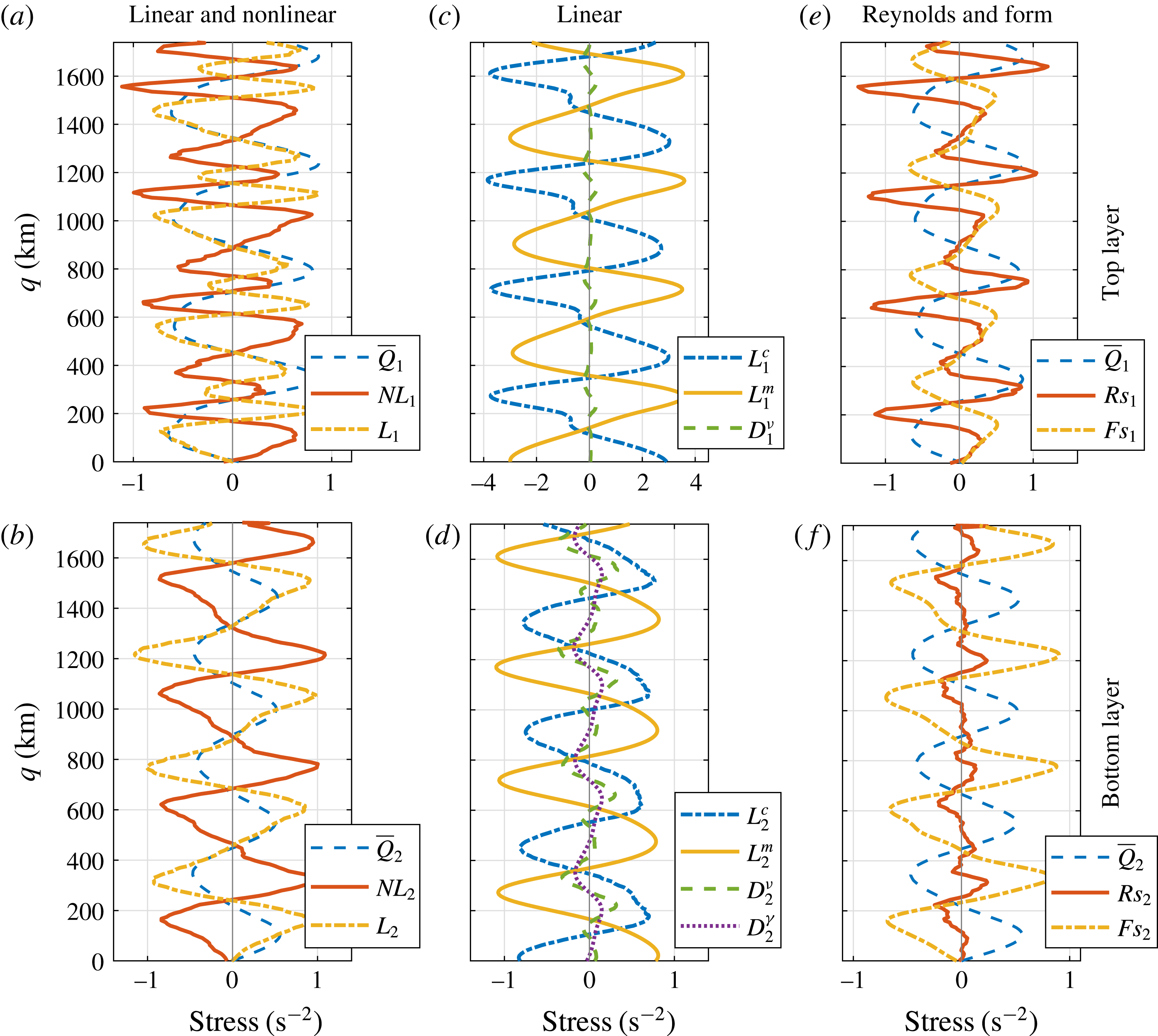
Cross-jet profiles for the medium-slope simulation averaged in the moving frame in the interval 10 000–20 000 days. (a,b) Eddy forcing (
 $NL_{i}$
, smoothed with 10-point moving average) and linear stress terms plus dissipation terms (
 $L_{i}$
). (c,d) Radiation stress term, inertial stress term and dissipation terms. (e,f) Reynolds stress term and form stress term (smoothed with 10-point moving average). Top and bottom rows are for the top and bottom layers, respectively. In order to normalise the plots, the stress terms (units are in
 $\text{s}^{-2}$
) are multiplied by factors of
 $5\times 10^{12}$
and
 $2\times 10^{13}$
in the top and bottom layers, respectively. Dashed blue curves in (a,b,e,f) represent the time-mean PV profiles (
 $\overline{Q}_{i}$
, normalised), which are multiplied by factors of
 $2.2\times 10^{5}$
and
 $8.8\times 10^{5}$
in the top and bottom layers, respectively. The eddies act against the jets, whereas the jets are forced by the linear stress terms.

In order to compute the eddy forcing and linear stress terms, we first linearly interpolated the streamfunction field on a rectangular grid rotated by the jet tilt angle
 $\unicode[STIX]{x1D703}$
and aligned the streamfunction snapshots in the moving frame of reference at every time step. We then computed the stress terms using the relations (3.4) and (3.5) and averaged them over time and along the jets. Cross-jet profiles of these linear and nonlinear stress terms for the medium-slope solution are shown in figure 5. As expected from the equations, the linear and nonlinear stress terms balance each other (figure 5
a,b). (There are small deviations from zero due to the data interpolation. An interpolation scheme with higher-order accuracy could be used, but we found linear interpolation to be sufficient for our purposes. In fact, we also computed the stress terms in the original
 $xy$
coordinate system and interpolated the stress field, but the resulting differences were found to be insignificant.) Relative contributions of the individual linear terms are also analysed (see figure 5
c,d): the
 $L^{c}$
and
 $L^{m}$
terms (hereafter referred to as ‘radiation stress term’ and ‘inertial stress term’, respectively) in the top layer are almost four times larger in magnitude than the eddy forcing, whereas all these terms are of comparable strength in the bottom layer. In the top layer, the radiation and inertial stress terms largely balance each other, and the difference between them is compensated by the eddy forcing. In both layers, the dissipation terms are significantly small and can be safely neglected. In terms of kinetic energy, the top layer dominates over the bottom layer and is two to three times more energetic (not shown). Thus, this supports the hypothesis that linear modes control a major part of the flow dynamics and hence the drift.
Correlation coefficients between cross-jet profiles of the time-mean linear and nonlinear stress terms, and the time-mean PV (
 $\overline{Q}_{i}$
) in both layers for the medium-slope simulation. The linear stress terms support the jets, whereas the eddy forcing opposes them.

It is important to note that the eddy forcing tends to smooth the mean PV profile in both layers and counteract the linear stress terms (figure 5
a,b). We computed correlation coefficients between the cross-jet profiles of the time-mean PV and stress terms. The linear stress terms are positively correlated (correlation coefficients
 ${\sim}0.6$
) with the time-mean PV, whereas the eddy forcing terms show negative correlation (
 ${\sim}-0.3$
) with the time-mean PV (table 2). This is in contrast to previous studies on oceanic jets (Berloff et al.
Reference Berloff, Kamenkovich and Pedlosky2009a
,Reference Berloff, Kamenkovich and Pedlosky
b
; Chen et al.
Reference Chen, Kamenkovich and Berloff2015) and jets in planetary atmospheres (Ingersoll et al.
Reference Ingersoll, Beebe, Mitchell, Garneau, Yagi and Müller1981; Panetta Reference Panetta1993; Ingersoll et al.
Reference Ingersoll, Gierasch, Banfield, Vasavada and Team2000), where the jets are essentially eddy-driven. To clarify this matter, we decomposed the eddy forcing into the Reynolds stress term (
 $Rs$
) and form stress term (
 $Fs$
):
 $$\begin{eqnarray}\displaystyle & \displaystyle Rs_{i}=-\unicode[STIX]{x1D735}\boldsymbol{\cdot }\overline{(\boldsymbol{u}_{i}^{\prime }\unicode[STIX]{x1D701}_{i}^{\prime })}, & \displaystyle\end{eqnarray}$$
 $$\begin{eqnarray}\displaystyle & \displaystyle Fs_{i}=-\unicode[STIX]{x1D716}_{i}S_{i}\unicode[STIX]{x1D735}\boldsymbol{\cdot }\overline{(\boldsymbol{u}_{i}^{\prime }(\unicode[STIX]{x1D713}_{2}^{\prime }-\unicode[STIX]{x1D713}_{1}^{\prime }))}, & \displaystyle\end{eqnarray}$$
where
 $\unicode[STIX]{x1D716}_{1}=-\unicode[STIX]{x1D716}_{2}=1$
, and
 $i=1$
, 2 for the top and bottom layers, respectively. Note that the Reynolds stress term and form stress term are simply the convergence of eddy fluxes of relative vorticity and buoyancy, respectively. As shown in figure 5(e,f), the form stress term tends to smooth the PV gradients (correlation coefficients between the form stress term and mean PV profiles are
 ${\sim}-0.9$
in both layers); hence, the form stress term opposes the jets. On the other hand, the Reynolds stress term shows a positive (no) correlation with the mean PV in the top (bottom) layer, which means that only the upper-layer Reynolds stress term forces the jets – see also the discussion in Thompson & Young (Reference Thompson and Young2007). The former observation is comforting in terms of theoretical aspects, because the form stress term is expected to be against the mean PV in a baroclinically unstable flow system forced with an eastward background flow (Berloff et al.
Reference Berloff, Kamenkovich and Pedlosky2009a
). The Reynolds stress term and form stress term are comparable in magnitude in the top layer; however, in the bottom layer, the magnitude of the Reynolds stress term is quite small in comparison to the form stress term, and the effect of the form stress term is more prominent. In the absence of topography, the Reynolds stress term, which is responsible for maintaining the jets in the eastward background shears, dominates over the form stress term and, overall, the eddy forcing is positively correlated with the mean PV. However, here, in the presence of zonal bottom slope, the form stress term overcomes the Reynolds stress term and the overall impact of the eddies is the opposite. This is also in agreement with the linear predictions, which say that any zonal variation in bottom topography enhances the baroclinic instability (Hart Reference Hart1975; Chen & Kamenkovich Reference Chen and Kamenkovich2013). In a study of the North Atlantic jets, Kamenkovich, Berloff & Pedlosky (Reference Kamenkovich, Berloff and Pedlosky2009) also found both kinds of eddy feedbacks (see also Melnichenko et al.
Reference Melnichenko, Maximenko, Schneider and Sasaki2010; Barthel et al.
Reference Barthel, Hogg, Waterman and Keating2017; Youngs et al.
Reference Youngs, Thompson, Lazar and Richards2017). It is important to note that, if the eddy field is computed by high-pass time filtering in a stationary frame of reference, then the resulting eddy field would also include the drifting jets. Thus, the eddy forcing would include terms interpreted as linear stress terms in this study. This may complicate comparison between our work and some earlier studies.
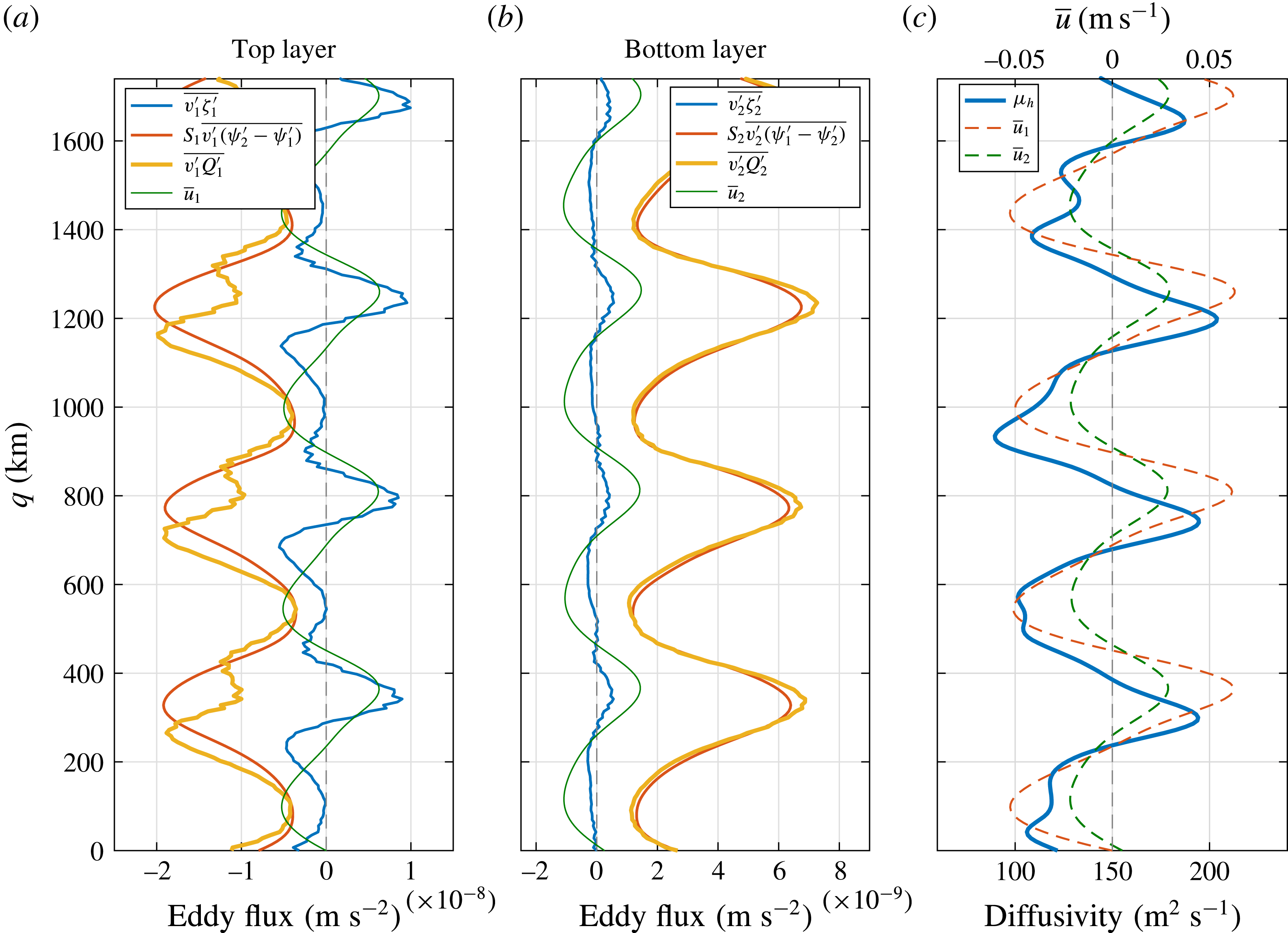
Cross-jet profiles for the medium-slope simulation averaged in the moving frame in the interval 10 000–20 000 days. (a,b) Eddy PV flux
 $\overline{v_{i}^{\prime }Q_{i}^{\prime }}$
, eddy relative vorticity flux
 $\overline{v_{i}^{\prime }\unicode[STIX]{x1D701}_{i}^{\prime }}$
and eddy buoyancy flux
 $\unicode[STIX]{x1D716}_{i}S_{i}\,\overline{v_{i}^{\prime }(\unicode[STIX]{x1D713}_{2}^{\prime }-\unicode[STIX]{x1D713}_{1}^{\prime })}$
across the jets (smoothed with 10-point moving average). (c) Heat diffusivity. The thin green curves in (a,b) represent the mean flow (normalised) in individual layers, and actual magnitudes of the velocities are shown in (c).

We also analysed the cross-jet profiles of the eddy PV fluxes
 $\overline{v_{i}^{\prime }Q_{i}^{\prime }}$
, relative vorticity fluxes
 $\overline{v_{i}^{\prime }\unicode[STIX]{x1D701}_{i}^{\prime }}$
and buoyancy fluxes
 $\unicode[STIX]{x1D716}_{i}S_{i}\,\overline{v_{i}^{\prime }(\unicode[STIX]{x1D713}_{2}^{\prime }-\unicode[STIX]{x1D713}_{1}^{\prime })}$
across the jets (figure 6
a,b). The eddy PV fluxes have most of the contribution from the eddy buoyancy fluxes (also referred to as ‘eddy heat fluxes’), which are uniformly negative (positive) in the top (bottom) layer. In order to understand the role of the eddy buoyancy fluxes, we computed the eddy heat diffusivity
 $\unicode[STIX]{x1D707}_{h}$
,
 $$\begin{eqnarray}\unicode[STIX]{x1D707}_{h}=\frac{\unicode[STIX]{x1D716}_{i}S_{i}\,\overline{v_{i}^{\prime }(\unicode[STIX]{x1D713}_{2}^{\prime }-\unicode[STIX]{x1D713}_{1}^{\prime })}}{-\unicode[STIX]{x2202}_{q}\overline{b}_{i}}=\frac{\unicode[STIX]{x1D716}_{i}S_{i}\,\overline{v_{i}^{\prime }(\unicode[STIX]{x1D713}_{2}^{\prime }-\unicode[STIX]{x1D713}_{1}^{\prime })}}{-\unicode[STIX]{x2202}_{q}(\unicode[STIX]{x1D716}_{i}S_{i}(\overline{\unicode[STIX]{x1D713}}_{2}-\overline{\unicode[STIX]{x1D713}}_{1})+\unicode[STIX]{x1D716}_{i}S_{i}U_{b}q\cos \unicode[STIX]{x1D703})}=\frac{\overline{v_{i}^{\prime }(\unicode[STIX]{x1D713}_{2}^{\prime }-\unicode[STIX]{x1D713}_{1}^{\prime })}}{\overline{u}_{2}-\overline{u}_{1}-U_{b}\cos \unicode[STIX]{x1D703}},\end{eqnarray}$$
where
 $\overline{b}_{i}$
represents the time-mean buoyancy in the layer. Note that the notation is the same as in (3.6) and (3.7). Although the heat diffusivity relations are different in the top and bottom layers, they are mathematically equivalent and would result in the same cross-jet profile of the heat diffusivity in both layers. As shown in figure 6(c), the heat diffusivity is positive everywhere. This means that the eddies advect buoyancy anomaly in the direction of decreasing
 $\overline{b}$
, resulting in the smoothing of mean PV gradients, or, in other words, the eddy buoyancy fluxes are down-gradient. The minima in the eddy heat diffusivity profile coincide with the westward jets, whereas the eddy heat diffusivity is strongest just south of the eastward jets. Since the largest eddy flux covers the eastward jet core, the dynamics is profoundly different from the barotropic ‘PV staircases’ characterised by partial eddy transport barriers located on the eastward jet cores (e.g. Dritschel & McIntyre Reference Dritschel and McIntyre2008). Also, the magnitude of the eddy heat diffusivity increases with zonal slope. On the other hand, the eddy relative vorticity fluxes force the jets (figure 6
a,b), as they are strongly correlated with the mean flow (see expression (15.21) in Vallis Reference Vallis2017). Since eddy heat diffusivity and PV diffusivity are not the same, eddy PV diffusivity was also computed in each layer and the PV diffusivity magnitudes were found to be largely positive. Overall, the eddy buoyancy fluxes dominate over the eddy relative vorticity fluxes; hence, the eddy PV fluxes are down-gradient. The roles of these fluxes are the same, as in the case of stationary zonal jets (Panetta Reference Panetta1993; Thompson & Young Reference Thompson and Young2007), and only the relative magnitudes of the relative vorticity and buoyancy fluxes change because of the zonal asymmetry.
Given this, there must exist a critical value of zonal slope where the effects of the Reynolds stress term and form stress term exactly counter each other, and eddies start to oppose the jets beyond that critical slope. We computed correlation coefficients between the eddy forcing and mean PV profiles in simulations with different zonal slope magnitudes (table 3). Over a flat bottom, jets are supported by the eddy forcing and this is clearly captured by a strong positive correlation in the top layer for
 $T_{x}=0$
. As the zonal slope increases, the eddy forcing correlation coefficient in the top layer changes sign from positive to negative. On the other hand, correlation coefficients in the bottom layer are negative in all cases. This is mostly because only the upper-layer Reynolds stress term is responsible for maintaining the jets (Thompson & Young Reference Thompson and Young2007), whereas the lower-layer Reynolds stress term is small in magnitude and does not have any significant effect (see figure 5
f). It should be noted that the critical slope value computed here is not unique, and it would differ in different parameter regimes. Moreover, periodic boundary conditions may also affect the value of critical slope.
Looking at both the eddy forcing and eddy PV fluxes, we conclude that the vertical structure plays a significant part in deciding the role of eddies. Oceanic eddies are complex, as they can either force or damp a large-scale circulation. The primary role of the eddies is to stabilise the system and bound the alternating jets. In the case of a flat bottom, eddies force the jets and compensate for the energy removed through dissipation. The bounding mechanism is due to over-localisation of the eddies and the resulting loss of the eddy forcing efficiency (Berloff et al.
Reference Berloff, Karabasov, Farrar and Kamenkovich2011). In contrast, in the presence of zonal slope, the jets are no longer parallel to the imposed background flow and can be directly forced by the vertical shear, as seen in the inertial stress term
 $L^{m}$
. Here, the eddies act against the jets to balance the linear forcing, so that the jets can be stabilised and bounded.
Correlation coefficients between the cross-jet profiles of the time-mean nonlinear stress terms, and the time-mean PV (
 $\overline{Q}_{i}$
) in both layers in different simulations (all parameters were kept the same, as given in § 2.1, except
 $T_{x}$
). As the zonal slope is increased, eddies change their behaviour from being jet-supporting to jet-opposing.

3.3 Jet drift mechanism
The analysis in the previous sections predicts that the linear dynamics controls the jet drift. In order to understand this physically, the linear stress terms in expressions (3.4) and (3.5) need to be examined more carefully. Here, the inertial stress term, which is the forcing term for the mean PV, is proportional to the developed mean flow. By construction, the maxima of the mean along-jet velocity and mean PV profiles do not align and are significantly offset. Similarly, the radiation stress term, which partially compensates against the inertial stress term, is also significantly shifted and, in fact, exactly orthogonal to the mean PV profile (i.e. zero correlation), as it is proportional to the first derivative of
 $\overline{Q}_{i}$
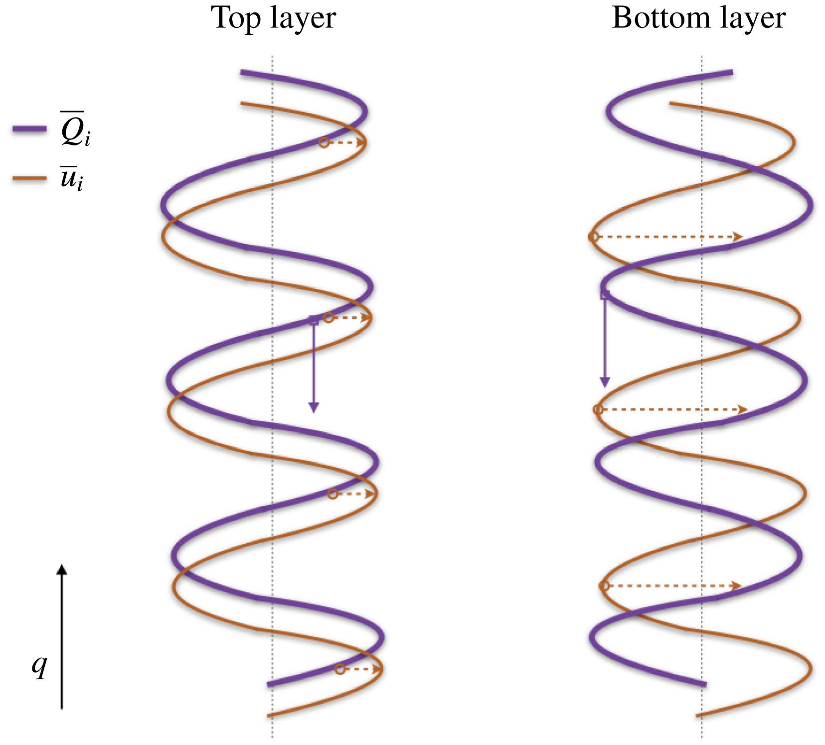
(see table 4 for the maximum/minimum correlation coefficients and corresponding lead/lag phases). In contrast, the eddy forcing maxima are almost aligned with the mean PV maxima, and there is a negligible improvement in correlations with the time-lagged profiles (table 5). The maximum increase in local PV occurs at the locations of the along-jet velocity maxima (figure 7). To account for PV conservation along with this local PV increase, the jets drift southwards. In other words, the off-core linear forcing pushes the jets in the meridional direction. The same is true for northward drifting jets in the case of a negative zonal slope, where the relative shifts between the mean PV and mean flow are simply reversed.
Correlation coefficients and maximum/minimum lag-correlation coefficients between the time-mean cross-jet profiles of the linear stress terms and the time-mean PV (
 $\overline{Q}_{i}$
) in both layers for the medium-slope simulation. Here, the lag period of
 $2\unicode[STIX]{x03C0}$
is equivalent to the meridional width of one pair of jets.

Sketch of cross-jet profiles of the time-mean PV (blue thick) and mean flow (red-brown thin) in both layers in numerical simulations with positive zonal slopes in topography (relative magnitudes are not to scale). The maxima of the mean flow and mean PV profiles do not align, and there is a large shift. Red dashed arrows indicate the tendency of PV to increase/decrease at the velocity maxima due to the mean flow, and blue solid arrows indicate the direction of the drift. Vertical dotted lines represent the zero lines.

Correlation coefficients and maximum/minimum lag-correlation coefficients between the time-mean cross-jet profiles of Reynolds stress term and form stress term, and the time-mean PV (
 $\overline{Q}_{i}$
) in both layers for the medium-slope simulation. Here, the lag period of
 $2\unicode[STIX]{x03C0}$
is equivalent to the meridional width of one pair of jets.

The drift mechanism also agrees with the hypothesis by Boland et al. (Reference Boland, Thompson, Shuckburgh and Haynes2012). They suggest that the jet drift is a result of PV conservation, and the along-jet PV advection is compensated by a meridional drift. From (3.4) and (3.5), it is clear that the inertial stress term is basically advection of a PV component by the mean flow, and the jets drift to compensate for this advection (see expression of the radiation stress term). Melnichenko et al. (Reference Melnichenko, Maximenko, Schneider and Sasaki2010) studied the role of eddy fluxes in the formation of striations in the Pacific. They also showed that linear advection terms appear in the time-averaged PV budget due to the non-zero angle between the background flow and tilted striations. Here, too, the striations tend to drift across the mean PV contours, which may be due to the presence of the linear advection terms. It is natural to ask why eddies do not stop this drift, as the eddy forcing maxima are also not aligned with the mean PV maxima in a way that would support a northward drift and counteract the southward propagation of the jets. Indeed, the eddies do tend to slow the jets down (see table 1); however, for the topographic slopes considered, the eddy effect is small and cannot overcome the drift induced by the mean flow. On the other hand, the eddy effect may be significant for steeper slopes, which was seen in Thompson & Richards (Reference Thompson and Richards2011) and Chen et al. (Reference Chen, Kamenkovich and Berloff2015).
It is important to note here that a sloping topography is not the only way to generate drifting jets, which are also observed in systems forced with a meridionally non-uniform stress term (Williams Reference Williams2003; Chan, Plumb & Cerovecki Reference Chan, Plumb and Cerovecki2007; Chemke & Kaspi Reference Chemke and Kaspi2015b
). In these systems, the drift cannot be explained by the off-core linear forcing mechanism described above, which is only valid for tilted, drifting jets over topography, and is thought to be caused by meridionally asymmetric eddy momentum fluxes or a residual flow in the meridional direction. Srinivasan (Reference Srinivasan2013) suggests that the jet drift in general is caused by the breaking of reflectional (or mirror) symmetry in a system. Most of the studies that use idealised models on the
 $\unicode[STIX]{x1D6FD}$
-plane are forced with either a uniform zonal flow or an isotropic small-scale random forcing. These choices preserve the mirror symmetry and, thus, generate steady zonal jets. The mirror symmetry can be broken, even in a barotropic model, e.g. by using an anisotropic forcing term, and in response drifting jets can be formed (see chap. 3 in Srinivasan Reference Srinivasan2013). In our study, the mirror symmetry is broken by the zonal slope in topography, resulting in drifting jets. However, there are differences between these two scenarios. The drift mechanisms are different in these two cases, and also, the drifting jets with anisotropic forcing are purely zonal, whereas the jets formed over zonally sloping topography are tilted. The concept of the mirror symmetry can potentially predict the drifting behaviour in various systems, but it is not clear, whether it can be also quantitative.
3.4 Interpreting the linear forcing
In the presence of a zonally sloping topography, the jets are maintained by the inertial stress term, which is proportional to the mean flow, and the eddies act against the jets. It is very tempting to assume here that the forcing is due to the mean flow itself; however, that is not feasible according to the laws of physics. The jets cannot force themselves and simultaneously lose energy to the eddies. Here, the jets are directly forced by the imposed vertical shear in the presence of the zonal slope, and the intensity of the linear forcing depends on the mean flow itself. The zonal bottom slope acts like a coupling between the tilted jets and background flow, and the jets gain energy directly from the background flow. This balance between the jets and eddies only works in forced dissipative turbulent systems. If the background flow and dissipation terms were removed, the jets would dissipate and lose all their energy to eddies, thus leading to a very different flow dynamics. However, a detailed analysis of that is beyond the scope of this paper and is being pursued as a separate piece of work.
3.5 Energy equilibration and the long-time flow adjustment
In addition to tilting and drifting of the jets, another difference made by the zonal component of PV gradient is that there is a significant increase in the equilibrated energy of the system (figure 2 e). Arbic & Flierl (Reference Arbic and Flierl2004) showed that the eddy energy of the equilibrium state greatly increases when the vertical shear is oriented not in the east–west direction. The increase is proportional to the angle between the direction of the vertical shear and PV isolines (see also Smith Reference Smith2007). In this work, we tilt the PV isolines by introducing the zonal slope in bottom topography, which basically introduces a non-zero angle between the background PV and vertical shear, and thus increases the energy of the equilibrated state. This can also be understood by analysing the eddy field. In the presence of the zonal slope, eddies grow through baroclinic instability (by extracting energy from the imposed background shear) and also gain energy from the mean flow itself, i.e. the jets in this case. In this situation, both the jets and eddies tend to be more energetic.
Flow properties in the transient state of the medium-slope solution. The time evolutions of: (a)
 $\text{barotropic velocity}=(1/(H_{1}+H_{2}))(H_{1}u_{1}+H_{2}u_{2})$
; (b)
 $\text{baroclinic velocity}=u_{1}-u_{2}$
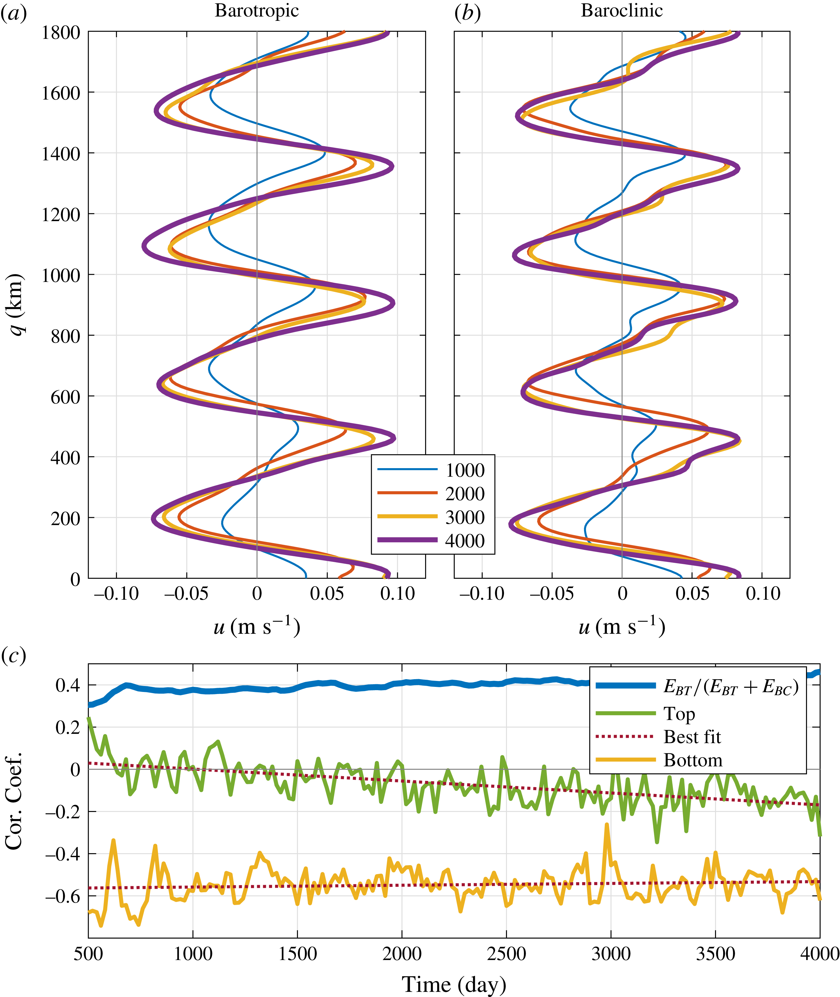
(cross-jet profiles, averaged along the jets, are aligned in the moving frame of reference by assuming a constant drift velocity; note that legend units are in days); and (c) correlation coefficients between the cross-jet profiles of eddy forcing and PV, and the fraction of the total energy in the barotropic component. Here, we used the full flow field to compute the eddy forcing, because it was not possible to compute a mean flow in the transient state.

Moreover, it takes a long time for the system to attain equilibrium. The continuous increase of the total energy (roughly in the interval 1000–4000 days, figure 2
e) is definitely not during the time period when the jets are being formed (§ 2.1), but it has to do with some secondary effects. To investigate this, we first look at the time evolution of the barotropic and baroclinic velocity components in the transient period (figure 8
a,b). Both the barotropic and baroclinic velocity fields increase at similar rates, and, in fact, the ratio of energy in the barotropic component to the total energy (barotropic plus baroclinic,
 $E_{BT}+E_{BC}$
) remains almost constant during this period (blue curve in figure 8
c).
One possible explanation behind this slow energy increase could be the direct forcing by the background flow once the jets are formed. The inertial stress term depends on the mean flow; hence, the linear forcing becomes prominent only after the formation of the jets. Note that the jet formation occurs due to the upscale transfer of energy by mesoscale eddies that receive energy from the background flow. However, at a later stage, the eddies start acting against the linear stress terms and oppose the jets. So, there must be a time interval when the eddies change their behaviour from being jet-supporting to jet-opposing. To confirm this hypothesis, we computed correlation coefficients between the cross-jet eddy forcing and PV profiles during the transient period (figure 8 c). The time evolution of the correlation coefficient shows a decreasing trend in the top layer, where the correlation coefficient changes from a small positive value to negative values with time. On the other hand, the correlation remains negative in the bottom layer. This is probably because the eddy forcing in the bottom layer is largely due to the form stress term, thus producing a negative correlation at all times (also read the discussion of table 3). The results are in accord with our hypothesis, at least in the more active top layer that offers an explanation of the long time scale in the transient period.
4 Conclusions
Interaction of oceanic jets with bottom topography is a problem of interest to many. Here, we studied the effects of zonally sloping bottom topography on the dynamics of multiple alternating jets in oceans in a forced dissipative two-layer nonlinear QG model. In accord with previous studies (Boland et al. Reference Boland, Thompson, Shuckburgh and Haynes2012; Chen et al. Reference Chen, Kamenkovich and Berloff2015), the jets tilt from the zonal direction and drift. We find that the jet drift is strongly controlled by the linear dynamics. The drift velocities are predicted quite accurately with the linear dispersion relation, although the nonlinear eddy effects contribute, and more so for steeper topographic slopes. In the presence of the zonal asymmetry due to the bottom slope, the jets are able to extract energy directly from the imposed background flow, and the forcing term is directly proportional to the developed mean flow. Thus, the linear forcing and mean PV maxima do not align and have a large offset. Because of the off-core linear forcing, the jets are pushed in the meridional direction. If looked at from the point of view of PV conservation, the jets drift meridionally to compensate for the along-jet advection of PV by the mean flow, in agreement with Boland et al. (Reference Boland, Thompson, Shuckburgh and Haynes2012).
On the other hand, the nonlinear eddy forcing does not cause the drift; however, it influences the drift speed by modifying the effective balance between the linear terms. In order to understand the impacts of the eddies, we derived the governing equations in a tilted, non-stationary frame of reference and compared cross-jet profiles of the linear and nonlinear stress terms with the mean PV profile. Here, the eddy forcing is found to be opposing the jets, which is in contrast to the case of stationary zonal jets (Panetta Reference Panetta1993; Berloff et al. Reference Berloff, Kamenkovich and Pedlosky2009a ). The net linear stress term, present in the time-mean equations, directly forces the jets. The eddy forcing was further decomposed into the Reynolds stress term and form stress term. The behaviour of the form stress term is similar to the case of stationary zonal jets over a flat bottom, i.e. the form stress term opposes the jets (Berloff et al. Reference Berloff, Kamenkovich and Pedlosky2009a ). On the other hand, the Reynolds stress term in the upper layer is responsible for forcing the jets (Thompson & Young Reference Thompson and Young2007). Overall, the form stress term dominates and is such that the eddies remove energy from the jets. The gradual transition in the role of eddies from being jet-supporting to being jet-opposing is also confirmed by correlating the cross-jet profiles of the eddy forcing and mean PV anomalies in simulations with different zonal slope magnitudes. The same conclusion was reached when we analysed various eddy fluxes. In the presence of the topography, the eddy buoyancy fluxes oppose the jets in both layers but are much stronger in magnitude than the relative vorticity fluxes, which are jet-supporting. The eddy heat diffusivity, computed from the buoyancy fluxes, is positive everywhere and the maxima occur just south of the eastward jet cores, which may be related to the southward drift of the jets. Overall, the eddy PV fluxes are down-gradient and oppose the jets.
This is in contrast to the conventional point of view that the eddy field maintains the jets – hence the term ‘eddy-driven jets’. We argue, at least in the oceans, that the eddy field can either force or oppose the jets depending on the situation (see e.g. Kamenkovich et al. Reference Kamenkovich, Berloff and Pedlosky2009). Overall, the eddy field allows the jets to reach an equilibrium state. Thus, with regards to oceanic jets, it would be more appropriate to use a term like ‘eddy-sustained jets’. This general eddy effect may not be limited to alternating jets and may be important in other large-scale oceanic flows. For example, eddies play a major role in the dynamics of the Antarctic Circumpolar Current (ACC) (Abernathey & Cessi Reference Abernathey and Cessi2014; Thompson & Naveira Garabato Reference Thompson and Naveira Garabato2014). Recent studies have shown that the behaviour of the Reynolds stress term and form stress term can change abruptly around the topographic features in the Southern Ocean, where, in different parts of the ocean, eddies are seen to be forcing the large-scale flow as well as gaining energy via a barotropic energy source (Barthel et al. Reference Barthel, Hogg, Waterman and Keating2017; Youngs et al. Reference Youngs, Thompson, Lazar and Richards2017).
While examining the total energy of the system, we observed that the flow energy increases with the bottom slope, in agreement with earlier studies (Arbic & Flierl Reference Arbic and Flierl2004; Smith Reference Smith2007; Boland et al. Reference Boland, Thompson, Shuckburgh and Haynes2012). In our study, the eddies gain energy from the baroclinically unstable background flow as well as from the jets, whereas the jets are maintained by the imposed vertical shear. Since both the jets and eddies are forced by the imposed shear, the system tends to be more energetic. It should be noted that the results discussed in this paper are limited to continuously forced dissipative systems and may not apply directly to freely evolving turbulence.
Topography also plays a crucial role in ocean mixing and transport (Tréguier & Panetta Reference Tréguier and Panetta1994; Thompson Reference Thompson2010). Studies on the dynamics of the Southern Ocean have shown enhanced mixing at mid-depths, which is believed to be due to interactions of jets with topography (Abernathey et al. Reference Abernathey, Marshall, Mazloff and Shuckburgh2010; Lu & Speer Reference Lu and Speer2010). Idealised studies have also reported enhanced material transport across tilted, drifting jets (Boland et al. Reference Boland, Thompson, Shuckburgh and Haynes2012; Stern et al. Reference Stern, Nadeau and Holland2015). In fact, a more general question which should be addressed is: What are the effects of the zonal component of PV gradient on the overall dynamics? In reality, the oceans are full of zonal gradients in PV, as the ocean floor is not flat, and, also, the oceans are forced with a wind field having both zonal and meridional components. In this work, we restricted ourselves to a very simple idealised case, but numerical experiments in the presence of a realistic ocean bathymetry forced with an observed wind field are needed to understand the effects in the real oceans. Such studies would shed some light on the role of geostrophic eddies in large-scale ocean mixing and material transport in the presence of topography, and might even be helpful in incorporating topographic impacts in eddy parametrisation schemes. In addition, the effects of continental boundaries could also be analysed. Finally, our dynamical analyses are based on the Reynolds decomposition of the flow into the time-mean (in a non-stationary frame of reference) and fluctuation parts of the flow, and in the future it would be useful to consider other decompositions (e.g. Berloff Reference Berloff2005a ), which are more relevant for parametrising the involved eddy effects in non-eddy-resolving or eddy-permitting models. Further work related to the energetics and stability of the drifting jets is in progress and will be addressed in future.
Acknowledgements
H.K. would like to acknowledge the support from the President’s Scholarship and the Mathematics of Planet Earth CDT, Imperial College. P.B. has been supported by EPSRC Mathematics Platform grant EP/I019111/1 and NERC grant NE/R011567/1. The authors thank I. Kamenkovich and two anonymous reviewers for their comments and suggestions that helped to improve the paper. The authors also thank A. Thompson, I. Shevchenko, N. Constantinou, M. Haigh and M. O’Donnell for their comments on the manuscript. I. Shevchenko also helped with the numerical simulations. The authors would also like to express their gratitude to the HPC team at Imperial College and A. Thomas for their help with computer clusters.
Appendix A. Tilted, drifting jets in a channel simulation
We ran a simulation in a channel configuration and imposed partial-slip boundary conditions on the meridional boundaries, which is given as
 $$\begin{eqnarray}\frac{\unicode[STIX]{x2202}u_{i}}{\unicode[STIX]{x2202}y}+\frac{u_{i}}{\unicode[STIX]{x1D6FC}}=0,\end{eqnarray}$$
where
 $u_{i}$
is the zonal velocity in layer
 $i$
, and
 $\unicode[STIX]{x1D6FC}=120$
km. Here, we used a 7200 km square domain having a grid resolution of
 $2048\times 2049$
, which is just to emphasise that jets tilt and drift irrespective of the domain size and grid resolution. Also,
 $\unicode[STIX]{x1D708}=50~\text{m}^{2}~\text{s}^{-1}$
and
 $\unicode[STIX]{x1D6FE}=10^{-8}~\text{s}^{-1}$
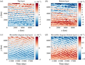
were used to dissipate energy. The rest of the parameters were kept the same as given in § 2.1. The tilted, drifting jets are shown in figure 9. The tilt angle and drift speed are roughly
 $5^{\circ }$
and
 $0.2~\text{cm}~\text{s}^{-1}$
. The dynamics is more complex here, as accumulation of a positive/negative PV anomaly can be seen on the boundaries, which is caused by the drifting jets. A secondary circulation is then created along the boundaries, which transports PV. This way, PV of the system is conserved.
General flow patterns and equilibration of the jets in a channel. (a,b) Snapshots of the PV anomaly (colour bar units are in
 $\text{s}^{-1}$
) field in the top layer (
 $\unicode[STIX]{x1D6FB}^{2}\unicode[STIX]{x1D713}_{1}+S_{1}(\unicode[STIX]{x1D713}_{2}-\unicode[STIX]{x1D713}_{1})$
) and bottom layer (
 $\unicode[STIX]{x1D6FB}^{2}\unicode[STIX]{x1D713}_{2}+S_{2}(\unicode[STIX]{x1D713}_{1}-\unicode[STIX]{x1D713}_{2})$
) for medium-slope configuration. (c,d) Hovmöller diagram of the PV anomaly field in the top and bottom layers (PV along a cross-section at the centre of the domain is plotted against time).

Appendix B. Dispersion relation in the two-layer QG model
The dispersion relation is derived by substituting
 $\unicode[STIX]{x1D713}_{i}=\widetilde{\unicode[STIX]{x1D713}}_{i}\text{e}^{\text{i}(kx+ly-\unicode[STIX]{x1D714}t)}$
in (2.1) and (2.2). The resulting linearised equations can be represented in the following matrix form:
 $$\begin{eqnarray}\!\left[\begin{array}{@{}cc@{}}\unicode[STIX]{x1D714}(k^{2}+l^{2}+S_{1})+k(\unicode[STIX]{x1D6FD}-U_{b}(k^{2}+l^{2})) & -S_{1}\unicode[STIX]{x1D714}+S_{1}U_{b}k\\ +\,\text{i}\unicode[STIX]{x1D708}(k^{4}+l^{4})\hspace{60.0pt} & \\ -S_{2}\unicode[STIX]{x1D714} & \unicode[STIX]{x1D714}(k^{2}+l^{2}+S_{2})-lT_{x}+k(\unicode[STIX]{x1D6FD}-U_{b}S_{2})\\ & +\,\text{i}\unicode[STIX]{x1D708}(k^{4}+l^{4})+\text{i}\unicode[STIX]{x1D6FE}(l^{2}+l^{2})\\ \end{array}\right]\!\left[\begin{array}{@{}c@{}}\widetilde{\unicode[STIX]{x1D713}}_{1}\\ \widetilde{\unicode[STIX]{x1D713}}_{2}\end{array}\right]=0.\end{eqnarray}$$
For the existence of non-trivial solutions, the determinant of the matrix must vanish, which results in two frequency solutions for each wavenumber pair (
 $k,l$
). The real parts of the frequencies predict two different drift velocities, which are in opposite directions and possess different magnitudes, corresponding to the wavenumber. For the purpose of comparing drift velocities, the frequency solution giving the same direction of drift as the jets in the simulations is considered. It turns out that the chosen frequency also predicts faster drift out of the two frequencies.
Appendix C. Derivation of the QG equations in a tilted, non-stationary frame of reference
From (3.1) and (3.2), the variables can be represented as a sum of the time-mean (
 $\overline{Q}_{i}$
,
 $\overline{\unicode[STIX]{x1D713}}_{i}$
) and eddy components (
 $Q_{i}^{\prime }$
,
 $\unicode[STIX]{x1D713}_{i}^{\prime }$
):
 $$\begin{eqnarray}\displaystyle & & \displaystyle \left[\frac{\unicode[STIX]{x2202}}{\unicode[STIX]{x2202}t}-c\frac{\unicode[STIX]{x2202}}{\unicode[STIX]{x2202}q}\right](\overline{Q}_{1}+Q_{1}^{\prime })\nonumber\\ \displaystyle & & \displaystyle \quad =-\left(\frac{\unicode[STIX]{x2202}(\overline{\unicode[STIX]{x1D713}}_{1}+\unicode[STIX]{x1D713}_{1}^{\prime })}{\unicode[STIX]{x2202}p}-U_{b}\sin \unicode[STIX]{x1D703}\right)\left(\frac{\unicode[STIX]{x2202}(\overline{Q}_{1}+Q_{1}^{\prime })}{\unicode[STIX]{x2202}q}+(\unicode[STIX]{x1D6FD}+S_{1}U_{b})\cos \unicode[STIX]{x1D703}\right)\nonumber\\ \displaystyle & & \displaystyle \qquad +\left(\frac{\unicode[STIX]{x2202}(\overline{\unicode[STIX]{x1D713}}_{1}+\unicode[STIX]{x1D713}_{1}^{\prime })}{\unicode[STIX]{x2202}q}-U_{b}\cos \unicode[STIX]{x1D703}\right)\left(\frac{\unicode[STIX]{x2202}(\overline{Q}_{1}+Q_{1}^{\prime })}{\unicode[STIX]{x2202}p}+(\unicode[STIX]{x1D6FD}+S_{1}U_{b})\sin \unicode[STIX]{x1D703}\right)\nonumber\\ \displaystyle & & \displaystyle \qquad +\,\unicode[STIX]{x1D708}\unicode[STIX]{x1D6FB}^{4}(\overline{\unicode[STIX]{x1D713}}_{1}+\unicode[STIX]{x1D713}_{1}^{\prime }),\end{eqnarray}$$
 $$\begin{eqnarray}\displaystyle \displaystyle \left[\frac{\unicode[STIX]{x2202}}{\unicode[STIX]{x2202}t}-c\frac{\unicode[STIX]{x2202}}{\unicode[STIX]{x2202}q}\right](\overline{Q}_{2}+Q_{2}^{\prime }) & = & \displaystyle -\frac{\unicode[STIX]{x2202}(\overline{\unicode[STIX]{x1D713}}_{2}+\unicode[STIX]{x1D713}_{2}^{\prime })}{\unicode[STIX]{x2202}p}\left(\frac{\unicode[STIX]{x2202}(\overline{Q}_{2}+Q_{2}^{\prime })}{\unicode[STIX]{x2202}q}+(\unicode[STIX]{x1D6FD}-S_{2}U_{b})\cos \unicode[STIX]{x1D703}-T_{x}\sin \unicode[STIX]{x1D703}\right)\nonumber\\ \displaystyle & & \displaystyle +\,\frac{\unicode[STIX]{x2202}(\overline{\unicode[STIX]{x1D713}}_{2}+\unicode[STIX]{x1D713}_{2}^{\prime })}{\unicode[STIX]{x2202}q}\left(\frac{\unicode[STIX]{x2202}(\overline{Q}_{2}+Q_{2}^{\prime })}{\unicode[STIX]{x2202}p}+(\unicode[STIX]{x1D6FD}-S_{2}U_{b})\sin \unicode[STIX]{x1D703}+T_{x}\cos \unicode[STIX]{x1D703}\right)\hspace{-6.0pt}\nonumber\\ \displaystyle & & \displaystyle +\,\unicode[STIX]{x1D708}\unicode[STIX]{x1D6FB}^{4}(\overline{\unicode[STIX]{x1D713}}_{2}+\unicode[STIX]{x1D713}_{2}^{\prime })-\unicode[STIX]{x1D6FE}\unicode[STIX]{x1D6FB}^{2}(\overline{\unicode[STIX]{x1D713}}_{2}+\unicode[STIX]{x1D713}_{2}^{\prime }).\end{eqnarray}$$
The equations are then averaged over time to derive the time-mean equations. Note that
 $\overline{Q_{i}^{\prime }}=\overline{\unicode[STIX]{x1D713}_{i}^{\prime }}=0$
and
 $\unicode[STIX]{x2202}\overline{Q_{i}}/\unicode[STIX]{x2202}p=\unicode[STIX]{x2202}\overline{\unicode[STIX]{x1D713}_{i}}/\unicode[STIX]{x2202}p=0$
(the jets are purely zonal in the new configuration). Thus
 $$\begin{eqnarray}\displaystyle \displaystyle \frac{\unicode[STIX]{x2202}\overline{Q}_{1}}{\unicode[STIX]{x2202}t}-c\frac{\unicode[STIX]{x2202}\overline{Q}_{1}}{\unicode[STIX]{x2202}q} & = & \displaystyle -\overline{\frac{\unicode[STIX]{x2202}\unicode[STIX]{x1D713}_{1}^{\prime }}{\unicode[STIX]{x2202}p}\frac{\unicode[STIX]{x2202}Q_{1}^{\prime }}{\unicode[STIX]{x2202}q}}+U_{b}\sin \unicode[STIX]{x1D703}\frac{\unicode[STIX]{x2202}\overline{Q}_{1}}{\unicode[STIX]{x2202}q}+\overline{\frac{\unicode[STIX]{x2202}\unicode[STIX]{x1D713}_{1}^{\prime }}{\unicode[STIX]{x2202}q}\frac{\unicode[STIX]{x2202}Q_{1}^{\prime }}{\unicode[STIX]{x2202}p}}\nonumber\\ \displaystyle & & \displaystyle +\,(\unicode[STIX]{x1D6FD}+S_{1}U_{b})\sin \unicode[STIX]{x1D703}\frac{\unicode[STIX]{x2202}\overline{\unicode[STIX]{x1D713}_{1}}}{\unicode[STIX]{x2202}q}+\unicode[STIX]{x1D708}\unicode[STIX]{x1D6FB}^{4}\overline{\unicode[STIX]{x1D713}}_{1},\end{eqnarray}$$
 $$\begin{eqnarray}\displaystyle \displaystyle \frac{\unicode[STIX]{x2202}\overline{Q}_{2}}{\unicode[STIX]{x2202}t}-c\frac{\unicode[STIX]{x2202}\overline{Q}_{2}}{\unicode[STIX]{x2202}q} & = & \displaystyle -\overline{\frac{\unicode[STIX]{x2202}\unicode[STIX]{x1D713}_{2}^{\prime }}{\unicode[STIX]{x2202}p}\frac{\unicode[STIX]{x2202}Q_{2}^{\prime }}{\unicode[STIX]{x2202}q}}+\overline{\frac{\unicode[STIX]{x2202}\unicode[STIX]{x1D713}_{2}^{\prime }}{\unicode[STIX]{x2202}q}\frac{\unicode[STIX]{x2202}Q_{2}^{\prime }}{\unicode[STIX]{x2202}p}}+\left[(\unicode[STIX]{x1D6FD}-S_{2}U_{b})\sin \unicode[STIX]{x1D703}\right.\nonumber\\ \displaystyle & & \displaystyle \left.+\,T_{x}\cos \unicode[STIX]{x1D703}\right]\frac{\unicode[STIX]{x2202}\overline{\unicode[STIX]{x1D713}_{2}}}{\unicode[STIX]{x2202}q}+\unicode[STIX]{x1D708}\unicode[STIX]{x1D6FB}^{4}\overline{\unicode[STIX]{x1D713}}_{2}-\unicode[STIX]{x1D6FE}\unicode[STIX]{x1D6FB}^{2}\overline{\unicode[STIX]{x1D713}}_{2}.\end{eqnarray}$$
For clarity, we retain the time derivatives in the mean PV. In equilibrium, the time derivative terms vanish. We then replace the streamfunction by velocity (
 $\boldsymbol{u}_{i}=(u_{i},v_{i})=(-\unicode[STIX]{x2202}\unicode[STIX]{x1D713}_{i}/\unicode[STIX]{x2202}q,\unicode[STIX]{x2202}\unicode[STIX]{x1D713}_{i}/\unicode[STIX]{x2202}p)$
), introduce relative vorticity (
 $\unicode[STIX]{x1D701}_{i}=\unicode[STIX]{x1D6FB}^{2}\unicode[STIX]{x1D713}_{i}$
), and represent the nonlinear terms in the flux form (note that
 $\unicode[STIX]{x1D735}\boldsymbol{\cdot }\boldsymbol{u}_{i}^{\prime }=0$
from the continuity equation). The final time-mean equations are given as
 $$\begin{eqnarray}\displaystyle & \displaystyle \frac{\unicode[STIX]{x2202}\overline{Q}_{1}}{\unicode[STIX]{x2202}t}=-\unicode[STIX]{x1D735}\boldsymbol{\cdot }\overline{(\boldsymbol{u}_{1}^{\prime }Q_{1}^{\prime })}+(c+U_{b}\sin \unicode[STIX]{x1D703})\frac{\unicode[STIX]{x2202}\overline{Q}_{1}}{\unicode[STIX]{x2202}q}-(\unicode[STIX]{x1D6FD}+S_{1}U_{b})\sin \unicode[STIX]{x1D703}\,\,\overline{u}_{1}+\unicode[STIX]{x1D708}\unicode[STIX]{x1D6FB}^{2}\overline{\unicode[STIX]{x1D701}}_{1},\qquad & \displaystyle\end{eqnarray}$$
 $$\begin{eqnarray}\displaystyle & \displaystyle \frac{\unicode[STIX]{x2202}\overline{Q}_{2}}{\unicode[STIX]{x2202}t}=-\unicode[STIX]{x1D735}\boldsymbol{\cdot }\overline{(\boldsymbol{u}_{2}^{\prime }Q_{2}^{\prime })}+c\frac{\unicode[STIX]{x2202}\overline{Q}_{2}}{\unicode[STIX]{x2202}q}-[(\unicode[STIX]{x1D6FD}-S_{2}U_{b})\sin \unicode[STIX]{x1D703}+T_{x}\cos \unicode[STIX]{x1D703}]\,\overline{u}_{2}+\unicode[STIX]{x1D708}\unicode[STIX]{x1D6FB}^{2}\overline{\unicode[STIX]{x1D701}}_{2}-\unicode[STIX]{x1D6FE}\overline{\unicode[STIX]{x1D701}}_{2}.\qquad & \displaystyle\end{eqnarray}$$