1 Introduction
Turbulent flows laden with particles or droplets are common phenomena in various natural and engineering applications, such as atmospheric dispersal of pollutants, pulverized coal in furnaces and liquid sprays in engines. These areas involve turbulence modulation in the carrier phase, as well as dispersion and polydispersity of the dispersed phase, which are very important and complicated issues in multiphase flows. When the turbulence is highly compressible, the rotational motion and the compressibility of fluid are both significant. Besides, eddy shocklets can also exist in the carrier phase, which makes the problems of two-way coupled turbulent flows more complex. Researches on the mechanisms of the complex interactions between particles and compressible turbulence are very meaningful, which can promote the understandings of multiphase flows and ultimately improve the industrial devices involving these flows.
Isotropic turbulence is the simplest and representative turbulence, which are extensively used to study turbulence modulation by particles. In the past decades, turbulence modulation by dispersed particles are mostly conducted in incompressible isotropic turbulence based on direct numerical simulations (DNSs) with the Eulerian–Lagrangian point-source approach, where the diameter of particles is smaller than the Kolmogorov length scale. Ferrante & Elghobashi (Reference Ferrante and Elghobashi2003) studied the physical mechanisms of the modulation to decaying isotropic turbulence by dispersed particles, and found that microparticles (the initial Stokes number of particles
 $St_{0}\ll 1$
) would augment turbulence and the rotational motion of fluid, while large particles (
 $St_{0}>1$
) would attenuate turbulence and the rotational motion of fluid. In addition, they also found that the kinetic energy spectrum was attenuated at low wavenumbers and augmented at high wavenumbers. Boivin, Simonin & Squires (Reference Boivin, Simonin and Squires1998) investigated turbulence modulation in stationary isotropic turbulence, where the attenuation of the turbulent kinetic energy and dissipation rate was observed, and the kinetic energy spectrum was attenuated at low wavenumbers and augmented at high wavenumbers. Abdelsamie & Lee (Reference Abdelsamie and Lee2012, Reference Abdelsamie and Lee2013) clarified the distinction of turbulence modulation between decaying turbulence and stationary turbulence through investigating the turbulence modulation mechanisms and heavy particles statistics. They found turbulence modulation in decaying turbulence is qualitatively and quantitatively discrepant from that in stationary turbulence for microparticles, while they were qualitatively similar for large particles. Furthermore, they concluded that stationary turbulence was not appropriate for the research of turbulence modulation by microparticles owing to the artificial forcing therein.
Different from incompressible turbulence, temperature, pressure and other thermodynamic quantities fluctuate sharply in some cases such as hypersonic aircrafts’ engines and interstellar clouds, where the compressibility of the flow field cannot be neglected. Compressible turbulence, especially for those with high turbulent Mach number (
 $M_{t}$
), is more complicated compared with the incompressible turbulence, because of the nonlinear interactions between the velocity field and the pressure field, as well as the existence of shocklets. Passot & Pouquet (Reference Passot and Pouquet1987) simulated a two-dimensional compressible homogeneous turbulence with high Mach number, and found shocklets existed in the field when
 $M_{t}>0.3$
. Samtaney, Pullin & Kosović (Reference Samtaney, Pullin and Kosović2001) used a tenth-order compact finite difference scheme to study decaying compressible isotropic turbulence with direct numerical simulations, and analysed the influence of turbulent Mach number and Taylor Reynolds number on random shocklets in the flow field. Wang et al. (Reference Wang, Shi, Wang, Xiao, He and Chen2011, Reference Wang, Shi, Wang, Xiao, He and Chen2012a
,Reference Wang, Shi, Wang, Xiao and He
b
, Reference Wang, Yang, Shi, Xiao, He and Chen2013) simulated a highly compressible forced isotropic turbulence with turbulent Mach number around 1.0, and investigated the scaling and statistical properties, the effect of shocklets on the velocity gradients and the effect of compressibility on the small-scale structures.
Although research on incompressible two-phase turbulence and compressible one-phase turbulence have made great progress over the past decades, there are few studies on compressible two-phase turbulence, especially those with high turbulent Mach number. Xia et al. (Reference Xia, Shi, Zhang and Chen2016) studied modifications of forced compressible homogenous turbulence by heavy point particles with different particle densities, where the turbulent Mach number is around 1.0, and analysed the influence of particle densities on the statistics of the turbulence. They found that turbulence was suppressed by particles and the suppression was more obvious when the density of particles increased, which is similar to that in forced incompressible turbulence. However, the underlying turbulence modulation mechanism was not clarified. Zhang et al. (Reference Zhang, Liu, Ma and Xiao2016) investigated the preferential concentration of heavy particles in stationary compressible isotropic turbulence with one-way coupling, and found particles tended to collect in high-density and low-vorticity regions. Critical particles with
 $St=1.0$
were also found to accumulate in high-vorticity regions behind the shocklets. As the turbulent Mach number decreased, the degree of particle clustering in high-vorticity regions was weakened.
So far, turbulence modulation by small inertia particles in compressible turbulence has not been completely understood, especially when the turbulent Mach number is high. In particular, the interaction between particles and decaying compressible isotropic turbulence has not been investigated, and the modifications of the compressibility in the turbulence filed remain unknown. Therefore, it is of great importance to perform the investigation of turbulence modulation by particles in decaying compressible isotropic turbulence.
In the present work, we apply direct numerical simulations with the Eulerian–Lagrangian point-source method to investigate turbulence modulation by inertia particles in compressible isotropic turbulence. The diameter of particles is smaller than the Kolmogorov length scale and particles interact with turbulence through two-way coupling. As stationary turbulence is not appropriate for the study of turbulence modulation, especially for particles with
 $St\leqslant 1$
(Lucci, Ferrante & Elghobashi Reference Lucci, Ferrante and Elghobashi2010; Abdelsamie & Lee Reference Abdelsamie and Lee2012), we employ decaying turbulence to avoid the influence of the artificial forcing. The initial turbulent Mach number is up to 1.2 and the Taylor Reynolds number is 51.7. Five different simulations with different particle diameters (or initial Stokes numbers) are conducted. The main objectives of the present work is to investigate the modifications of turbulent features, compressibility and energy spectra of the flow field by particles, as well as analyse the compressible turbulence modulation mechanism.
2 Numerical approaches
2.1 Governing equations of the fluid flow
The carrier phase is supposed to be compressible Newtonian fluid, so the governing equations of the carrier phase employ the Eulerian forms of three-dimensional compressible Navier–Stokes equations, which include the conservation equations of continuity, momentum and energy, as well as the state equation.
The governing equations are non-dimensionalized based on the following characteristic parameters:
 $L_{0}$
for length,
 $u_{0}$
for velocity,
 $L_{0}/u_{0}$
for time,
 $T_{0}$
for temperature,
 $\unicode[STIX]{x1D70C}_{0}$
for density,
 $c_{0}$
for the speed of sound (
 $c_{0}=\sqrt{\unicode[STIX]{x1D6FE}RT_{0}}$
for an ideal gas, where
 $\unicode[STIX]{x1D6FE}=C_{p}/C_{v}$
is the ratio of specific heat at constant pressure
 $C_{p}$
to that at constant volume
 $C_{v}$
and
 $R=C_{p}-C_{v}$
is the specific gas constant),
 $p_{0}=\unicode[STIX]{x1D70C}_{0}c_{0}^{2}/\unicode[STIX]{x1D6FE}$
for pressure,
 $\unicode[STIX]{x1D70C}_{0}u_{0}^{2}$
for energy per unit volume,
 $\unicode[STIX]{x1D707}_{0}$
for dynamic viscosity and
 $\unicode[STIX]{x1D705}_{0}$
for conductivity. Therefore, the dimensionless governing equations can be formulated as
 $$\begin{eqnarray}\displaystyle & \displaystyle \frac{\unicode[STIX]{x2202}\unicode[STIX]{x1D70C}}{\unicode[STIX]{x2202}t}+\frac{\unicode[STIX]{x2202}(\unicode[STIX]{x1D70C}u_{j})}{\unicode[STIX]{x2202}x_{j}}=0, & \displaystyle\end{eqnarray}$$
 $$\begin{eqnarray}\displaystyle & \displaystyle \frac{\unicode[STIX]{x2202}(\unicode[STIX]{x1D70C}u_{i})}{\unicode[STIX]{x2202}t}+\frac{\unicode[STIX]{x2202}[\unicode[STIX]{x1D70C}u_{i}u_{j}+p_{m}\unicode[STIX]{x1D6FF}_{ij}]}{\unicode[STIX]{x2202}x_{j}}=\frac{1}{Re}\frac{\unicode[STIX]{x2202}\unicode[STIX]{x1D70E}_{ij}}{\unicode[STIX]{x2202}x_{j}}+\unicode[STIX]{x1D711}_{ui}, & \displaystyle\end{eqnarray}$$
 $$\begin{eqnarray}\displaystyle & \displaystyle \frac{\unicode[STIX]{x2202}E}{\unicode[STIX]{x2202}t}+\frac{\unicode[STIX]{x2202}[(E+p_{m})u_{j}]}{\unicode[STIX]{x2202}x_{j}}=\frac{1}{\unicode[STIX]{x1D6FC}}\frac{\unicode[STIX]{x2202}}{\unicode[STIX]{x2202}x_{j}}\left(k\frac{\unicode[STIX]{x2202}T}{\unicode[STIX]{x2202}x_{j}}\right)+\frac{1}{Re}\frac{\unicode[STIX]{x2202}(\unicode[STIX]{x1D70E}_{ij}u_{i})}{\unicode[STIX]{x2202}x_{j}}+\unicode[STIX]{x1D711}_{e}, & \displaystyle\end{eqnarray}$$
 $$\begin{eqnarray}\displaystyle & \displaystyle p=\unicode[STIX]{x1D70C}T. & \displaystyle\end{eqnarray}$$
Here,
 $u_{i}$
,
 $\unicode[STIX]{x1D70C}$
,
 $p$
and
 $T$
are dimensionless velocity, density, pressure and temperature respectively. The ideal gas model is used for the thermodynamic equation of state. The modified pressure
 $p_{m}$
, viscous stress
 $\unicode[STIX]{x1D70E}_{ij}$
and total energy per unit volume
 $E$
are defined as
 $$\begin{eqnarray}p_{m}=\frac{p}{\unicode[STIX]{x1D6FE}M^{2}},\quad \unicode[STIX]{x1D70E}_{ij}=\unicode[STIX]{x1D707}\left(\frac{\unicode[STIX]{x2202}u_{i}}{\unicode[STIX]{x2202}x_{j}}+\frac{\unicode[STIX]{x2202}u_{j}}{\unicode[STIX]{x2202}x_{i}}\right)-\frac{2}{3}\unicode[STIX]{x1D707}\unicode[STIX]{x1D703}\unicode[STIX]{x1D6FF}_{ij},\end{eqnarray}$$
 $$\begin{eqnarray}E=\frac{p}{(\unicode[STIX]{x1D6FE}-1)\unicode[STIX]{x1D6FE}M^{2}}+\frac{1}{2}\unicode[STIX]{x1D70C}u_{j}u_{j},\end{eqnarray}$$
where
 $\unicode[STIX]{x1D703}=\unicode[STIX]{x2202}u_{k}/\unicode[STIX]{x2202}x_{k}$
is the dimensionless velocity divergence or dilatation. The other dimensionless characteristic parameters in the governing equations are as followings: Prandtl number
 $Pr=\unicode[STIX]{x1D707}_{0}C_{p}/\unicode[STIX]{x1D705}_{0}$
, Reynolds number
 $Re=\unicode[STIX]{x1D70C}_{0}u_{0}L_{0}/\unicode[STIX]{x1D707}_{0}$
, Mach number
 $M=u_{0}/c_{0}$
and
 $\unicode[STIX]{x1D6FC}=Pr\,Re(\unicode[STIX]{x1D6FE}-1)M^{2}$
. The dimensionless dynamic viscosity
 $\unicode[STIX]{x1D707}$
and dimensionless thermal conductivity
 $\unicode[STIX]{x1D705}$
are associated with temperature, and computed by the Sutherland law (Sutherland Reference Sutherland1893) as
 $$\begin{eqnarray}\unicode[STIX]{x1D707}=\unicode[STIX]{x1D705}=\frac{1.40417T^{1.5}}{T+0.40417}.\end{eqnarray}$$
The effects of particles on the fluid are considered through the source terms
 $\unicode[STIX]{x1D711}_{ui}$
and
 $\unicode[STIX]{x1D711}_{e}$
which describe the momentum and energy contributions from particles.
2.2 Governing equations of particle motion
It is assumed that particles are solid spheres with identical diameter
 $d_{p}$
, temperature
 $t_{p}$
and density
 $\unicode[STIX]{x1D70C}_{p}$
in a specific case. Gravitational settling, inter-particle collisions and heat transfer between turbulence and particles are negligible. The trajectories of particles are tracked in the Lagrangian manner and follow the Basset–Boussinesq–Oseeen equations in compressible flow (Parmar, Haselbacher & Balachandar Reference Parmar, Haselbacher and Balachandar2012). Since the density of particles is much larger than that of the fluid at the particle positions
 $(\unicode[STIX]{x1D70C}_{p}/\unicode[STIX]{x1D70C}_{f}\approx 1000)$
, only the Stokes drag force is significant. The buoyancy force, the pressure-gradient force, the Basset force, the virtual-mass force and other unsteady drag forces can be neglected since they are all much smaller than the Stokes drag force (Crowe, Sommerfeld & Tsuji Reference Crowe, Sommerfeld and Tsuji1998). Therefore, the governing equations for each particle motion can be given by
 $$\begin{eqnarray}\displaystyle & \displaystyle \frac{\text{d}x_{p,i}}{\text{d}t}=v_{p,i}, & \displaystyle\end{eqnarray}$$
 $$\begin{eqnarray}\displaystyle & \displaystyle \frac{\text{d}v_{p,i}}{\text{d}t}=\frac{F_{p,i}}{m_{p}}=\frac{f_{1}}{\unicode[STIX]{x1D70F}_{p}}(u_{p,i}-v_{p,i}). & \displaystyle\end{eqnarray}$$
Here,
 $x_{p,i}$
is the particle displacement,
 $v_{p,i}$
is the particle velocity,
 $u_{p,i}$
is the fluid velocity at the particle position,
 $F_{p,i}$
is the Stokes drag force acting on the particle,
 $\unicode[STIX]{x1D70F}_{p}$
is the particle relaxation time which is defined as
 $\unicode[STIX]{x1D70F}_{p}=Re\unicode[STIX]{x1D70C}_{p}d_{p}^{2}/(18\unicode[STIX]{x1D707})$
and
 $m_{p}$
is the mass of an individual particle which is computed by
 $m_{p}=\unicode[STIX]{x03C0}d_{p}^{3}\unicode[STIX]{x1D70C}_{p}/6$
.
 $f_{1}$
is the empirical correction to the Stokes drag force which is expressed as
 $$\begin{eqnarray}f_{1}=1+0.15Re_{p,slip}^{0.687},\end{eqnarray}$$
where
 $Re_{p,slip}=Re\unicode[STIX]{x1D70C}|u_{p,i}-v_{p,i}|d_{p}/\unicode[STIX]{x1D707}$
is the relative particle Reynolds number based on the slip velocity between the particle and the fluid. Since the relative particle Mach number
 $M_{p}=|u_{p,i}-v_{p,i}|/c_{p}$
is small, where
 $c_{p}$
is the speed of gas sound at the particle position, the compressibility correction is neglected in our numerical simulations (Zhang et al.
Reference Zhang, Liu, Ma and Xiao2016).
2.3 Coupling terms between the fluid and the particles
The momentum and energy couplings between the particles and the carrier fluid are shown as the momentum source term
 $\unicode[STIX]{x1D711}_{ui}$
and the energy source term
 $\unicode[STIX]{x1D711}_{e}$
in the governing equations of the fluid flow. Based on the point source in cell (PSIC) assumption, the source terms are calculated from the Lagrangian particle variables by volume averaging the contributions from all the particles existing in the computational cell centred on each grid point, which are given by
 $$\begin{eqnarray}\displaystyle & \displaystyle \unicode[STIX]{x1D711}_{ui}=-\frac{1}{\unicode[STIX]{x0394}V}\mathop{\sum }_{n_{p}}F_{p,i}, & \displaystyle\end{eqnarray}$$
 $$\begin{eqnarray}\displaystyle & \displaystyle \unicode[STIX]{x1D711}_{e}=-\frac{1}{\unicode[STIX]{x0394}V}\mathop{\sum }_{n_{p}}F_{p,i}v_{p,i}, & \displaystyle\end{eqnarray}$$
where
 $n_{p}$
is the number of particles residing within each computational cell and
 $\unicode[STIX]{x0394}V$
is the volume of the computational cell.
2.4 Fundamental parameters definition
In this section, some fundamental parameters of the compressible isotropic turbulence are defined as follows (Wang et al.
Reference Wang, Shi, Wang, Xiao, He and Chen2012a
; Xia et al.
Reference Xia, Shi, Zhang and Chen2016). The root mean square (r.m.s.) of the fluctuation velocity magnitude is defined as
 $u=\sqrt{\langle u_{1}^{2}+u_{2}^{2}+u_{3}^{2}\rangle }$
, where
 $\langle \rangle$
indicates the Eulerian ensemble average over the number of grid points. The turbulent kinetic energy is
 $E_{k}=\langle \unicode[STIX]{x1D70C}u_{i}u_{i}\rangle /2$
, the internal energy is
 $E_{i}=\langle p\rangle /[(\unicode[STIX]{x1D6FE}-1)\unicode[STIX]{x1D6FE}M^{2}]$
, and the total energy is
 $E=E_{k}+E_{i}$
. The vorticity magnitude is computed by
 $$\begin{eqnarray}\unicode[STIX]{x1D714}=\sqrt{(\unicode[STIX]{x1D714}_{1}^{2}+\unicode[STIX]{x1D714}_{2}^{2}+\unicode[STIX]{x1D714}_{3}^{2})},\end{eqnarray}$$
where
 $\unicode[STIX]{x1D714}_{1}=\unicode[STIX]{x2202}u_{3}/\unicode[STIX]{x2202}x_{2}-\unicode[STIX]{x2202}u_{2}/\unicode[STIX]{x2202}x_{3}$
is vorticity in the
 $x_{1}$
direction,
 $\unicode[STIX]{x1D714}_{2}=\unicode[STIX]{x2202}u_{1}/\unicode[STIX]{x2202}x_{3}-\unicode[STIX]{x2202}u_{3}/\unicode[STIX]{x2202}x_{1}$
is vorticity in the
 $x_{2}$
direction and
 $\unicode[STIX]{x1D714}_{3}=\unicode[STIX]{x2202}u_{2}/\unicode[STIX]{x2202}x_{1}-\unicode[STIX]{x2202}u_{1}/\unicode[STIX]{x2202}x_{2}$
is vorticity in the
 $x_{3}$
direction.
Two fundamental parameters are adopted to characterize the flow filed, which are the Taylor Reynolds number and the turbulent Mach number, expressed as
 $$\begin{eqnarray}\displaystyle & \displaystyle Re_{\unicode[STIX]{x1D706}}=Re\frac{u\unicode[STIX]{x1D706}\langle \unicode[STIX]{x1D70C}\rangle }{\sqrt{3}\langle \unicode[STIX]{x1D707}\rangle }, & \displaystyle\end{eqnarray}$$
 $$\begin{eqnarray}\displaystyle & \displaystyle M_{t}=M\frac{u}{\sqrt{T}}, & \displaystyle\end{eqnarray}$$
where the Taylor microscale is
 $$\begin{eqnarray}\unicode[STIX]{x1D706}=\sqrt{\frac{u^{2}}{\langle (\unicode[STIX]{x2202}u_{1}/\unicode[STIX]{x2202}x_{1})^{2}+(\unicode[STIX]{x2202}u_{2}/\unicode[STIX]{x2202}x_{2})^{2}+(\unicode[STIX]{x2202}u_{3}/\unicode[STIX]{x2202}x_{3})^{2}\rangle }}.\end{eqnarray}$$
The energy spectrum of the velocity field is given by
 $$\begin{eqnarray}E(k)=\mathop{\sum }_{k\leqslant |\boldsymbol{k}|<k+1}|\hat{\boldsymbol{u}}(\boldsymbol{k})|^{2}/2,\end{eqnarray}$$
where
 $\boldsymbol{k}$
is the coordinate in the wavenumber space,
 $k=|\boldsymbol{k}|$
is the wavenumber and
 $\hat{\boldsymbol{u}}$
is the field in the wavenumber space obtained through the Fourier transform of the velocity field
 $\boldsymbol{u}$
. Based on the energy spectrum
 $E(k)$
, the integral length scale of the velocity field can be calculated by
 $$\begin{eqnarray}L_{f}=\frac{3\unicode[STIX]{x03C0}}{4}\frac{\displaystyle \int _{0}^{\infty }[E(k)/k]\,\text{d}k}{\displaystyle \int _{0}^{\infty }E(k)\,\text{d}k},\end{eqnarray}$$
which reflects the characteristic length scale of the large vortical structure in the turbulence field. As a result, the large eddy turnover time is
 $\unicode[STIX]{x1D70F}=\sqrt{3}L_{f}/u$
.
The Kolmogorov length scale (dissipation scale) of the flow field is expressed as
 $\unicode[STIX]{x1D702}=[\langle \unicode[STIX]{x1D707}/(Re\unicode[STIX]{x1D70C})\rangle ^{3}/(\unicode[STIX]{x1D700}/\unicode[STIX]{x1D70C})]^{1/4}$
, where
 $\unicode[STIX]{x1D700}=\langle \unicode[STIX]{x1D70E}_{ij}(\unicode[STIX]{x2202}u_{i}/\unicode[STIX]{x2202}x_{j})/Re\rangle$
is the viscous dissipation rate. So the Kolmogorov time scale is given by
 $\unicode[STIX]{x1D70F}_{\unicode[STIX]{x1D702}}=\sqrt{\langle \unicode[STIX]{x1D707}/(Re\unicode[STIX]{x1D70C})\rangle /(\unicode[STIX]{x1D700}/\unicode[STIX]{x1D70C})}$
.
For particles, the Stokes number is defined as the ratio of the particle relaxation time to the Kolmogorov time scale, which is expressed as
 $$\begin{eqnarray}St=\frac{\unicode[STIX]{x1D70F}_{p}}{\unicode[STIX]{x1D70F}_{\unicode[STIX]{x1D702}}}.\end{eqnarray}$$
The volume fraction and mass fraction of particles are given by
 $$\begin{eqnarray}\displaystyle & \displaystyle \unicode[STIX]{x1D719}_{v}=N_{p}V_{p}/V_{f}, & \displaystyle\end{eqnarray}$$
 $$\begin{eqnarray}\displaystyle & \displaystyle \unicode[STIX]{x1D719}_{m}=\unicode[STIX]{x1D70C}_{p}N_{p}V_{p}/\unicode[STIX]{x1D70C}V_{f}, & \displaystyle\end{eqnarray}$$
where
 $N_{p}$
is the total number of particles,
 $V_{p}=\unicode[STIX]{x03C0}d_{p}^{3}/6$
is the volume of an individual particle and
 $V_{f}=(2\unicode[STIX]{x03C0})^{3}$
is the volume of the whole flow field.
3 Computational methodology and initializations
In this work, the Eulerian–Lagrangian point-source method is applied to investigate the two-way coupling interactions between inertia particles and compressible isotropic turbulence. As shocklets would be generated in the flow field, the eighth-order accurate bandwidth-optimized weighted essentially non-oscillatory (WENO-BO4) scheme (Martín et al. Reference Martín, Taylor, Wu and Weirs2006) is employed to discrete the convective terms of the Navier–Stokes equations. The eighth-order standard central difference scheme (Kennedy & Carpenter Reference Kennedy and Carpenter1994) is adopted to calculate the viscous terms. Besides, the third-order total variation diminishing (TVD) Runge–Kutta multistage method (Shu & Osher Reference Shu and Osher1988) is used for the time integrations. To avoid non-physical oscillations near the shocklets in the carrier phase, we adopt the trilinear interpolation scheme to compute the fluid velocity at the particle locations (Xia et al. Reference Xia, Shi, Zhang and Chen2016). And the same third-order TVD Runge–Kutta multistage method is used for the time integrations of the particle motion equations (Davis et al. Reference Davis, Dittmann, Jacobs and Don2011).
The computational domain is a periodic box
 $(2\unicode[STIX]{x03C0})^{3}$
full of compressible viscous fluid. A resolution of
 $128^{3}$
uniform grid is applied with the size
 $\text{d}x=\text{d}y=\text{d}z=0.049$
. The time step is
 $\unicode[STIX]{x0394}t=0.002$
and each simulation runs 10 000 time steps until the non-dimensional time
 $t=20$
. The dimensionless characteristic parameters are given by
 $Re=547.673$
,
 $M=3.673$
,
 $Pr=0.7$
and
 $\unicode[STIX]{x1D6FE}=1.4$
. The triply periodic boundary conditions are employed for all the flow variables.
The initial velocity field is designed as the divergence-free random field with a specified energy spectrum (Samtaney et al. Reference Samtaney, Pullin and Kosović2001) given by
 $$\begin{eqnarray}E(k)=Ak^{4}\text{e}^{-2k^{2}/k_{0}^{2}},\end{eqnarray}$$
where
 $A$
is a constant selected to get a specified initial kinetic energy and
 $k_{0}$
is the wavenumber at which the energy spectrum peaks. Here, we take
 $A=4.3\times 10^{-4}$
and
 $k_{0}=4$
. The initial dimensionless pressure, density and temperature of the fluid are all uniform and equal to 1. In the initial flow field, some typical parameters are given by
 $M_{t,0}=1.2$
,
 $Re_{\unicode[STIX]{x1D706},0}=51.7$
and
 $\unicode[STIX]{x1D70F}_{0}=3.4$
(applications of the Reynolds number is justified in appendix A). The resolution parameter
 $k_{max}\unicode[STIX]{x1D702}=2.26$
, where
 $k_{max}=128/2$
is the highest resolved wavenumber, is larger than the critical value of 2.2 for simulating the smallest scale in turbulence (Pope Reference Pope2000) and resolving most of the shocklets (Wang, Gotoh & Watanabe Reference Wang, Gotoh and Watanabe2017b
).
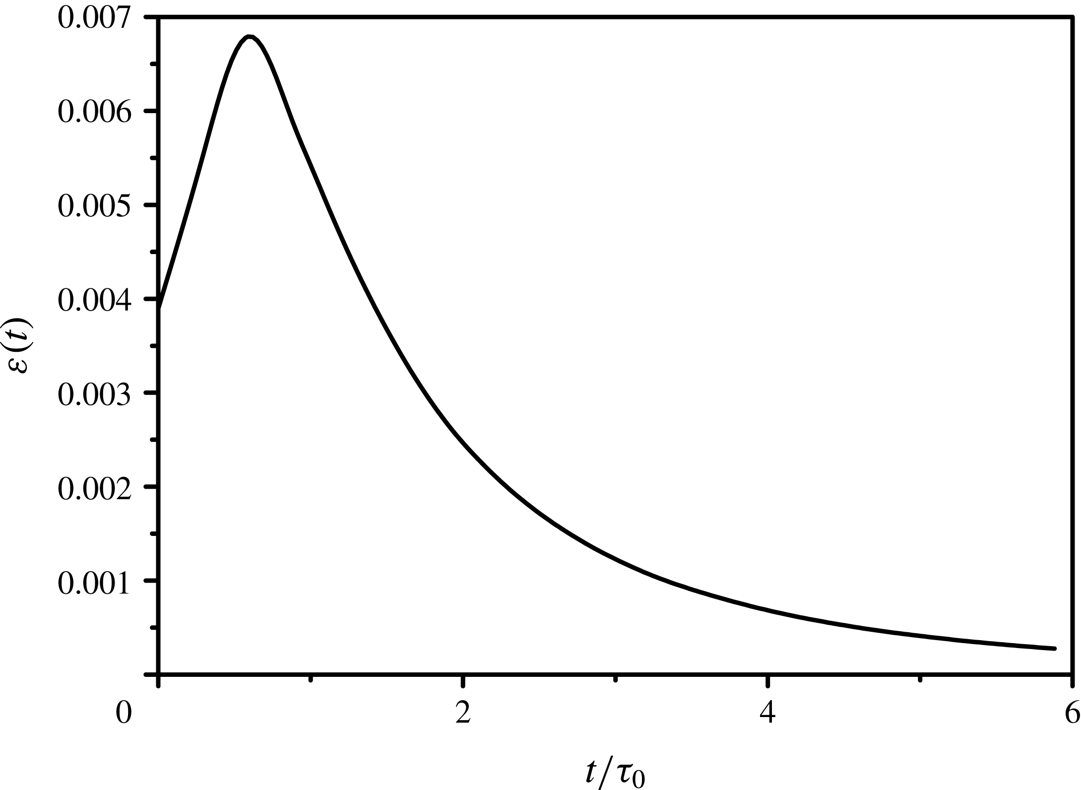
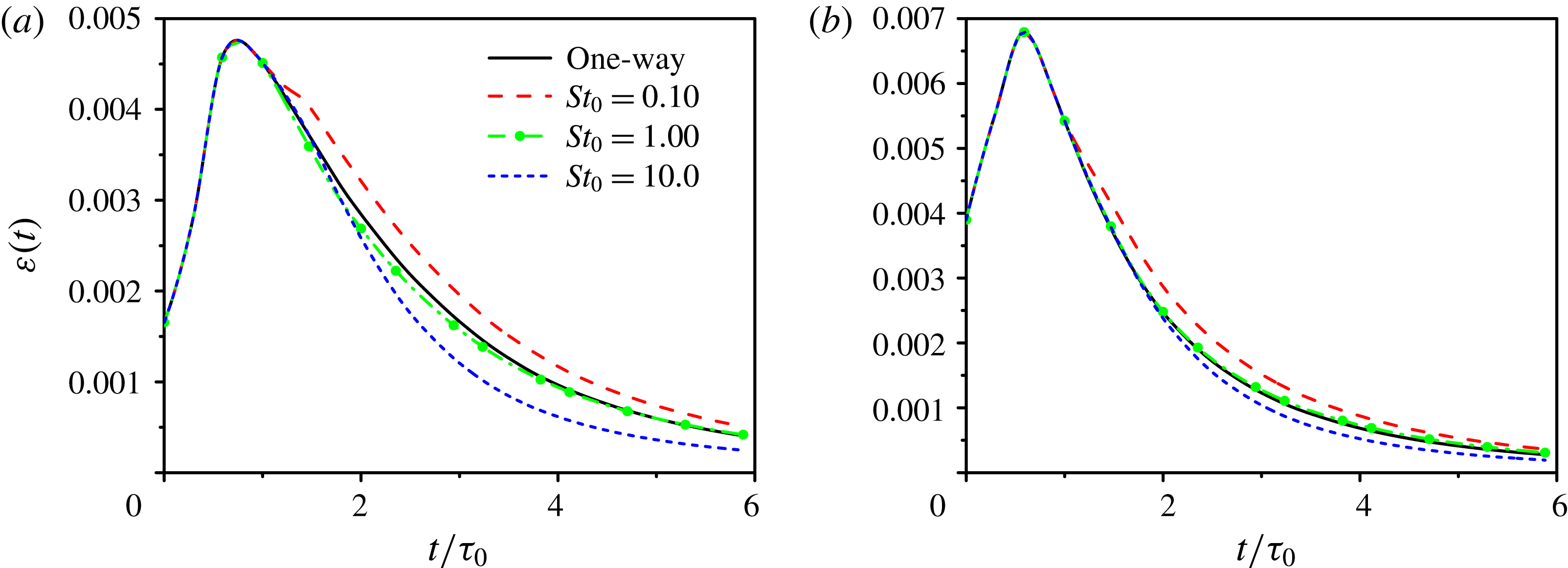
Time development of the energy dissipation rate in the particle-free flow.

The turbulent kinetic energy will decay gradually due to the viscous effect in the present decaying isotropic turbulence. For the energy dissipation, it peaks at the time
 $t\approx 0.6\unicode[STIX]{x1D70F}_{0}$
, as shown in figure 1. Therefore, after an initial large eddy turnover time
 $\unicode[STIX]{x1D70F}_{0}$
, the influence of the initial random field on the flow field has disappeared and turbulence gets fully developed. At this time,
 $N_{p}$
particles are randomly put into the flow field, where particles are uniformly distributed with the same velocity as their surrounding fluid. Periodic boundary conditions are also applied to the particles, which means when a particle leaves the box from one side, it will return to the domain from the opposite side (Mashayek Reference Mashayek1998). The methodology has been validated in our previous works (Jin et al.
Reference Jin, Luo, Dai and Fan2016a
,Reference Jin, Luo, Dai and Fan
b
).
Flow parameters (dimensionless) at initial time (
 $t=0$
), injection time (
 $t=\unicode[STIX]{x1D70F}_{0}$
), and for the particle-free case at time
 $t=4\unicode[STIX]{x1D70F}_{0}$
.

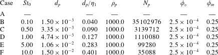
Particle properties (dimensionless) at injection time (
 $t=\unicode[STIX]{x1D70F}_{0}$
).
4 Results and discussions
In the present paper, six cases are simulated to reveal how particles with different diameters (or inertia
 $\unicode[STIX]{x1D70F}_{p}$
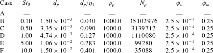
) modify turbulence. The statistics from the particle-free case, which is the same as the one-way coupling flow field, will be used as reference. The flow parameters for reference are shown in table 1, and the particle properties are shown in table 2, where Case A is the particle-free flow and Cases B–F are particle-laden flows with inertia particles of different diameters. The dimensionless density of particles is
 $\unicode[STIX]{x1D70C}_{p}=1000.0$
and the diameters of particles are all smaller than the Kolmogorov length scale. The initial Stokes number is
 $St_{0}=\unicode[STIX]{x1D70F}_{p,0}/\unicode[STIX]{x1D70F}_{\unicode[STIX]{x1D702},1}$
, where
 $\unicode[STIX]{x1D70F}_{p,0}$
is the particle relaxation time and
 $\unicode[STIX]{x1D70F}_{\unicode[STIX]{x1D702},1}$
is the Kolmogorov time scale at the injection time. The volume fraction of particles is
 $\unicode[STIX]{x1D719}_{v}=2.5\times 10^{-4}$
, which is smaller than
 $10^{-3}$
, so the interactions among particles can be neglected and only two-way couplings are considered (Elghobashi Reference Elghobashi1994). The density
 $\unicode[STIX]{x1D70C}_{p}$
and volume fraction of particles
 $\unicode[STIX]{x1D719}_{v}$
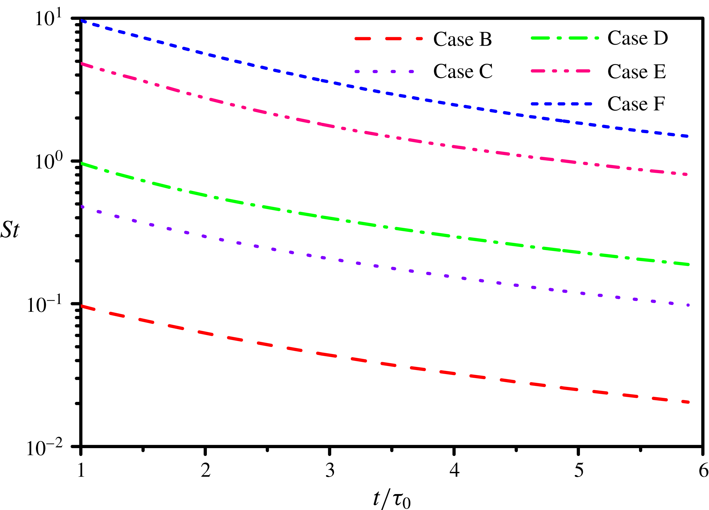
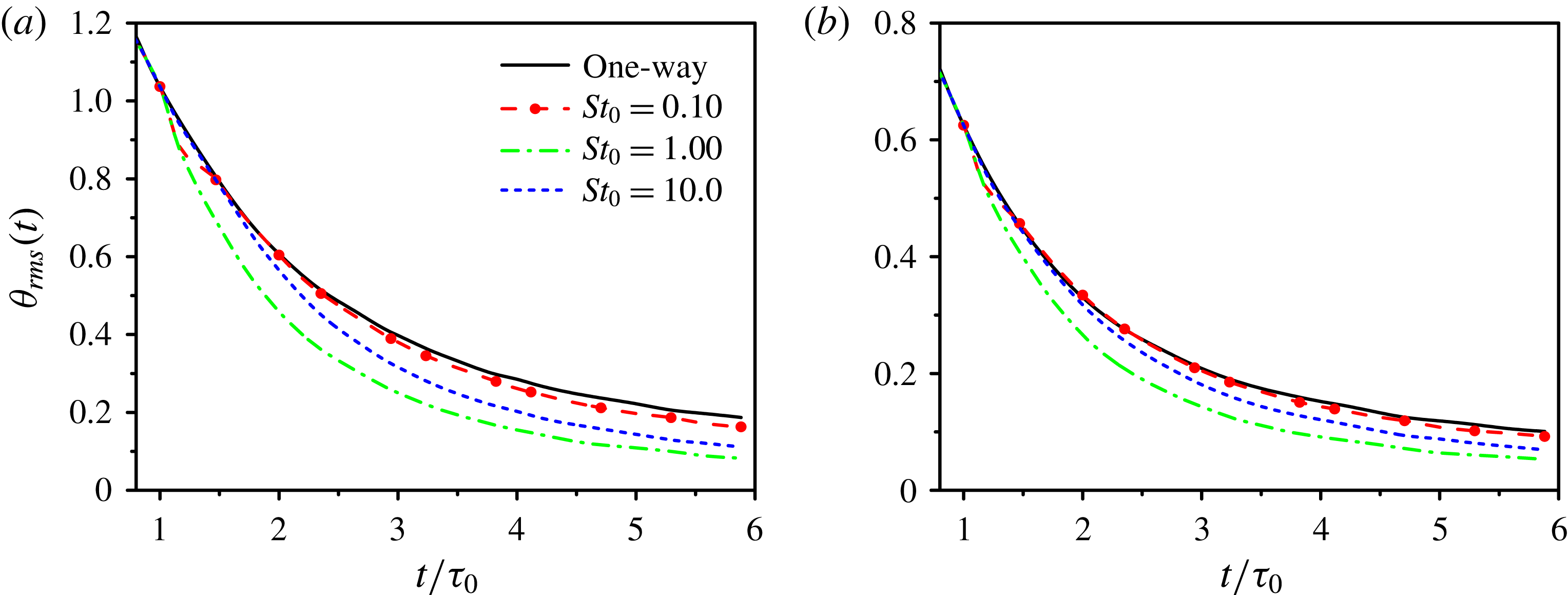
in all five particle-laden cases (B–F) are kept the same. In addition, the temporal evolution of the averaged Stokes numbers of particles is shown in figure 2. The Stokes numbers decrease monotonically to about 20 % level of the initial values by the end of the simulations. As the particle diameters increase, the decay rate of the Stokes numbers increases. Since the decayed kinetic energy will be transformed into the internal energy in compressible turbulence, the dissipation rate is larger and turbulence decays faster compared with incompressible turbulence. Therefore, the increment rate of the Kolmogorov time scale is larger, resulting in larger decay rate of the Stokes numbers than that in incompressible turbulence (Abdelsamie & Lee Reference Abdelsamie and Lee2013).
Here, particles are classified into three categories based on the Stokes number according to Ferrante & Elghobashi (Reference Ferrante and Elghobashi2003): microparticles if
 $St_{0}\leqslant 0.5$
(Case B, C); critical particles if
 $St_{0}\approx 1.0$
(Case D); large particles if
 $St_{0}\geqslant 5.0$
(Case E, F). We study the influence of the particle diameter (or initial Stokes number
 $St_{0}$
) on turbulence through changing the particle number
 $N_{p}$
and the particle diameter
 $d_{p}$
. Since the motions of all kinds of particles can reach the equilibrium with the surrounding fluid after about two large eddy turnover times, which will be shown in § 4.4.1, the statistics of turbulence modulation are mainly investigated after
 $t=3\unicode[STIX]{x1D70F}_{0}$
to avoid the sudden perturbation effect due to the coupling (Abdelsamie & Lee Reference Abdelsamie and Lee2012) and the influence of particle initial conditions.
Time development of the averaged Stokes number of particles.

4.1 Turbulent features of the flow field
In this section, we will investigate the influence of particle diameters on the turbulent features of the flow field, including total energy, turbulent kinetic energy, vorticity magnitude, characteristic length scales and coherent structures.
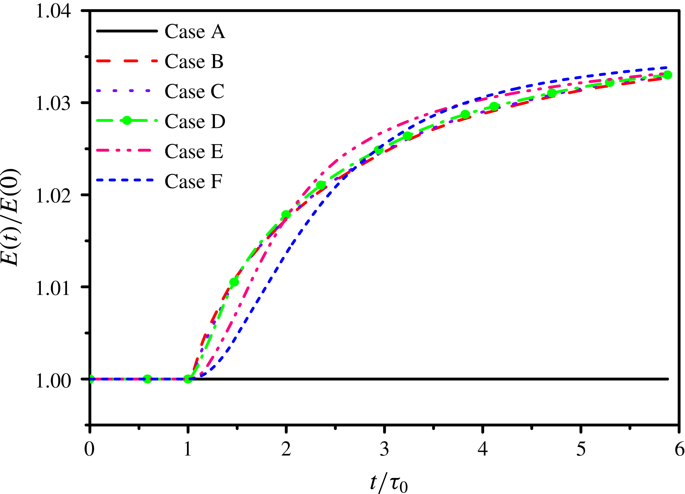
Figure 3 shows the temporal evolution of the total energy normalized by its initial value,
 $E(t)/E(0)$
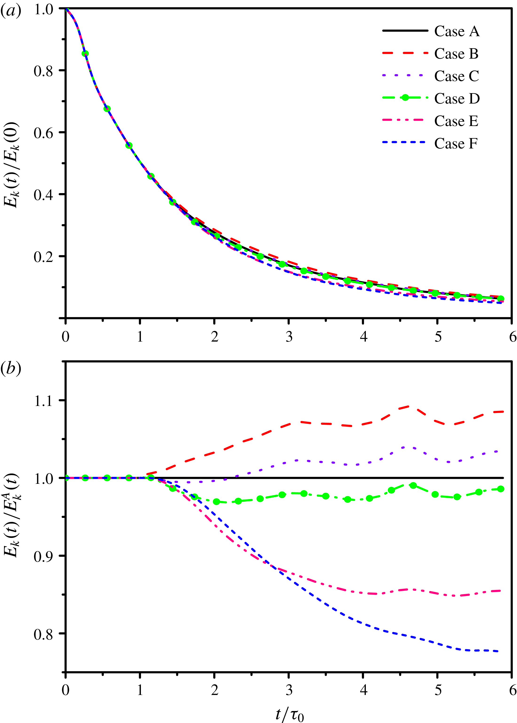
, for all the six cases (A–F). The total energy of the particle-free flow (Case A) is constant, while the addition of particles provides a positive contribution to the turbulence field, causing the enhancement of the total energy. As
 $St_{0}$
increases, the normalized total energy decreases at the time when
 $t\leqslant 1.5\unicode[STIX]{x1D70F}_{0}$
, but increases at the time when
 $t\geqslant 3.5\unicode[STIX]{x1D70F}_{0}$
. Because the fluid velocity is decaying and the density of particles is far larger than that of the fluid, the particle velocity is also decaying but the decay rate is smaller than that of fluid, resulting in the continuous positive work of particles on the fluid and the energy transfer from particles to the turbulence field. As the Stokes number of particles decreases with temporal evolution, the vector alignment between particles and fluid increases (Abdelsamie & Lee Reference Abdelsamie and Lee2013). Thus, the difference between particle and fluid velocity decreases and the increase rate of the total energy is reduced.
Time development of the total energy normalized by its initial value.

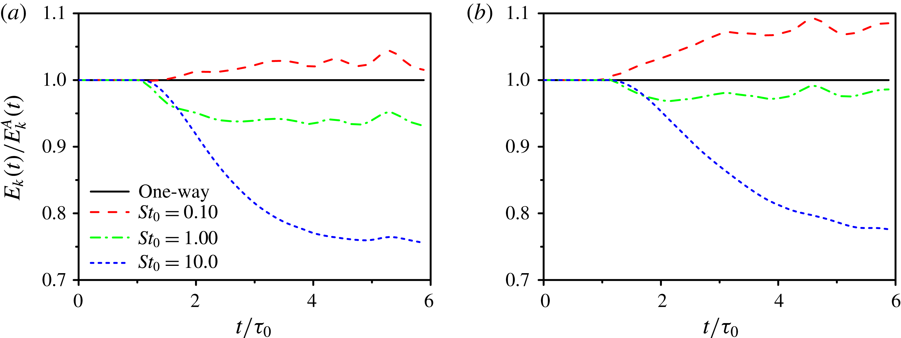
Time development of the turbulent kinetic energy: (a) normalized by its initial value; (b) normalized by the value of the corresponding particle-free case.

Figure 4 shows the temporal evolution of the turbulent kinetic energy (TKE) normalized by its initial value
 $E_{k}(t)/E_{k}(0)$
and the value of the corresponding particle-free case
 $E_{k}(t)/E_{k}^{A}(0)$
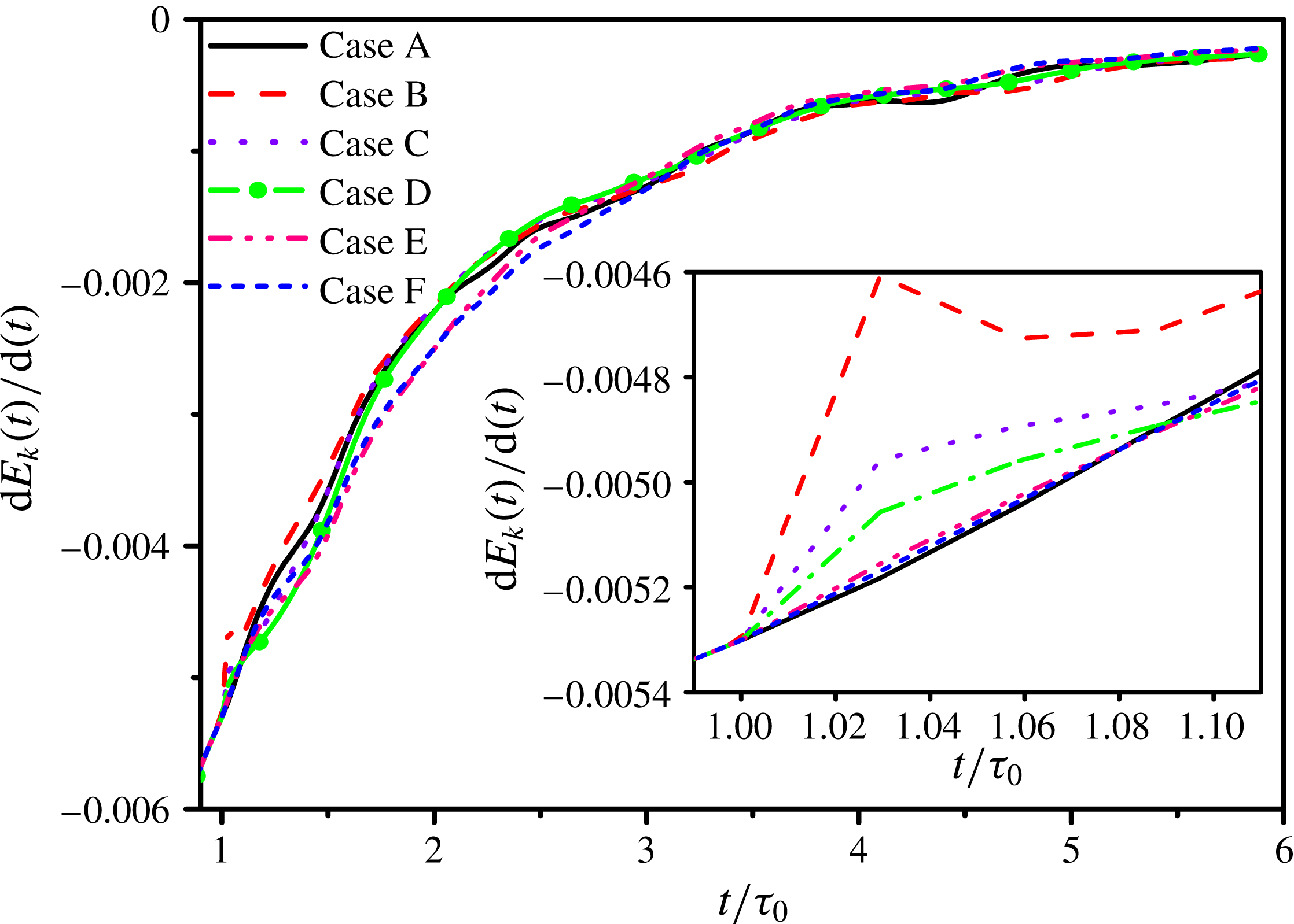
for all the six cases (A–F). Figure 5 displays the time development of the decay rate of TKE
 $\text{d}E_{k}(t)/\text{d}t$
for the same cases. Since TKE of compressible turbulence decays faster than that of incompressible turbulence, the normalized TKE of the particle-laden flows are close to that of the particle-free flow in figure 4(a) although the turbulence modulation by particles is not weak. When the two-way coupling is turned on at
 $t/\unicode[STIX]{x1D70F}_{0}=1$
, the force introduced by the particles suddenly accelerates the fluid (Abdelsamie & Lee Reference Abdelsamie and Lee2012) and the dissipation rate is not modified at that moment, which will be shown in figure 22, resulting in the reduction of the magnitude of
 $\text{d}E_{k}(t)/\text{d}t$
at
 $t/\unicode[STIX]{x1D70F}_{0}=1$
, especially for microparticles (Case B).
Microparticles with
 $St_{0}=0.1$
(Case B) initially reduce the decay rate of TKE, which results in TKE larger than that of the particle-free flow (Case A) at all the times. Microparticles with
 $St_{0}=0.5$
(Case C) initially (
 $1.1\unicode[STIX]{x1D70F}_{0}<t\leqslant 1.5\unicode[STIX]{x1D70F}_{0}$
) slightly enhance the decay rate of TKE and then reduce it, leading to TKE first (
 $\unicode[STIX]{x1D70F}_{0}<t\leqslant 2.2\unicode[STIX]{x1D70F}_{0}$
) smaller and then larger than that of Case A. However, critical and large particles with
 $St_{0}\geqslant 1.0$
(Cases D, E, F) initially enhance the decay rate of TKE, resulting in TKE smaller than that of Case A at all the times. As
 $St_{0}$
increases, TKE decreases at the time when
 $t\geqslant 3\unicode[STIX]{x1D70F}_{0}$
. The modifications are similar to that in decaying incompressible turbulence, where microparticles augment TKE and large particles attenuate TKE (Ferrante & Elghobashi Reference Ferrante and Elghobashi2003; Abdelsamie & Lee Reference Abdelsamie and Lee2012). Nevertheless, they are different from that in forced incompressible and compressible turbulence, where TKE is attenuated by particles for all the cases with
 $0.1\leqslant St_{0}\leqslant 10$
(Boivin et al.
Reference Boivin, Simonin and Squires1998; Xia et al.
Reference Xia, Shi, Zhang and Chen2016). In addition, the normalized TKE and the decay rate of TKE have fluctuations in figures 4(b) and 5 compared with the incompressible flows (Abdelsamie & Lee Reference Abdelsamie and Lee2012), and the amplitude of fluctuation decreases with the increase of particle diameters. Finally at the time
 $t=20$
, compared with TKE in Case A, TKE in Case B is larger by 9 % and TKE in Case E is smaller by 14.5 %, which are larger than 3 % and 12 % in the incompressible cases under the same conditions (He Reference He2004).
Time development of the turbulent kinetic energy decay rate
 $\text{d}Ek(t)/\text{d}t$
.

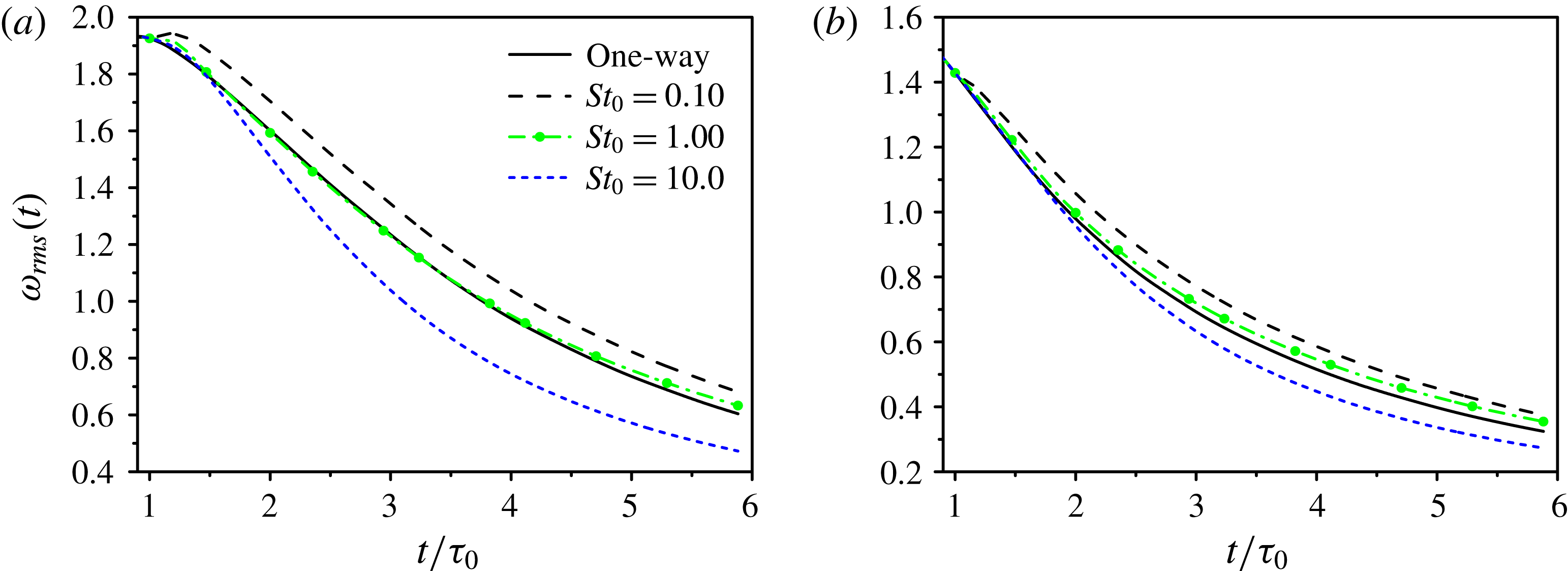
Time development of the r.m.s. of the vorticity magnitude.

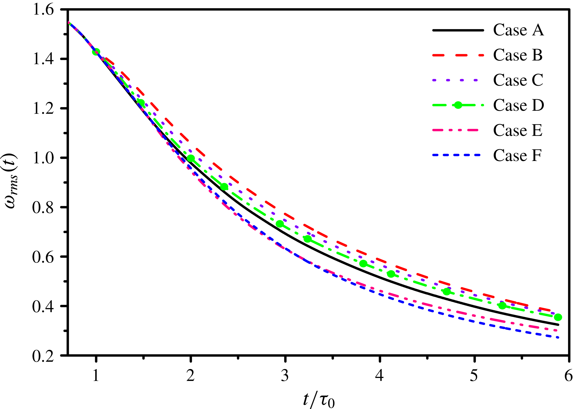
Figure 6 shows the temporal evolution of the r.m.s. of the vorticity magnitude
 $\unicode[STIX]{x1D714}_{rms}$
for all the six cases (A–F). Microparticles and critical particles (Cases B, C, D) enhance the r.m.s. of the vorticity, while large particles (Cases E, F) attenuate the r.m.s. of the vorticity. As
 $St_{0}$
increases,
 $\unicode[STIX]{x1D714}_{rms}$
decreases. Compared with the incompressible turbulence, critical particles (Case D) have more influence on the vorticity in compressible turbulence with a difference 7.7 % at time
 $t=5\unicode[STIX]{x1D70F}_{0}$
, which is larger than 1.4 % at the same time in incompressible turbulence (Ferrante & Elghobashi Reference Ferrante and Elghobashi2003).
Time development of characteristic length scales: (a) the Kolmogorov length scale; (b) the Taylor microscale; (c) the integral length scale.

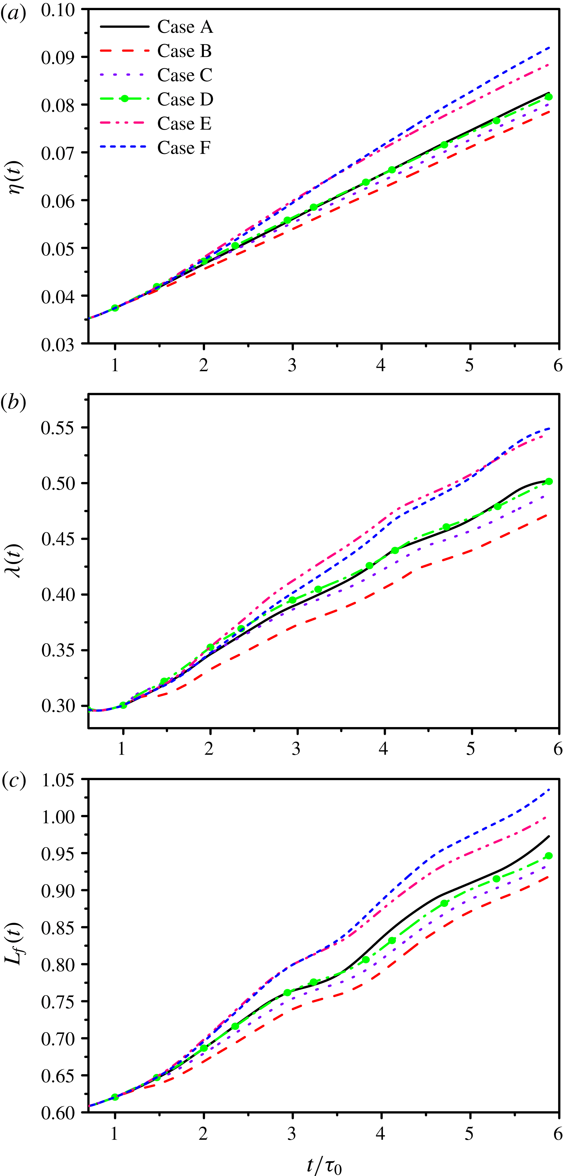
Figure 7 displays the temporal evolution of Kolmogorov length scale
 $\unicode[STIX]{x1D702}$
, Taylor microscale
 $\unicode[STIX]{x1D706}$
and integral length scale
 $L_{f}$
for all the six cases (A–F). Microparticles (Cases B, C) reduce the three characteristic length scales. Critical particles (Case D) hardly modify the three characteristic length scales and make them nearly identical to those of the particle-free flow (Case A) at all the times. Large particles (Cases E, F) enhance the three characteristic length scales. Besides, all the three characteristic length scales increase as
 $St_{0}$
increases.
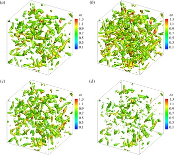
Turbulence vortical structures at time
 $t=4\unicode[STIX]{x1D70F}_{0}$
for different cases: (a) Case A, (b) Case B, (c) Case D and (d) Case F.

Figure 8 shows the distribution of vortical structures in the turbulence field at the time
 $t=4\unicode[STIX]{x1D70F}_{0}$
in the particle-free flow (Case A) and the particle-laden flow (only Cases B, D, F for clarity of the presentation). The vortical structures are identified using the
 $Q$
criterion with
 $Q=0.15$
(Hunt, Wray & Moin Reference Hunt, Wray and Moin1988) and coloured by the local vorticity magnitude
 $\unicode[STIX]{x1D714}$
. The
 $Q$
criterion is the isosurfaces of the second invariant of the instantaneous velocity gradient tensor and given by
 $$\begin{eqnarray}Q=\frac{1}{2}\left(\unicode[STIX]{x1D703}^{2}-s_{ij}s_{ji}+\frac{\unicode[STIX]{x1D714}_{k}^{2}}{2}\right)=\frac{1}{2}\left(\left(\frac{\unicode[STIX]{x2202}u_{i}}{\unicode[STIX]{x2202}x_{i}}\right)^{2}-\frac{\unicode[STIX]{x2202}u_{i}}{\unicode[STIX]{x2202}x_{j}}\frac{\unicode[STIX]{x2202}u_{j}}{\unicode[STIX]{x2202}x_{i}}\right),\end{eqnarray}$$
where
 $s_{ij}=(\unicode[STIX]{x2202}u_{i}/\unicode[STIX]{x2202}x_{j}+\unicode[STIX]{x2202}u_{j}/\unicode[STIX]{x2202}x_{i})/2$
is the strain rate. The particle-free field (Case A) is filled with vermicular vortex tubes. Microparticles with
 $St_{0}=0.1$
(Case B) increase the number of vortex tubes, because their trajectories are almost aligned with the surrounding fluid points’ trajectories and the vorticity of fluid is enhanced. Critical particles with
 $St_{0}=1.0$
weakly influence the vortical structures, because particles mainly accumulate in the peripheries of the vortex cores and the change of the vorticity is relatively small. Large particles with
 $St_{0}=10.0$
(Case F) break the vortex tubes and destroy the coherence of the turbulence field, because they can cross the vortex cores and reduce the vorticity.
4.2 Compressibility of the turbulence field
In this section, we are going to analyse the effect of particles on the compressibility of the turbulence field. In compressible turbulence, the dilatation is not zero and shocklets can exist, which differ from incompressible flows. The dilatation is associated with the fluctuations of thermodynamic quantities (Donzis & Jagannathan Reference Donzis and Jagannathan2013), and thus usually employed to represent the compressibility of the flow field.
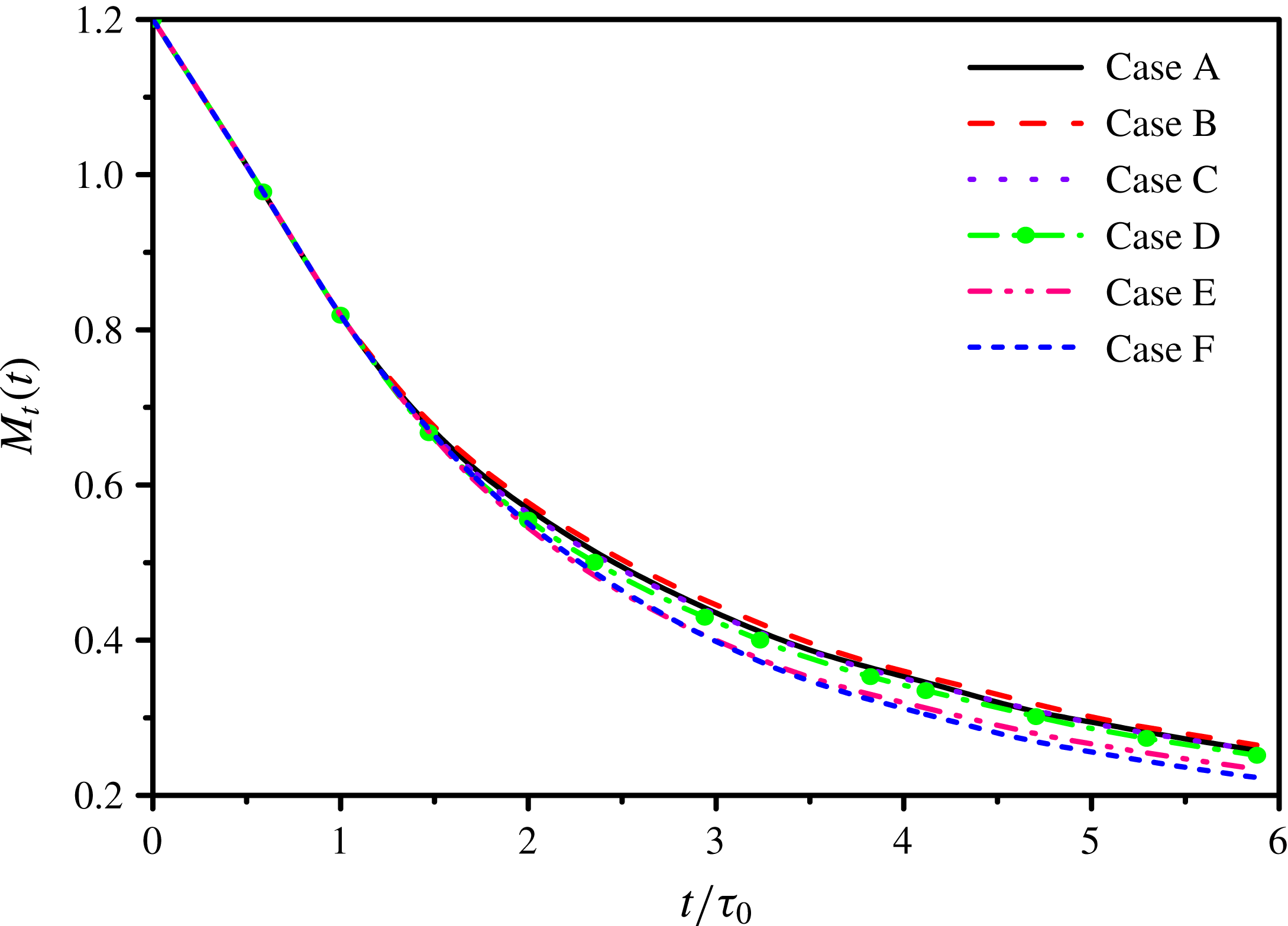
Time development of the turbulent Mach number.

Figure 9 shows the temporal evolution of the turbulent Mach number
 $M_{t}$
for all the six cases (A–F). The decay of
 $M_{t}$
shows that the flow field evolves from the highly compressible turbulence to the weakly compressible turbulence. Microparticles with
 $St_{0}\leqslant 0.5$
(Cases B, C) enhance the turbulent Mach number, while critical and large particles with
 $St_{0}\geqslant 1.0$
(Cases D, E, F) attenuate the turbulent Mach number. These modifications are similar to that of turbulent kinetic energy in figure 4.
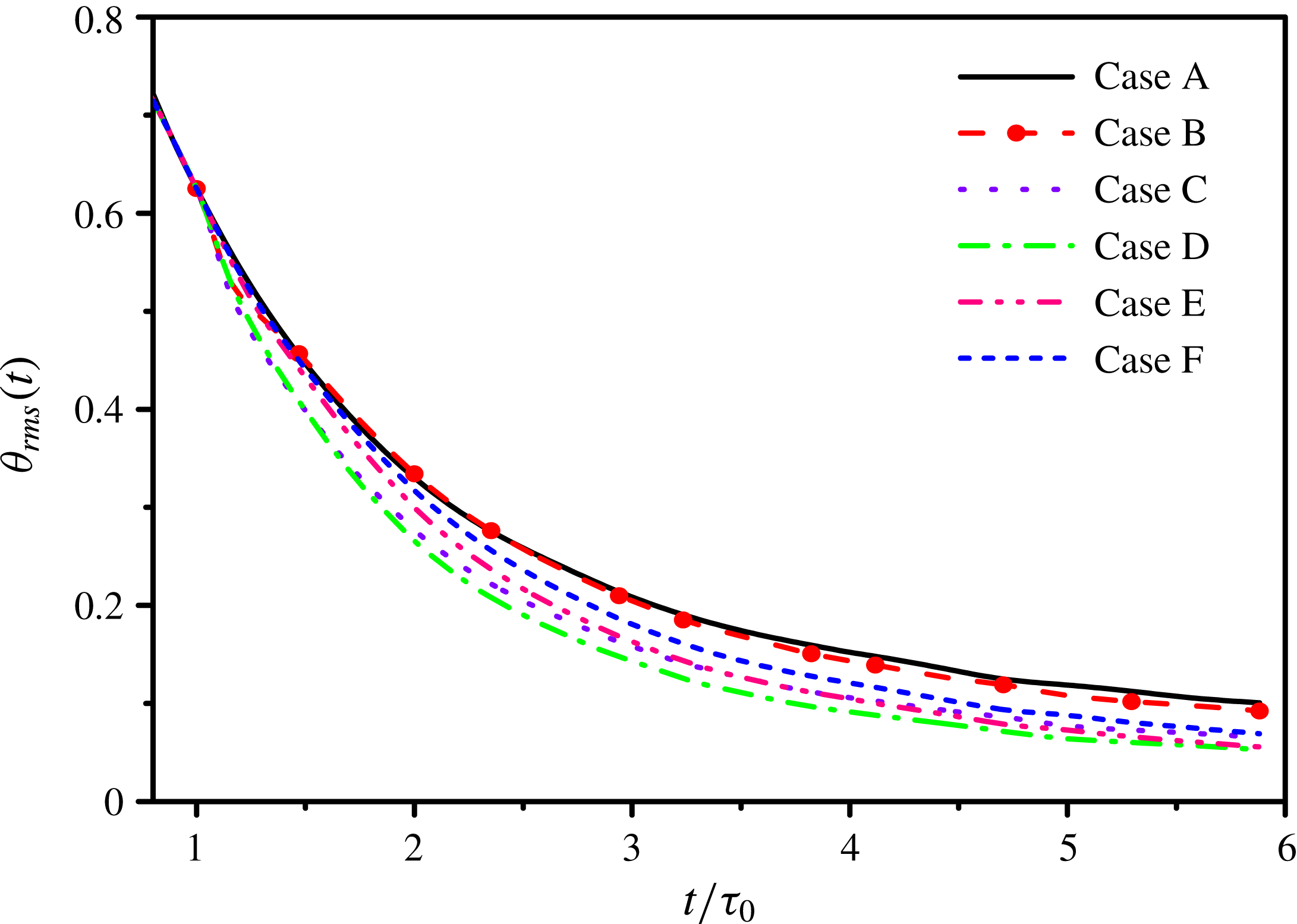
Time development of the r.m.s. of the dilatation.

Figure 10 shows the temporal evolution of the r.m.s. of the dilatation
 $\unicode[STIX]{x1D703}_{rms}$
for all the six cases (A–F). The addition of particles reduces the r.m.s. of the dilatation compared with the particle-free flow (Case A), which means the compressibility of the turbulence field is attenuated.
 $\unicode[STIX]{x1D703}_{rms}$
first decreases and then increases with the increment of
 $St_{0}$
, and
 $\unicode[STIX]{x1D703}_{rms}$
is the smallest in Case D (critical particles with
 $St_{0}=1.0$
) compared with the other cases.
According to Samtaney et al. (Reference Samtaney, Pullin and Kosović2001), the shocklets of compressible isotropic turbulence are a set of disjoint surfaces, where the compression rate is high and the local density exhibits inflection along the normal direction. Each surface may be simply or multiply connected, which is defined as
 $$\begin{eqnarray}S=\{S_{l}|\unicode[STIX]{x1D6FB}^{2}\unicode[STIX]{x1D70C}=0,\unicode[STIX]{x1D703}<-3\unicode[STIX]{x1D703}_{rms}\}.\end{eqnarray}$$
Therefore, the shocklets are identified by the isosurfaces of
 $\unicode[STIX]{x1D703}=-3\unicode[STIX]{x1D703}_{rms}$
(Wang et al.
Reference Wang, Shi, Wang, Xiao, He and Chen2012a
). For the clarity of the presentation, the results only from Cases A, B, D and F are shown.
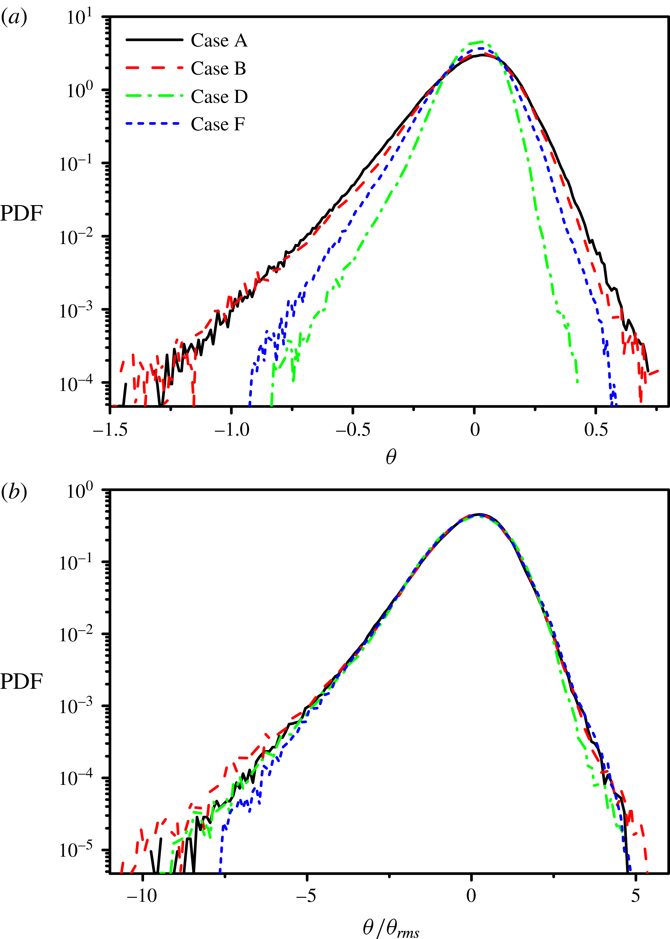
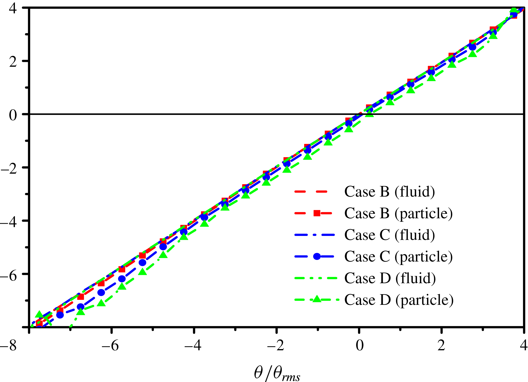
Probability density functions (PDF) of (a) velocity divergence; (b) normalized velocity divergence at time
 $t=4\unicode[STIX]{x1D70F}_{0}$
.

Figure 11 provides the probability density functions (PDFs) of the velocity divergence
 $\unicode[STIX]{x1D703}$
and the normalized velocity divergence
 $\unicode[STIX]{x1D703}/\unicode[STIX]{x1D703}_{rms}$
at time
 $t=4\unicode[STIX]{x1D70F}_{0}$
. The addition of particles attenuates the fluctuations of dilatation and the attenuation becomes more significant if
 $St_{0}$
gets close to 1. In addition, there is a strong tendency for the PDFs of the velocity divergence to be skewed to the negative value: the right tail of the PDFs falls fast, while the left tail is very long (Wang et al.
Reference Wang, Shi, Wang, Xiao, He and Chen2012a
). Microparticles with
 $St_{0}=0.1$
(Case B) augment the skewness which makes the left tail longer; critical particles with
 $St_{0}=1.0$
(Case D) hardly change the skewness although the velocity divergence is reduced; large particles with
 $St_{0}=10.0$
(Case F) attenuate the skewness and shorten the left tail.
Shocklet structures at time
 $t=4\unicode[STIX]{x1D70F}_{0}$
for different cases: (a) Case A, (b) Case B, (c) Case D and (d) Case F.

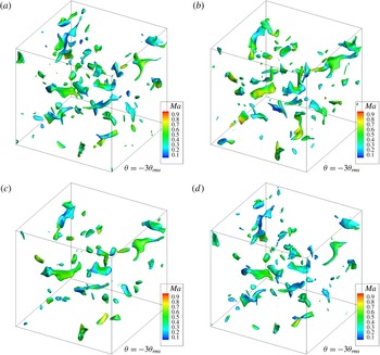
Figure 12 shows the shocklet structures coloured by the local Mach number at the same time
 $t=4\unicode[STIX]{x1D70F}_{0}$
. Blob-like shocklet structures are sparsely distributed in the particle-free turbulence field (Case A), which is similar to the findings of Wang, Gotoh & Watanabe (Reference Wang, Gotoh and Watanabe2017a
). Microparticles (Case B) hardly change the structures of isosurfaces. Critical particles (Case D) enlarge the area of isosurfaces and reduce the number of isosurfaces, illustrating that the compressibility of the turbulence field is attenuated. Large particles (Case F) make the isosurfaces more scattered, which means the destruction of the coherence.
4.3 Energy spectra of the turbulence field
Turbulent kinetic energy is the integral of the three-dimensional density-weighted kinetic energy spectra
 $E_{\unicode[STIX]{x1D70C}}(k)=\sum _{k\leqslant |\boldsymbol{k}|<k+1}|\hat{\boldsymbol{w}}(\boldsymbol{k})|^{2}/2$
(where
 $\hat{\boldsymbol{w}}=\widehat{\unicode[STIX]{x1D70C}^{0.5}\boldsymbol{u}}$
) at all scales of the turbulence field (Wang et al.
Reference Wang, Yang, Shi, Xiao, He and Chen2013). As the density of fluid points varies with locations and time in compressible turbulence, the density-weighted kinetic energy spectra of the turbulence field will be investigated in this section.
Density-weighted kinetic energy spectra
 $E_{\unicode[STIX]{x1D70C}}(k)$
at time
 $t=4\unicode[STIX]{x1D70F}_{0}$
.

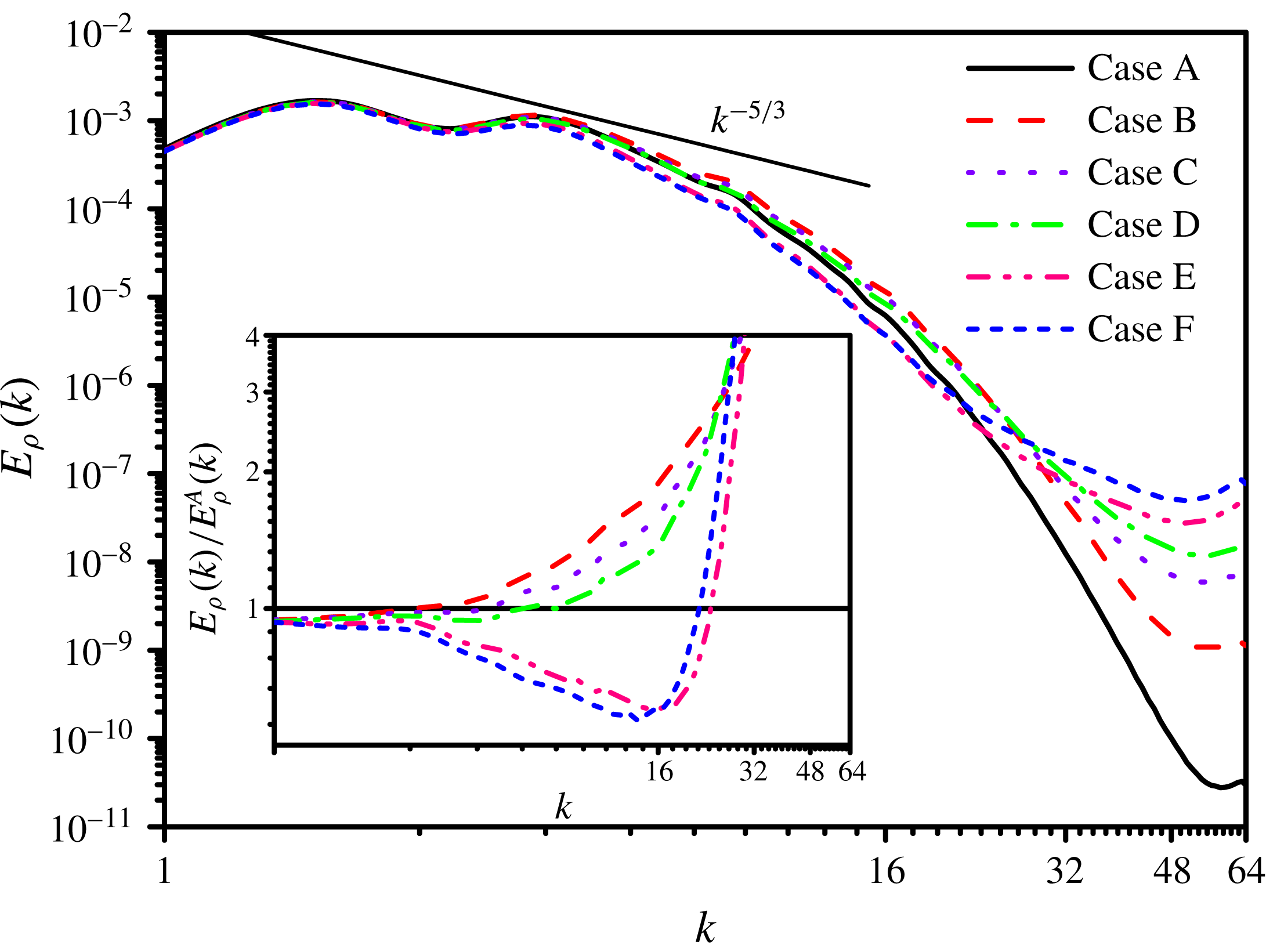
Figure 13 shows the density-weighted kinetic energy spectra
 $E_{\unicode[STIX]{x1D70C}}(k)$
at time
 $t=4\unicode[STIX]{x1D70F}_{0}$
for all the six cases (A–F). The energy spectra exhibits attenuation at low wavenumbers (large eddies) and augmentation at high wavenumbers (small eddies) in the particle-laden flow compared with the particle-free flow, which is similar to incompressible turbulence (Boivin et al.
Reference Boivin, Simonin and Squires1998; Ferrante & Elghobashi Reference Ferrante and Elghobashi2003). For the medium wavenumbers (intermediate eddies), the energy spectra are augmented by microparticles and critical particles with
 $St_{0}\leqslant 1.0$
(Cases B, C and D), and attenuated by large particles with
 $St_{0}\geqslant 5.0$
(Cases E and F). As the particles’ diameter increases, the small eddy energy increases but the energy of intermediate eddies and large eddies decreases, which is different from some researches in incompressible turbulence (Ferrante & Elghobashi Reference Ferrante and Elghobashi2003; Abdelsamie & Lee Reference Abdelsamie and Lee2012), where the energy of small eddies, intermediate eddies and large eddies all decreases with the increase of the particles’ diameter.
Microparticles with
 $St_{0}=0.1$
(Case B) increase
 $E_{\unicode[STIX]{x1D70C}}(k)$
at wavenumbers
 $k\geqslant 3$
, and reduce
 $E_{\unicode[STIX]{x1D70C}}(k)$
only at wavenumbers
 $k=1$
and 2; critical particles with
 $St_{0}=1.0$
(Case D) increase
 $E_{\unicode[STIX]{x1D70C}}(k)$
at wavenumbers
 $k\geqslant 6$
, and reduce
 $E_{\unicode[STIX]{x1D70C}}(k)$
at wavenumbers
 $k\leqslant 5$
; large particles with
 $St_{0}=10.0$
(Case F) increase
 $E_{\unicode[STIX]{x1D70C}}(k)$
at wavenumbers
 $k\geqslant 22$
, and reduce
 $E_{\unicode[STIX]{x1D70C}}(k)$
at wavenumbers
 $k\leqslant 21$
. At the increase of
 $St_{0}$
, the crossing point of
 $E_{\unicode[STIX]{x1D70C}}(k)$
between the two-way coupled simulation and the one-way coupled simulation (the domain where the energy spectrum is attenuated) shifts to the right (toward high wavenumbers), which nevertheless appears at the wavenumber lower than that of the forced compressible turbulence (Xia et al.
Reference Xia, Shi, Zhang and Chen2016). In Cases B and C (
 $St_{0}\leqslant 0.5$
), the reduction at low wavenumbers is less than the augment at high wavenumbers, resulting in the enhancement of TKE. However, in Cases D, E and F (
 $St_{0}\geqslant 1.0$
), the reduction at low wavenumbers surpasses the augment at high wavenumbers, leading to the attenuation of TKE, as shown in figure 4.
In order to further understand the modification of
 $E_{\unicode[STIX]{x1D70C}}(k)$
, the evolution equation for the density-weighted kinetic energy spectrum (Xia et al.
Reference Xia, Shi, Zhang and Chen2016) is investigated,
 $$\begin{eqnarray}\frac{\unicode[STIX]{x2202}E_{\unicode[STIX]{x1D70C}}(k)}{\unicode[STIX]{x2202}t}=T(k)+P(k)-D(k)+F(k),\end{eqnarray}$$
where
 $T(k)$
is the spectral nonlinear energy transfer rate due to the convection,
 $P(k)$
is the spectral energy transfer rate due to the pressure gradient and
 $D(k)$
is the spectral viscous dissipation rate.
 $F(k)$
is the spectral two-way interaction energy rate, which can be expressed as
 $$\begin{eqnarray}F(k)=\mathop{\sum }_{k\leqslant |\boldsymbol{k}|<k+1}\text{Re}\left\{{\hat{w}}_{i}^{\ast }(\boldsymbol{k})\widehat{\frac{\unicode[STIX]{x1D711}_{ui}}{\unicode[STIX]{x1D70C}^{0.5}}}(\boldsymbol{k})\right\},\end{eqnarray}$$
where ‘
 $\hat{~}$
’ denotes the Fourier transform, ‘
 $\text{}^{\ast }$
’ denotes the complex conjugate and
 $\text{Re}\{~\}$
denotes the real part.
(a) Spectral nonlinear energy transfer rate due to the convection
 $T(k)$
; (b) spectral energy transfer rate due to the pressure gradient
 $P(k)$
;(c) the opposite of viscous dissipation rate spectrum
 $D(k)$
; (d) two-way interaction energy rate spectrum
 $F(k)$
at time
 $t=4\unicode[STIX]{x1D70F}_{0}$
.

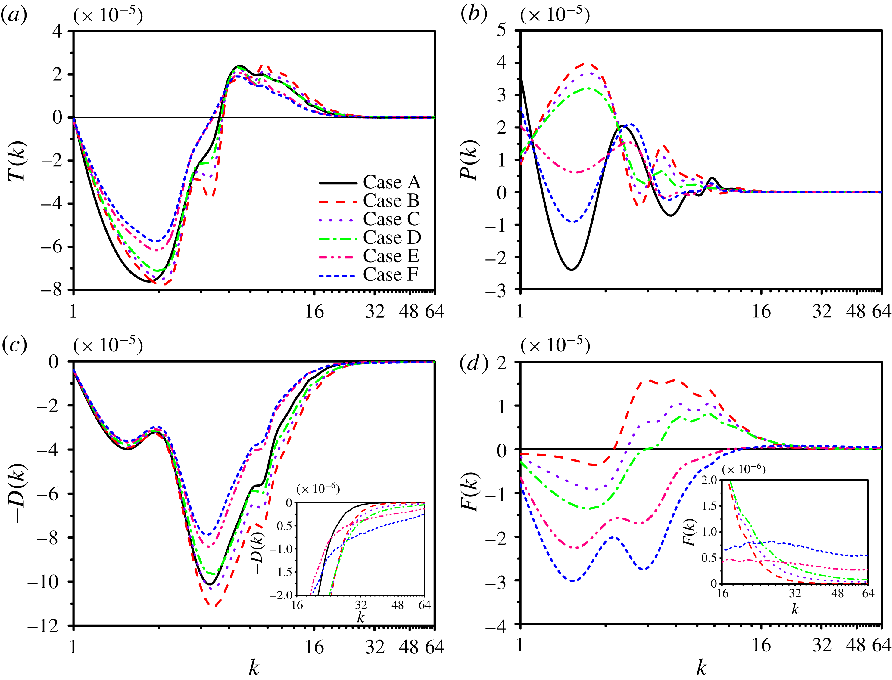
Figure 14 shows the spectral nonlinear energy transfer rate due to the convection, the spectral energy transfer rate due to the pressure gradient, the viscous dissipation rate spectrum and the two-way interaction energy rate spectrum at time
 $t=4\unicode[STIX]{x1D70F}_{0}$
for all the six cases (A–F).
 $P(k)$
oscillates sharply around 0 at low wavenumbers, but the magnitude of oscillations decreases with the increment of wavenumbers, resulting in the slight fluctuation of energy spectra at low wavenumbers. Nevertheless, the influence of the integral of
 $P(k)$
on the averaged turbulent kinetic energy is negligible (Wang et al.
Reference Wang, Shi, Wang, Xiao, He and Chen2012a
).
The ratio of the particle energy spectrum
 $E_{vv}(k)$
to the fluid energy spectrum along the particle trajectory
 $E_{uu}(k)$
at time
 $t=4\unicode[STIX]{x1D70F}_{0}$
.

The two-way interaction energy rate spectrum
 $F(k)$
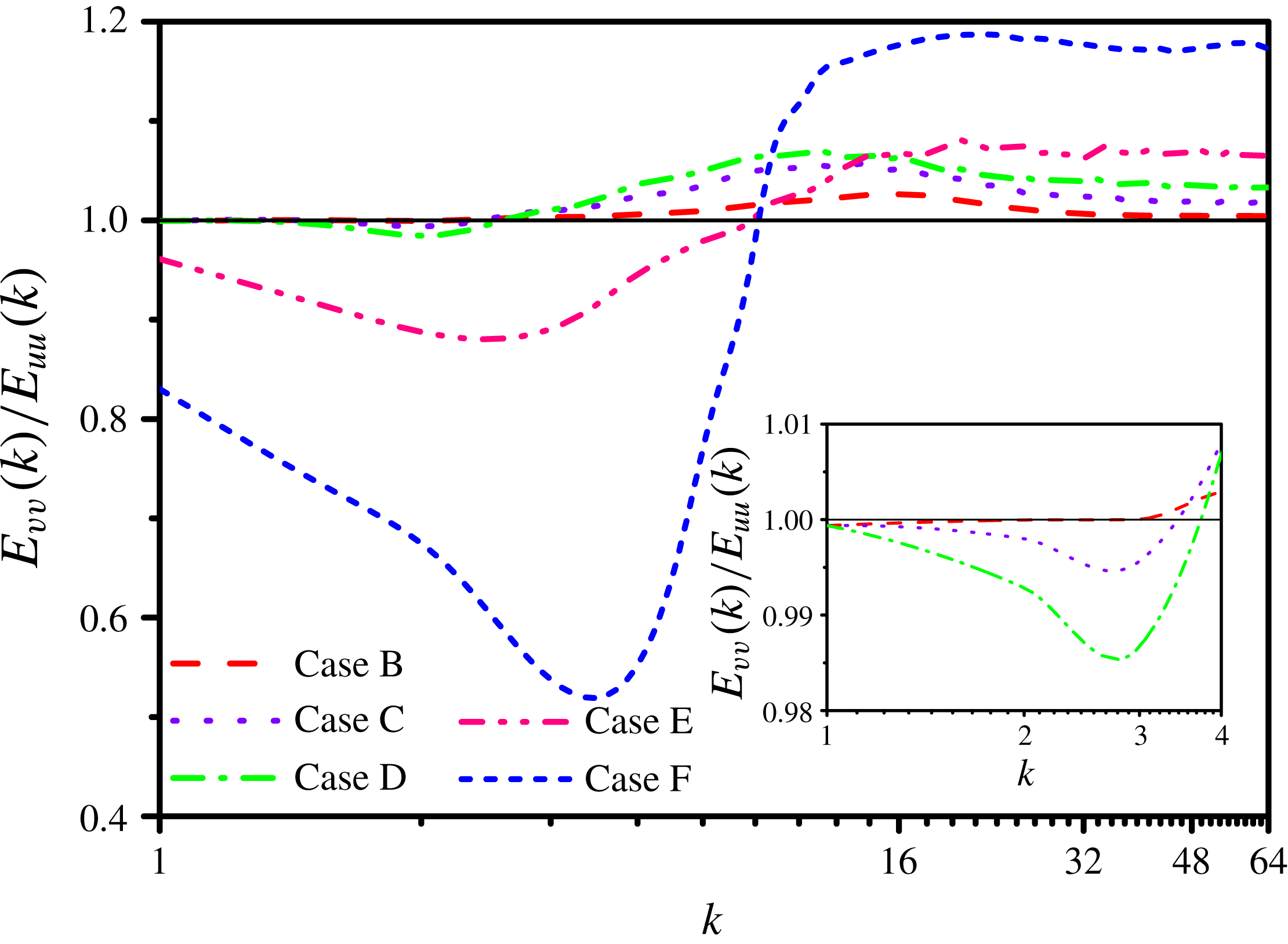
is positive at high wavenumbers because the particle velocity is larger than the fluid velocity of small eddies, as shown in figure 15. In addition, the transfer of the fluid–particle covariance by the fluid turbulence also contribute to
 $F(k)$
positive at high wavenumbers (Boivin et al.
Reference Boivin, Simonin and Squires1998). Therefore, the drag force of particles represents a source to the energy of small eddies. As the diameters of particles are smaller than the Kolmogorov length scale and the Stokes numbers of particles decrease faster compared with incompressible turbulence, particles directly interact with small eddies and have stronger tendency to follow the trajectories of fluid points in small eddies of compressible turbulence. With the increment of
 $St_{0}$
, the difference between particle velocity and fluid velocity increase and particles provide a larger two-way interaction contribution in compressible turbulence. Hence, the magnitude of
 $F(k)$
at high wavenumbers increases with
 $St_{0}$
as shown in figure 14(d), which is contrary to that in the incompressible turbulence (Ferrante & Elghobashi Reference Ferrante and Elghobashi2003; Abdelsamie & Lee Reference Abdelsamie and Lee2012). Accordingly, the energy of small eddies increases with the particles’ diameter.
Due to the non-local triadic interactions among different wavenumbers, the addition of particles also modifies the energy of eddies with the other scales (Xia et al. Reference Xia, Shi, Zhang and Chen2016).
Since the particle velocity is smaller than the fluid velocity of large eddies, negative regions of
 $F(k)$
appear at low wavenumbers and their magnitude increase with
 $St_{0}$
, which is the same as that in incompressible turbulence (Ferrante & Elghobashi Reference Ferrante and Elghobashi2003; Abdelsamie & Lee Reference Abdelsamie and Lee2012).
For Cases B and C,
 $F(k)$
is slightly negative at low wavenumbers and positive at medium–high wavenumbers. Therefore, the drag force of microparticles represents a source to energy spectrum. Furthermore,
 $D(k)$
is enhanced at medium–high wavenumbers. Due to the increase of dissipation at high wavenumbers, the energy transfer rate from large eddies to small eddies is also augmented as shown in figure 14(a), where the
 $k$
at which
 $T(k)=0$
is shifted towards higher wavenumbers compared with Case A. Thus, the energy of large eddies is attenuated.
For Case D,
 $F(k)$
is negative at low wavenumbers and positive at high wavenumbers. However,
 $D(k)$
and
 $T(k)$
are hardly altered at all the wavenumbers. Therefore, the energy of large eddies is attenuated.
For Cases E and F,
 $F(k)$
is negative at low wavenumbers and slightly positive at high wavenumbers. Thus, large particles provide a negative two-way interaction contribution to energy spectrum. Besides,
 $D(k)$
is reduced at nearly all wavenumbers except for slight enhancement at high wavenumbers. Since the whole dissipation at medium–high wavenumbers is attenuated, the
 $k$
at which
 $T(k)=0$
is shifted towards smaller wavenumbers compared with Case A in figure 14(a) and the energy transfer rate from large eddies to small eddies is also reduced. Nevertheless, the reduction of
 $D(k)$
and
 $T(k)$
at low wavenumbers is smaller than
 $F(k)$
, resulting in the attenuation of the large eddy energy.
At medium wavenumbers,
 $F(k)$
is positive for Cases B, C and D, but negative for Cases E and F as the fluid velocity of intermediate eddies is smaller than the velocity of microparticles and critical particles, and larger than the velocity of large particles. With the increment of the particles’ diameter, the particles’ trajectories are less aligned with fluid points’ trajectories, which in turn reduce the fluid–particle covariance transfer. Therefore, the
 $k$
at which
 $E_{vv}(k)/E_{uu}(k)=1$
is shifted towards higher wavenumbers and the wavenumber range of the positive regions of
 $F(k)$
decrease as the particles’ diameter increase. Consequently, the intermediate eddy energy is augmented by microparticles and critical particles, but attenuated by large particles.
4.4 Mechanisms of turbulence modulation by particles
In this section, we will describe in detail the underlying mechanisms responsible for the modifications of decaying compressible isotropic turbulence by particles, including turbulent kinetic energy, the rotational motion (or the vorticity) and the compressibility (or the dilatation). For the clarity of the presentation, the mechanisms of turbulence modulation in only three cases are shown, which are Case B (microparticles with
 $St_{0}=0.1$
), Case D (critical particles with
 $St_{0}=1.0$
) and Case F (large particles with
 $St_{0}=10.0$
).
4.4.1 Evolution of particle distributions in the turbulence field
It is necessary to first investigate the spatial distributions of particles in the turbulence field, as the local concentration of particles is highly related to the structures of the surrounding flow (Maxey Reference Maxey1987).
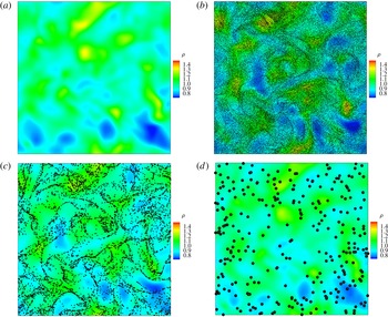
Superimposed particles on density contours at
 $x_{1}=\unicode[STIX]{x1D70B}$
and
 $t=4\unicode[STIX]{x1D70F}_{0}$
in different cases: (a) Case A, (b) Case B, (c) Case D and (d) Case F.

Figure 16 shows the contours of density
 $\unicode[STIX]{x1D70C}$
with superimposed particles at
 $x_{1}=\unicode[STIX]{x03C0}$
and
 $t=4\unicode[STIX]{x1D70F}_{0}$
in different cases. Particles have the tendency to accumulate in high-density regions, which is attributed to two reasons (Zhang et al.
Reference Zhang, Liu, Ma and Xiao2016). One is the centrifugal effect that particles tend to accumulate in the low-vorticity regions corresponding to the regions with high density, because of the negative correlation between local fluid density and vorticity in the regions without shocklets. The other is the compressive property of the turbulence field that particles would like to accumulate in the downstream regions of shocklets with high fluid density. In addition, the tendency of preferential accumulation in high-density regions is strongest for critical particles (Case D) and weakest for large particles (Case F).
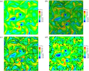
Superimposed particles on the contours of normalized vorticity in
 $x_{1}$
direction at
 $x_{1}=\unicode[STIX]{x1D70B}$
and
 $t=4\unicode[STIX]{x1D70F}_{0}$
in different cases: (a) Case A, (b) Case B, (c) Case D and (d) Case F.
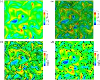
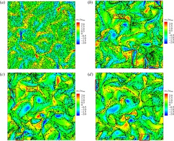
Superimposed particles on the contours of normalized vorticity in
 $x_{1}$
direction at
 $x_{1}=\unicode[STIX]{x1D70B}$
in Case D for different time: (a)
 $t=\unicode[STIX]{x1D70F}_{0}$
, (b)
 $t=2\unicode[STIX]{x1D70F}_{0}$
, (c)
 $t=3\unicode[STIX]{x1D70F}_{0}$
and (d)
 $t=4\unicode[STIX]{x1D70F}_{0}$
.

Figure 17 shows the contours of normalized vorticity
 $\unicode[STIX]{x1D714}_{1}/\unicode[STIX]{x1D714}_{rms}$
with superimposed particles at
 $x_{1}=\unicode[STIX]{x03C0}$
and
 $t=4\unicode[STIX]{x1D70F}_{0}$
in different cases, and figure 18 shows superimposed particles on the contours of
 $\unicode[STIX]{x1D714}_{1}/\unicode[STIX]{x1D714}_{rms}$
at
 $x_{1}=\unicode[STIX]{x03C0}$
in Case D for different time. Particles tend to cluster in the regions of low vorticity, and critical particles (Case D) show the maximum preferential accumulation compared with the other cases. Microparticles (Case B) respond fast to the fluid motion and follow the streamline of fluid points, as the particle relaxation time is much smaller than the Kolmogorov time scale. Thus, most microparticles are not ejected out of the vortical structures but rather trapped in the vortex cores. Large particles (Case F) respond slowly to the fluid motion because of the high particle relaxation time which is larger than the Kolmogorov time scale. Therefore, large particles move randomly independent of the surrounding fluid motion, and cross the trajectories of the fluid points. Critical particles (Case D) are ejected out of the vortex cores with high vorticity, and accumulate in the peripheries of the vortical structures with low vorticity, rather than moving as the fluid points’ trajectories like microparticles or randomly like large particles. In this regard, the tendency that critical particles mostly cluster in the low-vorticity regions is similar to that in incompressible flows. On the other hand, at the initial time when the turbulent Mach number is high, some of critical particles also have the tendency to collect in the high-vorticity regions, as shown in the red frames of figure 18. As the increase of time, such tendency become weak due to the decay of the compressibility. This evolution is attributed to the interaction between particles and shocklets that particles would like to accumulate in the downstream regions of shocklets with both high fluid density and high vorticity (Yang et al.
Reference Yang, Wang, Shi, Xiao, He and Chen2014). When turbulent Mach number decreases, the tendency that critical particles prefer to accumulate in the high-vorticity regions becomes weak. Nevertheless, these regions only take up a very small fraction of the flow field, which is less than 0.4 % (Zhang et al.
Reference Zhang, Liu, Ma and Xiao2016).
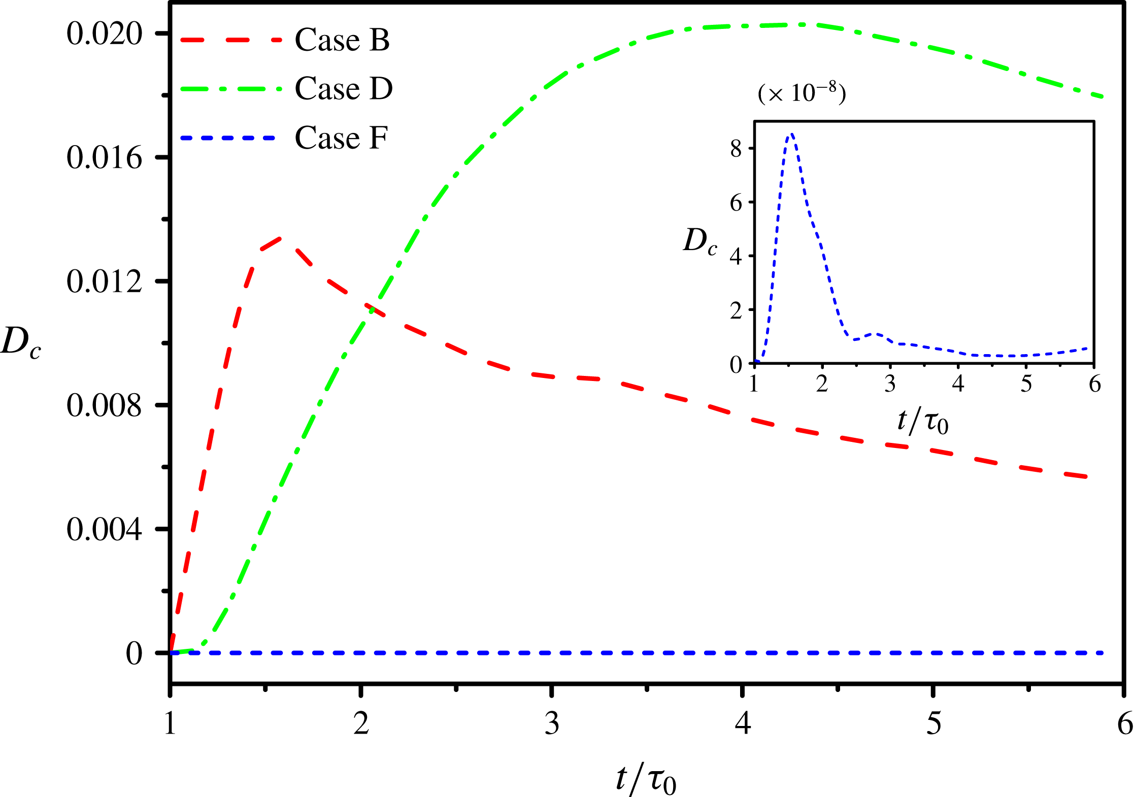
To accomplish the quantitative analysis of preferential accumulation, the temporal evolution of the
 $D_{c}$
factor is investigated (Ferrante & Elghobashi Reference Ferrante and Elghobashi2003), which reflects the difference between the actual distribution and the uniform distribution of particles,
 $$\begin{eqnarray}D_{c}=\mathop{\sum }_{C=0}^{N_{p}}(P_{c}(C)-P_{c}^{\unicode[STIX]{x1D707}}(C))^{2},\end{eqnarray}$$
where the actual distribution probability function
 $P_{c}(C)$
is the probability of finding particles whose number is
 $C$
in one grid. The uniform distribution probability function
 $P_{c}^{\unicode[STIX]{x1D707}}(C)$
is calculated from
 $$\begin{eqnarray}P_{c}^{\unicode[STIX]{x1D707}}(C)=\left(\begin{array}{@{}l@{}}N_{P}\\ C\end{array}\right)\left(\frac{1}{N_{g}}\right)^{C}\left(1-\frac{1}{N_{g}}\right)^{N_{P}-C},\quad C=1,2,\ldots ,N_{P},\end{eqnarray}$$
where
 $N_{g}=128^{3}$
is the number of grid points, and
 $$\begin{eqnarray}\left(\begin{array}{@{}l@{}}N_{p}\\ C\end{array}\right)=\frac{N_{P}(N_{P}-1)\ldots (N_{P}-C+1)}{C!}.\end{eqnarray}$$
Figure 19 shows the temporal evolution of the
 $D_{c}$
factor for Cases B, D and F. It is clear that critical particles (Case D) have the strongest preferential concentration, while large particles (Case F) have the weakest preferential concentration. At the initial time after particles are injected, microparticles (Case B) and large particles have relatively stronger preferential concentration. Then, the preferential concentration is attenuated with the decay of turbulence.
Time development of the
 $D_{c}$
factor.

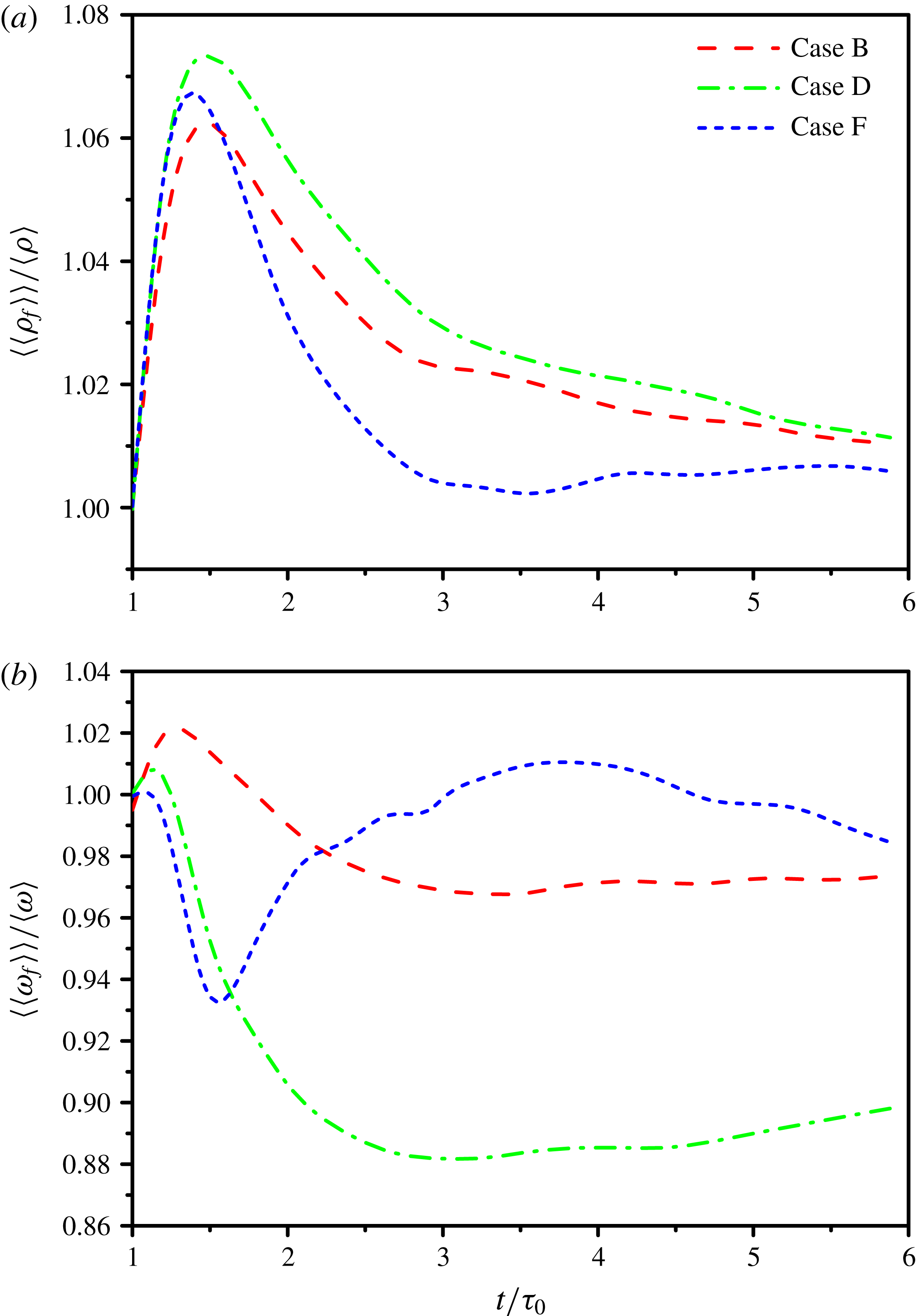
Time development of the normalized averaged (a) fluid density and (b) vorticity magnitude at the particle positions.

Figure 20 shows the temporal evolution of the normalized Lagrangian ensemble-averaged
 $(\langle \langle \rangle \rangle )$
fluid density
 $\langle \langle \unicode[STIX]{x1D70C}_{f}\rangle \rangle /\langle \unicode[STIX]{x1D70C}\rangle$
and vorticity magnitude
 $\langle \langle \unicode[STIX]{x1D714}_{f}\rangle \rangle /\langle \unicode[STIX]{x1D714}\rangle$
at the particle positions. The figures further demonstrate that particles tend to accumulate in the regions with high density and low vorticity, and such a tendency becomes more significant when the Stokes number of particles is close to 1. As the inertia of microparticles (Case B) and critical particles (Case D) is relatively small, these particles tend to follow the streamlines of fluid and stay in the vortex cores with high vorticity at the initial time when particles are injected, resulting in the increment of the normalized averaged vorticity at the particle positions. However, the vorticity will decay with the temporal evolution and particles keep their momentum longer than fluid. Some particles with relatively larger velocity will be ejected out of the vortex cores and accumulate in low-vorticity regions, instead of entering new vortex cores. Thus, the normalized averaged vorticity at the particle positions gradually decreases after the initial injection time. Conversely, large particles (Case F) have larger inertia and will be ejected out of the vortex cores with high vorticity at the initial injection time, resulting in the decrement of the normalized averaged vorticity at the particle positions. Then, since the decay rate of the particle velocities is far smaller than that of fluid velocities, the motion of large particles is hardly influenced by the surrounding fluid and can cross the trajectories of fluid points. Therefore, the distribution of large particles tend to be uniform and the normalized averaged vorticity at the particle positions increases. The fluctuations of the normalized vorticity magnitude seen by particles at the initial injection time result from the effects of particle initial conditions, which will be avoided in the following discussions.
4.4.2 Mechanisms for the modification of turbulent kinetic energy
In order to explain the physical mechanism by which the particles modify TKE, we analyse the transport equations of turbulent kinetic energy obtained from the continuity equation (2.1) and the momentum equation (2.2), which is shown as
 $$\begin{eqnarray}\frac{\unicode[STIX]{x2202}E_{k}(t)}{\unicode[STIX]{x2202}t}=\unicode[STIX]{x1D6F9}_{d}(t)-\unicode[STIX]{x1D700}(t)+\unicode[STIX]{x1D6F9}_{p}(t),\end{eqnarray}$$
where
 $\unicode[STIX]{x1D6F9}_{d}(t)=\langle p\unicode[STIX]{x1D703}/rM^{2}\rangle$
is the pressure-dilatation transfer rate and
 $\unicode[STIX]{x1D700}(t)$
is the viscous dissipation rate. Here
 $\unicode[STIX]{x1D6F9}_{p}(t)$
is the two-way interaction energy rate
 $$\begin{eqnarray}\unicode[STIX]{x1D6F9}_{p}(t)=-\unicode[STIX]{x1D6F7}_{m}\left\langle \left\langle \frac{f_{1}}{\unicode[STIX]{x1D70F}_{p}}(u_{p,i}u_{p,i}-u_{p,i}v_{p,i})\right\rangle \right\rangle ,\end{eqnarray}$$
where
 $\unicode[STIX]{x1D6F7}_{m}=\unicode[STIX]{x1D70C}\unicode[STIX]{x1D719}_{m}=\unicode[STIX]{x1D70C}_{p}N_{p}V_{p}/V_{f}$
.
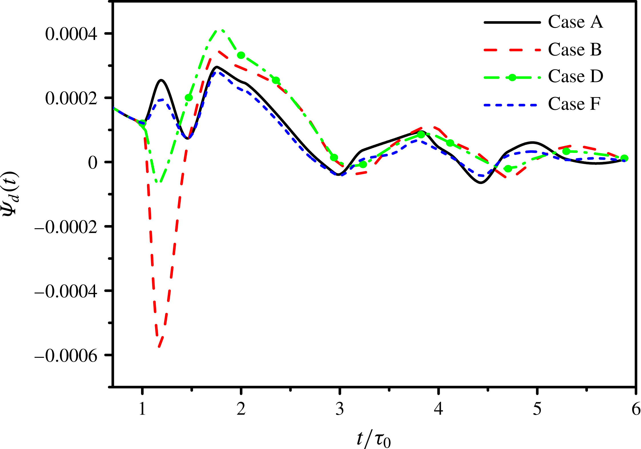
Time development of the pressure-dilatation transfer rate.

First, we consider the pressure-dilatation transfer rate, which is shown in figure 21. This rate does not influence the change of the total energy
 $E$
, but affects the energy transfer between the turbulent kinetic energy
 $E_{k}$
and the internal energy
 $E_{i}$
. The local pressure-dilatation transfer rate
 $P\unicode[STIX]{x1D703}/rM^{2}$
is positive in the expansion regions and negative in the compression regions, but the whole contribution of
 $\langle P\unicode[STIX]{x1D703}/rM^{2}\rangle$
to the turbulent kinetic energy is relatively small (Wang et al.
Reference Wang, Shi, Wang, Xiao, He and Chen2012a
). The figure shows that microparticles (Case B) and critical particles (Case D) enhance the oscillations of
 $\unicode[STIX]{x1D6F9}_{d}(t)$
, while large particles (Case F) suppress the oscillations of
 $\unicode[STIX]{x1D6F9}_{d}(t)$
, resulting in the different temporal fluctuations of TKE in figure 4(b). With the increase of
 $St_{0}$
, the oscillation amplitude of
 $\unicode[STIX]{x1D6F9}_{d}(t)$
reduces, which is also responsible for the attenuation of the temporal fluctuations of TKE.
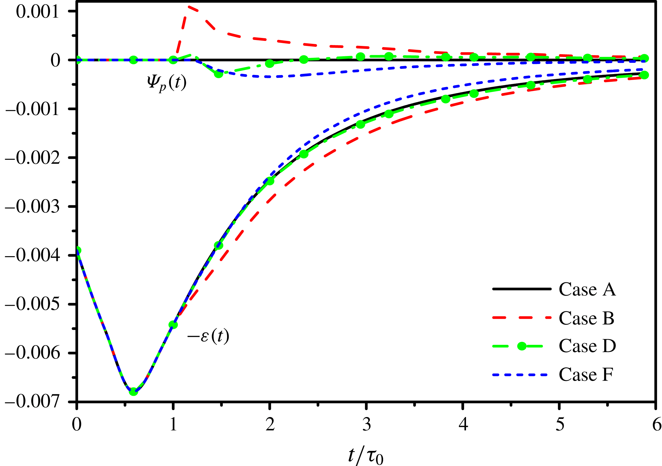
Time development of the two-way interaction energy rate
 $\unicode[STIX]{x1D6F9}_{p}(t)$
and the opposite of the viscous dissipation rate
 $-\unicode[STIX]{x1D700}(t)$
.

Next, we consider the modifications of the viscous dissipation rate
 $\unicode[STIX]{x1D700}(t)$
shown in figure 22. Compared with the particle-free flow (Case A), microparticles (Case B) enhance the viscous dissipation rate; critical particles (Case D) have weak effect on the viscous dissipation rate; large particles (Case F) reduce the viscous dissipation rate. The modifications of
 $\unicode[STIX]{x1D700}(t)$
are similar to that of TKE in figure 4, and also demonstrated in the modifications of the characteristic length scales in figure 7.
In compressible flows, the viscous dissipation rate can be decomposed into three components, which is expressed as
 $$\begin{eqnarray}\unicode[STIX]{x1D700}=\frac{1}{Re}\langle \unicode[STIX]{x1D707}\unicode[STIX]{x1D714}^{2}\rangle +\frac{4}{3Re}\langle \unicode[STIX]{x1D707}\unicode[STIX]{x1D703}^{2}\rangle +\frac{2}{Re}\left\langle \unicode[STIX]{x1D707}\left(\frac{\unicode[STIX]{x2202}u_{i}}{\unicode[STIX]{x2202}x_{j}}\frac{\unicode[STIX]{x2202}u_{j}}{\unicode[STIX]{x2202}x_{i}}-\unicode[STIX]{x1D703}^{2}\right)\right\rangle ,\end{eqnarray}$$
where
 $\unicode[STIX]{x1D700}_{s}=\langle \unicode[STIX]{x1D707}\unicode[STIX]{x1D714}^{2}\rangle /Re$
is the solenoidal dissipation rate,
 $\unicode[STIX]{x1D700}_{c}=4\langle \unicode[STIX]{x1D707}\unicode[STIX]{x1D703}^{2}\rangle /(3Re)$
is the dilatational dissipation rate and
 $\unicode[STIX]{x1D700}_{m}=(2/Re)\langle \unicode[STIX]{x1D707}((\unicode[STIX]{x2202}u_{i}/\unicode[STIX]{x2202}x_{j})(\unicode[STIX]{x2202}u_{j}/\unicode[STIX]{x2202}x_{i})-\unicode[STIX]{x1D703}^{2})\rangle$
is the mixed term. Compared with the incompressible turbulence, the dissipation rate of the compressible turbulence includes the extra influence of the dilatation. In addition, the influence of the dilatational dissipation rate is significant especially in the high compression regions (or shocklet regions). The mixed term is relatively very small and can be neglected. In our simulations, the solenoidal dissipation rate and the dilatational dissipation rate contribute more than 96 % of the total viscous dissipation rate. Thus, only
 $\unicode[STIX]{x1D700}_{s}$
and
 $\unicode[STIX]{x1D700}_{c}$
are considered in this paper.
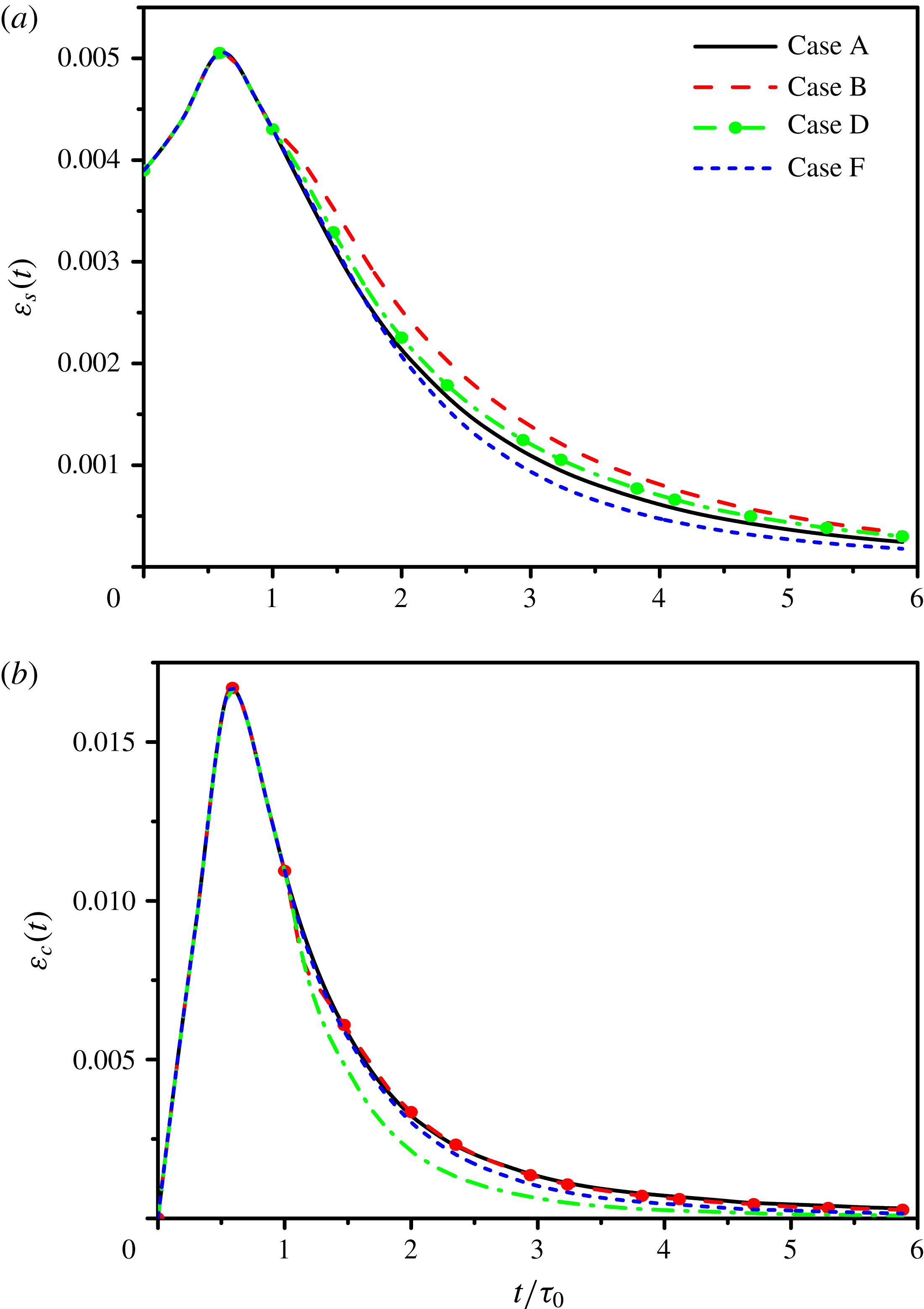
Time development of (a) the solenoidal dissipation rate and (b) the dilatational dissipation rate.

Figure 23 shows the temporal evolution of the solenoidal dissipation rate and the dilatational dissipation rate. The solenoidal dissipation rate is associated with the rotational motion of fluid, and the modifications of
 $\unicode[STIX]{x1D700}_{s}$
are the same as that of the r.m.s. of the vorticity in figure 6. The dilatational dissipation rate is related to the compressibility of the turbulence field, and the modifications of
 $\unicode[STIX]{x1D700}_{c}$
are identical to that of the r.m.s. of the dilatation in figure 10. Microparticles (Case B) augment the solenoidal dissipation rate, but weakly attenuate the dilatational dissipation rate. Thus, the net result of these two dissipation rates is the enhancement of the total viscous dissipation rate compared with Case A according to (4.10). Critical particles (Case D) augment the solenoidal dissipation rate, but attenuate the dilatational dissipation rate. The magnitude of the enhancement of
 $\unicode[STIX]{x1D700}_{s}$
is close to the magnitude of the reduction of
 $\unicode[STIX]{x1D700}_{c}$
, which results in the total viscous dissipation rate nearly identical to that of Case A. Large particles (Case F) attenuate both the solenoidal dissipation rate and the dilatational dissipation rate, and the total viscous dissipation rate is hence reduced.
Finally, we analyse the physical mechanisms of the modifications of the two-way interaction energy rate
 $\unicode[STIX]{x1D6F9}_{p}(t)$
, as shown in figure 22. The magnitude of
 $\unicode[STIX]{x1D6F9}_{p}(t)$
is larger than the magnitude of the modifications of
 $\unicode[STIX]{x1D700}$
, and the two-way interaction energy rate is therefore the main factor to determine the modulation to TKE by particles based on the analysis of Balachandar & Eaton (Reference Balachandar and Eaton2010). With the temporal evolution, the Stokes number of particles decreases and the vector alignment between particles and fluid increases, resulting in the decrement of the magnitude of
 $\unicode[STIX]{x1D6F9}_{p}(t)$
after the initial period. The drag force of microparticles (Case B) provides the positive work on
 $\text{d}E_{k}(t)/\text{d}t$
in (4.8), and reduces the decay rate of TKE compared with the particle-free flow. The drag force of large particles (Case F) provides the negative work on
 $\text{d}E_{k}(t)/\text{d}t$
, resulting in the enhancement of the decay rate of TKE at early times. However,
 $\unicode[STIX]{x1D6F9}_{p}(t)$
of critical particles (Case D) becomes negative at early times (
 $t<2.35\unicode[STIX]{x1D70F}_{0}$
) and positive later (
 $t\geqslant 2.35\unicode[STIX]{x1D70F}_{0}$
), which is relatively small and slightly enhances the decay rate of TKE at early times. The modifications of
 $\unicode[STIX]{x1D6F9}_{p}(t)$
are similar to that in incompressible turbulence (Ferrante & Elghobashi Reference Ferrante and Elghobashi2003), which is perhaps due to the same drag force and governing equations for particle motion (2.8)–(2.10).
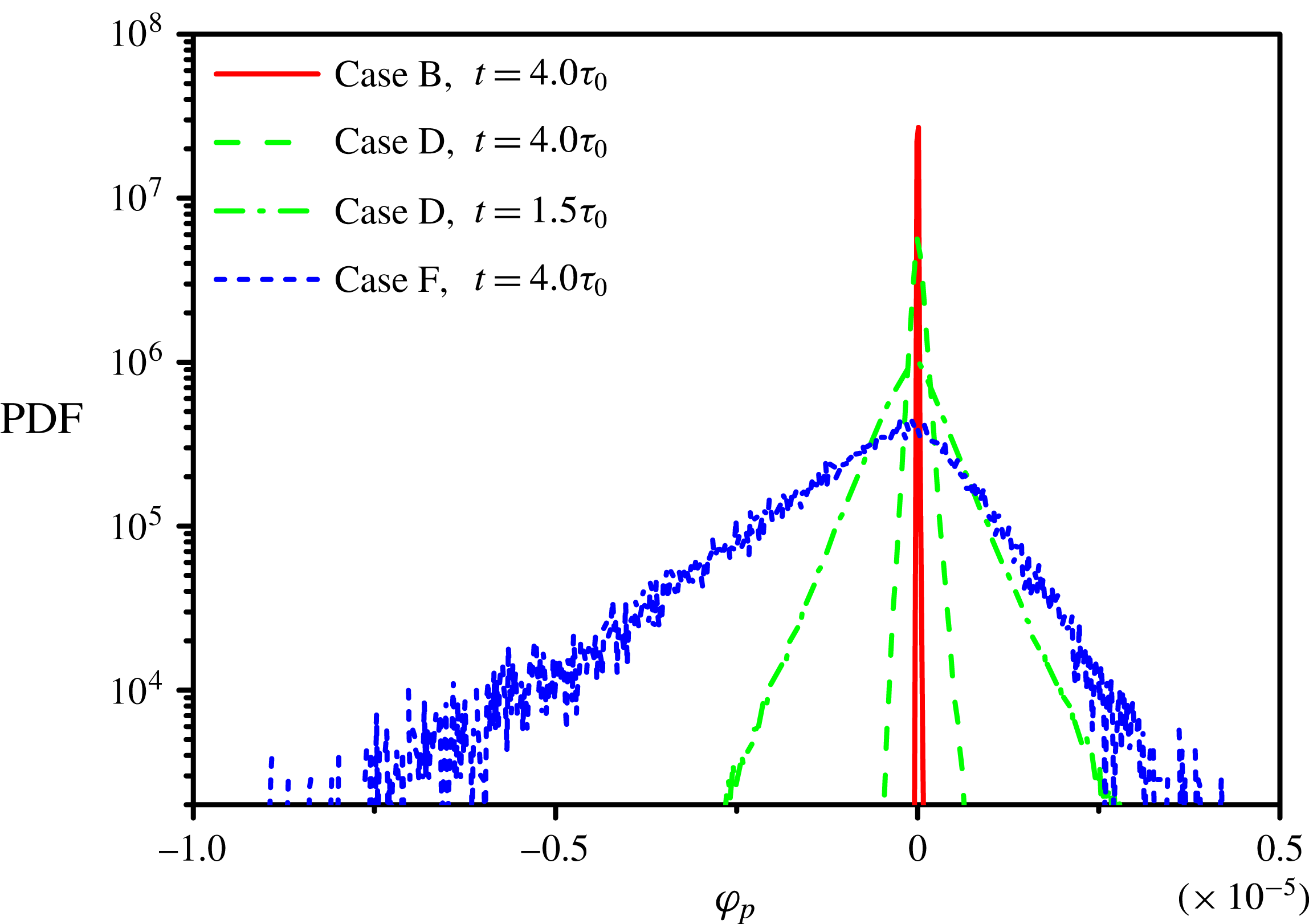
Probability density functions of the two-way interaction energy rate of a single particle.

Figure 24 shows the PDFs of the two-way interaction energy rate of a single particle, which is given by
 $$\begin{eqnarray}\unicode[STIX]{x1D711}_{p}=-m_{p}\frac{f_{1}}{\unicode[STIX]{x1D70F}_{p}}(u_{p,i}u_{p,i}-u_{p,i}v_{p,i}).\end{eqnarray}$$
With the increment of the particle diameter, the two-way interaction energy rate of a single particle also increases. For microparticles (Case B), the PDFs are skewed to the positive value, resulting in the whole two-way interaction energy rate being positive. For large particles (Case F), the left tail of the PDFs is longer than the right tail, and
 $\unicode[STIX]{x1D6F9}_{p}(t)$
is hence negative. For critical particles (Case D), the PDFs shift in the negative direction at
 $t=1.5\unicode[STIX]{x1D70F}_{0}$
but become skewed to the positive side at
 $t=4\unicode[STIX]{x1D70F}_{0}$
, so
 $\unicode[STIX]{x1D6F9}_{p}(t)$
is negative at early times (
 $t<2.35\unicode[STIX]{x1D70F}_{0}$
) and positive later (
 $t\geqslant 2.35\unicode[STIX]{x1D70F}_{0}$
).
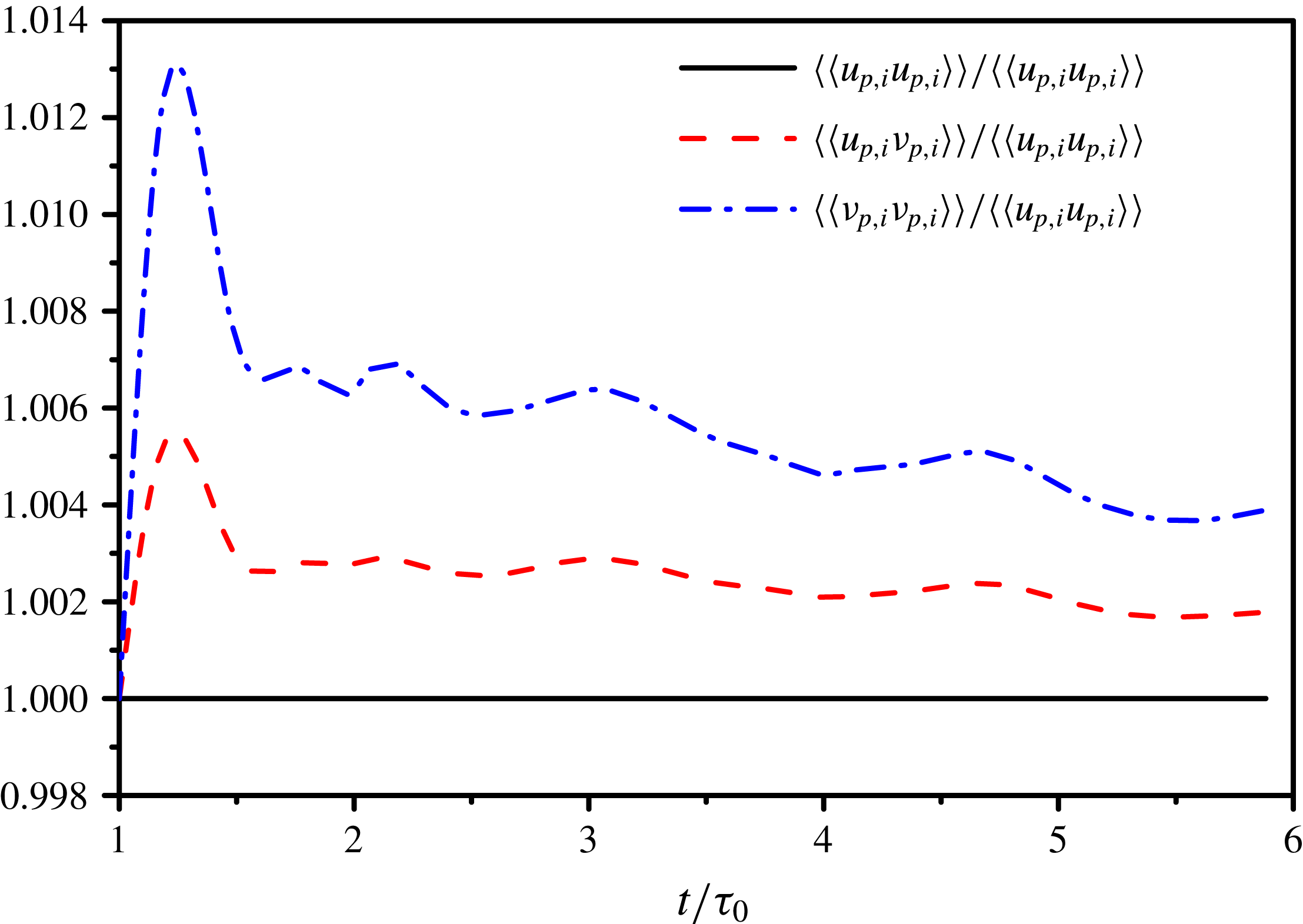
Time development of the fluid velocity autocorrelation
 $\langle \langle u_{p,i}u_{p,i}\rangle \rangle$
, the correlation
 $\langle \langle u_{p,i}v_{p,i}\rangle \rangle$
between fluid velocity and particle velocity and the particle velocity autocorrelation
 $\langle \langle v_{p,i}v_{p,i}\rangle \rangle$
, all normalized by
 $\langle \langle u_{p,i}u_{p,i}\rangle \rangle$
, for Case B.

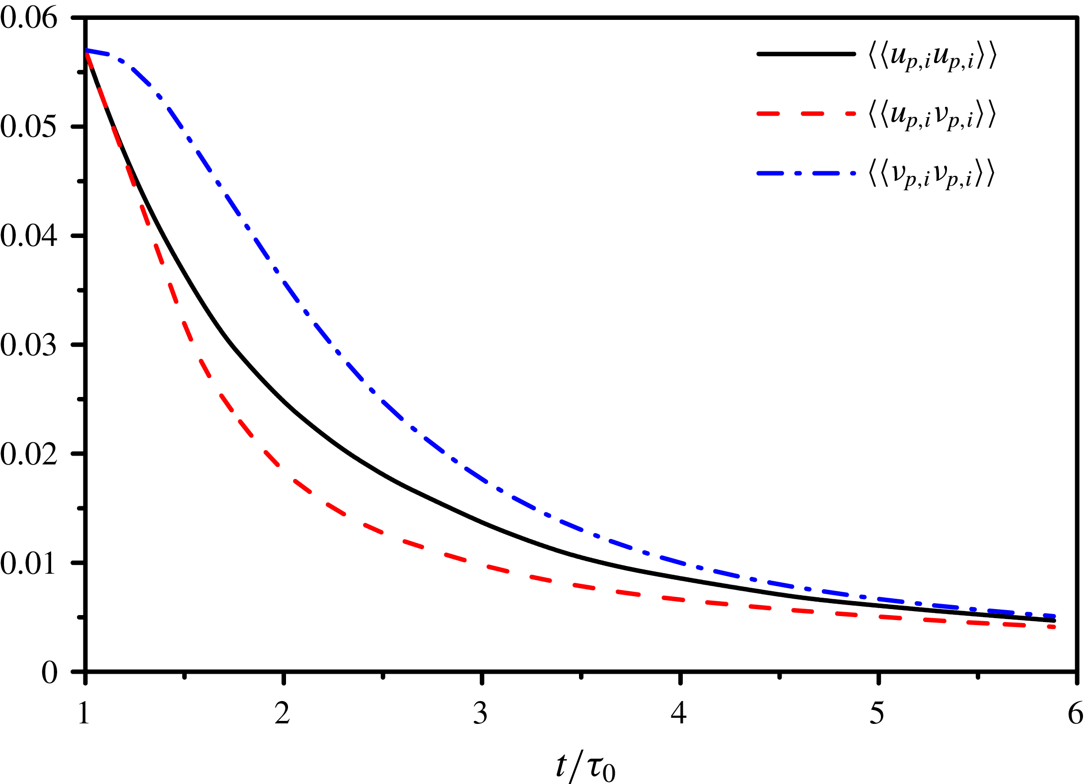
Time development of the fluid velocity autocorrelation
 $\langle \langle u_{p,i}u_{p,i}\rangle \rangle$
, the correlation
 $\langle \langle u_{p,i}v_{p,i}\rangle \rangle$
between fluid velocity and particle velocity and the particle velocity autocorrelation
 $\langle \langle v_{p,i}v_{p,i}\rangle \rangle$
for Case F.

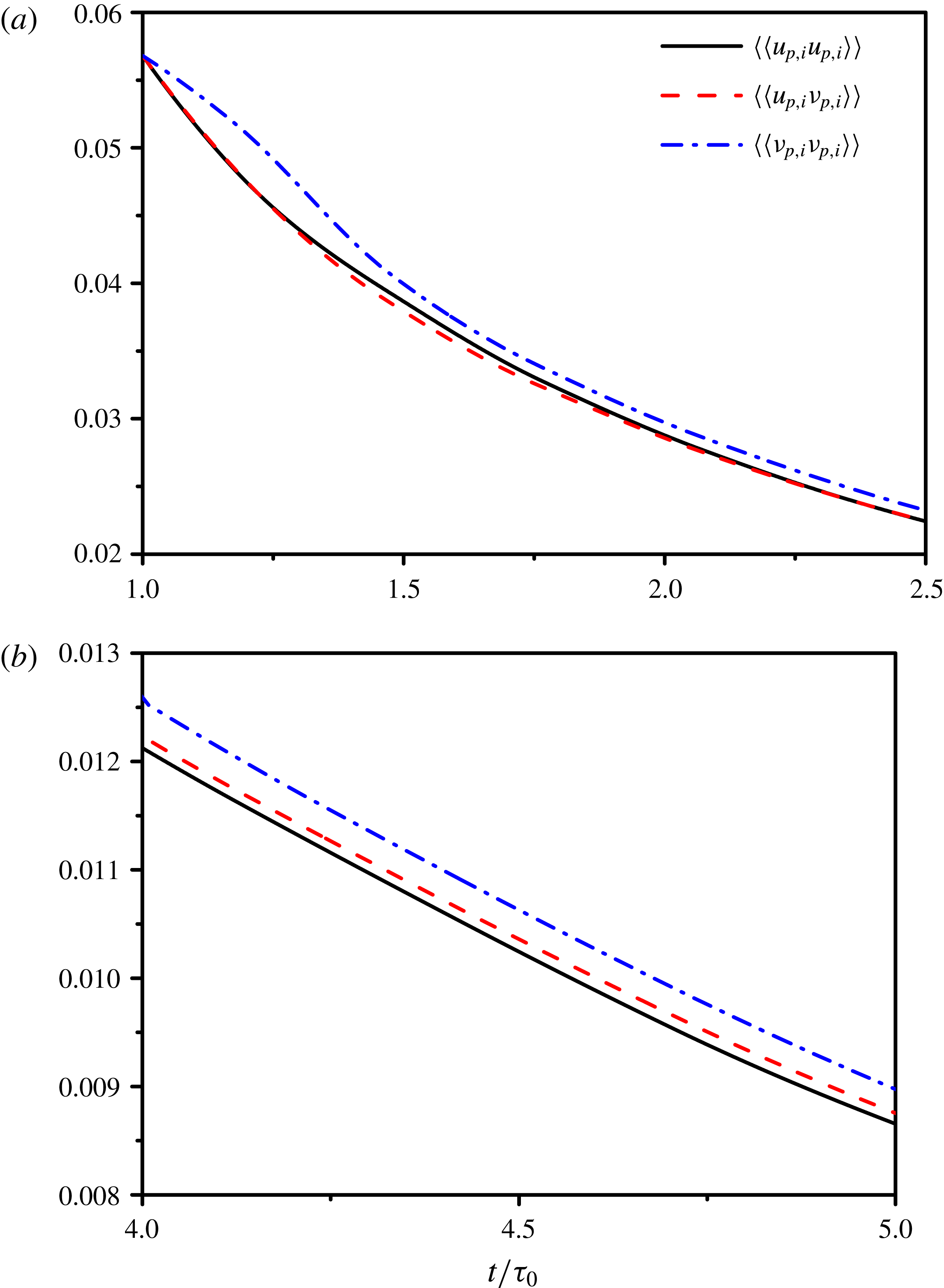
Time development of the fluid velocity autocorrelation
 $\langle \langle u_{p,i}u_{p,i}\rangle \rangle$
, the correlation
 $\langle \langle u_{p,i}v_{p,i}\rangle \rangle$
between fluid velocity and particle velocity and the particle velocity autocorrelation
 $\langle \langle v_{p,i}v_{p,i}\rangle \rangle$
for Case D during time: (a)
 $\unicode[STIX]{x1D70F}_{0}\leqslant t\leqslant 2.5\unicode[STIX]{x1D70F}_{0}$
;(b)
 $4\unicode[STIX]{x1D70F}_{0}\leqslant t\leqslant 5\unicode[STIX]{x1D70F}_{0}$
.

As given in (4.9), the sign of
 $\unicode[STIX]{x1D6F9}_{p}(t)$
is determined by the relative magnitude of the fluid velocity autocorrelation
 $\langle \langle u_{p,i}u_{p,i}\rangle \rangle$
and the correlation
 $\langle \langle u_{p,i}v_{p,i}\rangle \rangle$
between fluid velocity and particle velocity. Figures 25–27 show the temporal evolution of the fluid velocity autocorrelation
 $\langle \langle u_{p,i}u_{p,i}\rangle \rangle$
, the correlation
 $\langle \langle u_{p,i}v_{p,i}\rangle \rangle$
between fluid velocity and particle velocity and the particle velocity autocorrelation
 $\langle \langle v_{p,i}v_{p,i}\rangle \rangle$
, which are the Lagrangian one-point one-time correlations (Libby Reference Libby1996).
 $\langle \langle u_{p,i}u_{p,i}\rangle \rangle$
is the Lagrangian ensemble average of the square of the fluid velocity at the particle position,
 $\langle \langle u_{p,i}v_{p,i}\rangle \rangle$
is the Lagrangian ensemble average of the scalar product of the fluid velocity and the particle velocity at the particle position and
 $\langle \langle v_{p,i}v_{p,i}\rangle \rangle$
is the Lagrangian ensemble average of the square of the particle velocity.
Due to the higher inertia of microparticles compared with the carrier fluid, the decay rate of particle velocities is smaller than that of the surrounding fluid velocities. Therefore, the particle velocity autocorrelation
 $\langle \langle v_{p,i}v_{p,i}\rangle \rangle$
is larger than the surrounding fluid velocity autocorrelation
 $\langle \langle u_{p,i}u_{p,i}\rangle \rangle$
as shown in figure 25. Because microparticles mostly follow the fluid points’ trajectories, the correlation
 $\langle \langle u_{p,i}v_{p,i}\rangle \rangle$
between fluid velocity and particle velocity keeps larger than
 $\langle \langle u_{p,i}u_{p,i}\rangle \rangle$
, resulting in the two-way interaction energy rate
 $\unicode[STIX]{x1D6F9}_{p}(t)$
being positive.
Large particles, as microparticles, also keep their momentum longer than the surrounding fluid due to the high inertia, and the particle velocity autocorrelation
 $\langle \langle v_{p,i}v_{p,i}\rangle \rangle$
is larger than the surrounding fluid velocity autocorrelation
 $\langle \langle u_{p,i}u_{p,i}\rangle \rangle$
, as shown in figure 26. However, the correlation
 $\langle \langle u_{p,i}v_{p,i}\rangle \rangle$
between fluid velocity and particle velocity is smaller than the surrounding fluid velocity autocorrelation
 $\langle \langle u_{p,i}u_{p,i}\rangle \rangle$
, as large particles move randomly and can cross the trajectories of the fluid points. Consequently, large particles are obstacles to fluid motion and the two-way interaction energy rate
 $\unicode[STIX]{x1D6F9}_{p}(t)$
becomes negative.
At early times (
 $t<2.35\unicode[STIX]{x1D70F}_{0}$
), critical particles move out of the initial vortical structures of surrounding fluid and cross the fluid points’ trajectories, as large particles do. Therefore,
 $\langle \langle u_{p,i}v_{p,i}\rangle \rangle$
is smaller than
 $\langle \langle u_{p,i}u_{p,i}\rangle \rangle$
, as shown in figure 27(a), and the two-way interaction energy rate
 $\unicode[STIX]{x1D6F9}_{p}(t)$
is negative at the early times. At later times (
 $t\geqslant 2.35\unicode[STIX]{x1D70F}_{0}$
) after critical particles have escaped from the vortex cores, they do not have enough inertia to enter new vortex cores, but rather accumulate in the peripheries of the vortex cores. Because of the high inertia, particles keep their kinetic energy longer than the surrounding fluid and the particle velocity autocorrelation
 $\langle \langle v_{p,i}v_{p,i}\rangle \rangle$
is larger than the surrounding fluid velocity autocorrelation
 $\langle \langle u_{p,i}u_{p,i}\rangle \rangle$
. Once the particles accumulate in the peripheries of the vortex cores, they tend to follow the surrounding fluid points’ trajectories like microparticles. Thus, the correlation
 $\langle \langle u_{p,i}v_{p,i}\rangle \rangle$
between fluid velocity and particle velocity is larger than the surrounding fluid velocity autocorrelation
 $\langle \langle u_{p,i}u_{p,i}\rangle \rangle$
in figure 27(b), and the two-way interaction energy rate
 $\unicode[STIX]{x1D6F9}_{p}(t)$
is positive at the later times.
4.4.3 Mechanisms for the modification of the rotational motion of fluid
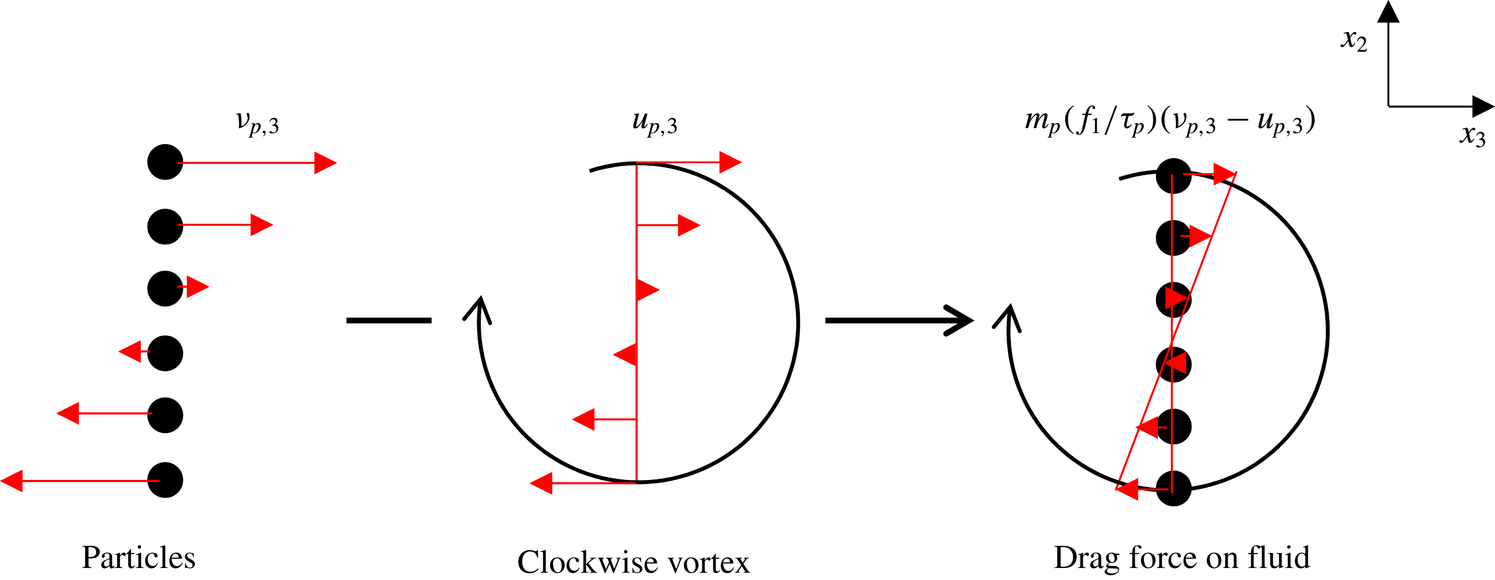
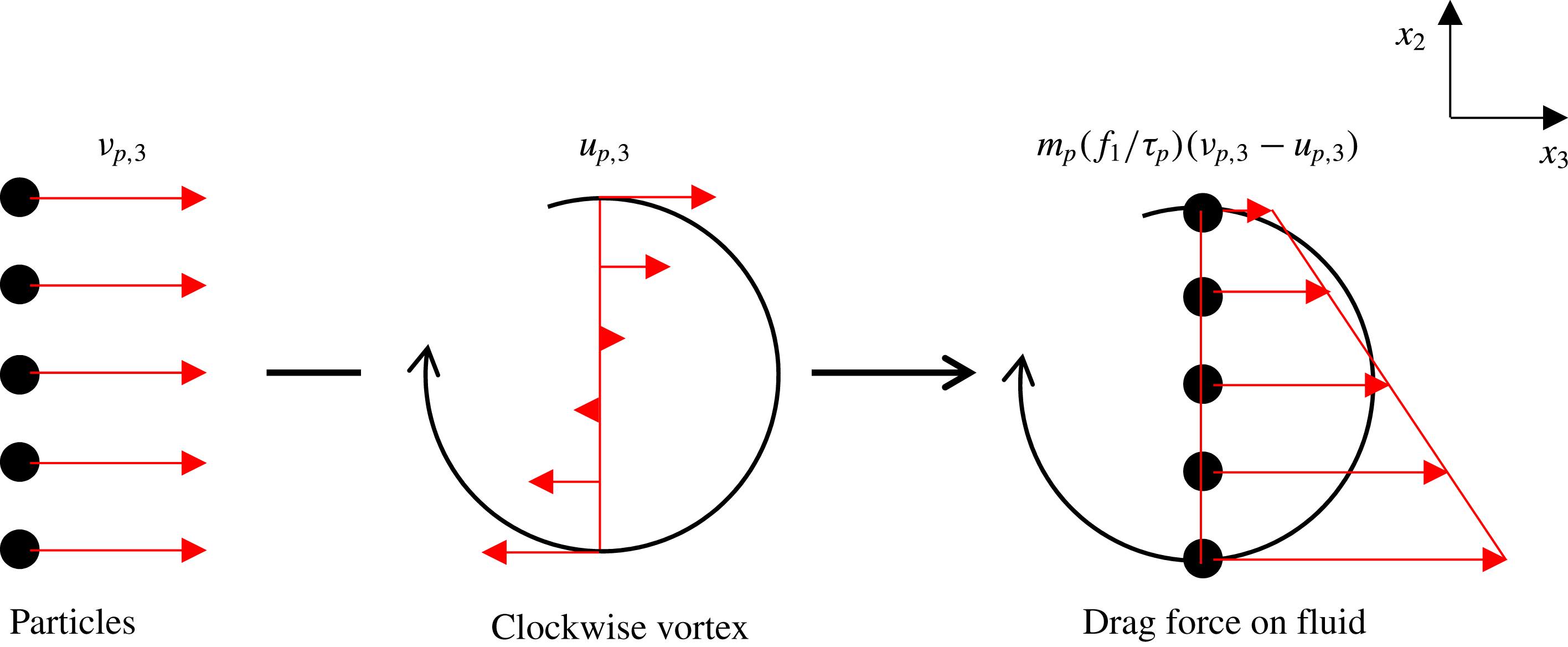
The rotational motion of fluid is associated with the vorticity, so we analyse the temporal evolution of the vorticity in different cases to reveal the underlying physical mechanisms for the modification of the rotational motion of fluid. In this subsection, particles are treated as a kind of hypothetical fluids, and the velocity derivatives and the vorticity of Lagrangian particles can be considered. The vorticity of particles is positive if particles rotate in the clockwise direction; the vorticity of particles is negative if particles rotate in the anticlockwise direction.
The transport equation of vorticity in compressible turbulence can be obtained by taking the curl of the momentum equation (2.2)
 $$\begin{eqnarray}\frac{\text{D}\unicode[STIX]{x1D714}}{\text{D}t}=-\unicode[STIX]{x1D714}\unicode[STIX]{x1D735}\boldsymbol{\cdot }V-\frac{\unicode[STIX]{x1D735}P\times \unicode[STIX]{x1D735}\unicode[STIX]{x1D70C}}{\unicode[STIX]{x1D6FE}M^{2}\unicode[STIX]{x1D70C}^{2}}+\frac{1}{Re}\unicode[STIX]{x1D708}\unicode[STIX]{x1D6FB}^{2}\unicode[STIX]{x1D714}+\unicode[STIX]{x1D735}\times \left(\frac{1}{\unicode[STIX]{x1D70C}}\unicode[STIX]{x1D711}_{u}\right),\end{eqnarray}$$
where the bulk viscosity is negligible and the shear viscosity is supposed to be constant. Taking the component in
 $x_{1}$
direction of the vorticity vector, we can obtain the transport equation for
 $\unicode[STIX]{x1D714}_{1}$
 $$\begin{eqnarray}\displaystyle \frac{\text{d}\unicode[STIX]{x1D714}_{1}}{\text{d}t} & = & \displaystyle \unicode[STIX]{x1D714}_{j}\frac{\unicode[STIX]{x2202}u_{1}}{\unicode[STIX]{x2202}x_{j}}-\frac{1}{\unicode[STIX]{x1D6FE}M^{2}\unicode[STIX]{x1D70C}^{2}}\left[\frac{\unicode[STIX]{x2202}p}{\unicode[STIX]{x2202}x_{3}}\frac{\unicode[STIX]{x2202}\unicode[STIX]{x1D70C}}{\unicode[STIX]{x2202}x_{2}}-\frac{\unicode[STIX]{x2202}p}{\unicode[STIX]{x2202}x_{2}}\frac{\unicode[STIX]{x2202}\unicode[STIX]{x1D70C}}{\unicode[STIX]{x2202}x_{3}}\right]\nonumber\\ \displaystyle & & \displaystyle +\,\frac{1}{Re}\left\{\frac{\unicode[STIX]{x2202}}{\unicode[STIX]{x2202}x_{2}}\left(\frac{1}{\unicode[STIX]{x1D70C}}\frac{\unicode[STIX]{x2202}\unicode[STIX]{x1D70E}_{3j}}{\unicode[STIX]{x2202}x_{j}}\right)-\frac{\unicode[STIX]{x2202}}{\unicode[STIX]{x2202}x_{3}}\left(\frac{1}{\unicode[STIX]{x1D70C}}\frac{\unicode[STIX]{x2202}\unicode[STIX]{x1D70E}_{2j}}{\unicode[STIX]{x2202}x_{j}}\right)\right\}+\frac{\unicode[STIX]{x2202}}{\unicode[STIX]{x2202}x_{2}}\left(\frac{\unicode[STIX]{x1D711}_{u3}}{\unicode[STIX]{x1D70C}}\right)-\frac{\unicode[STIX]{x2202}}{\unicode[STIX]{x2202}x_{3}}\left(\frac{\unicode[STIX]{x1D711}_{u2}}{\unicode[STIX]{x1D70C}}\right)\!.\quad\end{eqnarray}$$
Since microparticles (Case B) respond fast to the fluid motion, most particles remain in the initial vortex cores of the surrounding fluid shown in figure 17(b), and rotate as the fluid points’ trajectories. Figure 28 shows a schematic of the interaction between microparticles and the surrounding fluid when particles remain in a simplified two-dimensional clockwise vortex in the
 $x_{2}x_{3}$
plane. Due to the high inertia of particles, microparticles keep their momentum longer than the surrounding fluid and the vorticity of particles is larger than that of the fluid. Therefore, microparticles exert a force with positive effect on the surrounding fluid, and augment the rotational motion of fluid compared with the particle-free flow (Case A). The enhancement of the fluid vorticity also causes the reduction of the characteristic length scales in figure 7.
Critical particles (Case D) move out of the vortical structures with high vorticity soon after injection and mostly accumulate in the peripheries of the vortex cores with low vorticity, so particles seldom remain in the high-vorticity regions. The two-way coupling force
 $\unicode[STIX]{x1D711}_{u}\approx 0$
inside these vortex cores and the source term in the transport equation (4.12)
 $\unicode[STIX]{x1D735}\times \unicode[STIX]{x1D711}_{u}$
is very small. Therefore, the r.m.s. of vorticity is closest to that of Case A compared with the other cases in figure 6. On the other hand, due to the high compressibility of the turbulence field, some critical particles also tend to collect in the downstream regions of the shocklets with high vorticity. Consequently, these particles, as microparticles, exert a positive work on the vorticity of the surrounding fluid, and the rotational motion of fluid is slightly augmented. Since the vortical structures are hardly modified, the characteristic length scales are nearly identical to those of Case A in figure 7.
Schematic of the drag interaction between microparticles and a simplified two-dimensional clockwise vortex
 $(\unicode[STIX]{x1D714}_{1}>0)$
.

Schematic of the drag interaction between large particles and a simplified two-dimensional clockwise vortex
 $(\unicode[STIX]{x1D714}_{1}>0)$
.

Large particles (Case F) move randomly with nearly uniform velocity and cross the vortex cores of the surrounding fluid, which is different from the microparticles, and the influence on the vorticity is also different. Figure 29 shows a schematic of the interaction between large particles and the surrounding fluid when particles moving in the
 $x_{3}$
direction encounter a simplified two-dimensional clockwise vortex in the
 $x_{2}x_{3}$
plane. Large particles exert a reverse drag force
 $m_{p}f_{1}/\unicode[STIX]{x1D70F}_{p}(v_{p,3}-u_{p,3})$
on the fluid in the
 $x_{3}$
direction, which is proportional to the relative velocity
 $(v_{p,3}-u_{p,3})$
. As the gradient of the drag force is negative in the
 $x_{2}$
direction, the interaction produces a counterclockwise torque on the vortex, which results in the reduction of the vorticity. Therefore, the rotational motion of fluid is also attenuated.
For further analysis, the source term in the transport equation for
 $\unicode[STIX]{x1D714}_{1}$
(4.13) is investigated, which is the curl of the drag force exerted on the fluid
 $$\begin{eqnarray}\displaystyle & & \displaystyle \frac{\unicode[STIX]{x2202}}{\unicode[STIX]{x2202}x_{2}}\left(\frac{\unicode[STIX]{x1D711}_{u3}}{\unicode[STIX]{x1D70C}}\right)-\frac{\unicode[STIX]{x2202}}{\unicode[STIX]{x2202}x_{3}}\left(\frac{\unicode[STIX]{x1D711}_{u2}}{\unicode[STIX]{x1D70C}}\right)\nonumber\\ \displaystyle & & \displaystyle \quad \approx \,\frac{1}{\unicode[STIX]{x0394}V\cdot Re}\mathop{\sum }_{n_{p}}3\unicode[STIX]{x03C0}\unicode[STIX]{x1D708}d_{p}f_{1}\left[\left(\frac{\unicode[STIX]{x2202}v_{p,3}}{\unicode[STIX]{x2202}x_{p,2}}-\frac{\unicode[STIX]{x2202}v_{p,2}}{\unicode[STIX]{x2202}x_{p,3}}\right)-\left(\frac{\unicode[STIX]{x2202}u_{p,3}}{\unicode[STIX]{x2202}x_{p,2}}-\frac{\unicode[STIX]{x2202}u_{p,2}}{\unicode[STIX]{x2202}x_{p,3}}\right)\right].\end{eqnarray}$$
Since large particles move randomly in the field, their motion can be treated as a kind of hypothetical irrotational flow, which means the vorticity of particles is approximate to 0 and
 $\unicode[STIX]{x2202}v_{p,3}/\unicode[STIX]{x2202}x_{p,2}-\unicode[STIX]{x2202}v_{p,2}/\unicode[STIX]{x2202}x_{p,3}\approx 0$
. In addition,
 $\unicode[STIX]{x1D714}_{1}$
is positive in the clockwise vortex and
 $\unicode[STIX]{x2202}u_{p,3}/\unicode[STIX]{x2202}x_{p,2}-\unicode[STIX]{x2202}u_{p,2}/\unicode[STIX]{x2202}x_{p,3}>0$
. Therefore, we can infer that the source term
 $\unicode[STIX]{x2202}(\unicode[STIX]{x1D711}_{u3}/\unicode[STIX]{x1D70C})/\unicode[STIX]{x2202}x_{2}-\unicode[STIX]{x2202}(\unicode[STIX]{x1D711}_{u2}/\unicode[STIX]{x1D70C})/\unicode[STIX]{x2202}x_{3}$
in (4.14) is negative in the clockwise vortices (or positive in the anticlockwise vortices), resulting in the enhancement of the decay rate of
 $|\unicode[STIX]{x1D714}_{1}|$
. Accordingly, large particles attenuate the vorticity and reduce the lifetime of vortices, which also causes the enhancement of the characteristic length scales in figure 7.
4.4.4 Mechanisms for the modification of the compressibility of the turbulence field
The compressibility of the turbulence field is related to the dilatation, so the temporal evolution of the dilatation in different cases is investigated to reveal the underlying physical mechanisms for the modification of the compressibility of the turbulence field. In this subsection, particles are also treated as a kind of hypothetical fluids, and the velocity divergence of Lagrangian particles can be considered, which represents the particle compressibility (Maxey Reference Maxey1987; Goto & Vassilicos Reference Goto and Vassilicos2008). The difference between the particle dilatation and the fluid dilatation at the particle positions
 $\unicode[STIX]{x1D735}\boldsymbol{\cdot }\boldsymbol{v}_{p}-\unicode[STIX]{x1D735}\boldsymbol{\cdot }\boldsymbol{u}_{p}$
is positive if particles spread out;
 $\unicode[STIX]{x1D735}\boldsymbol{\cdot }\boldsymbol{v}_{p}-\unicode[STIX]{x1D735}\boldsymbol{\cdot }\boldsymbol{u}_{p}$
is negative if particles accumulate. Therefore, particles have the tendency to collect in the regions where
 $\unicode[STIX]{x1D735}\boldsymbol{\cdot }\boldsymbol{v}_{p}-\unicode[STIX]{x1D735}\boldsymbol{\cdot }\boldsymbol{u}_{p}$
is negative (see appendix B for the verification).
The transport equation of the dilatation in compressible turbulence can be obtained by taking the divergence of the momentum equation (2.2)
 $$\begin{eqnarray}\frac{\text{d}\unicode[STIX]{x1D703}}{\text{d}t}=-\frac{\unicode[STIX]{x2202}u_{j}}{\unicode[STIX]{x2202}x_{i}}\frac{\unicode[STIX]{x2202}u_{i}}{\unicode[STIX]{x2202}x_{j}}-\frac{1}{\unicode[STIX]{x1D6FE}M^{2}}\frac{\unicode[STIX]{x2202}}{\unicode[STIX]{x2202}x_{i}}\left(\frac{1}{\unicode[STIX]{x1D70C}}\frac{\unicode[STIX]{x2202}p}{\unicode[STIX]{x2202}x_{i}}\right)+\frac{4\unicode[STIX]{x1D708}}{3Re}\frac{\unicode[STIX]{x2202}^{2}\unicode[STIX]{x1D703}}{\unicode[STIX]{x2202}x_{i}^{2}}+\frac{\unicode[STIX]{x2202}}{\unicode[STIX]{x2202}x_{i}}\left(\frac{1}{\unicode[STIX]{x1D70C}}\unicode[STIX]{x1D711}_{ui}\right),\end{eqnarray}$$
where the influence of density fluctuations on the viscous term is neglected to simplify the discussions (Wang et al.
Reference Wang, Shi, Wang, Xiao and He2012b
). In the one-dimension circumstances, the transport equation of the velocity divergence, taking
 $x_{1}$
direction for example, is reduced to
 $$\begin{eqnarray}\frac{\unicode[STIX]{x2202}}{\unicode[STIX]{x2202}t}\left(\frac{\unicode[STIX]{x2202}u_{1}}{\unicode[STIX]{x2202}x_{1}}\right)+u_{1}\frac{\unicode[STIX]{x2202}^{2}u_{1}}{\unicode[STIX]{x2202}x_{1}^{2}}=-\left(\frac{\unicode[STIX]{x2202}u_{1}}{\unicode[STIX]{x2202}x_{1}}\right)^{2}-\frac{1}{\unicode[STIX]{x1D6FE}M^{2}}\frac{\unicode[STIX]{x2202}}{\unicode[STIX]{x2202}x_{1}}\left(\frac{1}{\unicode[STIX]{x1D70C}}\frac{\unicode[STIX]{x2202}p}{\unicode[STIX]{x2202}x_{1}}\right)+\frac{4\unicode[STIX]{x1D708}}{3Re}\frac{\unicode[STIX]{x2202}^{3}u_{1}}{\unicode[STIX]{x2202}x_{1}^{3}}+\frac{\unicode[STIX]{x2202}}{\unicode[STIX]{x2202}x_{1}}\left(\frac{\unicode[STIX]{x1D711}_{u1}}{\unicode[STIX]{x1D70C}}\right).\end{eqnarray}$$
Schematic of the drag interaction between particles and a simplified one-dimensional expansion control volume
 $(\unicode[STIX]{x1D703}>0)$
.

Considering a one-dimensional control volume, fluid enters the volume from the left and exits from the right. Taking the situation of the positive velocity divergence as an example, the fluid expands in the control volume and the velocity
 $u_{p,1,out}$
at the outlet is larger than the velocity
 $u_{p,1,in}$
at the inlet. Figure 30 shows a schematic of the interaction between particles and the surrounding fluid when a group of particles encounter a simplified one-dimensional expansion control volume in the
 $x_{1}$
direction. The effect of this interaction is to exert a reverse drag force
 $m_{p}f_{1}/\unicode[STIX]{x1D70F}_{p}(v_{p,1}-u_{p,1})$
on the fluid in the
 $x_{1}$
direction. In addition, because
 $\unicode[STIX]{x1D735}\boldsymbol{\cdot }\boldsymbol{v}_{p}-\unicode[STIX]{x1D735}\boldsymbol{\cdot }\boldsymbol{u}_{p}$
is negative in the regions where particles accumulate, the dilatation of particles is smaller than that of the surrounding fluid and
 $v_{p,1,out}-v_{p,1,in}<u_{p,1,out}-u_{p,1,in}$
. Therefore, the drag force at the inlet is larger than the drag force at the outlet. This means particles, when interacting with an expansion control volume, exert a compression force on the fluid, which in turn prevents the expansion of fluid and hence reduces the fluid dilatation.
For further analysis, the source term in the transport equation for
 $\unicode[STIX]{x1D703}$
(4.15) is investigated, which is the divergence of the drag force exerted on the fluid
 $$\begin{eqnarray}\unicode[STIX]{x1D735}\boldsymbol{\cdot }\left(\frac{1}{\unicode[STIX]{x1D70C}}\unicode[STIX]{x1D753}_{\boldsymbol{u}}\right)\approx \frac{1}{\unicode[STIX]{x0394}V\boldsymbol{\cdot }Re}\mathop{\sum }_{n_{p}}3\unicode[STIX]{x03C0}\unicode[STIX]{x1D708}d_{p}f_{1}(\unicode[STIX]{x1D735}\boldsymbol{\cdot }\boldsymbol{v}_{p}-\unicode[STIX]{x1D735}\boldsymbol{\cdot }\boldsymbol{u}_{p}).\end{eqnarray}$$
When
 $\unicode[STIX]{x1D70F}_{p}>\unicode[STIX]{x1D70F}_{\unicode[STIX]{x1D702}}$
, large particles (Case F), taken as an example, move randomly in the turbulence field and can cross the compression and expansion regions, whose preferential concentration is weak but inertia is large. Therefore, the motion of large particles can be treated as a kind of hypothetical flow without sinks or sources and
 $\unicode[STIX]{x1D735}\boldsymbol{\cdot }\boldsymbol{v}_{p}\approx 0$
. In the expansion regions, the velocity divergence of fluid is positive,
 $\unicode[STIX]{x1D735}\boldsymbol{\cdot }\boldsymbol{u}_{p}>0$
, so the source term
 $\unicode[STIX]{x1D735}\boldsymbol{\cdot }(\unicode[STIX]{x1D753}_{\boldsymbol{u}}/\unicode[STIX]{x1D70C})<0$
, results in the enhancement of the decay rate of
 $\unicode[STIX]{x1D703}$
. In the compression regions, the velocity divergence of fluid is negative,
 $\unicode[STIX]{x1D735}\boldsymbol{\cdot }\boldsymbol{u}_{p}<0$
, so the source term
 $\unicode[STIX]{x1D735}\boldsymbol{\cdot }(\unicode[STIX]{x1D753}_{\boldsymbol{u}}/\unicode[STIX]{x1D70C})>0$
, leading to the enhancement of the decay rate of
 $|\unicode[STIX]{x1D703}|$
. In conclusion, the inertia of large particles causes the suppression of the compressibility of the turbulence field, as shown in figure 10.
When
 $\unicode[STIX]{x1D70F}_{p}\leqslant \unicode[STIX]{x1D70F}_{\unicode[STIX]{x1D702}}$
, particles can respond fast to the fluid motion and the acceleration of particle closely matches that of fluid,
 $\text{d}u_{p,i}/\text{d}t\approx \text{d}v_{p,i}/\text{d}t$
(Maxey Reference Maxey1987; Picano et al.
Reference Picano, Battista, Troiani and Casciola2011). Therefore, the governing equation for particles (2.9) yields
 $$\begin{eqnarray}\boldsymbol{v}_{p}-\boldsymbol{u}_{p}\approx -\frac{\unicode[STIX]{x1D70F}_{p}}{f_{1}}\frac{\text{d}\boldsymbol{u}_{p}}{\text{d}t}.\end{eqnarray}$$
Taking divergence on both sides of this equation (Zhang et al. Reference Zhang, Liu, Ma and Xiao2016), one can obtain
 $$\begin{eqnarray}\unicode[STIX]{x1D735}\boldsymbol{\cdot }\boldsymbol{v}_{p}-\unicode[STIX]{x1D735}\boldsymbol{\cdot }\boldsymbol{u}_{p}\approx -\frac{\unicode[STIX]{x1D70F}_{p}}{f_{1}}\left[\frac{\text{d}\unicode[STIX]{x1D703}_{p}}{\text{d}t}+\left(\frac{\unicode[STIX]{x2202}u_{j}}{\unicode[STIX]{x2202}x_{i}}\frac{\unicode[STIX]{x2202}u_{i}}{\unicode[STIX]{x2202}x_{j}}\right)_{p}\right],\end{eqnarray}$$
so
 $$\begin{eqnarray}\unicode[STIX]{x1D735}\boldsymbol{\cdot }\boldsymbol{v}_{p}\approx \unicode[STIX]{x1D735}\boldsymbol{\cdot }\boldsymbol{u}_{p}-\frac{\unicode[STIX]{x1D70F}_{p}}{f_{1}}\left[\frac{\text{d}\unicode[STIX]{x1D703}_{p}}{\text{d}t}+\left(s_{ij}s_{ij}-\frac{\unicode[STIX]{x1D714}_{k}^{2}}{2}\right)_{p}\right],\end{eqnarray}$$
where
 $\unicode[STIX]{x1D703}_{p}=\unicode[STIX]{x1D735}\boldsymbol{\cdot }\boldsymbol{u}_{p}$
is the local fluid dilatation at the position of particles and ‘
 $()_{p}$
’ denotes the value of fluid parameters seen by particles. Since the transport equation of the fluid dilatation at the particle positions is
 $$\begin{eqnarray}\frac{\text{d}\unicode[STIX]{x1D703}_{p}}{\text{d}t}=-\left(\frac{\unicode[STIX]{x2202}u_{j}}{\unicode[STIX]{x2202}x_{i}}\frac{\unicode[STIX]{x2202}u_{i}}{\unicode[STIX]{x2202}x_{j}}\right)_{p}+\left[\frac{4\unicode[STIX]{x1D708}}{3Re}\frac{\unicode[STIX]{x2202}^{2}\unicode[STIX]{x1D703}}{\unicode[STIX]{x2202}x_{i}^{2}}-\frac{1}{\unicode[STIX]{x1D6FE}M^{2}}\frac{\unicode[STIX]{x2202}}{\unicode[STIX]{x2202}x_{i}}\left(\frac{1}{\unicode[STIX]{x1D70C}}\frac{\unicode[STIX]{x2202}p}{\unicode[STIX]{x2202}x_{i}}\right)\right]_{p}+\left[\frac{\unicode[STIX]{x2202}}{\unicode[STIX]{x2202}x_{i}}\left(\frac{1}{\unicode[STIX]{x1D70C}}\unicode[STIX]{x1D711}_{ui}\right)\right]_{p},\end{eqnarray}$$
the dilatation of particles
 $\unicode[STIX]{x1D735}\boldsymbol{\cdot }\boldsymbol{v}_{p}$
also equals
 $$\begin{eqnarray}\unicode[STIX]{x1D735}\boldsymbol{\cdot }\boldsymbol{v}_{p}\approx \unicode[STIX]{x1D735}\boldsymbol{\cdot }\boldsymbol{u}_{p}-\frac{\unicode[STIX]{x1D70F}_{p}}{f_{1}}\left\{\left[\frac{4\unicode[STIX]{x1D708}}{3Re}\frac{\unicode[STIX]{x2202}^{2}\unicode[STIX]{x1D703}}{\unicode[STIX]{x2202}x_{i}^{2}}-\frac{1}{\unicode[STIX]{x1D6FE}M^{2}}\frac{\unicode[STIX]{x2202}}{\unicode[STIX]{x2202}x_{i}}\left(\frac{1}{\unicode[STIX]{x1D70C}}\frac{\unicode[STIX]{x2202}p}{\unicode[STIX]{x2202}x_{i}}\right)\right]_{p}+\left[\frac{\unicode[STIX]{x2202}}{\unicode[STIX]{x2202}x_{i}}\left(\frac{1}{\unicode[STIX]{x1D70C}}\unicode[STIX]{x1D711}_{ui}\right)\right]_{p}\right\}.\end{eqnarray}$$
Therefore, the source term in the transport equation for
 $\unicode[STIX]{x1D703}$
can be obtained by (4.20) and (4.22)
 $$\begin{eqnarray}\frac{\unicode[STIX]{x2202}}{\unicode[STIX]{x2202}x_{i}}\left(\frac{1}{\unicode[STIX]{x1D70C}}\unicode[STIX]{x1D711}_{ui}\right)\approx -\mathop{\sum }_{n_{p}}\frac{m_{p}}{\unicode[STIX]{x1D70C}\cdot \unicode[STIX]{x0394}V}\left[\frac{\text{d}\unicode[STIX]{x1D703}_{p}}{\text{d}t}+\left(s_{ij}s_{ij}-\frac{\unicode[STIX]{x1D714}_{k}^{2}}{2}\right)_{p}\right],\end{eqnarray}$$
or
 $$\begin{eqnarray}\frac{\unicode[STIX]{x2202}}{\unicode[STIX]{x2202}x_{i}}\left(\frac{\unicode[STIX]{x1D711}_{ui}}{\unicode[STIX]{x1D70C}}\right)\approx -\mathop{\sum }_{n_{p}}\frac{m_{p}}{\unicode[STIX]{x1D70C}\cdot \unicode[STIX]{x0394}V}\left\{\left[\frac{4\unicode[STIX]{x1D708}}{3Re}\frac{\unicode[STIX]{x2202}^{2}\unicode[STIX]{x1D703}}{\unicode[STIX]{x2202}x_{i}^{2}}-\frac{1}{\unicode[STIX]{x1D6FE}M^{2}}\frac{\unicode[STIX]{x2202}}{\unicode[STIX]{x2202}x_{i}}\left(\frac{1}{\unicode[STIX]{x1D70C}}\frac{\unicode[STIX]{x2202}p}{\unicode[STIX]{x2202}x_{i}}\right)\right]_{p}+\left[\frac{\unicode[STIX]{x2202}}{\unicode[STIX]{x2202}x_{i}}\left(\frac{\unicode[STIX]{x1D711}_{ui}}{\unicode[STIX]{x1D70C}}\right)\right]_{p}\right\}.\end{eqnarray}$$
In addition, particles tend to cluster in the regions where
 $$\begin{eqnarray}-\frac{\unicode[STIX]{x1D70F}_{p}}{f_{1}}\left[\frac{\text{d}\unicode[STIX]{x1D703}_{p}}{\text{d}t}+\left(s_{ij}s_{ij}-\frac{\unicode[STIX]{x1D714}_{k}^{2}}{2}\right)_{p}\right]<0,\end{eqnarray}$$
or
 $$\begin{eqnarray}-\frac{\unicode[STIX]{x1D70F}_{p}}{f_{1}}\left\{\left[\frac{4\unicode[STIX]{x1D708}}{3Re}\frac{\unicode[STIX]{x2202}^{2}\unicode[STIX]{x1D703}}{\unicode[STIX]{x2202}x_{i}^{2}}-\frac{1}{\unicode[STIX]{x1D6FE}M^{2}}\frac{\unicode[STIX]{x2202}}{\unicode[STIX]{x2202}x_{i}}\left(\frac{1}{\unicode[STIX]{x1D70C}}\frac{\unicode[STIX]{x2202}p}{\unicode[STIX]{x2202}x_{i}}\right)\right]_{p}+\left[\frac{\unicode[STIX]{x2202}}{\unicode[STIX]{x2202}x_{i}}\left(\frac{1}{\unicode[STIX]{x1D70C}}\unicode[STIX]{x1D711}_{ui}\right)\right]_{p}\right\}<0.\end{eqnarray}$$
The local low vorticity where
 $s_{ij}s_{ij}-\unicode[STIX]{x1D714}_{k}^{2}/2>0$
and maximum pressure (or fluid density) where
 $\unicode[STIX]{x2202}(\unicode[STIX]{x2202}p/\unicode[STIX]{x2202}x_{i}/\unicode[STIX]{x1D70C})/\unicode[STIX]{x2202}x_{i}<0$
result in the negative value of
 $\unicode[STIX]{x1D735}\boldsymbol{\cdot }\boldsymbol{v}_{p}-\unicode[STIX]{x1D735}\boldsymbol{\cdot }\boldsymbol{u}_{p}$
and the concentration of particles, as shown in figure 31. The average
 $(s_{ij}s_{ij}-\unicode[STIX]{x1D714}_{k}^{2}/2)/\unicode[STIX]{x1D703}_{rms}^{2}$
conditioned on the fluid velocity divergence at the particle positions is positive and larger than that at the fluid points. Besides, the value of
 $\langle \unicode[STIX]{x2202}(\unicode[STIX]{x2202}p/\unicode[STIX]{x2202}x_{i}/\unicode[STIX]{x1D70C})/\unicode[STIX]{x2202}x_{i}/\unicode[STIX]{x1D6FE}M^{2}/\unicode[STIX]{x1D703}_{rms}^{2}|\unicode[STIX]{x1D703}/\unicode[STIX]{x1D703}_{rms}\rangle$
at particle positions is negative and smaller than that at fluid points. Thus, particles tend to collect in the regions with high density and low vorticity, as displayed in figures 16 and 17. Such a tendency becomes more apparent when the particle relaxation time
 $\unicode[STIX]{x1D70F}_{p}$
increases and gets close to the Kolmogorov time scale
 $\unicode[STIX]{x1D70F}_{\unicode[STIX]{x1D702}}$
.
Conditional average of (a)
 $\langle (s_{ij}s_{ij}-\unicode[STIX]{x1D714}_{k}^{2}/2)/\unicode[STIX]{x1D703}_{rms}^{2}|\unicode[STIX]{x1D703}/\unicode[STIX]{x1D703}_{rms}\rangle$
at fluid points and particle positions; (b)
 $\langle (\unicode[STIX]{x2202}/\unicode[STIX]{x2202}p/\unicode[STIX]{x2202}x_{i}/\unicode[STIX]{x1D70C})/\unicode[STIX]{x2202}x_{i}/\unicode[STIX]{x1D6FE}M^{2}/\unicode[STIX]{x1D703}_{rms}^{2}|\unicode[STIX]{x1D703}/\unicode[STIX]{x1D703}_{rms}\rangle$
at fluid points and particle positions at time
 $t=4\unicode[STIX]{x1D70F}_{0}$
for Cases B, C and D.

Multiplying (4.15) by
 $2\unicode[STIX]{x1D703}$
, one can obtain the transport equation of
 $\unicode[STIX]{x1D703}^{2}$
 $$\begin{eqnarray}\frac{\text{d}\unicode[STIX]{x1D703}^{2}}{\text{d}t}=-2\unicode[STIX]{x1D703}\frac{\unicode[STIX]{x2202}u_{j}}{\unicode[STIX]{x2202}x_{i}}\frac{\unicode[STIX]{x2202}u_{i}}{\unicode[STIX]{x2202}x_{j}}-2\unicode[STIX]{x1D703}\frac{1}{\unicode[STIX]{x1D6FE}M^{2}}\frac{\unicode[STIX]{x2202}}{\unicode[STIX]{x2202}x_{i}}\left(\frac{1}{\unicode[STIX]{x1D70C}}\frac{\unicode[STIX]{x2202}p}{\unicode[STIX]{x2202}x_{i}}\right)+2\unicode[STIX]{x1D703}\frac{4\unicode[STIX]{x1D708}}{3Re}\frac{\unicode[STIX]{x2202}^{2}\unicode[STIX]{x1D703}}{\unicode[STIX]{x2202}x_{i}^{2}}+2\unicode[STIX]{x1D703}\frac{\unicode[STIX]{x2202}}{\unicode[STIX]{x2202}x_{i}}\left(\frac{1}{\unicode[STIX]{x1D70C}}\unicode[STIX]{x1D711}_{ui}\right),\end{eqnarray}$$
and the source term is
 $$\begin{eqnarray}2\unicode[STIX]{x1D703}\frac{\unicode[STIX]{x2202}}{\unicode[STIX]{x2202}x_{i}}\left(\frac{\unicode[STIX]{x1D711}_{ui}}{\unicode[STIX]{x1D70C}}\right)\approx -2\unicode[STIX]{x1D703}\mathop{\sum }_{n_{p}}\frac{m_{p}}{\unicode[STIX]{x1D70C}\cdot \unicode[STIX]{x0394}V}\left\{\left[\frac{4\unicode[STIX]{x1D708}}{3Re}\frac{\unicode[STIX]{x2202}^{2}\unicode[STIX]{x1D703}}{\unicode[STIX]{x2202}x_{i}^{2}}-\frac{1}{\unicode[STIX]{x1D6FE}M^{2}}\frac{\unicode[STIX]{x2202}}{\unicode[STIX]{x2202}x_{i}}\left(\frac{1}{\unicode[STIX]{x1D70C}}\frac{\unicode[STIX]{x2202}p}{\unicode[STIX]{x2202}x_{i}}\right)\right]_{p}+\left[\frac{\unicode[STIX]{x2202}}{\unicode[STIX]{x2202}x_{i}}\left(\frac{\unicode[STIX]{x1D711}_{ui}}{\unicode[STIX]{x1D70C}}\right)\right]_{p}\right\}.\end{eqnarray}$$
The Eulerian ensemble average of
 $2\unicode[STIX]{x1D703}\cdot \unicode[STIX]{x2202}(\unicode[STIX]{x1D711}_{ui}/\unicode[STIX]{x1D70C})/\unicode[STIX]{x2202}x_{i}$
is
 $$\begin{eqnarray}\displaystyle \left\langle 2\unicode[STIX]{x1D703}\frac{\unicode[STIX]{x2202}}{\unicode[STIX]{x2202}x_{i}}\left(\frac{\unicode[STIX]{x1D711}_{ui}}{\unicode[STIX]{x1D70C}}\right)\right\rangle & {\approx} & \displaystyle -\frac{1}{N_{g}}\mathop{\sum }_{N_{p}}\frac{2\unicode[STIX]{x1D703}_{p}m_{p}}{\unicode[STIX]{x1D70C}\cdot \unicode[STIX]{x0394}V}\left\{\left[\frac{4\unicode[STIX]{x1D708}}{3Re}\frac{\unicode[STIX]{x2202}^{2}\unicode[STIX]{x1D703}}{\unicode[STIX]{x2202}x_{i}^{2}}-\frac{1}{\unicode[STIX]{x1D6FE}M^{2}}\frac{\unicode[STIX]{x2202}}{\unicode[STIX]{x2202}x_{i}}\left(\frac{1}{\unicode[STIX]{x1D70C}}\frac{\unicode[STIX]{x2202}p}{\unicode[STIX]{x2202}x_{i}}\right)\right]_{p}\right.\nonumber\\ \displaystyle & & \displaystyle \left.+\,\left[\frac{\unicode[STIX]{x2202}}{\unicode[STIX]{x2202}x_{i}}\left(\frac{\unicode[STIX]{x1D711}_{ui}}{\unicode[STIX]{x1D70C}}\right)\right]_{p}\right\},\end{eqnarray}$$
so
 $$\begin{eqnarray}\displaystyle \left\langle 2\unicode[STIX]{x1D703}\frac{\unicode[STIX]{x2202}}{\unicode[STIX]{x2202}x_{i}}\left(\frac{\unicode[STIX]{x1D711}_{ui}}{\unicode[STIX]{x1D70C}}\right)\right\rangle & {\approx} & \displaystyle -\unicode[STIX]{x1D719}_{m}\left\langle \left\langle 2\unicode[STIX]{x1D703}_{p}\left\{\left[\frac{4\unicode[STIX]{x1D708}}{3Re}\frac{\unicode[STIX]{x2202}^{2}\unicode[STIX]{x1D703}}{\unicode[STIX]{x2202}x_{i}^{2}}-\frac{1}{\unicode[STIX]{x1D6FE}M^{2}}\frac{\unicode[STIX]{x2202}}{\unicode[STIX]{x2202}x_{i}}\left(\frac{1}{\unicode[STIX]{x1D70C}}\frac{\unicode[STIX]{x2202}p}{\unicode[STIX]{x2202}x_{i}}\right)\right]_{p}\right.\right.\right.\nonumber\\ \displaystyle & & \displaystyle \left.\left.\left.+\,\left[\frac{\unicode[STIX]{x2202}}{\unicode[STIX]{x2202}x_{i}}\left(\frac{\unicode[STIX]{x1D711}_{ui}}{\unicode[STIX]{x1D70C}}\right)\right]_{p}\right\}\right\rangle \right\rangle .\end{eqnarray}$$
Because
 $$\begin{eqnarray}\left\langle 2\unicode[STIX]{x1D703}\frac{\unicode[STIX]{x2202}}{\unicode[STIX]{x2202}x_{i}}\left(\frac{\unicode[STIX]{x1D711}_{ui}}{\unicode[STIX]{x1D70C}}\right)\right\rangle \approx -\frac{1}{V_{f}}\mathop{\sum }_{N_{p}}2\unicode[STIX]{x1D703}_{p}\frac{\unicode[STIX]{x2202}}{\unicode[STIX]{x2202}x_{p,i}}\left(\frac{1}{\unicode[STIX]{x1D70C}_{f}}F_{p,i}\right),\end{eqnarray}$$
and
 $$\begin{eqnarray}\left\langle \left\langle 2\unicode[STIX]{x1D703}_{p}\left[\frac{\unicode[STIX]{x2202}}{\unicode[STIX]{x2202}x_{i}}\left(\frac{\unicode[STIX]{x1D711}_{ui}}{\unicode[STIX]{x1D70C}}\right)\right]_{p}\right\rangle \right\rangle =-\frac{1}{\unicode[STIX]{x0394}V\cdot N_{p}}\mathop{\sum }_{N_{p}}\left[2\unicode[STIX]{x1D703}_{p}\frac{\unicode[STIX]{x2202}}{\unicode[STIX]{x2202}x_{p,i}}\left(\frac{F_{p,i}}{\unicode[STIX]{x1D70C}_{f}}\right)\cdot \mathop{\sum }_{p}\unicode[STIX]{x1D6FD}_{ijk}^{2}\right],\end{eqnarray}$$
where
 $\unicode[STIX]{x1D6FD}_{ijk}$
is the distribution coefficient of drag force on the surrounding grid point and the sum of
 $\unicode[STIX]{x1D6FD}_{ijk}^{2}$
over the eight grid points of the particle surrounding satisfies
 $0<\sum _{p}\unicode[STIX]{x1D6FD}_{ijk}^{2}\leqslant 1$
,
 $$\begin{eqnarray}\left\langle \left\langle 2\unicode[STIX]{x1D703}_{p}\left[\frac{\unicode[STIX]{x2202}}{\unicode[STIX]{x2202}x_{i}}\left(\frac{\unicode[STIX]{x1D711}_{ui}}{\unicode[STIX]{x1D70C}}\right)\right]_{p}\right\rangle \right\rangle \approx \unicode[STIX]{x1D6FD}\frac{N_{g}}{N_{p}}\left\langle 2\unicode[STIX]{x1D703}\frac{\unicode[STIX]{x2202}}{\unicode[STIX]{x2202}x_{i}}\left(\frac{\unicode[STIX]{x1D711}_{ui}}{\unicode[STIX]{x1D70C}}\right)\right\rangle ,\end{eqnarray}$$
where
 $0<\unicode[STIX]{x1D6FD}\leqslant 1$
. Therefore,
 $\langle 2\unicode[STIX]{x1D703}\cdot \unicode[STIX]{x2202}(\unicode[STIX]{x1D711}_{ui}/\unicode[STIX]{x1D70C})/\unicode[STIX]{x2202}x_{i}\rangle$
meets the relationship
 $$\begin{eqnarray}\left(1+\unicode[STIX]{x1D6FD}\cdot \unicode[STIX]{x1D719}_{m}\frac{N_{g}}{N_{p}}\right)\left\langle 2\unicode[STIX]{x1D703}\frac{\unicode[STIX]{x2202}}{\unicode[STIX]{x2202}x_{i}}\left(\frac{\unicode[STIX]{x1D711}_{ui}}{\unicode[STIX]{x1D70C}}\right)\right\rangle \approx -\unicode[STIX]{x1D719}_{m}\left\langle \left\langle 2\unicode[STIX]{x1D703}_{p}\left[\frac{4\unicode[STIX]{x1D708}}{3Re}\frac{\unicode[STIX]{x2202}^{2}\unicode[STIX]{x1D703}}{\unicode[STIX]{x2202}x_{i}^{2}}-\frac{1}{\unicode[STIX]{x1D6FE}M^{2}}\frac{\unicode[STIX]{x2202}}{\unicode[STIX]{x2202}x_{i}}\left(\frac{1}{\unicode[STIX]{x1D70C}}\frac{\unicode[STIX]{x2202}p}{\unicode[STIX]{x2202}x_{i}}\right)\right]_{p}\right\rangle \right\rangle .\end{eqnarray}$$
Figure 32 shows the time evolution of the Lagrangian ensemble average of
 $2\unicode[STIX]{x1D703}_{p}[4\unicode[STIX]{x1D708}/3Re\cdot \unicode[STIX]{x2202}^{2}\unicode[STIX]{x1D703}/\unicode[STIX]{x2202}x_{i}^{2}-\unicode[STIX]{x2202}(\unicode[STIX]{x2202}p/\unicode[STIX]{x2202}x_{i}/\unicode[STIX]{x1D70C})/\unicode[STIX]{x2202}x_{i}/\unicode[STIX]{x1D6FE}M^{2}]_{p}$
at particle positions. The initial time after particles are injected is not considered because particles do not follow the fluid points’ trajectories and
 $\text{d}u_{p,i}/\text{d}t\neq \text{d}v_{p,i}/\text{d}t$
at the initial injection time, when the inertia of particles plays a major role in suppressing the compressibility of the turbulence field. As a whole,
 $2\unicode[STIX]{x1D703}_{p}[4\unicode[STIX]{x1D708}/3Re\,\cdot \,\unicode[STIX]{x2202}^{2}\unicode[STIX]{x1D703}/\unicode[STIX]{x2202}x_{i}^{2}-\unicode[STIX]{x2202}(\unicode[STIX]{x2202}p/\unicode[STIX]{x2202}x_{i}/\unicode[STIX]{x1D70C})/\unicode[STIX]{x2202}x_{i}/\unicode[STIX]{x1D6FE}M^{2}]_{p}$
is positive in the regions where particles accumulate. Consequently, the source term
 $\langle 2\unicode[STIX]{x1D703}\cdot \unicode[STIX]{x2202}(\unicode[STIX]{x1D711}_{ui}/\unicode[STIX]{x1D70C})/\unicode[STIX]{x2202}x_{i}\rangle$
is negative, leading to the enhancement of the decay rate of
 $\unicode[STIX]{x1D703}^{2}$
and the reduction of
 $\unicode[STIX]{x1D703}_{rms}$
compared with Case A, as shown in figure 10. Generally speaking, the preferential concentration of particles also play a role in the suppression of the compressibility.
Time development of the Lagrangian ensemble average of
 $2\unicode[STIX]{x1D703}_{p}[4v/3Re\cdot \unicode[STIX]{x2202}^{2}\unicode[STIX]{x1D703}/\unicode[STIX]{x2202}x_{i}^{2}-\unicode[STIX]{x2202}(\unicode[STIX]{x2202}p/\unicode[STIX]{x2202}x_{i}/\unicode[STIX]{x1D70C})/\unicode[STIX]{x2202}x_{i}/\unicode[STIX]{x1D6FE}M^{2}]_{p}$
at the particle positions.

Microparticles (Case B) can respond quickly to the fluid motion and follow the fluid points’ trajectories, so the velocity divergence of particles is close to that of the surrounding fluid,
 $\unicode[STIX]{x1D735}\boldsymbol{\cdot }\boldsymbol{v}_{p}\approx \unicode[STIX]{x1D735}\boldsymbol{\cdot }\boldsymbol{u}_{p}$
. Consequently, the source term
 $\unicode[STIX]{x1D735}\boldsymbol{\cdot }(\unicode[STIX]{x1D753}_{\boldsymbol{u}}/\unicode[STIX]{x1D70C})\approx 0$
, resulting in the r.m.s. of the fluid velocity divergence nearly equal to that of the particle-free flow (Case A) in figure 10. As the diameter of particles
 $d_{p}$
increases, the particle relaxation time
 $\unicode[STIX]{x1D70F}_{p}$
increases and the preferential accumulation becomes stronger. Thus, the magnitude of
 $\langle \langle 2\unicode[STIX]{x1D703}_{p}[4\unicode[STIX]{x1D708}/3Re\cdot \unicode[STIX]{x2202}^{2}\unicode[STIX]{x1D703}/\unicode[STIX]{x2202}x_{i}^{2}-\unicode[STIX]{x2202}(\unicode[STIX]{x2202}p/\unicode[STIX]{x2202}x_{i}/\unicode[STIX]{x1D70C})/\unicode[STIX]{x2202}x_{i}/\unicode[STIX]{x1D6FE}M^{2}]_{p}\rangle \rangle$
becomes larger and the ensemble-averaged source term
 $\langle 2\unicode[STIX]{x1D703}\cdot \unicode[STIX]{x2202}(\unicode[STIX]{x1D711}_{ui}/\unicode[STIX]{x1D70C})/\unicode[STIX]{x2202}x_{i}\rangle$
decreases, resulting in the reduction of the r.m.s. of the dilatation. Critical particles (Case D) with
 $\unicode[STIX]{x1D70F}_{p}=\unicode[STIX]{x1D70F}_{\unicode[STIX]{x1D702}}$
have the strongest preferential concentration, and the ensemble-averaged source term
 $\langle 2\unicode[STIX]{x1D703}\cdot \unicode[STIX]{x2202}(\unicode[STIX]{x1D711}_{ui}/\unicode[STIX]{x1D70C})/\unicode[STIX]{x2202}x_{i}\rangle$
is hence smallest compared with the other cases. Accordingly, the reduction of the r.m.s. of the dilatation is most obvious in figure 10.
5 Summary and concluding remarks
We have presented a systematic investigation of turbulence modulation by particles, whose diameters are smaller than the Kolmogorov length scale, and the underlying physical mechanisms in decaying compressible isotropic turbulence with the initial turbulent Mach number up to 1.2. Particles interact with turbulence through two-way coupling, and direct numerical simulations with the Eulerian–Lagrangian point source approach are adopted. Five simulations with different particle diameters (or initial Stokes numbers,
 $St_{0}$
), while fixing both their volume fraction and particle densities, are conducted to investigate the influence of particle diameters on turbulence modulation. The statistics of turbulence modulation are mainly investigated after
 $t=3\unicode[STIX]{x1D70F}_{0}$
to avoid the influence of particle initial conditions.
The addition of particles results in the increase of the total energy. When
 $St_{0}\leqslant 0.5$
, microparticles enhance turbulent kinetic energy and the r.m.s. of the vorticity, but reduce the characteristic length scales. In addition, the number of vortex tubes is also increased. When
 $St_{0}=1.0$
, critical particles enhance the decay rate of TKE at early times after injection, resulting in slight attenuation of TKE, and the r.m.s. of the vorticity is also augmented. However, the characteristic length scales and the coherent structures are hardly modified. When
 $St_{0}\geqslant 5.0$
, large particles reduce TKE and the r.m.s. of the vorticity, but enhance the characteristic length scales. In addition, the vortex tubes are broken and the coherence of the turbulence field is destroyed.
The compressibility of the turbulence field is suppressed for all the cases, and the suppression is more significant when the Stokes number of particles is close to 1. The addition of particles also reduces the fluctuations of dilatation compared with the particle-free flow. Microparticles hardly change the shocklet structures; critical particles decrease the number of the shocklet structures; large particles make the shocklet structures more scattered.
The density-weighted kinetic energy spectra exhibits attenuation at low wavenumbers and augmentation at high wavenumbers for the particle-laden flow compared with the particle-free flow. For the medium wavenumbers, the energy spectra is augmented by microparticles and critical particles, and attenuated by large particles. As the Stokes number of particles increase, the small eddy energy increases but the energy of intermediate eddies and large eddies decreases, and the location of the cross-over of the kinetic energy spectra between the two-way coupled simulation and the one-way coupled simulation shifts toward high wavenumbers.
Furthermore, we analyse the distributions of particles and the transport equations of TKE, vorticity and dilatation, especially the two-way coupling terms, to reveal the underlying mechanisms responsible for turbulence modulation. The fluctuations of normalized TKE and the decay rate of TKE result from the pressure-dilatation transfer rate. The modification of the viscous dissipation rate is similar to that of TKE, which is associated with the change of the rotational motion and the compressibility.
The modulations to turbulence, including TKE, the rotational motion and the compressibility, are all related to the particle inertia and distributions. Particles have the tendency to collect in the regions with high density and low vorticity, and such a tendency is most significant when
 $St_{0}=1.0$
. On the other hand, critical particles would like to accumulate in the downstream regions of shocklets with both high fluid density and high vorticity especially in the initial period when the turbulent Mach number is high. Therefore, the rational motion of fluid is slightly enhanced by critical particles compared with the particle-free flow. The suppression of the compressibility of the turbulence field is attributed to the preferential concentration and the inertia of particles, and particles are obstacles to the expansion or compression of fluid. When the degree of the preferential accumulation of particles strengthens, the suppression of the compressibility becomes more significant.
Acknowledgements
This work is supported by the National Natural Science Foundation of China (grant numbers 51576176 and 51390491) and the Special Program for Applied Research on Super Computation of the NSFC-Guangdong Joint Fund (the second phase). We are grateful to Dr Zhenhua Xia and Dr Zhu He for many useful discussions.
Appendix A
To justify the current used Reynolds number, we conduct another four simulations with the initial Taylor Reynolds number up to 120 through increasing the characteristic length. A resolution of
 $256^{3}$
uniform grids is employed and the resolution parameter
 $k_{max}\unicode[STIX]{x1D702}=2.95$
, where
 $k_{max}=256/2$
. The initial turbulent Mach number is also 1.2 and the initial Stokes numbers (
 $St_{0}$
) of particles are 0.1, 1.0 and 10.0, while the initial energy spectrum, particle volume fraction and particle densities remain unchanged. The modifications of turbulence kinetic energy and its dissipation rate, vorticity and compressibility in compressible turbulence with
 $Re_{\unicode[STIX]{x1D706},0}=120$
is qualitatively similar to those in compressible turbulence with
 $Re_{\unicode[STIX]{x1D706},0}=51.7$
, as shown in figures 33–36.
Time development of the turbulent kinetic energy normalized by the value of the corresponding particle-free (one-way) case in compressible turbulence with (a)
 $Re_{\unicode[STIX]{x1D706},0}=120$
and (b)
 $Re_{\unicode[STIX]{x1D706},0}=51.7$
.

Time development of the viscous dissipation rate
 $\unicode[STIX]{x1D700}(t)$
in compressible turbulence with (a)
 $Re_{\unicode[STIX]{x1D706},0}=120$
and (b)
 $Re_{\unicode[STIX]{x1D706},0}=51.7$
.

Time development of the r.m.s. of the vorticity in compressible turbulence with (a)
 $Re_{\unicode[STIX]{x1D706},0}=120$
and (b)
 $Re_{\unicode[STIX]{x1D706},0}=51.7$
.

Time development of the r.m.s. of the dilatation in compressible turbulence with (a)
 $Re_{\unicode[STIX]{x1D706},0}=120$
and (b)
 $Re_{\unicode[STIX]{x1D706},0}=51.7$
.

Besides, compared with the high Reynolds number turbulence, the inertial subranges are small, but the dissipation ranges are obvious in low Reynolds number turbulence (Wang et al. Reference Wang, Gotoh and Watanabe2017b ). As the diameters of particles are smaller than the Kolmogorov length scale, particles directly act on small eddies and the interaction between particles and turbulence is mainly occurred in the dissipation range of turbulent motion. Despite the low Reynolds number, it allows one to investigate the interaction between turbulence and inertial particles in compressible isotropic turbulence with relatively low computational cost (Zhang et al. Reference Zhang, Liu, Ma and Xiao2016). Therefore, we believe the current used Reynolds number is reasonable for our research of turbulence modulation by point-source particles in compressible isotropic turbulence, considering the current computational capability.
Appendix B
In this appendix, we present the verification of the relationship between the particle dilatation
 $\unicode[STIX]{x1D735}\boldsymbol{\cdot }\boldsymbol{v}_{p}$
and the concentration of particles. When
 $\unicode[STIX]{x1D70F}_{p}\leqslant \unicode[STIX]{x1D70F}_{\unicode[STIX]{x1D702}}$
, according to the definition of material derivative (4.20) can also be expressed as
 $$\begin{eqnarray}\unicode[STIX]{x1D735}\boldsymbol{\cdot }\boldsymbol{v}_{p}\approx \unicode[STIX]{x1D735}\boldsymbol{\cdot }\boldsymbol{u}_{p}-\frac{\unicode[STIX]{x1D70F}_{p}}{f_{1}}\left[\frac{\unicode[STIX]{x2202}\unicode[STIX]{x1D703}_{p}}{\unicode[STIX]{x2202}t}+u_{j}\frac{\unicode[STIX]{x2202}\unicode[STIX]{x1D703}_{p}}{\unicode[STIX]{x2202}x_{j}}+\left(s_{ij}s_{ij}-\frac{\unicode[STIX]{x1D714}_{k}^{2}}{2}\right)_{p}\right].\end{eqnarray}$$
From the temporal evolution of the r.m.s. of the fluid dilatation
 $\unicode[STIX]{x1D703}_{rms}$
in figure 10, one can obtain the decay rate of
 $\unicode[STIX]{x1D703}_{rms}$
, which is shown in table 3. As turbulence is homogenous and the magnitude of the fluid dilatation decay rate is small compared with the fluid dilatation,
 $\unicode[STIX]{x2202}\unicode[STIX]{x1D703}_{p}/\unicode[STIX]{x2202}t$
can be approximated by
 $\text{d}\unicode[STIX]{x1D703}_{rms}/\text{d}t$
in the expansion regions and
 $-\text{d}\unicode[STIX]{x1D703}_{rms}/\text{d}t$
in the compression regions. Consequently, the approximation of
 $\unicode[STIX]{x1D735}\boldsymbol{\cdot }\boldsymbol{v}_{p}$
can be obtained through (B 1) and shown in figure 37. In the compression regions where particles accumulate,
 $\unicode[STIX]{x1D735}\boldsymbol{\cdot }\boldsymbol{u}_{p}<0$
and the particle dilatation is negative. However, in the expansion regions where particles collect,
 $\unicode[STIX]{x1D735}\boldsymbol{\cdot }\boldsymbol{u}_{p}>0$
and the particle dilatation is positive, which is against the model proposed by Maxey (Reference Maxey1987) in incompressible turbulence where the negative value of the particle dilatation
 $\unicode[STIX]{x1D735}\boldsymbol{\cdot }\boldsymbol{v}_{p}$
is closely related to the concentration of particles.
Conditional average of the fluid dilatation at the particle positions
 $\langle \langle \unicode[STIX]{x1D735}\boldsymbol{\cdot }\boldsymbol{u}_{p}/\unicode[STIX]{x1D703}_{rms}|\unicode[STIX]{x1D703}/\unicode[STIX]{x1D703}_{rms}\rangle \rangle$
(lines) and the particle dilatation
 $\langle \langle \unicode[STIX]{x1D735}\boldsymbol{\cdot }\boldsymbol{v}_{p}/\unicode[STIX]{x1D703}_{rms}|\unicode[STIX]{x1D703}/\unicode[STIX]{x1D703}_{rms}\rangle \rangle$
(lines
 $+$
symbols) at time
 $t=4\unicode[STIX]{x1D70F}_{0}$
for Cases B, C and D.

The decay rate of the r.m.s. of the fluid dilatation
 $\text{d}\unicode[STIX]{x1D703}_{rms}/\text{d}t$
for Cases B, C and D.

When the inertia of particles
 $\unicode[STIX]{x1D70F}_{p}$
is zero,
 $\unicode[STIX]{x1D735}\boldsymbol{\cdot }\boldsymbol{v}_{p}$
is equal to
 $\unicode[STIX]{x1D735}\boldsymbol{\cdot }\boldsymbol{u}_{p}$
and particles amount to the tracers, whose preferential concentration is very weak. Tracers just tend to accumulate in high-density zones owing to the compressibility of turbulence, rather than in the regions where
 $\unicode[STIX]{x1D735}\boldsymbol{\cdot }\boldsymbol{u}_{p}$
is negative (Zhang et al.
Reference Zhang, Liu, Ma and Xiao2016). Furthermore, particles tend to cluster in the regions with low vorticity and high fluid density where
 $s_{ij}s_{ij}-\unicode[STIX]{x1D714}_{k}^{2}/2>0$
and
 $\unicode[STIX]{x2202}(\unicode[STIX]{x2202}p/\unicode[STIX]{x2202}x_{i}/\unicode[STIX]{x1D70C})/\unicode[STIX]{x2202}x_{i}<0$
, as shown in figure 31. In figure 37, the particle dilatation
 $\unicode[STIX]{x1D735}\boldsymbol{\cdot }\boldsymbol{v}_{p}$
is smaller than the fluid dilatation at the particle positions
 $\unicode[STIX]{x1D735}\boldsymbol{\cdot }\boldsymbol{u}_{p}$
in both compression and expansion regions. Therefore, particles tend to cluster in the regions where
 $$\begin{eqnarray}-\frac{\unicode[STIX]{x1D70F}_{p}}{f_{1}}\left[\frac{\text{d}\unicode[STIX]{x1D703}_{p}}{\text{d}t}+\left(s_{ij}s_{ij}-\frac{\unicode[STIX]{x1D714}_{k}^{2}}{2}\right)_{p}\right]<0,\end{eqnarray}$$
or
 $$\begin{eqnarray}-\frac{\unicode[STIX]{x1D70F}_{p}}{f_{1}}\left\{\left[\frac{4\unicode[STIX]{x1D708}}{3Re}\frac{\unicode[STIX]{x2202}^{2}\unicode[STIX]{x1D703}}{\unicode[STIX]{x2202}x_{i}^{2}}-\frac{1}{\unicode[STIX]{x1D6FE}M^{2}}\frac{\unicode[STIX]{x2202}}{\unicode[STIX]{x2202}x_{i}}\left(\frac{1}{\unicode[STIX]{x1D70C}}\frac{\unicode[STIX]{x2202}p}{\unicode[STIX]{x2202}x_{i}}\right)\right]_{p}+\left[\frac{\unicode[STIX]{x2202}}{\unicode[STIX]{x2202}x_{i}}\left(\frac{1}{\unicode[STIX]{x1D70C}}\unicode[STIX]{x1D711}_{ui}\right)\right]_{p}\right\}<0.\end{eqnarray}$$
The concentration of particles is associated with the negative value of the difference between the particle dilatation and the fluid dilatation at the particle positions
 $\unicode[STIX]{x1D735}\boldsymbol{\cdot }\boldsymbol{v}_{p}-\unicode[STIX]{x1D735}\boldsymbol{\cdot }\boldsymbol{u}_{p}$
in compressible turbulence.
 $\unicode[STIX]{x1D735}\boldsymbol{\cdot }\boldsymbol{v}_{p}-\unicode[STIX]{x1D735}\boldsymbol{\cdot }\boldsymbol{u}_{p}$
is positive if particles spread out;
 $\unicode[STIX]{x1D735}\boldsymbol{\cdot }\boldsymbol{v}_{p}-\unicode[STIX]{x1D735}\boldsymbol{\cdot }\boldsymbol{u}_{p}$
is negative if particles accumulate.