1 Introduction
In this paper, our main goal is to devise accelerated iterative algorithms for solving the classical zero point problem of the sum of two monotone operators, which is also known as the monotone inclusion problem (shortly, MIP). Recall that the MIP is formed as follows:
 $$ \begin{align} \boxed{\text { find } x^* \in \mathcal{H} \text { such that } 0 \in(A+B) x^*,} \end{align} $$
where
 $\mathcal {H}$
denotes a real Hilbert space with the inner product
 $\langle \cdot \,, \cdot \rangle $
and the induced norm
 $\|\cdot \|$
,
 $A: \mathcal {H} \rightarrow \mathcal {H}$
is a single valued operator, and
 $B: \mathcal {H} \rightarrow 2^{\mathcal {H}}$
is a multi-valued operator. The monotone inclusion problem is an important problem widely studied in the fields of mathematics, engineering, physics, economics, and computer science. Its applications are extremely wide-ranging, including portfolio optimization, resource allocation, production planning, optimal control, image processing, signal recovery, and more; see, for example, [Reference Lorenz Pock1, Reference Boţ and Csetnek2, Reference Jolaoso, Shehu, Yao and Xu3, Reference Izuchukwu, Reich, Shehu and Taiwo4]. The MIP is a challenging problem and has been the subject of extensive research, leading to the development of various algorithms and methods for solving it.
Next, we give the connection between the inclusion problem and the split feasibility problem and show its application to signal processing problems.
Example 1.1 The split feasibility problem (SFP) involves finding an x in the nonempty closed convex subset C of real Hilbert space
 $\mathcal {H}_1$
such that
 $T x$
is in another nonempty closed convex subset Q of real Hilbert space
 $\mathcal {H}_2$
, where T is a bounded linear operator mapping from
 $\mathcal {H}_1$
to
 $\mathcal {H}_2$
. This problem arises in image reconstruction and signal processing. From an optimization perspective,
 $x^* $
solves SFP if it is a solution to the minimization problem with zero optimal value:
 $$\begin{align*}\min _{x \in C} h(x)=\frac{1}{2}\left\|T x-P_Q T x\right\|^2, \end{align*}$$
where
 $P_{Q}$
is the metric projection of
 $\mathcal {H}_{2}$
onto Q. Note that h is a convex differentiable function and its gradient,
 $\nabla h(x)=T^{*}\left (I-P_Q\right ) T x$
, is
 $\|T\|^2$
-Lipschitz continuous and monotone. Hence,
 $x^{*}$
solves the SFP if it finds the solutions of the following inclusion problem: find
 $x^{*} \in \mathcal {H}_1$
such that
 $0 \in \nabla h(x^{*})+\partial \delta _C(x^{*})$
, where
 $\delta _C$
is the indicator function of C. In (1.1), setting
 and
 , we can obtain the SFP as a special case of the MIP.
Now we show how the signal processing problem can be modeled in the form of an SFP and thus extended to the inclusion problem. The original signal,
 $\mathbf {x}$
, is a vector in
 $\mathbb {R}^N$
with only k non-zero elements where k is much smaller than N. The bounded linear operator
 $\mathbf {C}: \mathbb {R}^{M \times N}$
represents the transformation of the signal during transmission, and
 $\epsilon $
is the noise introduced during the process. The resulting noise signal,
 $\mathbf {y}$
, can be modeled as
 $\mathbf {y}=\mathbf {C} \mathbf {x}+\epsilon $
, where
 $\mathbf {y}$
is a vector in
 $\mathbb {R}^M$
. To solve this model, we can formulate an unconstrained optimization problem as follows:
 $$\begin{align*}\min _{x \in \mathbb{R}^N} \frac{1}{2}\|\mathbf{y}-\mathbf{C x}\|^2 \text { subject to }\|\mathbf{x}\|_1 \leq t,\quad \text{where } t \;\text{is a positive constant.} \end{align*}$$
By setting  and
 , the optimization problem defined above can be converted into an SFP model; thus, we can solve the signal processing problem by using algorithms that solve the MIP (1.1).
Splitting methods are a well known and important class of techniques for solving inclusion problems. They involve decomposing the original problem into two or simpler subproblems, which can then be solved more easily. The solutions to the subproblems are then combined to find the solution to the original problem. Splitting methods have been widely used in various fields, such as optimization, control theory, and computer science. They are known for their simplicity, efficiency, and versatility, making them a popular choice for solving inclusion problems. Among splitting methods, the forward-backward (FB) splitting algorithms [Reference Lions and Mercier5, Reference Passty6] are a prominent method for solving monotone inclusion problems. This method splits the original problem into two subproblems: a forward step, which involves finding a solution that increases the objective function, and a backward step, which involves finding a solution that decreases the objective function. The role of the forward and backward steps is to balance the trade-off between convergence and feasibility, allowing the algorithm to converge to the optimal solution while ensuring that the constraints are satisfied. By alternating between the forward and backward steps, the forward-backward splitting algorithm is able to find the optimal solution to the monotone inclusion problem in an efficient and effective manner. The forward-backward splitting algorithms have been extensively studied and are considered to be a powerful tool for solving monotone inclusion problems in various fields because they are simple to implement, computationally efficient, and can be easily extended to handle more complex problems.
The convergence of an FB algorithm can be slow or inefficient when the problem is highly nonlinear or when the objective function has multiple local minima. To address these challenges, a more advanced variant of the forward-backward splitting algorithm called the forward-backward-forthward (FBF) algorithm (sometimes known as the Tseng’s algorithm) has been developed by Tseng [Reference Tseng7]. The FBF algorithm extends the forward-backward algorithm by adding a third step, called the forward step, which involves applying an operator that maps the current solution to a new solution that is guaranteed to increase the objective function even further. By incorporating the forward step, the FBF algorithm is able to overcome the convergence limitations of the FB algorithm and find the optimal solution more quickly and efficiently, especially for problems with highly nonlinear constraints or multiple local minima. For more improved versions of the FB algorithm and the FBF algorithm for solving monotone inclusion problems and their convergence results, see, for example, [Reference Ceng and Yuan8, Reference Cholamjiak, Cholamjiak and Suantai9, Reference Shehu10, Reference Malitsky and Tam11, Reference Ceng and Yuan12, Reference Cholamjiak, Hieu and Cho13, Reference Iyiola, Enyi and Shehu14, Reference Izuchukwu, Reich and Shehu15, Reference Taiwo and Reich16]. However, strong convergence is considered to be a more important concept than weak convergence in infinite dimensional spaces. This is because strong convergence implies that the limit of a sequence of functions converges not only in the sense of distribution but also pointwise. This stronger convergence notion allows for a more robust and accurate analysis of the limit behavior and often provides stronger conclusions about the limit. In contrast, weak convergence only guarantees convergence in distribution, which may not capture the fine details of the limit behavior. As a result, strong convergence is often preferred in infinite dimensional spaces when a more precise and rigorous analysis is desired. In 2018, Gibali and Thong [Reference Gibali and Thong17] proposed two modification schemes of the FBF algorithm by combining the FBF algorithm with the Mann-type method and the viscosity-type method, respectively. They established strong convergence theorems for the proposed algorithms, provided that the parameters and operators satisfy some suitable conditions. More precisely, their two iterative algorithms are shown below.


Recently, in order to speed up the convergence speed of algorithms proposed by Gibali et al. [Reference Gibali and Thong17] and also to speed up the FBF algorithm, Thong et al. [Reference Thong, Cholamjiak, Pholasa, Dung and Long18] combined the FBF algorithm with inertial and relaxation techniques. Indeed, they proposed a modified FBF algorithm with a non-monotonic sequence of step sizes as follows.

Inspired and motivated by the above results, our main goal in this paper is to establish some accelerated FBF algorithms with convergence guarantee to solve the monotone inclusion problem. The structure of this paper is as follows. In Section 2, we introduce some auxiliary knowledge used throughout the paper. In Section 3, two modified FBF algorithms are presented, which incorporate the influences of inertial and relaxation and introduce a new adaptive step size scheme. Then, weak and strong convergence analyses are performed for both algorithms, respectively. Moreover, the
 $ R $
-linear convergence analysis of the first suggested algorithm is carried out under the condition that the involved operator is strongly monotone. In Section 4, the proposed algorithms are applied to signal recovery problems and compared with some related algorithms. Finally, we summarize the paper in Section 5, the last section.
2 Preliminaries
Consider a real Hilbert space
 $\mathcal {H}$
and a nonempty, closed, and convex subset C of
 $\mathcal {H}$
. The symbol
 $t_n \rightharpoonup x$
as
 $n \rightarrow \infty $
represents the weak convergence of the sequence
 $\left \{t_n\right \}$
to x, while the expression
 $t_n \rightarrow x$
as
 $n \rightarrow \infty $
indicates the strong convergence of
 $\left \{t_n\right \}$
to x.
For all
 $x, y \in \mathcal {H}$
and for all
 $\gamma \in [0, 1]$
, we have
-
(i)
 $\|x+y\|^2 \leq \|x\|^2+2\langle y, x+y\rangle $
.
-
(ii)
$\|\gamma x+(1-\gamma ) y\|^2=\gamma \|x\|^2+(1-\gamma )\|y\|^2-\gamma (1-\gamma )\|x-y\|^2$
.


Definition 2.1 Let
 $A: \mathcal {H} \rightarrow \mathcal {H}$
denote a single-valued operator and
 $B: \mathcal {H} \rightarrow 2^{\mathcal {H}}$
denote a multi-valued operator.
-
(i) The operator A is called L -Lipschitz continuous with
$L>0$
if
$$\begin{align*}\|A x-A y\| \leq L\|x-y\|, \quad \forall x, y \in \mathcal{H}. \end{align*}$$
-
(ii) The operator A is called monotone if
$$\begin{align*}\langle A x-A y, x-y\rangle \geq 0, \quad \forall x, y \in \mathcal{H}. \end{align*}$$
-
(iii) The operator B is called monotone if
$$\begin{align*}\langle u-v, x-y\rangle \geq 0, \quad \forall x, y \in \mathcal{H},u \in B x,v \in B y. \end{align*}$$
-
(iv) The operator B is called
$\mu $
-strongly monotone if there exists a number
$\mu>0$
such that
$$\begin{align*}\langle u-v, x-y\rangle \geq \mu\|x-y\|^2,\quad \forall x, y \in \mathcal{H}, u \in B x, v \in B y. \end{align*}$$
-
(v) The operator B is called maximal monotone if it is monotone and if for any
$(x, u) \in \mathcal {H} \times \mathcal {H}$
,
$\langle u-v, x-y\rangle \geq 0$
for every
$(y, v) \in \operatorname {Graph}(B)$
(the graph of operator B) implies that
$u \in B x$
.






Definition 2.2 For all
 $x \in \mathcal {H}$
, there exists a unique nearest point in C, denoted by
 $P_C (x)$
, such that
 $$\begin{align*}\left\|x-P_C (x)\right\| \leq\|x-y\|, \quad \forall y \in C, \end{align*}$$
where
 $P_C$
is the metric projection of
 $\mathcal {H}$
onto C.
Remark 2.1 Let C be a nonempty closed convex subset of
 $\mathcal {H}$
. The projection
 $P_C (x)$
of a point
 $x \in \mathcal {H}$
onto C is characterized by (see, for example, [Reference Bauschke and Combettes19, p. 535, Eq. (29.1)])
 $$ \begin{align} \left\langle x-P_{C}(x), y-P_{C}(x) \right\rangle \leq 0, \quad \forall x\in \mathcal{H}, y\in C. \end{align} $$
More information concerning the metric projection can be found in [Reference Goebel and Reich20, Section 3].
Definition 2.3 [Reference Ortega and Rheinboldt21]
A sequence
 $\left \{t_n\right \}$
in
 $\mathcal {H}$
is said to converge R-linearly to p with rate
 $\rho \in [0,1)$
if there is a constant
 $c>0$
such that
 $ \left \|t_n-p\right \| \leq c \rho ^n,\; \forall n \in \mathbb {N} $
.
These following lemmas are crucial to the convergence analysis of main results.
Lemma 2.2 [Reference Brézis22]
Let
 $A: \mathcal {H} \rightarrow \mathcal {H}$
be Lipschitz continuous and monotone and
 $B: \mathcal {H} \rightarrow 2^{\mathcal {H}}$
be maximal monotone. Then the operator
 $A+B$
is maximal monotone.
Lemma 2.3 [Reference Alvarez and Attouch23]
Let
 $\left \{t_n\right \}$
,
 $\left \{\mu _n\right \}$
, and
 $\left \{\alpha _n\right \}$
be nonnegative sequences such that
 $$\begin{align*}t_{n+1} \leq t_n+\alpha_n\left(t_n-t_{n-1}\right)+\mu_n,\quad \forall n \geq 1. \end{align*}$$
If there exists a real number
 $\alpha $
with
 $0 \leq \alpha _n \leq \alpha < 1$
for all
 $n \in \mathbb {N}$
and
 $ \sum _{n=1}^{\infty } \mu _n<+\infty $
, then the following hold: (i)
 $\sum _{n=1}^{\infty }\left [t_n-t_{n-1}\right ]_{+}<+\infty $
, where
 ; and (ii) there exists
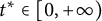 $t^* \in [0,+\infty )$
such that
 $\lim _{n \rightarrow +\infty } t_n=t^*$
.
Lemma 2.4 [Reference Opial24]
Let C be a nonempty set of
 $\mathcal {H}$
and
 $\left \{t_n\right \}$
be a sequence in
 $\mathcal {H}$
. If
 $\lim _{n \rightarrow \infty }\left \|t_n-x\right \|$
exists for every
 $x \in C$
and every sequential weak cluster point of
 $\left \{t_n\right \}$
is in C, then
 $\left \{t_n\right \}$
converges weakly to a point in C.
Lemma 2.5 [Reference Saejung and Yotkaew25]
Let
 $\left \{t_n\right \}$
be a nonnegative sequence,
 $\left \{\sigma _n\right \}$
be a sequence of real numbers, and
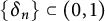 $\left \{\delta _n\right \}\subset (0,1)$
be a sequence such that
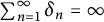 $\sum _{n=1}^{\infty } \delta _n=\infty $
. Assume that
 $$\begin{align*}t_{n+1} \leq\left(1-\delta_n\right) t_n+\delta_n \sigma_n, \quad \forall n \geq 1. \end{align*}$$
If
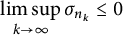 $\displaystyle \limsup _{k \rightarrow \infty } \sigma _{n_k} \leq 0$
for every subsequence
 $\left \{t_{n_k}\right \}$
of
 $\left \{t_n\right \}$
satisfying
 $\displaystyle \liminf _{k \rightarrow \infty } (t_{n_k+1}- t_{n_k} ) \geq 0$
, then
 $\lim _{n \rightarrow \infty } t_n=0$
.
3 Main results
In this section, we introduce two new iterative schemes based on the forward-backward-forward algorithm and the techniques of inertial and relaxation to solve the monotone inclusion problem. In the framework of real Hilbert spaces, the first proposed algorithm obtains weak convergence and
 $ R $
-linear convergence, while the second suggested algorithm can achieve strong convergence. Our algorithms directly improve on the results in [Reference Lorenz Pock1, Reference Boţ and Csetnek2, Reference Jolaoso, Shehu, Yao and Xu3, Reference Gibali and Thong17, Reference Thong, Cholamjiak, Pholasa, Dung and Long18] and many more.
3.1 Weak and linear convergence of Algorithm 3.1
The solution set of problem (1.1) is denoted as
 $ \mathrm {MIP}(A,B) $
. Before starting, we first assume that the proposed Algorithm 3.1 satisfies the following conditions.
-
(C1) The solution set of (1.1) is nonempty (i.e.,
). -
(C2) The operator
$A: \mathcal {H} \rightarrow \mathcal {H}$
is L-Lipschitz continuous and monotone, and the operator
$B: \mathcal {H} \rightarrow 2^{\mathcal {H}}$
is maximal monotone. -
(C3) Choose the parameters
$\eta \in (0,1)$
,
$\gamma \in [0,1)$
, and
$\sigma \in (0,1]$
satisfying the following condition: (3.1)
$$ \begin{align} \frac{\sigma(1-\eta^2)}{2-\sigma+\sigma\eta}(1-\gamma)^2-(1+\gamma) \gamma>0. \end{align} $$
 ).


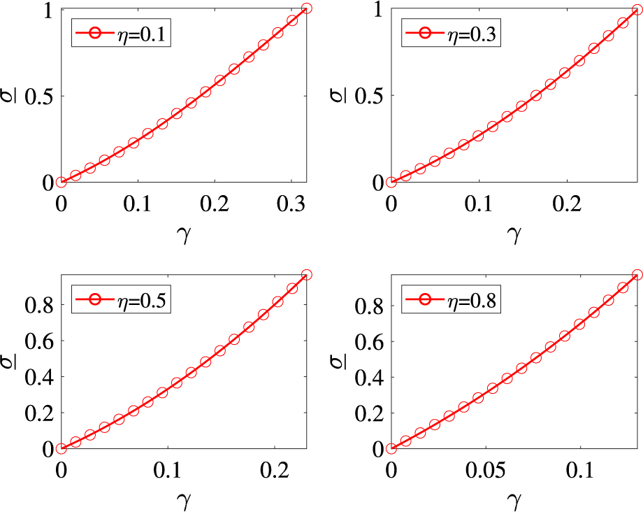
Remark 3.1 When the parameters
 $ \eta $
and
 $ \gamma $
are fixed, by solving Equation (3.1), we can obtain a lower bound on
 $ \sigma $
as

In other words, the parameter range of
 $ \sigma $
is
 $ \sigma \in (\underline {\sigma },1] $
when
 $ \eta $
and
 $ \gamma $
are fixed. Figure 1 gives the variation of
 $ \underline {\sigma } $
with
 $ \gamma $
when
 $ \eta $
is fixed.
The relationship between the parameters
 $ \gamma $
,
 $ \eta $
, and
 $ \underline {\sigma } $
.

We now proceed to present the proposed Algorithm 3.1.

The following lemmas are important for the convergence analysis of Algorithm 3.1.
Lemma 3.2 [Reference Tan, Petruşel, Qin and Yao26]
Suppose that Condition (C3) holds. Then the step size sequence
 $\left \{\psi _n\right \}$
created by (3.2) is well defined, and
 $\lim _{n \rightarrow \infty } \psi _n$
exists.
Lemma 3.3 [Reference Tan and Cho27]
Let the sequences
 $\left \{d_n\right \}$
and
 $\left \{g_n\right \}$
be generated by Algorithm 3.1. If
 $\lim _{n \rightarrow \infty } \| d_n-g_n \|=0$
and
 $\left \{d_{n_k}\right \}$
converges weakly to some
 $z \in \mathcal {H}$
, then
 $z \in \mathrm {MIP}(A,B)$
.
Theorem 3.4 (Weak convergence)
Suppose that Conditions (C1)–(C3) hold and let
 $\left \{t_n\right \}$
be any sequence formed by Algorithm 3.1. Then
 $\left \{t_n\right \}$
converges weakly to an
 $p \in \mathrm {MIP}(A,B)$
.
Proof Let
 $p \in \mathrm {MIP}(A,B)$
. From the definition of
 $ g_{n} $
, one has
 $\left (I-\psi _{n} A\right ) d_{n} \in \left (I+\psi _{n} B\right ) g_{n}$
. Since B is maximal monotone, there exists
 $v_{n} \in B g_{n}$
satisfying
 $ \left (I-\psi _{n} A\right ) d_{n}=g_{n}+\psi _{n} v_{n} $
. This is equivalent to
 $$ \begin{align} v_{n}=\psi_{n}^{-1}\left(d_{n}-g_{n}-\psi_{n} A d_{n}\right). \end{align} $$
We have
 $ (A+B) $
is maximal monotone by means of Condition (C2) and Lemma 2.2. This combined with
 $A g_{n}+v_{n} \in (A+B) g_{n} $
and
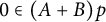 $0 \in (A+B) p$
implies that
 $ \langle A g_{n}+v_{n}, g_{n}-p \rangle \geq 0 $
, which together with (3.3) further yields
 $$ \begin{align} \left\langle d_{n}-g_{n}-\psi_{n}\left(A d_{n}-A g_{n}\right), g_{n}-p\right\rangle \geq 0. \end{align} $$
By the definition of
 $ u_{n} $
, one has
 $$ \begin{align} \begin{aligned} \left\|u_n-p\right\|^2 & = \left\|g_n-\psi_n\left(A g_n-A d_n\right)-p\right\|^2 \\ & = \left\|g_n-p\right\|^2+\psi_n^2\left\|A g_n-A d_n\right\|^2-2 \psi_n\left\langle g_n-p, A g_n-A d_n\right\rangle \\ & = \left\|d_n-p\right\|^2+\left\|d_n-g_n\right\|^2+2\left\langle g_n-d_n, d_n-p\right\rangle+\psi_n^2\left\|A g_n-A d_n\right\|^2 \\ & \quad-2 \psi_n\left\langle g_n-p, A g_n-A d_n\right\rangle \\ & = \left\|d_n-p\right\|^2+\left\|d_n-g_n\right\|^2-2\left\langle g_n-d_n, g_n-d_n\right\rangle+2\left\langle g_n-d_n, g_n-p\right\rangle \\ & \quad +\psi_n^2\left\|A g_n-A d_n\right\|^2-2 \psi_n\left\langle g_n-p, A g_n-A d_n\right\rangle \\ & = \left\|d_n-p\right\|^2-\left\|d_n-g_n\right\|^2-2\left\langle d_n-g_n-\psi_n\left(A d_n-A g_n\right), g_n-p\right\rangle \\ & \quad +\psi_n^2\left\|A g_n-A d_n\right\|^2. \end{aligned}\nonumber\\[-4pt] \end{align} $$
Using (3.2), (3.4), and (3.5), we have
 $$ \begin{align} \left\|u_n-p\right\|^2 \leq\left\|d_n-p\right\|^2-\left(1-\eta^2 \frac{\psi_n^2}{\psi_{n+1}^2}\right)\left\|d_n-g_n\right\|^2, \quad \forall p \in \mathrm{MIP}(A,B). \end{align} $$
It follows from the definition of
 $ t_{n} $
that
 $$ \begin{align} \begin{aligned} \left\|t_{n+1}-p\right\|^2 & =\left\|\left(1-\sigma\right)\left(d_n-p\right)+\sigma\left(u_n-p\right)\right\|^2 \\ & \leq\left(1-\sigma\right)\left\|d_n-p\right\|^2+\sigma\left\|u_n-p\right\|^2. \end{aligned} \end{align} $$
Substituting (3.6) into (3.7) gives
 $$ \begin{align} \left\|t_{n+1}-p\right\|^{2} \leq\left\|d_{n}-p\right\|^{2}-\sigma\left(1-\eta^2 \frac{\psi_n^2}{\psi_{n+1}^2}\right)\left\|d_{n}-g_{n}\right\|^{2}, \quad \forall p \in \mathrm{MIP}(A,B). \end{align} $$
From the definition of
 $u_n$
and (3.2), we obtain
 $$\begin{align*}\left\|u_n-g_n\right\| \leq \eta \frac{\psi_n}{\psi_{n+1}}\left\|d_n-g_n\right\|. \end{align*}$$
This together with the definition
 $ u_{n} $
yields
 $$ \begin{align} \begin{aligned} \left\|t_{n+1}-d_n\right\| & \leq\left\|t_{n+1}-g_n\right\|+\left\|d_n-g_n\right\| \\ & =\left\|(1-\sigma) (d_n-g_{n})+\sigma\left(u_n-g_n\right)\right\|+\left\|d_n-g_n\right\| \\ & \leq\left(2-\sigma+\sigma \eta \frac{\psi_n}{\psi_{n+1}}\right)\left\|d_n-g_n\right\|. \end{aligned} \end{align} $$
Substituting (3.9) into (3.8), we obtain
 $$ \begin{align} \left\|t_{n+1}-p\right\|^2 \leq\left\|d_n-p\right\|^2-\underbrace{\frac{\sigma\left(1-\eta^2 \frac{\psi_n^2}{\psi_{n+1}^2}\right)}{2-\sigma+\sigma \eta \frac{\psi_n}{\psi_{n+1}}}}_{\alpha_{n}}\left\|t_{n+1}-d_{n}\right\|^{2}. \end{align} $$
By the definition of
 $ d_{n} $
, one sees that
 $$ \begin{align} \begin{aligned} \left\|t_{n+1}-d_n\right\|^2 & =\left\|t_{n+1}-t_n-\gamma\left(t_n-t_{n-1}\right)\right\|^2 \\ & =\left\|t_{n+1}-t_n\right\|^2+\gamma^2\left\|t_n-t_{n-1}\right\|^2-2 \gamma\left\langle t_{n+1}-t_n, t_n-t_{n-1}\right\rangle \\ & \geq\left\|t_{n+1}-t_n\right\|^2+\gamma^2\left\|t_n-t_{n-1}\right\|^2-2 \gamma\left\|t_{n+1}-t_n\right\|\left\|t_n-t_{n-1}\right\| \\ & \geq\left(1-\gamma\right)\left\|t_{n+1}-t_n\right\|^2+\left(\gamma^2-\gamma\right)\left\|t_n-t_{n-1}\right\|^2. \end{aligned} \end{align} $$
Again using the definition of
 $ d_n $
, we have
 $$ \begin{align} \begin{aligned} \left\|d_n-p\right\|^2 & =\left\|t_n+\gamma\left(t_n-t_{n-1}\right)-p\right\|^2 \\ & =\left\|(1+\gamma)\left(t_n-p\right)-\gamma\left(t_{n-1}-p\right)\right\|^2 \\ & =(1+\gamma)\left\|t_n-p\right\|^2-\gamma\left\|t_{n-1}-p\right\|^2+\gamma(1+\gamma)\left\|t_n-t_{n-1}\right\|^2. \end{aligned} \end{align} $$
Putting (3.11) and (3.12) into (3.10), we obtain
 $$ \begin{align} \begin{aligned} \left\|t_{n+1}-p\right\|^2 & \leq(1+\gamma)\left\|t_n-p\right\|^2-\gamma\left\|t_{n-1}-p\right\|^2+\gamma(1+\gamma)\left\|t_n-t_{n-1}\right\|^2 \\ & \quad-\alpha_{n}\left(\left(1-\gamma\right)\left\|t_{n+1}-t_n\right\|^2+\left(\gamma^2-\gamma\right)\left\|t_n-t_{n-1}\right\|^2\right). \end{aligned} \end{align} $$
This implies that
 $$ \begin{align} \begin{aligned} & \left\|t_{n+1}-p\right\|^2- \gamma\left\|t_n-p\right\|^2+\left[\left(1+\gamma\right) \gamma-\alpha_{n}\left(\gamma^2-\gamma\right)\right]\left\|t_{n+1}-t_n\right\|^2 \\& \quad \leq \left\|t_n-p\right\|^2-\gamma\left\|t_{n-1}-p\right\|^2 +\left[\left(1+\gamma\right) \gamma-\alpha_{n}\left(\gamma^2-\gamma\right)\right]\left\|t_n-t_{n-1}\right\|^2 \\& \qquad -\left[\alpha_{n}\left(1-\gamma\right)-\left(1+\gamma\right) \gamma+\alpha_{n}\left(\gamma^2-\gamma\right)\right]\left\|t_{n+1}-t_n\right\|^2. \end{aligned} \end{align} $$
Let

and

From (3.14), one has
 $$ \begin{align*} \Delta_{n+1}-\Delta_n \leq-\epsilon_{n}\left\|t_{n+1}-t_n\right\|^2. \end{align*} $$
Note that
 $\lim _{n \rightarrow \infty } \epsilon _{n}>0 $
by Condition (3.1). This means that
 $\left \{\Delta _n\right \}$
is nonincreasing for all
 $n \geq 1$
. From
 $\lim _{n \rightarrow \infty }\left (1-\eta ^2 \frac {\psi _n^2}{\psi _{n+1}^2}\right )=1-\eta ^2>0$
, there exists
 $ \epsilon>0 $
and
 $N_{1} \in \mathbb {N}$
such that
 $\epsilon _{n}>\epsilon $
for all
 $n \geq N_{1}$
. Hence,
 $$ \begin{align} \Delta_{n+1}-\Delta_n \leq-\epsilon\left\|t_{n+1}-t_n\right\|^2, \quad \forall n\geq N_{1}. \end{align} $$
From
 $ \sigma \in (0,1] $
,
 $ \eta \in (0,1) $
, and
 $ \lim _{n \rightarrow \infty } \psi _{n} $
exists, one obtains that
 $ \alpha _{n} $
as defined in (3.10) is greater than
 $ 0 $
for all
 $ n\geq N_1 $
. Since
 $ \gamma \in [0,1) $
, one can check that
 $$\begin{align*}\left(1+\gamma\right) \gamma-\alpha_{n}\left(\gamma^2-\gamma\right) \geq 0, \quad \forall n\geq N_{1}. \end{align*}$$
This together with the definition of
 $ \Delta _n $
implies that
 $$\begin{align*}\Delta_n\geq \left\|t_n-p\right\|^2-\gamma\left\|t_{n-1}-p\right\|^2. \end{align*}$$
By induction, we have
 $$ \begin{align} \begin{aligned} \left\|t_n-p\right\|^2 & \leq \gamma\left\|t_{n-1}-p\right\|^2+\Delta_n \\ & \leq \gamma\left\|t_{n-1}-p\right\|^2+\Delta_{N_{1}} \\ & \leq \cdots \\ & \leq \gamma^{n-N_{1}}\left\|t_{N_{1}}-p\right\|^2+\Delta_{N_{1}}\left(\gamma^{n-N_{1}-1}+\cdots+1\right) \\ & \leq \gamma^{n-N_{1}}\left\|t_{N_{1}}-p\right\|^2+\frac{\Delta_{N_{1}}}{1-\gamma}, \quad \forall n\geq N_{1}. \end{aligned} \end{align} $$
It follows from the definition of
 $ \Delta _{n+1} $
that
 $$ \begin{align} \Delta_{n+1}\geq -\gamma\left\|t_n-p\right\|^2, \quad \forall n\geq N_{1}. \end{align} $$
By using (3.16) and (3.17), we obtain
 $$\begin{align*}-\Delta_{n+1} \leq \gamma\left\|t_n-p\right\|^2 \leq \gamma^{n-N_{1}+1}\left\|t_{N_{1}}-p\right\|^2+\frac{\gamma \Delta_{N_{1}}}{1-\gamma}. \end{align*}$$
This together with (3.15) further yields (noting that
 $ \gamma \in [0,1) $
)
 $$\begin{align*}\begin{aligned} \epsilon \sum_{n=N_{1}}^k\left\|t_{n+1}-t_n\right\|^2 & \leq \Delta_{N_{1}}-\Delta_{k+1} \\ & \leq \gamma^{k-N_{1}+1}\left\|t_{N_{1}}-p\right\|^2+\frac{\Delta_{N_{1}}}{1-\gamma} \\ & \leq\left\|t_{N_{1}}-p\right\|^2+\frac{\Delta_{N_{1}}}{1-\gamma}, \quad \forall k>N_{1}. \end{aligned} \end{align*}$$
This implies
 $\sum _{n=1}^{\infty }\left \|t_{n+1}-t_n\right \|^2<+\infty $
. Therefore, we obtain
 $$ \begin{align} \lim_{n \rightarrow \infty}\left\|t_{n+1}-t_n\right\| = 0. \end{align} $$
By the definition of
 $ d_{n} $
, one sees that
 $$\begin{align*}\left\|t_{n+1}-d_n\right\|^2=\left\|t_{n+1}-t_n\right\|^2+\gamma^2\left\|t_n-t_{n-1}\right\|^2-2 \gamma\left\langle t_{n+1}-t_n, t_n-t_{n-1}\right\rangle. \end{align*}$$
This combined with (3.18) gives
 $$ \begin{align} \lim_{n \rightarrow \infty} \left\|t_{n+1}-d_n\right\| = 0, \quad \lim_{n \rightarrow \infty}\left\|d_n-t_n\right\|=0. \end{align} $$
From (3.13), we obtain
 $$ \begin{align} \begin{aligned} \left\|t_{n+1}-p\right\|^2 & \leq \left\|t_n-p\right\|^2+\gamma\left(\left\|t_n-p\right\|^2-\left\|t_{n-1}-p\right\|^2\right) \\ & \quad+\left(\gamma(1+\gamma)-\alpha_{n}\left(\gamma^2-\gamma\right)\right)\left\|t_n-t_{n-1}\right\|^2. \end{aligned} \end{align} $$
Using
 $ \gamma \in (0,1) $
,
 $\sum _{n=1}^{\infty }\left \|t_{n}-t_{n-1}\right \|^2<+\infty $
, (3.20), and Lemma 2.3, we deduce that
 $$ \begin{align} \lim_{n \rightarrow \infty}\left\|t_n-p\right\|^2=l. \end{align} $$
By (3.18), (3.19), and (3.21), we obtain
 $$ \begin{align} \lim_{n \rightarrow \infty}\left\|t_{n+1}-p\right\|^2=l, \quad \lim_{n \rightarrow \infty}\left\|d_n-p\right\|^2=l. \end{align} $$
From (3.8) and (3.22), we have
 $$ \begin{align} \lim_{n \rightarrow \infty}\left\|g_n-d_n\right\|=0. \end{align} $$
Since
 $\left \{t_n\right \}$
is a bounded sequence, there exists a subsequence
 $\left \{t_{n_k}\right \}$
of
 $\left \{t_n\right \}$
and
 $z \in \mathcal {H}$
such that
 $t_{n_k} \rightharpoonup z$
. By means of (3.19), one has
 $d_{n_k} \rightharpoonup z$
. Then it follows from (3.23) and Lemma 3.3 that
 $z \in \mathrm {MIP}(A,B)$
. Therefore, we proved that
-
(i) for every
$p \in \mathrm {MIP}(A,B)$
,
$\lim _{n \rightarrow \infty }\left \|t_n-p\right \|$
exists (see (3.21)); -
(ii) every sequential weak cluster point of
$\left \{t_n\right \}$
is in
$\mathrm {MIP}(A,B)$
.




In the light of Lemma 2.4, one concludes that the sequence
 $\left \{t_n\right \}$
converges weakly to
 $p \in \mathrm {MIP}(A,B)$
, as desired.
Next, we show the
 $ R $
-linear convergence of Algorithm 3.1 in the case where the multi-valued operator involved is strongly monotone.
Theorem 3.5 (Linear convergence)
Let p be the unique solution and the sequence
 $\left \{t_n\right \}$
be generated by Algorithm 3.2. Assume that Conditions (C1) and (C2)
 $ ^{\prime } $
hold.
-
(C2)′ The operator
$A: \mathcal {H} \rightarrow \mathcal {H}$
is L-Lipschitz continuous and monotone, and the operator
$B: \mathcal {H} \rightarrow 2^{\mathcal {H}}$
is
$\mu $
-strongly monotone.


Choose
 $\eta \in (0,1)$
,
 $ \sigma \in (0,1] $
,
 $ \gamma \in [0,1) $
, and
 $ \xi \in (0,1) $
such that
 $$ \begin{align} 0 \leq \gamma \leq \frac{\omega\epsilon}{\omega\epsilon+2\omega+\epsilon}, \end{align} $$
where
 $ \omega $
and
 $ \epsilon $
are defined in (3.30). Then
 $\left \{t_n\right \}$
converges to the solution p of the problem (1.1) with an
 $ R $
-linear rate.
Proof Let
 $ p \in \mathrm {MIP}(A,B)$
. It follows from
 $g_n=\left (I+\psi _n B\right )^{-1}(I-\psi _n A) d_n$
that
 $\left (I-\psi _n A\right ) d_n \in \left (I+\psi _n B\right ) g_n$
. Hence,
 $$\begin{align*}\psi_n^{-1}(d_n-g_n-\psi_n A d_n) \in B g_n. \end{align*}$$
Since
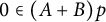 $ 0\in (A+B)p $
, one has
 $- A p \in B p$
. Using the fact that B is
 $\mu $
-strongly monotone, we have
 $$\begin{align*}\left\langle d_n-g_n-\psi_n A d_n+\psi_n A p, g_n-p\right\rangle \geq \mu\psi_{n}\left\|g_n-p\right\|^2. \end{align*}$$
This combined with the monotonicity of A implies
 $$ \begin{align} \begin{aligned} \left\langle d_n-g_n-\psi_n\left(A d_n-A g_n\right), g_n-p\right\rangle & \geq \mu\psi_{n}\left\|g_n-p\right\|^2+\psi_n\left\langle A g_n-A p, g_n-p\right\rangle \\ & \geq \mu\psi_n \left\|g_n-p\right\|^2. \end{aligned} \end{align} $$
By using (3.5), (3.7), and (3.25), we have
 $$ \begin{align} \begin{aligned} & \quad\left\|t_{n+1}-p\right\|^2 \\ &\leq\left\|d_n-p\right\|^2-\sigma\left(1-\eta^2 \frac{\psi_n^2}{\psi_{n+1}^2}\right)\left\|d_{n}-g_{n}\right\|^{2}-2\sigma \mu \psi_n \left\|g_n-p\right\|^2\\ &=\left\|d_n-p\right\|^2-\sigma(1-\xi)\left(1-\eta^2 \frac{\psi_n^2}{\psi_{n+1}^2}\right)\left\|d_{n}-g_{n}\right\|^{2}\\ &\quad-\sigma\xi\left(1-\eta^2 \frac{\psi_n^2}{\psi_{n+1}^2}\right)\left\|d_{n}-g_{n}\right\|^{2}-2\sigma \mu \psi_n \left\|g_n-p\right\|^2. \end{aligned} \end{align} $$
By means of (3.9), one sees that
 $$ \begin{align} \frac{1}{2-\sigma+\sigma \eta \frac{\psi_n}{\psi_{n+1}}}\left\|t_{n+1}-d_n\right\|\leq \left\|d_n-g_n\right\|. \end{align} $$
From (3.26) and (3.27), one has
 $$ \begin{align} \begin{aligned} \left\|t_{n+1}-p\right\|^2 & \leq \left\|d_n-p\right\|^2-\frac{\sigma(1-\xi)\left(1-\eta^2 \frac{\psi_n^2}{\psi_{n+1}^2}\right)}{\left(2-\sigma+\sigma \eta \frac{\psi_n}{\psi_{n+1}}\right)^2}\left\|t_{n+1}-d_{n}\right\|^{2}\\ & \quad-\sigma\xi\left(1-\eta^2 \frac{\psi_n^2}{\psi_{n+1}^2}\right)\left\|d_{n}-g_{n}\right\|^{2}-2\sigma \mu \psi_n \left\|g_n-p\right\|^2. \end{aligned} \end{align} $$
Let

Note that
 $ \delta \in (0,1) $
by means of (3.29),
 $ \sigma \in (0,1)$
,
 $ \xi \in (0,1) $
, and
 $ \eta \in (0,1) $
. Then we obtain

Thus, there exists
 $N \in \mathbb {N}$
such that
 $$\begin{align*}\frac{\sigma(1-\xi)\left(1-\eta^2 \frac{\psi_n^2}{\psi_{n+1}^2}\right)}{\left(2-\sigma+\sigma \eta \frac{\psi_n}{\psi_{n+1}}\right)^2}\geq \epsilon, \quad \sigma\xi\left(1-\eta^2 \frac{\psi_n^2}{\psi_{n+1}^2}\right)\geq 2\delta, \quad \sigma \mu \psi_n\geq \delta, \quad \forall n \geq N. \end{align*}$$
Let

Since
 $ \xi \in (0,1) $
,
 $ \eta \in (0,1) $
, and
 $ \sigma \in (0,1] $
, we have
 $ \omega \in (0,1) $
and
 $ \epsilon \in (0,1) $
. Using (3.27), we obtain
 $$\begin{align*}\begin{aligned} \left\|t_{n+1}-p\right\|^2 & \leq\left\|d_n-p\right\|^2-\epsilon\left\|t_{n+1}-d_n\right\|^2-2 \delta\left(\left\|d_n-g_n\right\|^2+\left\|g_n-p\right\|^2\right) \\ & \leq\left\|d_n-p\right\|^2-\epsilon\left\|t_{n+1}-d_n\right\|^2-\delta\left\|d_n-p\right\|^2. \end{aligned} \end{align*}$$
That is,
 $$ \begin{align} \left\|t_{n+1}-p\right\|^2 \leq \omega\left\|d_n-p\right\|^2-\epsilon\left\|t_{n+1}-d_n\right\|^2, \quad \forall n \geq N. \end{align} $$
From (3.11), (3.12), and (3.31), we deduce that
 $$\begin{align*}\begin{aligned} \left\|t_{n+1}-p\right\|^2 & \leq \omega\left(1+\gamma\right)\left\|t_n-p\right\|^2-\omega \gamma\left\|t_{n-1}-p\right\|^2+\omega \gamma\left(1+\gamma\right)\left\|t_n-t_{n-1}\right\|^2 \\ & \quad -\epsilon\left(1-\gamma\right)\left\|t_{n+1}-t_n\right\|^2+\epsilon \gamma\left(1-\gamma\right)\left\|t_n-t_{n-1}\right\|^2, \quad \forall n \geq N. \end{aligned} \end{align*}$$
This is equivalent to
 $$\begin{align*}\begin{aligned} & \left\|t_{n+1}-p\right\|^2-\omega \gamma\left\|t_n-p\right\|^2 +\epsilon\left(1-\gamma\right)\left\|t_{n+1}-t_n\right\|^2 \\ & \quad\leq \omega\left[\left\|t_n-p\right\|^2-\gamma\left\|t_{n-1}-p\right\|^2+\epsilon\left(1-\gamma\right)\left\|t_n-t_{n-1}\right\|^2\right] \\ & \qquad -\left(\omega \epsilon\left(1-\gamma\right)-\omega \gamma\left(1+\gamma\right)-\epsilon \gamma\left(1-\gamma\right)\right)\left\|t_n-t_{n-1}\right\|^2,\quad \forall n \geq N. \end{aligned} \end{align*}$$
We set

Since
 $\omega \in (0,1)$
, we have
 $$\begin{align*}\begin{aligned} \Sigma_{n+1} & \leq\left\|t_{n+1}-p\right\|^2-\omega \gamma\left\|t_n-p\right\|^2+\epsilon\left(1-\gamma\right)\left\|t_{n+1}-t_n\right\|^2 \\ & \leq \omega \Sigma_n-\left(\omega \epsilon\left(1-\gamma\right)-\omega \gamma\left(1+\gamma\right)-\epsilon \gamma\left(1-\gamma\right)\right)\left\|t_n-t_{n-1}\right\|^2, \quad \forall n \geq N. \end{aligned} \end{align*}$$
Thanks to
 $ \gamma \in [0,1) $
and (3.24), we obtain
 $$\begin{align*}\omega \epsilon\left(1-\gamma\right)-\omega \gamma\left(1+\gamma\right)-\epsilon \gamma\left(1-\gamma\right)\geq \omega \epsilon\left(1-\gamma\right)-2\omega \gamma-\epsilon\gamma\geq 0. \end{align*}$$
This implies that
 $ \Sigma _{n+1} \leq \omega \Sigma _n$
for all
 $n \geq N $
. Now, we show that
 $\Sigma _n> 0$
for all
 $n\geq N$
. From (3.24), we have
 $$\begin{align*}\gamma\leq\frac{\omega\epsilon}{\omega\epsilon+2\omega+\epsilon}< \frac{\epsilon}{2+\epsilon}. \end{align*}$$
This yields
 $$\begin{align*}\frac{\epsilon\left(1-\gamma\right)}{2}-\gamma> 0. \end{align*}$$
Using the definition of
 $ \Sigma _n $
, we deduce that
 $$\begin{align*}\begin{aligned} \Sigma_n & =\left(1-\epsilon\left(1-\gamma\right)\right)\left\|t_n-p\right\|^2+\epsilon\left(1-\gamma\right)\left(\left\|t_n-p\right\|^2+\left\|t_n-t_{n-1}\right\|^2\right)-\gamma\left\|t_{n-1}-p\right\|^2 \\ & \geq\left(1-\epsilon\left(1-\gamma\right)\right)\left\|t_n-p\right\|^2+\left(\frac{\epsilon\left(1-\gamma\right)}{2}-\gamma\right)\left\|t_{n-1}-p\right\|^2 \\ & \geq\left(1-\epsilon\left(1-\gamma\right)\right)\left\|t_n-p\right\|^2> 0. \end{aligned} \end{align*}$$
Hence,
 $ \Sigma _{n+1} \leq \omega \Sigma _n \leq \cdots \leq \omega ^{n-N+1} \Sigma _N $
. That is,
 $$\begin{align*}\left\|t_n-p\right\|^2 \leq \frac{\Sigma_N}{\left(1-\epsilon\left(1-\gamma\right)\right)\omega^{N}} \omega^n. \end{align*}$$
This implies that
 $\left \{t_n\right \}$
converges R-linearly to p. This completes the proof.
3.2 Strong convergence of Algorithm 3.2
In this subsection, we present a strongly convergent version of the FBF algorithm. More precisely, the iterative scheme is shown in Algorithm 3.2.

Theorem 3.6 (Strong convergence)
Assume that Conditions (C1), (C2), and (C4) hold. Then any sequence
 $\left \{t_n\right \}$
created by Algorithm 3.2 converges strongly to an element
 $p \in \mathrm {MIP}(A,B)$
, where
 $p=P_{\mathrm {MIP}(A,B)}(0)$
.
-
(C4) Take
$\psi _1>0$
,
$\gamma>0$
,
$\eta \in (0,1)$
, and
$\sigma \in (0,1]$
. Let
$\left \{\epsilon _n\right \}$
and
$\left \{\delta _n\right \} \subset (0,1)$
be two positive sequences that satisfy (3.33)
$$ \begin{align} \lim_{n \rightarrow \infty} \delta_n=0,\;\; \sum_{n=1}^{\infty} \delta_n=\infty \;\text { and } \lim_{n \rightarrow \infty} \frac{\epsilon_n}{\delta_n}=0. \end{align} $$




Proof Using similar arguments as (3.3)–(3.8) in the proof of Theorem 3.4, we have
 $$ \begin{align} \left\|t_{n+1}-p\right\|^{2} \leq\left\|d_{n}-p\right\|^{2}-\sigma\left(1-\eta^2 \frac{\psi_n^2}{\psi_{n+1}^2}\right)\left\|d_{n}-g_{n}\right\|^{2}, \quad \forall p \in \mathrm{MIP}(A,B). \end{align} $$
By the definition of
 $ d_{n} $
, one has
 $$ \begin{align} \begin{aligned} \left\|d_n-p\right\| & =\left\|\left(1-\delta_n\right)\left(t_n+\gamma_n\left(t_n-t_{n-1}\right)\right)-p\right\| \\ & =\left\|\left(1-\delta_n\right)\left(t_n-p\right)+\left(1-\delta_n\right) \gamma_n\left(t_n-t_{n-1}\right)-\delta_n p\right\| \\ & \leq\left(1-\delta_n\right)\left\|t_n-p\right\|+\left(1-\delta_n\right) \gamma_n\left\|t_n-t_{n-1}\right\|+\delta_n\left\|p\right\| \\ & =\left(1-\delta_n\right)\left\|t_n-p\right\|+\delta_n\left[\left(1-\delta_n\right) \frac{\gamma_n}{\delta_n}\left\|t_n-t_{n-1}\right\|+\left\|p\right\|\right]. \end{aligned} \end{align} $$
From (3.32) and (3.33), we have
 $$\begin{align*}\frac{\gamma_n}{\delta_n}\left\|t_n-t_{n-1}\right\| \leq \frac{\epsilon_n}{\delta_n} \rightarrow 0 \text{ as } n \to \infty. \end{align*}$$
This follows that
 $\lim _{n \rightarrow \infty }\left [\left (1-\delta _n\right ) \frac {\gamma _n}{\delta _n}\left \|t_n-t_{n-1}\right \|+\left \|p\right \|\right ]=\left \|p\right \|$
; thus, there exists
 $M>0$
such that
 $$ \begin{align} \left(1-\delta_n\right) \frac{\gamma_n}{\delta_n}\left\|t_n-t_{n-1}\right\|+\left\|p\right\| \leq M, \quad \forall n\geq 1. \end{align} $$
Using (3.35) and (3.36), one gives that
 $$ \begin{align} \left\|d_n-p\right\| \leq\left(1-\delta_n\right)\left\|t_n-p\right\|+\delta_n M. \end{align} $$
Since
 $\lim _{n \rightarrow \infty }\left (1-\eta ^2 \frac {\psi _n^2}{\psi _{n+1}^2}\right )=1-\eta ^2>0$
, there exists
 $n_{0} \in \mathbb {N}$
such that
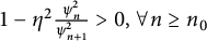 $1-\eta ^2 \frac {\psi _n^2}{\psi _{n+1}^2}>0, \forall n \geq n_{0}$
. This together with (3.34) yields that
 $$ \begin{align} \left\|t_{n+1}-p\right\| \leq\left\|d_n-p\right\|, \quad \forall n \geq n_0. \end{align} $$
By using (3.37) and (3.38), we obtain
 $$\begin{align*}\begin{aligned} \left\|t_{n+1}-p\right\| & \leq \left(1-\delta_n\right)\left\|t_n-p\right\|+\delta_n M \\ & \leq \max \left\{\left\|t_n-p\right\|, M\right\} \leq \cdots \leq \max \left\{\left\|t_{n_{0}}-p\right\|, M\right\}. \end{aligned} \end{align*}$$
This means that the sequence
 $\left \{t_n\right \}$
is bounded. Thus, the sequences
 $\left \{d_n\right \}$
,
 $\left \{g_n\right \}$
, and
 $\left \{u_n\right \}$
are also bounded by means of (3.37), (3.34), and (3.6).
From (3.37) and note that
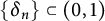 $\left \{\delta _n\right \} \subset (0,1)$
, one finds
 $$ \begin{align} \begin{aligned} \left\|d_n-p\right\|^2 & \leq\left(1-\delta_n\right)^2\left\|t_n-p\right\|^2+2 \delta_n\left(1-\delta_n\right) M\left\|t_n-p\right\|+\delta_n^2 M^2 \\ & \leq\left\|t_n-p\right\|^2+\delta_n M_1, \end{aligned} \end{align} $$
where  . Substituting (3.39) into (3.34), we have
 $$ \begin{align} \sigma\left(1-\eta^2 \frac{\psi_n^2}{\psi_{n+1}^2}\right)\left\|d_{n}-g_{n}\right\|^{2} \leq\left\|t_n-p\right\|^2-\left\|t_{n+1}-p\right\|^2+\delta_n M_1. \end{align} $$
Using the inequality (3.38) and the definition of
 $ d_{n} $
, we obtain
 $$\begin{align*}\begin{aligned} \left\|t_{n+1}-p\right\|^2 & \leq \left\|\left(1-\delta_n\right)\left(t_n-p\right)+\left(1-\delta_n\right) \gamma_n\left(t_n-t_{n-1}\right)-\delta_n p\right\|^2 \\ & \leq \left\|\left(1-\delta_n\right)\left(t_n-p\right)+\left(1-\delta_n\right) \gamma_n\left(t_n-t_{n-1}\right)\right\|^2+2 \delta_n\left\langle-p, d_n-p\right\rangle \\ & \leq \left(1-\delta_n\right)^2\left\|t_n-p\right\|^2+2\left(1-\delta_n\right) \gamma_n\left\|t_n-p\right\|\left\|t_n-t_{n-1}\right\| \\ & \quad +\gamma_n^2\left\|t_n-t_{n-1}\right\|^2+2\delta_n\left\langle-p, d_n-t_{n+1}\right\rangle+2\delta_n\left\langle-p, t_{n+1}-p\right\rangle. \end{aligned} \end{align*}$$
This yields that
 $$ \begin{align} \begin{aligned} & \left\|t_{n+1}-p\right\|^2 \\ &\quad\leq \left(1-\delta_n\right)\left\|t_n-p\right\|^2+\delta_n\left[2\left(1-\delta_n\right)\left\|t_n-p\right\| \frac{\gamma_n}{\delta_n}\left\|t_n-t_{n-1}\right\|\right. \\ &\qquad \left.+\gamma_n\left\|t_n-t_{n-1}\right\| \frac{\gamma_n}{\delta_n}\left\|t_n-t_{n-1}\right\|+2\left\|p\right\|\left\|d_n-t_{n+1}\right\|+2\left\langle p, p-t_{n+1}\right\rangle\right]. \end{aligned} \end{align} $$
Next, we show that
 $\left \{\left \|t_n-p\right \|\right \}$
converges to zero. Indeed, by Lemma 2.5, it suffices to prove that
 $ \lim \sup _{k \rightarrow \infty } \|d_{n_k}-t_{{n_k}+1}\|=0 $
and
 $\lim \sup _{k \rightarrow \infty }\langle p, p-t_{n_{k}+1}\rangle \leq 0$
for every subsequence
 $\left \{\|t_{n_k}-p\|\right \}$
of
 $\left \{\left \|t_n-p\right \|\right \}$
satisfying
 $$ \begin{align} \liminf _{k \rightarrow \infty}\left(\left\|t_{n_k+1}-p\right\|-\left\|t_{n_k}-p\right\|\right) \geq 0. \end{align} $$
For this, assume that
 $\left \{\|t_{n_k}-p\|\right \}$
is a subsequence of
 $\left \{\left \|t_n-p\right \|\right \}$
such that (3.42) holds. Then
 $$\begin{align*}\begin{aligned} & \liminf _{k \rightarrow \infty}\left(\left\|t_{n_k+1}-p\right\|^2-\left\|t_{n_k}-p\right\|^2\right) \\ & \quad =\liminf _{k \rightarrow \infty}\left[\left(\left\|t_{n_k+1}-p\right\|-\left\|t_{n_k}-p\right\|\right)\left(\left\|t_{n_k+1}-p\right\|+\left\|t_{n_k}-p\right\|\right)\right] \geq 0. \end{aligned} \end{align*}$$
By (3.40) and
 $ \lim _{n \rightarrow \infty } \delta _n=0 $
, we obtain
 $$\begin{align*}& \limsup _{k \rightarrow \infty} \sigma\left(1-\eta^2 \frac{\psi_{n_{k}}^2}{\psi_{n_{k}+1}^2}\right)\left\|d_{n_{k}}-g_{n_{k}}\right\|^{2} \\
& \quad \leq \limsup _{k \rightarrow \infty}\left[\left\|t_{n_k}-p\right\|^2-\left\|t_{n_k+1}-p\right\|^2+\delta_{n_k} M_1\right] \\
& \quad \leq \limsup _{k \rightarrow \infty}\left[\left\|t_{n_k}-p\right\|^2-\left\|t_{n_k+1}-p\right\|^2\right]+\limsup _{k \rightarrow \infty} \delta_{n_k} M_1 \\
& \quad =-\liminf _{k \rightarrow \infty}\left[\left\|t_{n_k+1}-p\right\|^2-\left\|t_{n_k}-p\right\|^2\right] \\& \quad \leq 0. \end{align*}$$
This implies that
 $$ \begin{align} \lim_{k \rightarrow \infty}\left\|g_{n_k}-d_{n_k}\right\|=0. \end{align} $$
From the definition of
 $u_n$
and (3.2), we obtain
 $$\begin{align*}\left\|u_{n_{k}}-g_{n_{k}}\right\| \leq \eta \frac{\psi_{n_{k}}}{\psi_{n_{k}+1}}\left\|d_{n_{k}}-g_{n_{k}}\right\|. \end{align*}$$
This combined with (3.43) yields that
 $$ \begin{align} \lim_{k \rightarrow \infty}\left\|u_{n_k}-g_{n_k}\right\|=0. \end{align} $$
By the definition of
 $ t_{n+1} $
, (3.43), and (3.44), we have
 $$ \begin{align} \lim_{k \rightarrow \infty}\left\|t_{n_k+1}-d_{n_k}\right\|=\lim_{k \rightarrow \infty} \sigma\left\|u_{n_k}-d_{n_k}\right\|=0. \end{align} $$
It follows from the definition of
 $ d_{n} $
that
 $$\begin{align*}\begin{aligned} \left\|t_{n_k}-d_{n_k}\right\| & =\left\|\left(1-\delta_{n_k}\right) \gamma_{n_k}\left(t_{n_k}-t_{n_k-1}\right)-\delta_{n_k} t_{n_k}\right\| \\ & \leq\delta_{n_k}\left[\left(1-\delta_{n_k}\right) \frac{\gamma_{n_k}}{\delta_{n_k}}\left\|t_{n_k}-t_{n_k-1}\right\|+\left\|t_{n_k}\right\|\right]. \end{aligned} \end{align*}$$
Therefore, we deduce that
 $$ \begin{align} \lim_{k \rightarrow \infty}\left\|t_{n_k}-d_{n_k}\right\|= 0. \end{align} $$
From (3.45) and (3.46), we obtain
 $$ \begin{align} \lim_{k \rightarrow \infty}\left\|t_{n_k+1}-t_{n_k}\right\| = 0. \end{align} $$
Since
 $\left \{t_{n_k}\right \}$
is bounded, there exists a subsequence
 $\{t_{n_{k_j}}\}$
of
 $\left \{t_{n_k}\right \}$
such that
 $\{t_{n_{k_j}}\}$
converges weakly to
 $z^*$
as
 $j \rightarrow \infty $
. Thanks to (3.46), one has
 $ d_{n_k} \rightharpoonup z^* $
. This combined with (3.43) and Lemma 3.3 implies that
 $ z^* \in \mathrm {MIP}(A,B) $
. By using the property of projection (cf. (2.1)) and the definition of
 $p=P_{\mathrm {MIP}(A,B)}(0)$
, we have
 $$ \begin{align} \limsup _{k \rightarrow \infty}\left\langle p, p-t_{n_k}\right\rangle=\lim_{j \rightarrow \infty}\langle p, p-t_{n_{k_{j}}}\rangle=\left\langle p, p-z^*\right\rangle \leq 0. \end{align} $$
From (3.47) and (3.48), one gives
 $$ \begin{align} \limsup _{k \rightarrow \infty}\left\langle p, p-t_{n_k+1}\right\rangle \leq 0. \end{align} $$
This together with (3.41), (3.45),
 $\lim _{n \rightarrow \infty } \frac {\gamma _n}{\delta _n}\left \|t_n-t_{n-1}\right \|=0$
, and Lemma 2.5 yields that
 $\lim _{n \rightarrow \infty }\left \|t_n-p\right \|=0$
. That is,
 $ t_n \rightarrow p $
as
 $ n\to \infty $
.
4 Numerical experiments
In this section, we apply the suggested Algorithms 3.1 and 3.2 to solve the signal recovery problem described in Example 1.1 and compare them with the ones in the literature [Reference Gibali and Thong17, Reference Thong, Cholamjiak, Pholasa, Dung and Long18]. All codes were executed in MATLAB 2018a on a personal computer with RAM 8.00 GB.
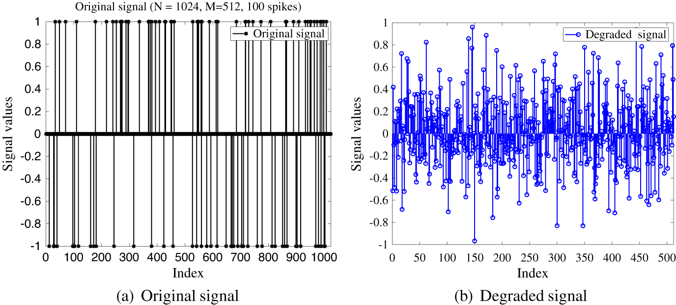
Original signal and degraded signal.

Example 4.1 (Signal Recovery Problem)
In our numerical experiments, the origin signal
 $\mathbf {x}$
is a vector of N values, where N is significantly greater than k, the number of randomly created spikes with either
 $+1$
or
 $-1$
. The matrix
 $\mathbf {C}$
with dimensions
 $M \times N$
is created using a standard normal distribution with a zero mean and unit variance, and its rows are then orthonormalized. We introduce white Gaussian noise with a variance of
 $10^{-4}$
, represented by
 $\epsilon $
, to generate the observation
 $\mathbf {y}$
using equation
 $\mathbf {y}=\mathbf {C} \mathbf {x}+\epsilon $
. The recovery procedure starts with the initial signals
 $\mathbf {t_{0}}$
and
 $\mathbf {t_{1}}$
set to zero and terminates after 100 iterations. The accuracy of the restoration is measured utilizing the mean squared error (MSE), which is calculated as
 $ \mathrm {MSE}=\frac {1}{N}\left \|\mathbf {x}^{*}-\mathbf {x}\right \|^{2}, $
where
 $\mathbf {x}^{*}$
is an estimated signal of the origin
 $\mathbf {x}$
and
 $ N $
denotes the dimension of
 $\mathbf {x}$
. The parameters of our algorithms and the compared ones are set as follows.
-
• Set
$ \psi _{1}=1 $
,
$ \eta =0.5 $
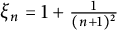
,
$ \xi _{n}=1+\frac {1}{(n+1)^2} $
, and
$ \tau _{n} = \frac {1}{n+1} $
for the proposed Algorithms 3.1 and 3.2. Choose
$ \gamma =0.2 $
and
$ \sigma =0.9 $
for our Algorithm 3.1. Take
$ \gamma =0.5 $
,
$ \sigma =0.9 $
,
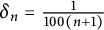
$ \delta _{n}=\frac {1}{100(n+1)} $
, and
$ \epsilon _n= \frac {1}{(n+1)^2}$
for our Algorithm 3.2. -
• Pick
$ \psi _{1}=1 $
,
$ \eta =0.5 $
,
$ \alpha _n=\frac {1}{n+1} $
, and
$ \delta _{n}=0.5(1-\alpha _n) $
for the Algorithm 1 proposed by Gibali and Thong [Reference Gibali and Thong17] (shortly, GT Alg. 1). Set
$ \psi _{1}=1 $
,
$ \eta =0.5 $
,
$ \alpha _n=\frac {1}{n+1} $
, and
$ f(x)=0.1x $
for the Algorithm 2 suggested by Gibali and Thong [Reference Gibali and Thong17] (shortly, GT Alg. 2) Take
$ \psi _{1}=1 $
,
$ \eta =0.5 $
,
$ \gamma =0.2 $
,
$ \sigma =0.4 $
, and
$ \tau _{n} = \frac {1}{n+1} $
for the Algorithm 1 introduced by Thong et al. [Reference Thong, Cholamjiak, Pholasa, Dung and Long18] (shortly, TCPDL Alg. 1).









In first test, we set
 $M=512$
,
 $N=1024$
, and
 $k=100$
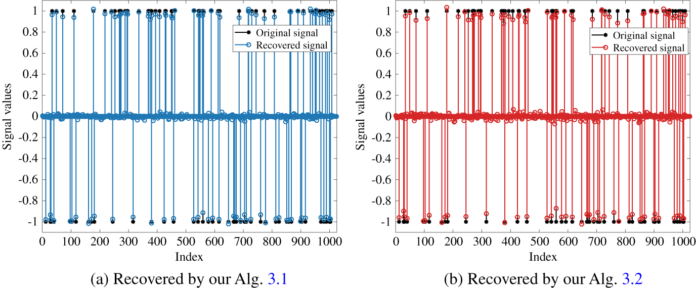
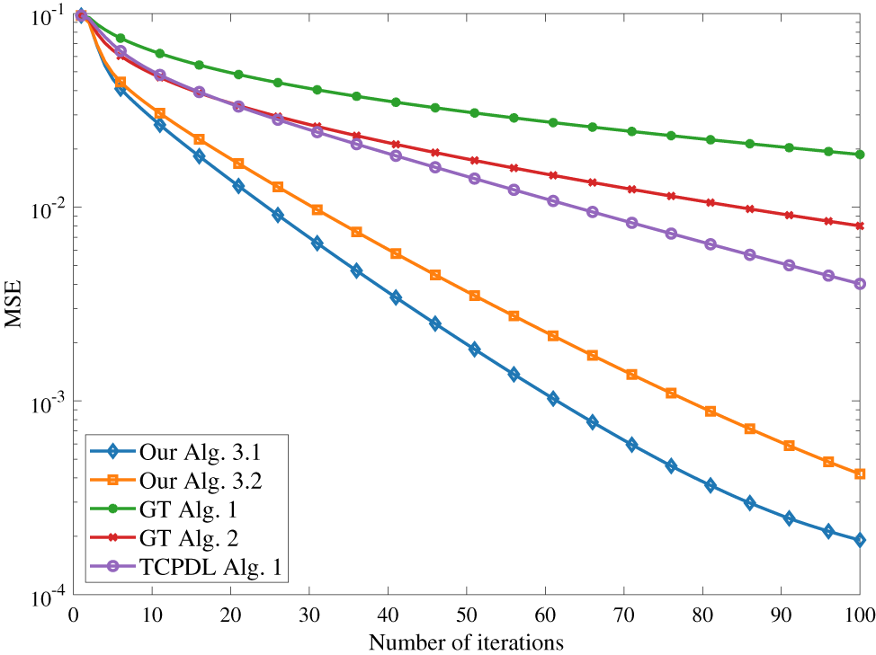
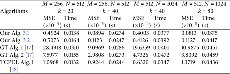
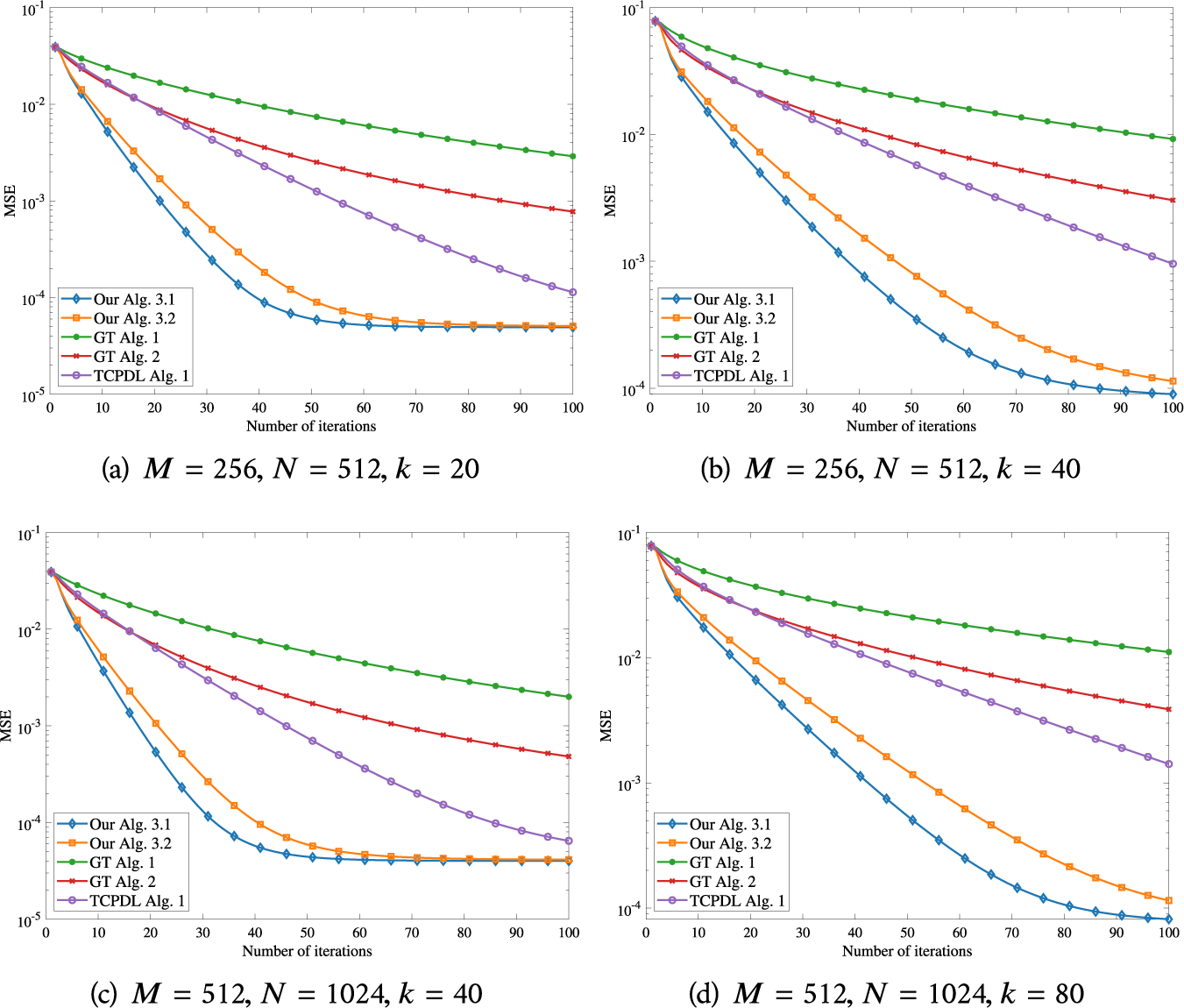
. The original and noisy signals are described in Figure 2, and the recovery results employing the proposed algorithms are shown in Figure 3. The variation of MSE with the number of iterations for all algorithms is stated in Figure 4. Finally, we applied all algorithms to solve the signal recovery problem under different dimensions and sparsity. The results are presented in Table 1 and Figure 5.
The original signal and the signal recovered by our algorithms.

The variation of MSE with the number of iterations for all algorithms at
 $ M=512, N=1024, k=100 $
.

The numerical results of all algorithms under different situations.

The variation of MSE with the number of iterations for all algorithms in four cases.

Remark 4.2 From Figures 2, 3, 4, and 5, and Table 1, it can be seen that the two algorithms proposed in this paper can effectively recover the original signal. Furthermore, the proposed algorithms perform better in terms of recovery as the original signal becomes sparser (i.e., when
 $ k \ll N $
). However, under the same dimensions and sparsity, the proposed algorithms converge faster and perform better than the algorithms in references [Reference Gibali and Thong17, Reference Thong, Cholamjiak, Pholasa, Dung and Long18].
5 Conclusions
The paper presents two novel algorithms that solve the monotone inclusion problem by incorporating improved forward-backward-forward methods with considerations of both the inertial term and the relaxation effect. Our results demonstrate that the proposed algorithms converge weakly and strongly, respectively, in real Hilbert spaces under suitable conditions. Furthermore, the first proposed algorithm is proven to have
 $ R $
-linear convergence when the multi-valued operator is strongly monotone. The suggested algorithms have been applied to signal recovery problems and have shown improved performance compared to previously published methods. These findings make a significant contribution to the field and open up new opportunities for further research.
Acknowledgements
The authors are very grateful to the editor and referees for their suggestions to help us improve the initial manuscript.