NOMENCLATURE

AR

aspect ratio

a _θ

circumferential inflow factor

a_ax

axial inflow factor

A ₁, A ₂, B ₁, B ₂

high angle-of-attack coefficients

B

number of propeller blades

BEMT

Blade Element Momentum Theory

c

propeller blade chord

C_d

drag coefficient

C _dmax

maximum drag coefficient

C _ds

stall drag coefficient

C_l

lift coefficient

C _lpot

lift coefficient from potential flow

C _lrot

lift coefficient due to rotation

C _{l non − rot}

lift coefficient without rotation

C _ls

stall lift coefficient

c_P

power coefficient

c_T

thrust coefficient

D

propeller diametre

dD

sectional drag force

dF _θ

sectional circumferential force

dL

sectional lift force

dr

sectional span

dT

sectional thrust force

dQ

sectional torque

J

advance ratio

K

velocity gradient

n

propeller rotational velocity (revolutions per second)

Q

torque

r

propeller blade radial position

R

maximum propeller blade radius

r_hub , r_tip

propeller hub and tip radial positions

$\overline{q}$

dynamic pressure

t

propeller sectional thickness

T

thrust

V_b

blade resultant velocity

V_i

induced velocity

V _∞

freestream velocity

V _θ

induced rotational velocity

V_ax

induced axial velocity

V_x

velocity in sectional x direction

V_z

velocity in sectional z direction

x

horizontal aerofoil axis

y

vertical aerofoil axis

Greek Symbols

α _b

blade angle-of-attack

α _s

stall angle

α _{C lmax}

angle-of-attack of maximum lift coefficient

α _{Cl = 0}

angle-of-attack of zero lift coefficient

β

aerodynamic pitch angle

$\frac{\partial C_{l}}{\partial \alpha }$

lift curve gradient

Δα

angle-of-attack shift

η

propeller efficiency

ε _b

blade downwash angle

ε _i

induced downwash angle

ε_∞

inflow angle

ω

angular velocity

ρ

air density

2.0 BLADE ELEMENT MOMENTUM THEORY

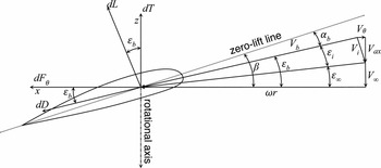
Blade element analysis models radially discretise the propeller blade into a number of elements. Each blade element can be considered as a rotating lifting surface, and it is assumed that the flow is two dimensional as seen in Fig. 1. Using this assumption, each element is considered to be independent of its ‘neighbour’ elements.

Figure 1.

Section forces and velocities acting on a rotating propeller blade^{(Reference Phillips29)}.

The blade is rotating with an angular velocity ω (n revolutions per second) and is advancing through the air with a relative airspeed V _∞. It is assumed that the forward velocity vector is aligned with the axis of propeller rotation such that no component of the forward airspeed is in the plane of rotation. The angle between the plane of rotation and the zero-lift line of the blade section is denoted by the aerodynamic pitch angle, β. Each propeller section has a different aerofoil section with its own unique zero lift line, and the geometric pitch must be adjusted for this difference.

The total downwash angle ε _b , for the blade element located at radius r is the sum of the downwash angle that results from the propeller’s forward motion, ε_∞ and the induced downwash angle, ε _i ,

(1) $$\begin{equation} \varepsilon _{b}(r) = \varepsilon _{\infty }(r) + \varepsilon _{i}(r) \end{equation}$$

In this paper, ε_∞ is called the advance angle, ε _i is called the induced angle, and ε _b is referred to as the blade downwash angle. Increasing blade downwash angle reduces the angle-of-attack for the aerofoil section and tilts the lift vector back, as shown in Fig. 1. This rotation of the lift vector through the angle ε _b increases the torque required to turn the propeller in much the same way that downwash adds induced drag to a lifting wing^{(Reference Phillips29)}.

The sectional thrust and circumferential forces can be found by applying a force balance to the blade element in both the axial and rotational directions:

(2) $$\begin{equation} dT & =& dL \cos {\varepsilon _{b}} - dD \sin {\varepsilon _{b}} \\ \end{equation}$$

(3) $$\begin{equation} dF_{\theta } & =& dL \sin {\varepsilon _{b}} + dD \cos {\varepsilon _{b}} \end{equation}$$

The advance angle of the blade ε_∞ is found by considering the blade axial and rotational velocity components:

(4) $$\begin{equation} \varepsilon _{\infty } = \tan ^{-1}\left(\frac{-V_{\infty }}{\omega r}\right) \end{equation}$$

As can be seen in Fig. 1, the induced velocity at the blade may be separated into an axial component V_ax and a circumferential component V _θ. The blade downwash angle then follows from:

(5) $$\begin{equation} \varepsilon _{b} = \tan ^{-1}\left(\frac{-(V_{\infty } + V_{ax})}{\omega r - V_{\theta }}\right) \end{equation}$$

Similarly, the velocity at the propeller blade is given by:

(6) $$\begin{equation} V_{b} = \sqrt{(-(V_{\infty } + V_{ax}))^{2} + (\omega r - V_{\theta })^{2} } \end{equation}$$

The local angle-of-attack at the blade element is found using the relation α _b = β − ε _b . This allows the local differential thrust and torque values to be calculated:

(7) $$\begin{equation} dT & =& \overline{q} \cdot c \cdot (C_{l} \cos {\varepsilon _{b}} - C_{d} \sin {\varepsilon _{b}}),\\ \end{equation}$$

(8) $$\begin{equation} dQ & =& \overline{q} \cdot c \cdot r \cdot (C_{l} \sin {\varepsilon _{b}} + C_{d} \cos {\varepsilon _{b}}), \end{equation}$$

where $\overline{q}$ describes the dynamic pressure at the blade element and is given by:

(9) $$\begin{equation} \overline{q} = \frac{1}{2} \cdot \rho \cdot V_{b}^{2} \end{equation}$$

The differential thrust and torque values are then integrated along the blade radius and across B blades as:

(10) $$\begin{equation} T = B \int _{r_{hub}}^{r_{tip}} dT dr \hspace{30.0pt} Q = B \int _{r_{hub}}^{r_{tip}} dQ dr \end{equation}$$

From the torque required to turn the propeller, the shaft power can be calculated using P = ωQ, and the dimensionless thrust and power coefficients are defined as:

(11) $$\begin{equation} c_{T} = \frac{T}{\rho n^{2} D^{4}} \hspace{30.0pt} c_{P} = \frac{P}{\rho n^{3} D^{5}}, \end{equation}$$

where D is the propeller diametre. The advance ratio and propeller efficiency are given by:

(12) $$\begin{equation} J = \frac{V_{\infty }}{n D} \hspace{30.0pt} \eta = \frac{c_{T}}{c_{P}} J \end{equation}$$

To calculate the induced velocities and hence the induced downwash angle, conservation of both axial and angular momentum is applied to each radial element of the blade. The axial and circumferential inflow factors a_ax and a _θ are defined as:

(13) $$\begin{equation} a_{ax} & =& \frac{V_{z} + V_{ax}}{V_{z}}, \\ \end{equation}$$

(14) $$\begin{equation} a_{\theta } & =& \frac{V_{x} - V_{\theta }}{V_{x}} \end{equation}$$

Applying the conservation of axial momentum to the streamtube swept out by each radial blade element leads to:

(15) $$\begin{equation} dT = 4 \pi r \cdot \rho \cdot V_{\infty }^{2} \cdot (1 + a_{ax}) \cdot dr \cdot a_{ax} \end{equation}$$

Applying the conservation of angular momentum in the same manner gives:

(16) $$\begin{equation} dQ = 4 \pi r^{2} \cdot \rho \cdot V_{\infty }^{2} \cdot V_{x} \cdot (1 + a_{ax}) \cdot dr \cdot a_{\theta } \end{equation}$$

Using Equations (15) and (16) in conjunction with Equations (7) and (8) allows the inflow factors a_ax and a _θ to be solved using an iterative process. To do so, the variation of lift and drag coefficients with angle-of-attack and Reynolds number must be known. Providing accurate aerodynamic data to the blade element method is therefore crucial.

3.0 AEROFOIL ANALYSIS

To generate an accurate aerodynamic database, 3D scanning is used to extract the aerofoil sections from the geometry of each propeller. Following this, the computer program XFOIL is used to obtain an aerodynamic polar, which is extended to post-stall angles of attack using either wind-tunnel data published by Ostowari and Naik^{(Reference Ostowari and Naik16)} or flat plate theory developed by Viterna and Corrigan^{(Reference Viterna and Corrigan17)}. The effects of rotation on aerodynamic coefficients are then simulated with either the Snel et al^{(Reference Snel, Houwink and Bosschers26)} 3D correction, or the stall delay method developed by Corrigan and Schillings^{(Reference Corrigan and Schillings27)}.

3.1 Propeller geometry

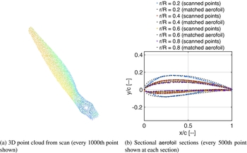
To extract the aerofoil sections that comprise a propeller blade, each of the tested propeller blades has been scanned using a David-3D^™ SLS-2 3D scanner. The process generates a high fidelity image of the complete blade geometry, as shown in Fig. 2(a).

Figure 2.

3D scan of an APC 19 × 12 Thin Electric propeller.

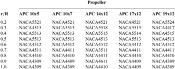
This allows accurate measurements of the propeller pitch, chord, and sectional aerodynamic shape at any radial position. By taking ‘slices’ along the blade radius, a number of aerofoils have been tabulated and used to represent each propeller. It was determined that the scanned point cloud at each radial position would be mapped to the closest fitting NACA four- or five-digit aerofoil section. NACA aerofoil profiles are generated internally in XFOIL, which ensures continuity of the higher order derivatives of the geometric shape of the aerofoil. This is necessary for convergence to sensible results at the low Reynolds numbers being investigated. This is consistent with the findings of Ol et al^{(Reference Ol, Zeune and Logan13)}. This process was completed using a least-squares fitting method. The results of this process are seen in Table 1.

Table 1

Propeller aerofoil sections

Aerodynamic data can then be found for each of the relevant aerofoils. Seen in Fig. 2(b), the aerofoil shape changes fairly significantly as a function of the blade radius.

3.2 Attached-flow aerodynamic analysis

The importance of appropriate aerofoil data for low Reynolds number applications has been well established in the analysis of small wind turbines^{(Reference Liller24,Reference Burdett, Gregg and Van Treuren30-Reference Van Treuren32)} , and the same holds true for small propellers^{(Reference Uhlig and Selig9,Reference Ol, Zeune and Logan13,Reference McCrink and Gregory23)} . When using blade element analysis methods, aerodynamic data is commonly obtained for a single Reynolds number, taken at 70–75% of the radius^{(Reference Viterna and Corrigan17,Reference Johnson33,Reference Tong34)} ; however, more recently, a number of analysis tools allowed use of aerodynamic data at various Reynolds numbers^{(Reference Morgado, Silvestre and Páscoa8,Reference Ol, Zeune and Logan13,Reference McCrink and Gregory23,Reference Liller24,Reference Drela35)} .

In this paper, an aerodynamic database has been constructed for a wide range of Reynolds numbers, allowing accurate representation of the flow for the appropriate conditions. At any blade section, the aerodynamic coefficients are obtained by interpolating with respect to both the local angle-of-attack and Reynolds number. The effects of Mach number are simulated using the Prandtl-Glauert correction applied at each blade section^{(Reference Leishman36)}. In this study, aerodynamic data is generated using XFOIL from a Reynolds number of 25,000 to 2,500,000. If the local Reynolds number is below the lower bound of 25,000, it is set to this value, and likewise for values above the upper bound.

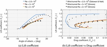
The variation of NACA 4412 aerodynamic coefficients with Reynolds number is shown in Fig. 3, obtained using the computer program XFOIL.^{(Reference Drela37)} XFOIL is an analysis and design panel code for low Reynolds number aerofoils, and is commonly used to provide aerodynamic data used in propeller and wind turbine analysis.^{(Reference Morgado, Silvestre and Páscoa8,Reference Ol, Zeune and Logan13,Reference Marten and Wendler21,Reference McCrink and Gregory23)}

Figure 3.

Aerodynamic data for the NACA 4412 aerofoil with varying Reynolds number (and wind-tunnel data obtained from Ostowari and Naik^{(Reference Ostowari and Naik16)} and Simons^{(Reference Simons44)}).

Examining Figs 3(a) and 3(b) shows that XFOIL slightly over-estimates the lift and drag for moderate Reynolds numbers (250,000). This is consistent with other findings, showing that XFOIL is able to replicate wind-tunnel data well down to a Reynolds number of 60,000–70,000^{(Reference Maughmer and Coder38,Reference Chen and Bernal39)} . At extremely low Reynolds numbers (20,000–30,000), XFOIL is seen to reproduce the wind-tunnel data presented by the Lnenicka test (see Borst^{(Reference Borst40)}) of a NACA 4412 aerofoil relatively well, although the lift curve slope is over-estimated and the drag under-estimated. However, the veracity of these results has been questioned, as no information was given about the tunnel or test conditions^{(Reference Borst40)}. This does not alleviate doubts about the accuracy of XFOIL at these Reynolds numbers as a result. Similar recommendations of caution were made by Ol et al^{(Reference Ol, Zeune and Logan13)} regarding the interpretation of both experimental and analytical aerodynamic data below Reynolds numbers of 60,000. Additionally, XFOIL is seen to struggle to accurately replicate aerofoil performance in the post-stall regime, and also suffers from accuracy degradation when simulating thick aerofoil performance^{(Reference van Rooij41-Reference Ramanujam and Özdemir43)}. These factors highlight the need for high quality low Reynolds number data across a suitable range of angles to validate the aerodynamic tools used to generate aerodynamic polars for small propeller analysis methods.

3.3 High angle-of-attack aerodynamic coefficients

A number of models have been developed to synthesise high angle-of-attack aerodynamic data, using wind-tunnel test data^{(Reference Critzos, Heyson and Boswinkle15,Reference Ostowari and Naik16)} , flat plate theory^{(Reference Viterna and Corrigan17)} and semi-empirical methods^{(Reference Montgomerie18-Reference Spera20)}. In this paper, the raw aerodynamic data generated using XFOIL has been extended using both flat plate theory^{(Reference Viterna and Corrigan17)} and wind-tunnel data for the NACA 4412 aerofoil^{(Reference Ostowari and Naik16)}.

Viterna and Corrigan^{(Reference Viterna and Corrigan17)} based their method on the idealised stall of an aerofoil. The model is characterised by the following expressions for the lift-and-drag coefficients:

(17) $$\begin{equation} C_{l}& =& A_{1} \sin (2 \alpha ) + A_{2} \frac{\cos ^{2}{\alpha }}{\sin {\alpha }},\\ \end{equation}$$

(18) $$\begin{equation} C_{d} & =& B_{1} \sin ^{2}(\alpha ) + B_{2} \cos {\alpha }, \end{equation}$$

where

(19) $$\begin{equation} A_{1} & =& \frac{B_{1}}{2}, \\ \end{equation}$$

(20) $$\begin{equation} B_{1} & =& C_{d_{max}} = 1.11 + 0.018AR,\\ \end{equation}$$

(21) $$\begin{equation} A_{2} & =& \left( C_{l_{s}} - C_{d_{max}} \sin {\alpha _{s}} \cos {\alpha _{s}}\right), \\ \end{equation}$$

(22) $$\begin{equation} B_{2} & =& C_{d_{s}} - \frac{C_{d_{s}} \sin ^{2}{\alpha _{s}}}{\cos {\alpha _{s}}} , \end{equation}$$

where the subscript s denotes that the above coefficients have been calculated using stall values to guarantee continuity with pre-stall data.

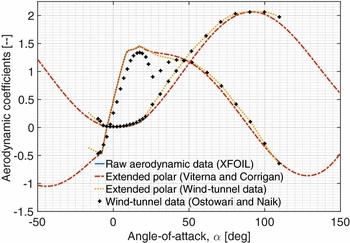
The extension of aerodynamic data to post-stall angles of attack can be seen in Fig. 4. A Reynolds number of 2.5 × 10⁵ is chosen to ensure a direct comparison can be made to available wind-tunnel data. This trend is continued in Fig. 5. When compared to wind-tunnel tests^{(Reference Ostowari and Naik16)}, at angles of attack greater than 45°, the Viterna and Corrigan^{(Reference Viterna and Corrigan17)} post-stall synthesis method reproduces lift coefficient fairly well. However, the model makes no attempt to reproduce the initial drop and recovery of the lift coefficient seen in test data. It has been suggested by Tangler and Ostowari^{(Reference Tangler and Ostowari10)} that this omission produces no significant error in the context of wind turbine analysis. However, this claim is contradicted by Timmer^{(Reference Timmer45)}, who concludes that data up to deep stall is required for accurate analysis of wind turbine performance. The availability of experimentally-obtained aerodynamic data, or lack thereof, is again a significant hurdle to evaluating these claims, especially in the context of small propeller analysis.

Figure 4.

NACA 4412 aerofoil data extended to high angles of attack (Re = 2.5 × 10⁵, AR = ∞) and windtunnel data^{(Reference Ostowari and Naik16)}.

Figure 5.

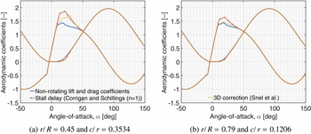
Rotating coefficients of a NACA 4412 section propeller (Re = 2.5 × 10⁵, AR = 15, V = 1 m/s, RPM = 3,000)

When considering drag, we can see that the post-stall drag coefficient produced by flat plate theory under-predicts drag by a substantial amount. Meanwhile, the most significant drawback of splining XFOIL polars to wind-tunnel results is the unavailability of wind-tunnel data points at negative angles of attack. It is particularly notable in Fig. 4 where the data is only available to –10^{o(Reference Ostowari and Naik16)}.

To account for aspect ratio and thickness effects, an alternate form of the maximum drag coefficient was formulated by Tangler and Ostowari^{(Reference Tangler and Ostowari10)}. This alternate form is around three times more sensitive to aspect ratio than the original formulation. Additionally, the alternate form was found to provide higher accuracy in lift modelling throughout the post stall region than the original form, with similar conclusions reached by Tangler and Ostowari^{(Reference Tangler and Ostowari10)}.

(23) $$\begin{equation} C_{d_{max}} = \frac{1 + 0.065AR}{0.9 + t/c} \end{equation}$$

3.4 Rotational effects

Propeller blades experience higher maximum lift coefficients and a delay of stall due to radial flow^{(Reference Himmelskamp25)}. This increase in maximum lift is more pronounced for blade sections located closer to the propeller hub^{(Reference Lindenburg19)}. In this paper, both the 3D correction developed by Snel et al^{(Reference Snel, Houwink and Bosschers26)} and the stall delay method formulated by Corrigan and Schillings^{(Reference Corrigan and Schillings27)} have been implemented to capture these rotational effects.

3.4.1 Snel et al model

The ‘3D correction method’ developed by Snel et al^{(Reference Snel, Houwink and Bosschers26)} is based on boundary-layer equations and models 3D flow effects due to rotation as an increase in the aerodynamic lift coefficient^{(Reference Snel, Houwink and Bosschers26)}. This correction has been applied to propeller performance prediction by Gur and Rosen^{(Reference Gur and Rosen7)}, and has found wide application in wind turbine prediction methods^{(Reference Lindenburg19,Reference Marten and Wendler21)} .

The Snel 3D correction is given by:

(24) $$\begin{equation} C_{l_{rot}} = C_{l_{non-rot}} + \tanh \left( 3.1 \cdot \left(\frac{\omega r}{V_{b}}\right)^{2} \cdot \left(\frac{c}{r}\right)^{2} \right) \cdot (C_{l_{pot}} - C_{l_{non-rot}}) \end{equation}$$

Due to the extremely high chord to radius ratios at the hub of small propellers, the following modification has been made to the correction model:

(25) $$\begin{equation} C_{l_{rot}} = C_{l_{non-rot}} + \frac{r}{R} \cdot \tanh \left( 3.1 \cdot \left(\frac{\omega r}{V_{b}}\right)^{2} \cdot \left(\frac{c}{r}\right)^{2} \right) \cdot (C_{l_{pot}} - C_{l_{non-rot}}) \end{equation}$$

The dependence on the relative radius term r/R ensures that the corrected lift coefficient remains realistic towards the blade root, while maintaining almost the full Snel 3D correction further along the blade.

The Snel 3D correction is applied from the zero-lift angle to an angle-of-attack of 30^o. From this point, the correction is decreased linearly to zero at 50^o, where it rejoins the originally extended aerofoil polar^{(Reference Lindenburg19)}.

3.4.2 Corrigan and Schillings model

Corrigan and Schillings^{(Reference Corrigan and Schillings27)} developed a model to correct for the effects of rotation on aerodynamic data whereby the stall of the aerofoil is delayed to higher angles of attack and the maximum lift coefficient is increased. The Corrigan and Schillings stall delay model was used by Morgado et al^{(Reference Morgado, Silvestre and Páscoa8)} and Uhlig and Selig^{(Reference Uhlig and Selig9)} to apply rotational corrections to propeller performance, showing tangible improvement over a generic method. The method has also seen extensive use in wind turbine analysis^{(Reference Lindenburg19,Reference Tangler and Selig28)} .

The Corrigan and Schillings model is based on a relation between the local blade chord to radius ratio (c/r), and the delay of stall is expressed with a shift in the angle-of-attack of the non-rotating coefficients:

(26) $$\begin{equation} \Delta \alpha = (\alpha _{C_{l_{max}}} - \alpha _{C_{l} = 0}) \cdot \left( \left(\frac{K (\frac{c}{r}) }{0.136} \right)^{n} - 1 \right), \end{equation}$$

where the velocity gradient K is related to the chord-to-radius ratio through

(27) $$\begin{equation} \left( \frac{c}{r}\right) = \frac{0.1517}{K^{1.084}} \end{equation}$$

A value of the exponent n between 0.8 and 1.6 gives a good correlation with most data^{(Reference Lindenburg19,Reference Corrigan and Schillings27,Reference Tangler and Selig28)} . In previous work^{(Reference Tangler and Selig28,Reference Xu and Sankar46)} , n = 1 was used as the value of the exponent, and this is continued in this paper.

In addition to the delay of stall, the lift coefficient is increased according to

(28) $$\begin{equation} C_{l_{rot}}(\alpha + \Delta \alpha ) = C_{l_{non-rot}}(\alpha + \Delta \alpha ) + \left( \frac{\partial C_{l}}{\partial \alpha } \right) \Delta \alpha , \end{equation}$$

where the gradient $\frac{\partial C_{l}}{\partial \alpha }$ is taken from the linear region of the lift-curve slope. The effects of the stall-delay model can be seen in Fig. 5.

In the implementation of both rotational methods, the drag values remain unmodified, as there are conflicting views about the effects of rotation on drag^{(Reference Lindenburg19)}. The stall delay method does however shift drag values to higher angles of attack, as seen in Fig. 5. Figure 5 also shows that the stall delay method exhibits increased lift augmentation compared to the 3D correction developed by Snel et al^{(Reference Snel, Houwink and Bosschers26)}. The effects of both methods decrease as the radius is increased (and the chord to radius ratio is reduced), though the 3D correction decreases in a far more pronounced manner.

The radial ‘suction’ due to centrifugal effects reduces significantly towards the free end of a rotating propeller blade. However, this radial flow from the inner part of the propeller blade produces a reduction in the negative pressure on the upper surface of the aerofoil compared to the non-rotating case. The lift coefficient of the tip region is then reduced to below the non-rotating lift value.

The reduction of lift coefficient in the tip region is described by an exponential function dependent on the aspect ratio of the blade outboard of the considered section: AR_out , following the model developed by Lindenburg^{(Reference Lindenburg19)}. The empirical formula is given by:

(29) $$\begin{equation} C_{l_{rot(tip)}} = C_{l_{non-rot}} - \left(\frac{\omega r}{V_{b}}\right)^{2} \cdot (C_{l_{pot}} - C_{l_{non-rot}}) \cdot \frac{C_{l_{non-rot}}}{C_{l_{pot}}} \end{equation}$$

The reduction in lift is a function of the ‘amount of stall’ captured with the term (C _lpot − C _{l non − rot} ), as well as the local speed ratio (ωr/V_b )², similar to the 3D correction method developed by Snel et al^{(Reference Snel, Houwink and Bosschers26)}. The reduction in lift is applied from radial sections outboard of 0.8r/R.

This effect is separate to the reduction in angle-of-attack resulting from airflow ‘leaking’ from the lower to the upper surface near the tip. The latter is due to the tip vortex and has been accounted for using Prandtl’s correction factor^{(Reference Lindenburg19,Reference Glauert47)} .

4.0 RESULTS AND ANALYSIS

To validate the accuracy of the developed method, as well as the effects of the implemented extensions, five test cases were selected. The APC Thin Electric 10 × 5, 10 × 7, 14 × 12, 17 × 12 and 19 × 12 propellers were selected to give a range of pitch and diametres, with experimental data available for each propeller^{(Reference Brandt48)}. Each of the test cases are model aircraft propellers, which routinely operate at low Reynolds numbers. The manufacturer lists that each propeller uses a series of aerofoils similar to Clark-Y and NACA 4412 sections⁽⁴⁹⁾; however, with the use of 3D scanning, the aerofoil sections that make up each propeller were extracted from the propeller geometry. The aerofoil sections found at a number of radial sections for each of the test propellers are shown in Table 1.

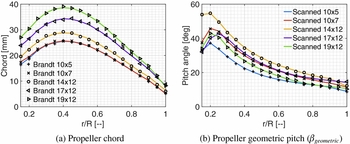
Using the characteristics shown in Fig. 6, the geometry of each propeller was recreated. Of particular difficulty was the validation of the geometric pitch distribution, as Brandt^{(Reference Brandt48)} does not give a clear indication of how pitch angle was recorded. After comparing the published data with that obtained from 3D scanning, it was found that the scanned geometric pitch angle was within 1.0° of the published pitch values^{(Reference Brandt48)}.

Figure 6.

Geometry of APC Thin Electric propellers^{(Reference Brandt48,49)} .

4.1 Validation of developed method

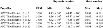
For each propeller, a number of simulations have been compared. A generic blade element momentum theory model is presented as a benchmark, using only a NACA 4412 section at a Reynolds number of 1 × 10⁶. Full Reynolds number dependency and geometrically accurate aerofoil sections have then been coupled with different combinations of high angle-of-attack and rotational methods. Finally, the extended BEMT has been examined with only a NACA 4412 section while allowing the Reynolds number to vary, and vice versa, to show the effect of each extension in turn. The range of Reynolds and Mach numbers faced by each propeller are tabulated in Table 2.

Table 2

Range of Reynolds and Mach numbers faced by tested propellers

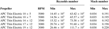
^a)The lower bound enforced on Reynolds number is 25 × 10³, while the upper bound is 2.5 × 10⁶.

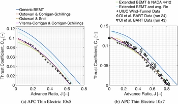
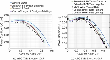
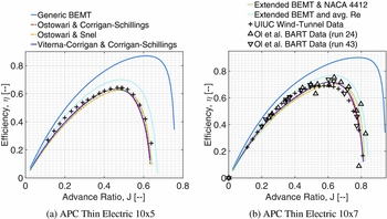
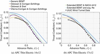
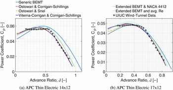
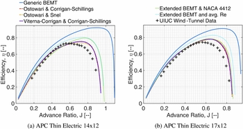
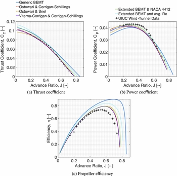
The simulation of the test propellers in Figs 7–9 and 11–14 exposes a number of common trends. The generic BEMT model over-estimates thrust coefficient at all advance ratios, consistently predicting values 30–40% above test data for smaller propellers, and 5–10% above for the 17 × 12 and 19 × 12 propellers. Power coefficient is over-estimated by the generic BEMT at high advance ratios, with the differences again 30–40% for the smaller propellers, and 5–10% for the 17 × 12 and 19 × 12 propellers. However, at low advance ratios, the opposite is true, which becomes more apparent for larger propellers, with under-predictions up to 10% when compared to test values. These differences combine to produce efficiency values around 35% and 20% larger than experimental data for small and large propellers, respectively.

Figure 7.

Thrust Coefficient of APC Thin Electric 10 × 5 and 10 × 7 propellers (5000 RPM)^{(Reference Ol, Zeune and Logan13,Reference Brandt48)} .

Figure 8.

Power Coefficient of APC Thin Electric 10 × 5 and 10 × 7 propellers (5000 RPM)^{(Reference Ol, Zeune and Logan13,Reference Brandt48)} .

Figure 9.

Propeller efficiency of APC Thin Electric 10 × 5 and 10 × 7 propellers (5000 RPM)^{(Reference Ol, Zeune and Logan13,Reference Brandt48)} .

Coupling the BEMT solution with the aerodynamic database extended using the techniques developed in this study significantly increases simulation accuracy. This is shown in the modelling of both thrust and power coefficients in Figs 7, 8, 11, 12 and 14, with a corresponding increase in the accuracy of efficiency modelling to within 5% of the experimental results at all advance ratios for smaller propellers, and within a maximum of 10% at the peak for larger (17 × 12 and 19 × 12) propellers.

Tests of the APC Thin Electric 10 × 7 propeller have also been conducted by Ol et al^{(Reference Ol, Zeune and Logan13)}; however, it must be noted that no RPM is specified in the published results. Good agreement is shown in Figs 7(b)–9(b) between the analysis method developed in this study and the test results published by both Ol et al^{(Reference Ol, Zeune and Logan13)} and Brandt^{(Reference Brandt48)}.

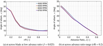
The extension of aerodynamic polars to high angles of attack with wind-tunnel data or the Viterna-Corrigan flat plate method produces similar results, with differences (at most less than 2%) seen only at low advance ratios. This is expected since blade sections face the highest angles of attack in this region, as shown in Fig. 10.

Figure 10.

Angle-of-attack distributions of APC Thin Electric 10 × 7 propeller.

The two different methods used to model rotational effects do however cause significant differences of around 5–10% in thrust and power coefficient modelling at low advance ratios. This is again expected as rotational effects are pronounced around the stall angle. The Snel et al^{(Reference Snel, Houwink and Bosschers26)} 3D correction produces lower thrust coefficients at low advance ratios than the Corrigan and Schillings^{(Reference Corrigan and Schillings27)} stall delay method due to its lower level of lift coefficient augmentation. This results in more accurate predictions for larger propellers, though for smaller propellers, the stall delay method is more precise.

Figure 7(b) and Figs 11(a) and 11(b) show that the BEMT method extended using flat plate theory^{(Reference Viterna and Corrigan17)} and stall delay^{(Reference Corrigan and Schillings27)} over-predicts thrust coefficient at low advance ratios. This can be linked to the high pitch angles of the 10 × 7, 14 × 12 and 17 × 12 propellers, shown in Fig. 6(b). For example, in the case of the 10 × 7 propeller, the inability of the extended BEMT method to accurately model power coefficient values at advance ratios below around 0.4 can be directly linked to angles of attack above 15° faced by the propeller sections, as seen in Fig. 10(b). This suggests an over-prediction of both lift and drag above 15° in the aerodynamic polars provided to the BEMT method. As mentioned earlier, this conclusion was also reached by Timmer^{(Reference Timmer45)}, and confirms the need for aerodynamic data through the angles of attack up to and beyond deep stall. The observations made by Tangler and Ostowari^{(Reference Tangler and Ostowari10)} are posited to not apply to the current investigation as significant changes in both lift curve slope and stall angle occur at low Reynolds numbers.

Figure 11.

Thrust Coefficient of APC Thin Electric 14 × 12 (3,500 RPM) and 17 × 12 propellers (3000 RPM)^{(Reference Brandt48)}.

Figure 12.

Power Coefficient of APC Thin Electric 14 × 12 (3,500 RPM) and 17 × 12 propellers (3,000 RPM)^{(Reference Brandt48)}.

Figure 13.

Propeller efficiency of APC Thin Electric 14 × 12 (3,500 RPM) and 17 × 12 propellers (3,000 RPM)^{(Reference Brandt48)}.

Figure 14.

Analysis of APC Thin Electric 19 × 12 propeller (3,000 RPM)^{(Reference Brandt48)}.

Meanwhile, all methods show over-prediction of power coefficient for both 10-inch diametre propellers (Figs 8(a) and 8(b)), suggesting the aerodynamic polars provided by XFOIL are less accurate due to the low Reynolds numbers. The relatively low chord values of these smaller propellers (Fig. 6(a)) result in lower Reynolds numbers. As the propeller size increases, simulated power coefficient values at low advance ratios increasingly under-predict the experimental values.

Again, referring to Fig. 10, at low advance ratios, the angles of attack towards the blade root are significantly above the stall angle. These trends do not change significantly with varying RPM (and as a consequence, varying Reynolds number). This suggests high angle-of-attack data produces the observed inaccuracies at low advance ratios. This is in line with previous findings where the inaccuracies at low advance ratios were attributed to possible misrepresentation of the aerofoil polar when extended to high angles of attack^{(Reference Morgado, Silvestre and Páscoa8)}. More specifically, this can be attributed to lower modelled drag figures than wind-tunnel values at high angles of attack, combined with over-estimated lift coefficient values in deep stall. It was noted that flat plate theory^{(Reference Viterna and Corrigan17)} produced an optimistic lift-to-drag ratio at high angles of attack^{(Reference Tangler and Ostowari10)}. This can be seen in Fig. 4 where lift and drag are slightly over- and under-predicted respectively, relative to wind-tunnel data. Additional uncertainty is introduced as the effect of rotation on aerodynamic drag is uncertain^{(Reference Lindenburg19)}.

When using the extended BEMT method with only a NACA 4412 section, the results are less accurate than with full aerofoil dependency, but the difference is less than may be expected. In the region of the propeller blade where the most thrust and power is produced (around 0.7–0.8(r/R)), each propeller has an aerofoil section similar to the NACA 4412 as shown in Table 1. This explains the relatively small difference observed. However, without prior knowledge of the aerofoil sections that make up a propeller, estimation of an aerofoil will often result in inaccurate aerodynamic data used for analysis.

When coupling the extended BEMT method with average Reynolds numbers for each blade section, both thrust and power coefficients are over-estimated throughout the advance ratio range, with increasing difference relative to experimental data as advance ratio is decreased. The differences observed in this case are around 15% and 25% for thrust and power coefficient, respectively, for smaller propellers, and similar inaccuracies to the generic BEMT are observed when simulating the performance of the 17 × 12 and 19 × 12 propellers. This can be attributed to the difference in aerodynamic coefficients using averaged as compared to fully variable Reynolds number data.

4.2 Impact of rotational speed

In the preceding section, a single RPM for each propeller has been considered. The ability to model performance at different rotational speeds is obviously important in the construction of a robust analysis method. This capability is verified in the following section.

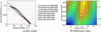
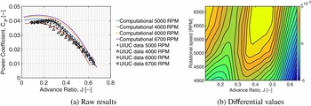
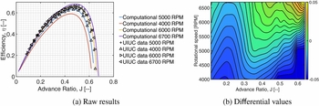
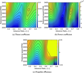
The variation of propeller performance with rotational speed is shown for the APC Thin Electric 10 × 5 in Figs 15(a)–17(a). This data is also represented as a difference between the extended BEMT model and experimental data in Figs 15(b)–17(b), and similarly for the APC Thin Electric 17 × 12 in Fig. 18. Visualising the difference between simulated and experimental data as contour levels clearly shows the regions of advance ratio where the extended BEMT is most (and least) accurate.

Figure 15.

Thrust coefficient of APC Thin Electric 10 × 5 propeller at varying RPM.

Figure 16.

Power coefficient of APC Thin Electric 10 × 5 propeller at varying RPM.

Figure 17.

Propeller efficiency of APC Thin Electric 10 × 5 propeller at varying RPM.

Figure 18.

Difference between computational and experimental data for APC Thin Electric 17 × 12.

Examining both Figs 15(b) and 18(a) more closely shows that at low advance ratios and low RPMs, simulated thrust coefficient values are lower than experimental data. This was also the case for the other tested propellers. The extremely low Reynolds numbers at this combination of low RPM and low advance ratios lead to this under-prediction, showing a pronounced need for accurate low Reynolds number aerodynamic data.

When simulating larger propellers, as shown in Fig. 18(b), the simulation of power coefficient also exhibits increasing inaccuracy at low advance ratios and with decreasing RPM. This phenomena can also be found in the simulation of the 14 × 12 and 19 × 12 propellers.

As seen in Fig. 16(b), the simulated power coefficient of the 10-inch diameter propellers becomes increasingly accurate with reducing RPM. However, for the larger propellers, computed power coefficient values diverge further from experimental values as the RPM is decreased. Again, this can be linked to the lack of quality low Reynolds number aerodynamic data.

For each test case, at the higher simulated RPM values, thrust and power coefficients are over-estimated at low advance ratios (though to a lesser extent with power coefficient of the 17 × 12 and 19 × 12 propellers). Contrary to the behaviour at low RPMs and therefore low Reynolds numbers, this suggests that high Reynolds number data produced by XFOIL results in overly optimistic lift-to-drag ratios. This is visually apparent in Fig. 3. These over-estimations are seen in the upper left regions of Figs 15(b)–17(b) and Fig. 18, and again in simulations of the other tested propellers.