1 Introduction
Contrary to conventional thought regarding fluid flow in porous media, a number of important applications exist wherein the Reynolds numbers can be so large that inertial effects become important and give rise to unsteady transitional and turbulent flows. Specific examples include catalysis in the chemical synthesis and process industries (Aris Reference Aris1969; Dixon & Nijemeisland Reference Dixon and Nijemeisland2001), high temperature nuclear reactor cooling (Shams et al. Reference Shams, Roelofs, Komen and Baglietto2013), hyporheic exchange of pollutants at the sediment–water interface (Hester et al. Reference Hester, Cardenas, Haggerty and Apte2017), and noise absorption and reduction at the trailing edges of airplane wings (Herr & Dobrzynski Reference Herr and Dobrzynski2005). In these examples, the contribution of the inertial terms can dramatically change the topology of the flow field leading to formation of jets, vortices, dead zones, etc., within the pores. Such flow features can substantially alter the dispersion characteristics of pollutants and play critical roles in the transport of reactants and products to and from active reaction sites.
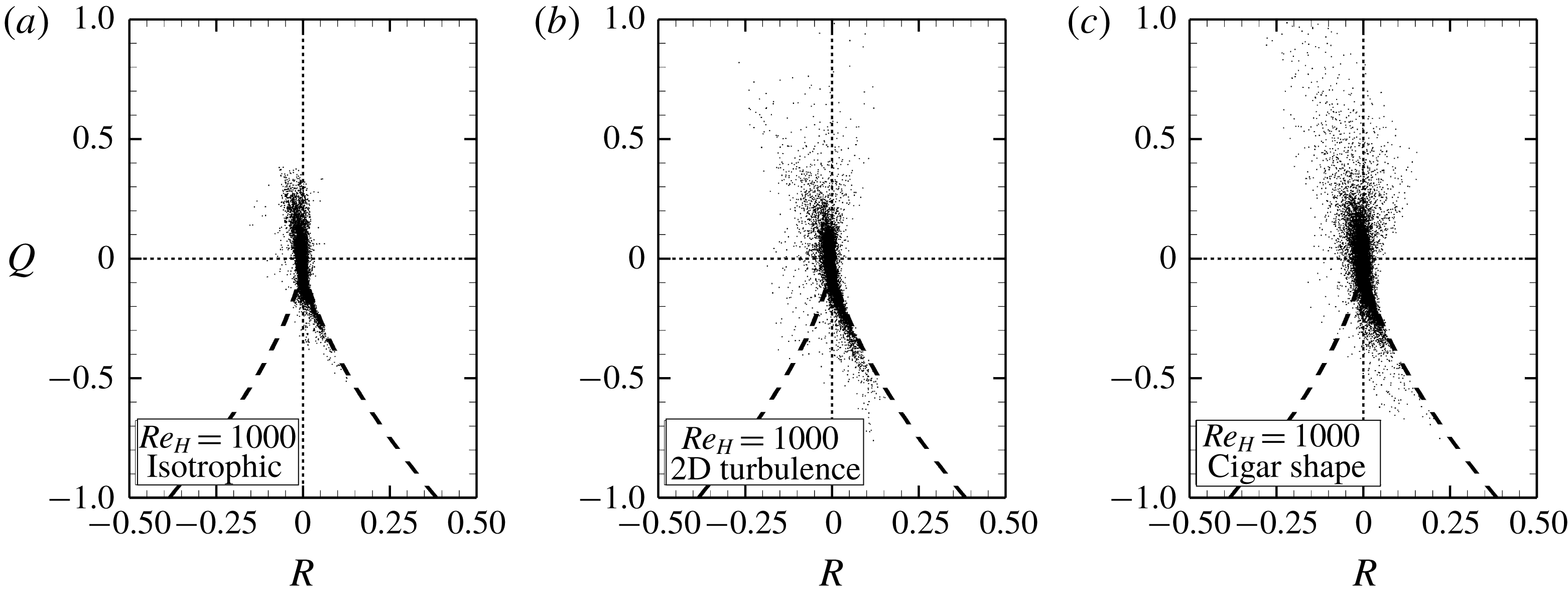
Several different definitions of Reynolds numbers have been used in the porous-media literature based on different length scales such as the particle diameter (
 $D_{B}$
), the hydraulic diameter (
 $D_{H}$
), or the permeability. In this work, Reynolds number (
 $Re_{H}$
) based on
 $D_{H}$
is used. The hydraulic diameter is related to the particle diameter as
 $$\begin{eqnarray}\displaystyle D_{H}=\frac{2}{3}\frac{\unicode[STIX]{x1D719}}{1-\unicode[STIX]{x1D719}}D_{B}. & & \displaystyle\end{eqnarray}$$
Then,
 $Re_{H}$
is defined as (dropping the factor
 $2/3$
)
 $$\begin{eqnarray}\displaystyle Re_{H}=\frac{\overline{\langle u_{x}\rangle ^{\unicode[STIX]{x1D6FE}}}D_{B}}{\unicode[STIX]{x1D708}_{\unicode[STIX]{x1D6FE}}}\frac{\unicode[STIX]{x1D719}}{1-\unicode[STIX]{x1D719}}, & & \displaystyle\end{eqnarray}$$
where
 $\unicode[STIX]{x1D708}_{\unicode[STIX]{x1D6FE}}$
is the kinematic viscosity of fluid,
 $\unicode[STIX]{x1D719}$
is the porosity of the medium defined as the ratio of the void volume to the total volume,
 $\overline{\langle u_{x}\rangle ^{\unicode[STIX]{x1D6FE}}}$
is the time-averaged interstitial (intrinsic average) velocity of flow in porous media, and
 $u_{x}$
is the instantaneous velocity component in the
 $x$
-(streamwise) direction. The spatial averaging operation is denoted by
 $\langle \,\cdot \,\rangle$
, the superscript
 $\unicode[STIX]{x1D6FE}$
indicates the fluid phase, and
 $\overline{~\cdot ~}$
is the time-averaging operator. For clarity, note that the intrinsic average velocity is defined by
 $$\begin{eqnarray}\displaystyle \langle u_{x}\rangle ^{\unicode[STIX]{x1D6FE}}|_{t}=\frac{1}{V_{\unicode[STIX]{x1D6FE}}}\int _{\boldsymbol{r}\in V_{\unicode[STIX]{x1D6FE}}}u_{x}(\boldsymbol{r},t)\,\text{d}V(\boldsymbol{r}), & & \displaystyle\end{eqnarray}$$
where
 $V_{\unicode[STIX]{x1D6FE}}$
is the volume of the fluid phase within the unit cell and the overbar represents traditional time-averaging defined as
 $$\begin{eqnarray}\displaystyle \overline{\unicode[STIX]{x1D713}}(t)=\frac{1}{T}\int _{t^{\ast }=t-T/2}^{t^{\ast }=t+T/2}\unicode[STIX]{x1D713}(t^{\ast })\,\text{d}t^{\ast }. & & \displaystyle\end{eqnarray}$$
Dybbs & Edwards (Reference Dybbs, Edwards, Bear and Corapcioglu1984) performed refractive-index-matched measurements in porous media to report on the topological characteristics of the pore-scale of the flow fields in the inertial range and classified the different flow regimes associated with Reynolds numbers as follows.
(i) Darcy or Creeping Flow Regime,
 $Re_{H}<10$
: Under these conditions, the flow is dominated by viscous forces. The drag force is proportional to the square of the Reynolds number, and contains negligible contributions from inertial forces (Hill, Koch & Ladd Reference Hill, Koch and Ladd2001).
(ii) The Steady Inertial (Nonlinear) Flow Regime,
 $10<Re_{H}<150$
: A dramatic change in the character of the flow has been observed to occur in this regime as inertial forces begin to dominate over viscous contributions (Natarajan & Acrivos Reference Natarajan and Acrivos1993; Suekane, Yokouchi & Hirai Reference Suekane, Yokouchi and Hirai2003). The influence of the inertial term on the resulting flow field in porous media is similar in many ways to the secondary flows that have been reported by Taylor and others for curved tubes (Taylor Reference Taylor1929; Roberts Reference Roberts2004). Helical vortices and other complex flows have been observed experimentally (Suekane et al.
Reference Suekane, Yokouchi and Hirai2003) and predicted numerically (Wegner, Karabelas & Hanratty Reference Wegner, Karabelas and Hanratty1971; Koch & Ladd Reference Koch and Ladd1997; Hill et al.
Reference Hill, Koch and Ladd2001; Wood Reference Wood2007; Finn Reference Finn2013) in simple periodic media at these Reynolds numbers.
(iii) Unsteady Laminar Flow Regime,
 $150<Re_{H}<350$
: In this regime, the flow is no longer steady (Wegner et al.
Reference Wegner, Karabelas and Hanratty1971), but it lacks the characteristics of a truly turbulent flow. Koch & Ladd (Reference Koch and Ladd1997) present 2-D numerical simulations in a regular array of cylinders that exhibit quasi-periodic vortex shedding. Also there have been direct experimental observations suggestive of vortex shedding (Mickley, Smith & Korchak Reference Mickley, Smith and Korchak1965; Van der Merwe & Gauvin Reference Van der Merwe and Gauvin1971; Latifi et al.
Reference Latifi, Midoux, Storck and Gence1989; Rode et al.
Reference Rode, Midoux, Latifi and Storck1994; Seguin, Montillet & Comiti Reference Seguin, Montillet and Comiti1998a
; Seguin et al.
Reference Seguin, Montillet, Comiti and Huet1998b
).
(iv) The Chaotic (Fully Developed Turbulence) Flow Regime,
 $Re_{H}>350+$
: Direct and indirect evidence of sub-pore-scale turbulence in porous media has been reported by several research groups (Hill & Koch Reference Hill and Koch2002; Finn Reference Finn2013; Finn & Apte Reference Finn and Apte2013; Patil & Liburdy Reference Patil and Liburdy2013, Reference Patil and Liburdy2015; Jin et al.
Reference Jin, Uth, Kuznetsov and Herwig2015; Uth et al.
Reference Uth, Jin, Kuznetsov and Herwig2016; Evseev Reference Evseev2017). There is some inconsistency among the groups, with some reporting turbulent conditions occurring at relatively low Reynolds numbers (
 $Re_{H}\sim 350+$
), whereas others have reported that turbulence was not observed until higher Reynolds numbers had been reached (
 $Re_{H}\sim 1000$
).
For high Reynolds number flows through porous media, answers to several fundamental questions related to the flow physics remain elusive. The pore-scale flow structure will no doubt change under the effects of stronger inertial contributions at higher Reynolds numbers. How this change of flow structure impacts the turbulence (i.e. the turbulent kinetic energy distribution and transport mechanisms) in the pore has not been thoroughly examined. Whether turbulence in a densely packed bed more closely resembles an internal duct flow or a separated external flow will have a bearing on the development of more accurate engineering models. The band-limiting caused by the confinement of the porous geometry is bound to alter the generation and transport of pore-scale turbulence, but to what extent is still unclear.
Although global measurements of pressure drop across a porous bed and longitudinal dispersion have been made for a range of Reynolds numbers leading to empirical correlations, such as Ergun equation and Darcy–Forchheimer law (Ergun Reference Ergun1952; Wen & Fan Reference Wen and Fan1975; Dixon & Cresswell Reference Dixon and Cresswell1986; Gunn Reference Gunn1987), detailed pore-scale investigations characterising the flow physics of transitional and turbulent flows in porous media are lacking (Hlushkou & Tallarek Reference Hlushkou and Tallarek2006). There have been very few comprehensive particle image velocimetry (PIV) investigations on pore-scale turbulent flows in porous media. Recently, Patil & Liburdy (Reference Patil and Liburdy2013, Reference Patil and Liburdy2015) measured the turbulent flow field up to
 $Re_{H}=4000$
using the two-component PIV method implementing the refractive-index-matching technique in a random packed bed. Evseev (Reference Evseev2017) used a similar approach to estimate the dispersion of turbulent flow in porous media. However, none of these studies were able to obtain fully-resolved, three-components of pore-scale velocity and pressure distributions over the entire volume of the porous bed. Thus, there is a lack of detailed flow data in complex configurations of porous geometries, and fully-resolved direct numerical studies become necessary to obtain these data. Such thorough flowfield results can then be used for developing and validating the Reynolds-averaged Navier–Stokes (RANS) models (Antohe & Lage Reference Antohe and Lage1997; Pedras & De Lemos Reference Pedras and De Lemos2001; Pearson & Tardy Reference Pearson and Tardy2002), as well as for closing the upscaled macroscopic volume-averaged equations (Masuoka & Takatsu Reference Masuoka and Takatsu1996; Nakayama & Kuwahara Reference Nakayama and Kuwahara1999; Whitaker Reference Whitaker1999; de Lemos & Pedras Reference de Lemos and Pedras2001; Suga Reference Suga2016).
Hill & Koch (Reference Hill and Koch2002) performed lattice Boltzmann simulations for flows through a close-packed ordered array of spheres to examine the steady and unsteady inertial flow regimes. The characteristics of flow transitioning to unsteady flow were quantified, but the fully turbulent flow regime was not explored. Some recent numerical works have conducted direct numerical simulations of turbulent flows in porous media, for example, Jin et al. (Reference Jin, Uth, Kuznetsov and Herwig2015), Uth et al. (Reference Uth, Jin, Kuznetsov and Herwig2016), Chu, Weigand & Vaikuntanathan (Reference Chu, Weigand and Vaikuntanathan2018). However, these authors mostly focused on the dilute porous systems with very large porosity (
 $0.5<\unicode[STIX]{x1D719}<0.9$
). Very few direct numerical simulation (DNS) studies for the densely-packed porous bed have been reported.
In this paper, we begin to address the lack of data for high-Reynolds-number flows in porous media by reporting on fully-resolved direct numerical simulations of flows in a closely-packed face-centred cubic lattice (cf. Hill & Koch Reference Hill and Koch2002) at Reynolds numbers ranging from the unsteady-inertial to fully-turbulent-flow regimes. The flow data are used to investigate the following questions.
(i) How does the local mean velocity structure within a pore influence the turbulence intensity, homogeneity and isotropicity?
(ii) What are the dominant mechanisms for turbulent energy production, dissipation and diffusion?
(iii) How does the flow topology and confined pore geometry influence the small scale velocity structures?
(iv) Can the Lagrangian time scale (and therefore the hydrodynamic dispersion) be characterized through the eddy length and turbulent velocity scales?
The remainder of paper is organized as follows. Section 2 provides the details of the geometry of the porous medium, the simulation parameters and the numerical methods. Computational results are presented in § 3; particular emphases are placed on the flow topology, the turbulent kinetic energy budget, anisotropy in the distribution of turbulent kinetic energy (TKE) and how the spatial confinement of a low porosity geometry affects turbulence structures. Finally, § 4 provides an overview of the results and reports the conclusions.
2 Computational geometry and numerical methodology
In this section, the computational geometry used in the current study is described, followed by a brief description of the numerical approach, grid resolution requirements, and corresponding grid refinement studies.
2.1 Geometry of the porous medium
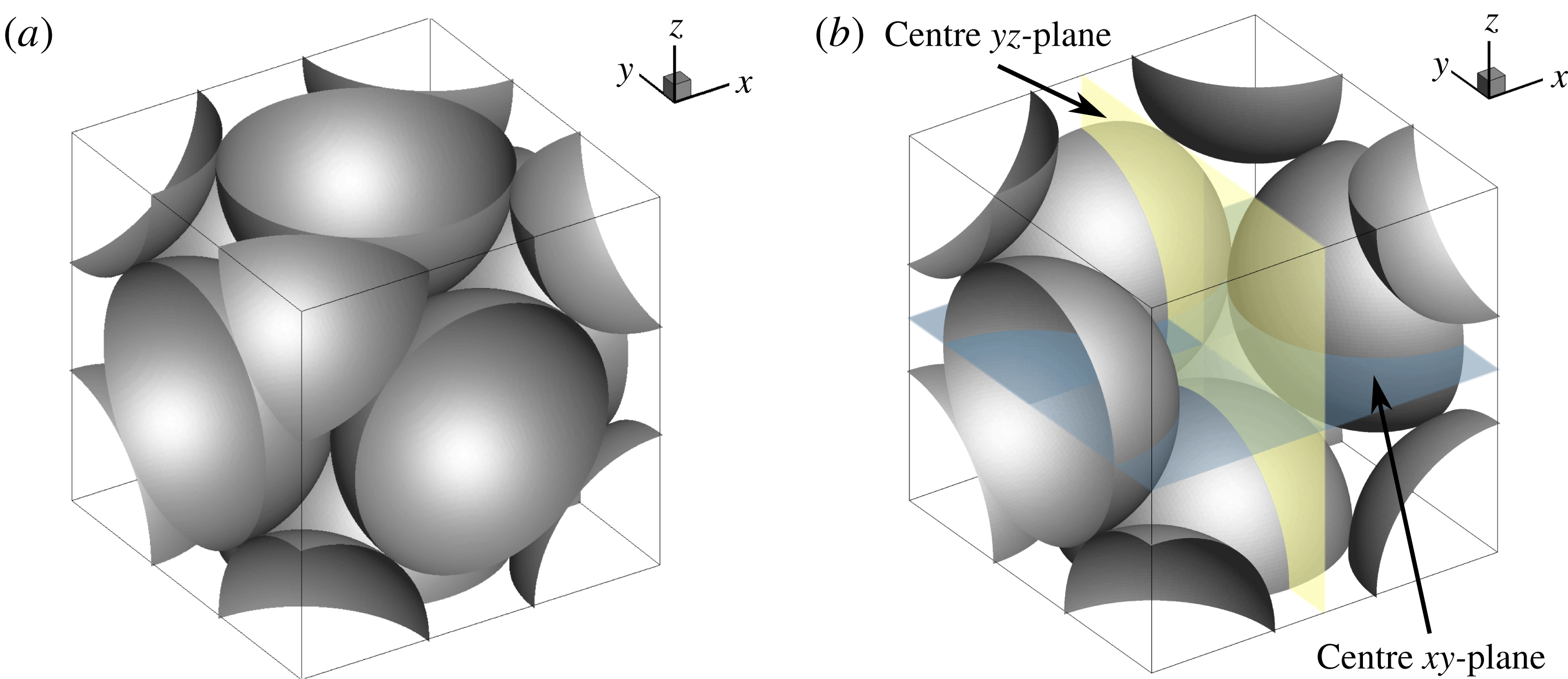
A porous face-centred cubic (FCC) unit cell (figure 1) is adopted for the present direct numerical simulations. The domain has half a sphere entering at each face of the cube; and a half of a quarter sphere at each corner, forming a geometrically triple-periodic cube. Spherical particles with uniform size are used in the present configuration. The FCC structured packing creates a highly tortuous pore space and the lowest possible porosity (
 $\unicode[STIX]{x1D719}=0.26$
). Due to such extreme compactness of the geometry, the flow through the unit cell experiences rapid expansion and contraction. To drive the flow, a pressure gradient is imposed in the
 $x$
-direction and a triply periodic boundary condition is applied. A majority of the flow enters the cubic cell through the upstream open corners, converges into the centre pore, and then leaves the unit cell along downstream corners.
(a) Schematic of a face-centred porous unit cubic cell, (b) same as (a) except some particles are removed so that the flow region inside of the cell can be observed, and two perpendicular cross-sections are illustrated where the data will be presented.

Hill & Koch (Reference Hill and Koch2002) studied inertial and unsteady flow in the same geometry up to
 $Re_{H}=300$
. The present study extends their work to higher Reynolds numbers,
 $Re_{H}=300$
, 500, and 1000, ranging from unsteady inertial to turbulent regimes. Note that the definition of Reynolds number used by Hill & Koch (Reference Hill and Koch2002) is different from the one used in the present work. In Hill & Koch (Reference Hill and Koch2002), the Reynolds number is defined as
 $$\begin{eqnarray}\displaystyle Re_{HK}=\frac{\overline{\langle u_{x}\rangle }(D_{B}/2)}{\unicode[STIX]{x1D708}_{\unicode[STIX]{x1D6FE}}}, & & \displaystyle\end{eqnarray}$$
where
 $\overline{\langle u_{x}\rangle }$
is the mean superficial velocity and is related to the mean intrinsic average velocity as
 $\overline{\langle u_{x}\rangle }=\overline{\langle u_{x}\rangle ^{\unicode[STIX]{x1D6FE}}}\unicode[STIX]{x1D719}$
. The Reynolds number adopted by Hill & Koch (Reference Hill and Koch2002) can be converted to the more commonly used definition and followed in the present work (
 $Re_{H}$
) through
 $$\begin{eqnarray}\displaystyle Re_{H}=Re_{HK}\frac{2}{1-\unicode[STIX]{x1D719}}. & & \displaystyle\end{eqnarray}$$
In the remainder of this work, the terms sphere or particle may be used interchangeably to indicate the solid phase. The numerical calculations are set up with dimensionless variables. Thus, the exact length scales of pores and particles are removed from the problem. However, we have assumed that the continuum Navier–Stokes equations are valid for these studies; thus, these results would not apply to systems with nanoscale solid particles, where the continuum assumption may cease to be valid.
Although a single unit cell is used in the present work, computations were performed in a
 $3\times 3\times 3$
configuration as well to evaluate effects of the periodic boundary condition on the flow structures. As is shown later, the integral scales for all Reynolds numbers studied in this work are much smaller than the particle diameter and thus the unit cell domain showed little variation in statistics compared to a larger domain.
2.2 Numerical approach
The numerical approach used in the current work is based on a fictitious domain method that can handle arbitrary shaped immersed objects without requiring body-fitted grids (Apte, Martin & Patankar Reference Apte, Martin and Patankar2009). Uniform Cartesian grids are used in the entire simulation domain, including both fluid and solid phases. An additional body force is imposed on the solid part to enforce the rigidity constraint and satisfy the no-slip boundary condition. The absence of highly skewed unstructured mesh at the sphere surface has been shown to accelerate the convergence and lower the uncertainty for porous media simulations (Finn & Apte Reference Finn and Apte2013). The following governing equations are solved over the entire domain, including the region within the solid phase. The rigidity constraint force,
 $\boldsymbol{f}$
, is applied that is non-zero only in the solid region.
 $$\begin{eqnarray}\displaystyle & \displaystyle \unicode[STIX]{x1D735}\boldsymbol{\cdot }\boldsymbol{u}=0 & \displaystyle\end{eqnarray}$$
 $$\begin{eqnarray}\displaystyle & \displaystyle \unicode[STIX]{x1D70C}_{\unicode[STIX]{x1D6FE}}\left[\frac{\unicode[STIX]{x2202}\boldsymbol{u}}{\unicode[STIX]{x2202}t}+(\boldsymbol{u}\boldsymbol{\cdot }\unicode[STIX]{x1D735})\boldsymbol{u}\right]=-\unicode[STIX]{x1D735}p+\unicode[STIX]{x1D707}_{\unicode[STIX]{x1D6FE}}\unicode[STIX]{x1D6FB}^{2}\boldsymbol{u}+\unicode[STIX]{x1D70C}_{\unicode[STIX]{x1D6FE}}\boldsymbol{g}+\boldsymbol{f}. & \displaystyle\end{eqnarray}$$
Here,
 $\boldsymbol{u}$
is the velocity vector with components given by
 $\boldsymbol{u}=(u_{x},u_{y},u_{z})$
,
 $\unicode[STIX]{x1D70C}_{\unicode[STIX]{x1D6FE}}$
is the fluid density,
 $\unicode[STIX]{x1D707}_{\unicode[STIX]{x1D6FE}}$
is the fluid dynamic viscosity,
 $p$
is the pressure and
 $\boldsymbol{g}$
is the gravitational acceleration. The details of the algorithm as well as verification and validation studies have been reported elsewhere (Apte et al.
Reference Apte, Martin and Patankar2009).
A fully parallel, structured, collocated grid solver is used in this work. This solver has been developed and thoroughly verified and validated for a range of test cases including flow over a cylinder and sphere for different Reynolds numbers, flow over touching spheres at different orientations, flow developed by an oscillating cylinder, among others (Finn & Apte Reference Finn and Apte2013). The solver has also been used to perform a direct one-to-one comparison with a body-fitted grid solver with known second-order accuracy for steady inertial, unsteady inertial and turbulent flow through porous media. The details of this comparison (Finn & Apte Reference Finn and Apte2013) focused on addressing issues such as the necessary grid resolution needed near the wall, the resolution of touching spheres and contact points, the quality of the solution as compared with the body-fitted solver, and validation by comparison with the experimental work of Suekane et al. (Reference Suekane, Yokouchi and Hirai2003). This latter effort allowed us to establish the grid resolution requirement (on a per particle diameter basis) required for predicting the unsteady flow-field in a packed porous beds to within a 5 % uncertainty (based on the grid convergence index (known as GCI) (Roache Reference Roache2003)). Turbulent flow at a Reynolds number of 600 was also computed in the same configuration and compared with the body-fitted approach; the results demonstrated a good match between the fictitious domain solver and the body-fitted approach. Finally, the flow solver was validated by comparing the numerical predictions with PIV data for flow through a randomly-oriented packed bed (Wood et al. Reference Wood, Apte, Liburdy, Ziazi, He, Finn and Patil2015) to show the good predictive capability of the numerical approach.
Following Hill & Koch (Reference Hill and Koch2002), a constant pressure gradient
 $\unicode[STIX]{x1D735}p$
, whose magnitude is proportional to the dimensionless body force
 $F$
, is specified to drive the flow
 $$\begin{eqnarray}\displaystyle |\unicode[STIX]{x1D735}p|=\frac{18\,\unicode[STIX]{x1D707}_{\unicode[STIX]{x1D6FE}}\,(1-\unicode[STIX]{x1D719})\,\overline{\langle u_{x}\rangle }}{D_{B}^{2}}F, & & \displaystyle\end{eqnarray}$$
where, (
 $1-\unicode[STIX]{x1D719}$
) is the solid volume fraction. The body force
 $F$
changes with Reynolds number according to the fit obtained by Hill & Koch (Reference Hill and Koch2002) and is given as
 $$\begin{eqnarray}\displaystyle & \displaystyle F=365+10.9\left(\frac{1-\unicode[STIX]{x1D719}}{2}Re_{H}\right)\quad (27<Re_{H}<216), & \displaystyle\end{eqnarray}$$
 $$\begin{eqnarray}\displaystyle & \displaystyle F=462+9.85\left(\frac{1-\unicode[STIX]{x1D719}}{2}Re_{H}\right)\quad (Re_{H}\geqslant 216). & \displaystyle\end{eqnarray}$$
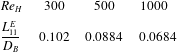
As shown in table 1, a posteriori calculation of body force in the flow direction, balancing the component of stress on the sphere surfaces for different Reynolds numbers, shows a good agreement with the above correlation.
Comparison of the body force obtained from correlation (2.7) and that obtained from the total stress on sphere surfaces required to maintain the same Reynolds numbers.

2.3 Grid resolution and convergence
Resolving all scales of turbulence in a densely packed porous medium requires a very fine resolution grid, especially near contact points present in the touching spherical particles. Estimating the a priori grid resolution is critical to assure sufficient resolution and yet not make a significant overestimation, so as to keep the size of the simulation tractable. Recently, Chu et al. (Reference Chu, Weigand and Vaikuntanathan2018) conducted direct numerical simulations of turbulent flows in a high porosity porous bed of regularly-packed squared cylinders. Their configuration had non-touching cylinders with grid resolution of about 94–100 grid points per unit square length for Reynolds numbers up to 1500. In the present work, a thorough analysis of the grid resolution requirement and related convergence study were conducted to ensure that the results obtained are not influenced by grid resolution.
Using an overall momentum balance, the pressure drop (in the mean flow direction) per unit length,
 $\unicode[STIX]{x0394}p/L$
, through an arranged pack of spheres with porosity
 $\unicode[STIX]{x1D719}$
and specific surface
 $D_{B}/6$
is balanced by the component in the flow direction of the area-averaged total stress on the solid wall, computed as
 $$\begin{eqnarray}\displaystyle \langle \unicode[STIX]{x1D70E}_{w,x}\rangle _{A}=\frac{1}{A_{\unicode[STIX]{x1D705}\unicode[STIX]{x1D6FE}}}\int \unicode[STIX]{x1D70E}_{w,x}\,\text{d}\,A_{\unicode[STIX]{x1D705}\unicode[STIX]{x1D6FE}}, & & \displaystyle\end{eqnarray}$$
where
 $\unicode[STIX]{x1D70E}_{w,x}$
is the component of the total stress on the wall, including the wall shear and turbulent stresses, in the main flow direction,
 $A_{\unicode[STIX]{x1D705}\unicode[STIX]{x1D6FE}}$
is the area of the interface between fluid and solid phases,
 $\unicode[STIX]{x1D705}$
represents the solid phase, and
 $\langle \,\cdot \,\rangle _{A}$
is the area-averaging operator. A balance of the pressure and stress forces leads to
 $$\begin{eqnarray}\displaystyle \langle \unicode[STIX]{x1D70E}_{w,x}\rangle _{A}=\frac{\unicode[STIX]{x0394}p}{L}\frac{D_{B}}{6}\left(\frac{\unicode[STIX]{x1D719}}{1-\unicode[STIX]{x1D719}}\right). & & \displaystyle\end{eqnarray}$$
The above equation can be rewritten in terms of the modified friction factor,
 $f$
(Dybbs & Edwards Reference Dybbs, Edwards, Bear and Corapcioglu1984), to obtain
 $$\begin{eqnarray}\displaystyle \langle \unicode[STIX]{x1D70E}_{w,x}\rangle _{A}=f\frac{\unicode[STIX]{x1D70C}(\overline{\langle u_{x}\rangle ^{\unicode[STIX]{x1D6FE}}})^{2}}{6},\quad \text{where }f=\frac{\unicode[STIX]{x0394}p}{L}\frac{D_{B}}{\unicode[STIX]{x1D70C}(\overline{\langle u_{x}\rangle ^{\unicode[STIX]{x1D6FE}}})^{2}}\frac{\unicode[STIX]{x1D719}}{1-\unicode[STIX]{x1D719}}. & & \displaystyle\end{eqnarray}$$
For fully resolved DNS in wall bounded flows, the first grid point in the wall coordinate should be located at less than or equal to
 $\unicode[STIX]{x1D6FF}^{+}=\unicode[STIX]{x1D6FF}u_{\unicode[STIX]{x1D70F}}/\unicode[STIX]{x1D708}_{\unicode[STIX]{x1D6FE}}\sim 1$
, where
 $u_{\unicode[STIX]{x1D70F}}=\sqrt{\langle \unicode[STIX]{x1D70F}_{w,x}\rangle _{A}/\unicode[STIX]{x1D70C}}$
is the friction velocity,
 $\langle \unicode[STIX]{x1D70F}_{w,x}\rangle _{A}$
is the area-averaged wall shear stress and is defined in a similar way to (2.8), and
 $\unicode[STIX]{x1D6FF}$
is the dimensional distance normal to the solid surface. The area-averaged wall shear stress can be assumed to be some fraction (
 $\unicode[STIX]{x1D6FD}$
) of the total stress, such that,
 $$\begin{eqnarray}\displaystyle \unicode[STIX]{x1D6FD}=\langle \unicode[STIX]{x1D70F}_{w,x}\rangle _{A}/\langle \unicode[STIX]{x1D70E}_{w,x}\rangle _{A}. & & \displaystyle\end{eqnarray}$$
Using (2.10) and (2.11) and definition of
 $\unicode[STIX]{x1D6FF}^{+}$
, the normalized grid spacing can be written in terms of the Reynolds number, porosity, and the friction factor as
 $$\begin{eqnarray}\displaystyle \frac{D_{B}}{\unicode[STIX]{x1D6FF}}=\frac{1}{\unicode[STIX]{x1D6FF}^{+}}\sqrt{\frac{\unicode[STIX]{x1D6FD}f}{6}}\frac{1-\unicode[STIX]{x1D719}}{\unicode[STIX]{x1D719}}Re_{H}. & & \displaystyle\end{eqnarray}$$
Gunjal, Ranade & Chaudhari (Reference Gunjal, Ranade and Chaudhari2005) conducted RANS simulations in face-centred cubic arrangements of packed spheres to show that the ratio,
 $\unicode[STIX]{x1D6FD}$
, of the averaged surface drag to total drag was of the order of
 $0.21$
for
 $Re_{H}$
up to
 $1000$
. Using
 $\unicode[STIX]{x1D6FD}=0.25$
and taking
 $\unicode[STIX]{x1D6FF}^{+}=1$
yields an estimate of
 $D_{B}/\unicode[STIX]{x1D6FF}\sim 800$
for
 $Re_{H}=1000$
. However, an actual grid refinement was performed to obtain grid converged mean and root-mean-square (r.m.s.) velocities in the porous geometry as discussed below. This study showed that the requirement of
 $\unicode[STIX]{x1D6FF}^{+}=1$
is too stringent for the present configuration involving flow separations and could be relaxed to
 $\unicode[STIX]{x1D6FF}^{+}=3$
(yielding
 $D_{B}/\unicode[STIX]{x1D6FF}\sim 267$
) to obtain fully converged predictions.
To obtain a more accurate estimate for the required grid resolution requirements, three-dimensional (3-D) DNS studies were performed at
 $Re_{H}=500$
and
 $1000$
in a unit cell of FCC spheres with a systematic grid refinement study. Successive refinements using
 $48$
,
 $64$
,
 $96$
,
 $112$
,
 $128$
and
 $144$
grid points per particle diameter
 $D_{B}$
were examined. A grid-converged solution was obtained for first-order (mean flow) as well as second-order statistics (TKE) for
 $Re_{H}=500$
at the resolution of
 $D_{B}/\unicode[STIX]{x1D6FF}=96$
. For
 $Re_{H}=1000$
, the mean flow converged at
 $D_{B}/\unicode[STIX]{x1D6FF}=144$
, whereas, TKE continued to show small changes even at the highest resolution. In order to obtain a high-fidelity DNS data set and provide sufficient resolution in the sphere contact regions, a refined grid based on
 $D_{B}/\unicode[STIX]{x1D6FF}=250$
was used to resolve the pore-scale flow structures, which results in
 $353^{3}$
(approximately 44 million) degrees of freedom for each case. Finn (Reference Finn2013) conducted a grid convergence study on the same geometry and also concluded that a grid based on
 $D_{B}/\unicode[STIX]{x1D6FF}=250$
provides an accurate representation of the flow field. In wall units,
 $\unicode[STIX]{x1D6FF}^{+}$
is estimated to be less than 1 for
 $Re_{H}=300$
, close to 1 for
 $Re_{H}=500$
and about 3 for
 $Re_{H}=1000$
. This grid resolution is still much finer than the finest one used by Chu et al. (Reference Chu, Weigand and Vaikuntanathan2018) (who used
 ${\sim}94$
grids per unit length) and is thus able to resolve the flow field in a densely packed porous bed accurately.
The direct numerical simulations with such fine grid resolution were conducted using the Stampede2 supercomputer at the Texas Advanced Computing Center of The University of Texas at Austin. The total TKE was monitored over time; initially the TKE is large, and then it decreases (approximately) to a constant value after an initial transient period. This was used as a criterion to confirm that a stationary state has been reached. It took about
 $130T_{f}$
(where
 $T_{f}=L/\overline{\langle u_{x}\rangle ^{\unicode[STIX]{x1D6FE}}}$
is the flow through time and
 $L$
is the length of the unit cube) for
 $Re_{H}=300$
and about
 $80T_{f}$
for
 $Re_{H}=1000$
to reach a stationary state. After a stationary state was achieved, the computations were continued for an additional
 $80T_{f}$
for each Reynolds number to collect flow statistics. This time period was found to be large enough to obtain fully converged statistics.
3 Results
In this section, detailed flow analyses are presented as follows:
(i) The mean flow contours are shown to qualitatively describe the flow. The turbulence kinetic energy and its budget are presented next to identify the peak production locations, unique features such as regions of negative total TKE production and the role of pressure, turbulent and viscous transport.
(ii) Scales of turbulence obtained from auto-correlation and energy spectra are computed to determine if turbulence structures of the order or larger than the pore or particle size are present in this low porosity configuration. In addition, the correlations are used to obtain energy spectra and Lagrangian time scales using a simple scaling model to see if the model would be applicable for a representative volume of computation.
(iii) Probability density functions of the components of velocity and vorticity are investigated and contrasted with Gaussian distribution for different
 $Re_{H}$
. Statistics of relative helicity are also studied to quantify the degree to which velocity and vorticity are aligned at different Reynolds numbers. In addition, their behaviour at these higher Reynolds numbers is compared with simulations at lower
 $Re_{H}$
by Hill & Koch (Reference Hill and Koch2002) to identify the effects of geometric confinement over a wider range of
 $Re_{H}$
.
(iv) Finally, a detailed analysis of the velocity gradient tensor is performed to visualize the vortical structures, anisotropy distribution and how the turbulence structures are altered in a highly tortuous and complex configuration. Specifically, the turbulence structure in regions of peak production is explored in detail. Categorizing the pore space into different regions corresponding to the turbulence structures observed (two-dimensional (2-D), cigar shaped, isotropic, among others), allows quantifying the complex nature of the turbulence in porous media.
3.1 Mean flow and turbulence statistics
In order to get a good understanding of the simulated flow topology, distributions of the mean velocity magnitude
 $\overline{U}_{m}$
and the turbulent kinetic energy are presented first. Two centre slices (see figure 1
b) are chosen as representative sections for visualizations. One is the centre
 $xy$
-plane, where the mean flow is going from the left-hand side to the right-hand side; the other the centre
 $yz$
-plane, where the mean flow in going into the slice. In addition, the TKE budget and variation of the production/dissipation of TKE within the confined porous geometry are analysed.
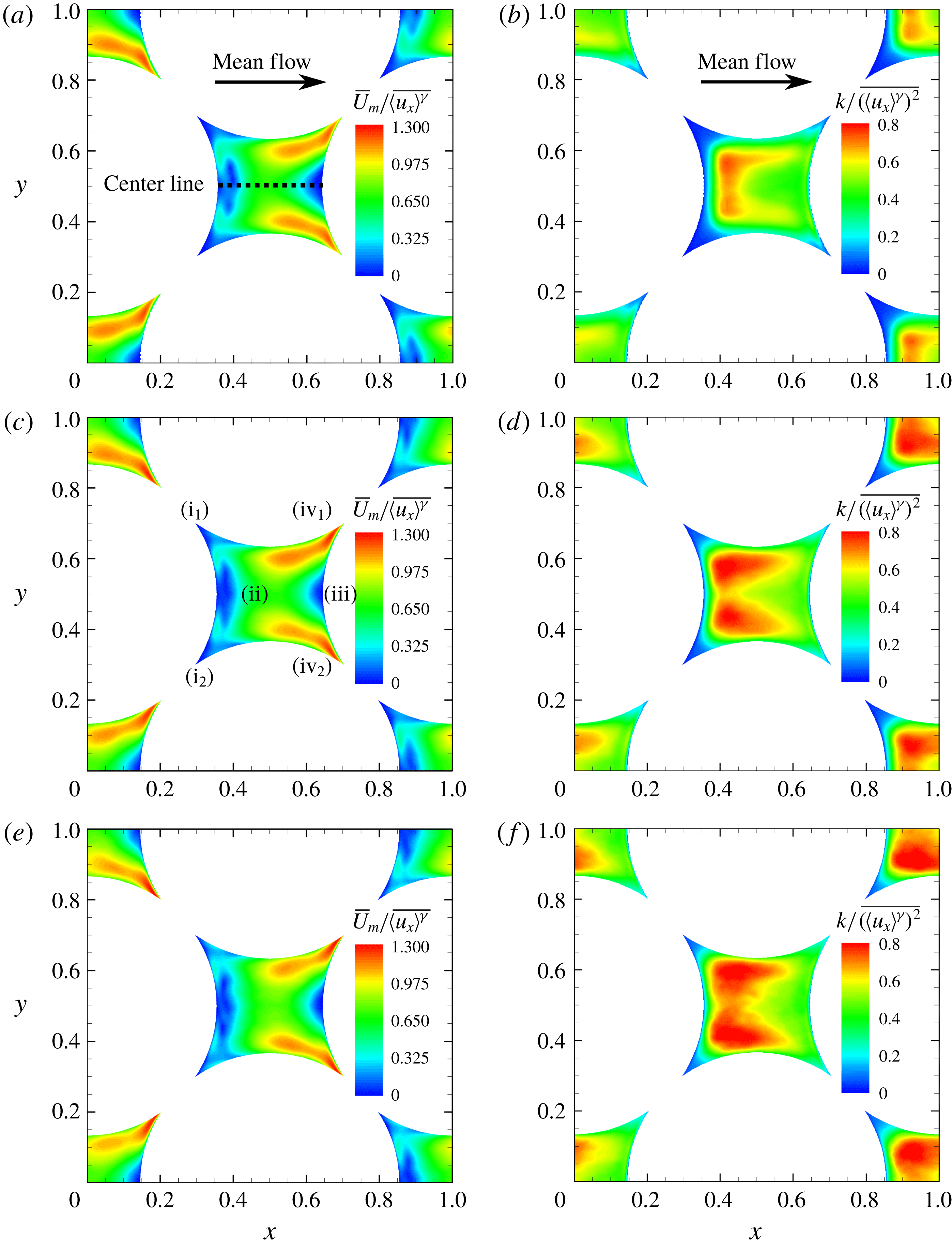
The left column shows the contours of the mean velocity magnitude (
 $\overline{U}_{m}$
) normalized by the interstitial velocity on the centre
 $xy$
-plane; and the right-hand side TKE normalized by the square of interstitial velocity. The figures at the first row (a,b) are for
 $Re_{H}=300$
, second (c,d)
 $Re_{H}=500$
and third (e,f)
 $Re_{H}=1000$
.

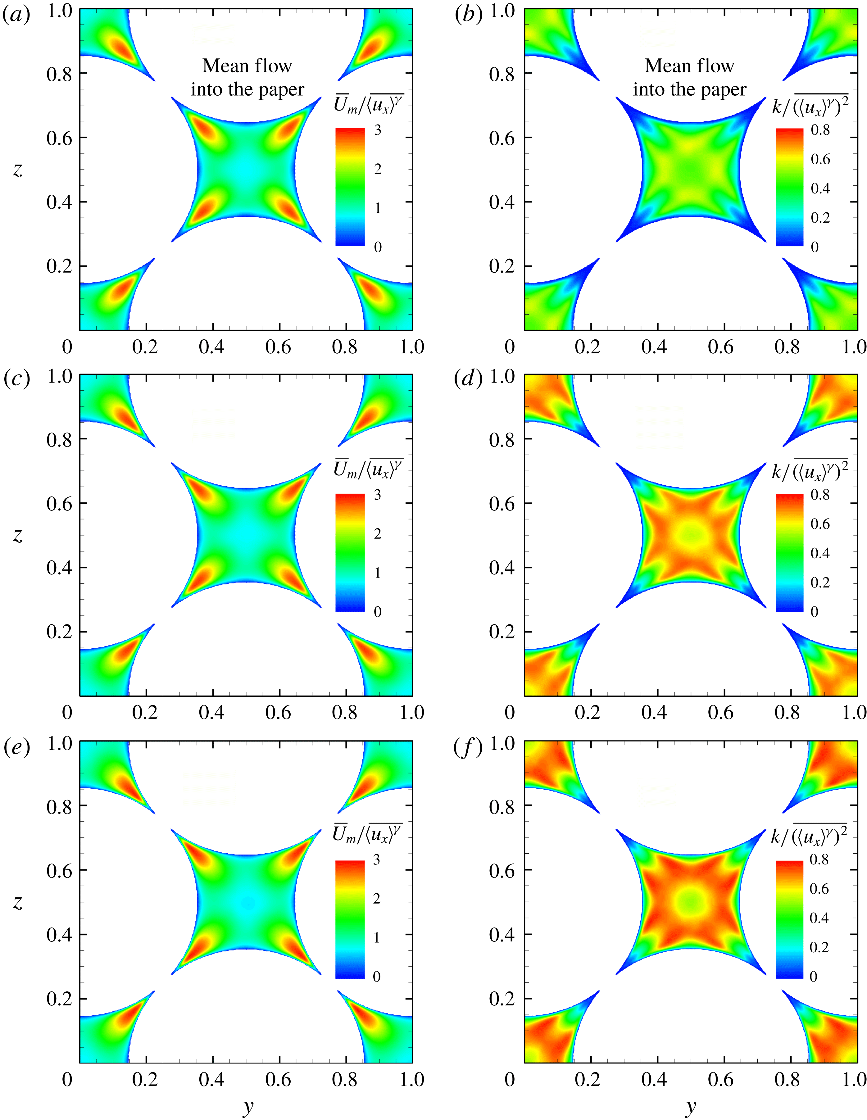
The left column shows the contours of the mean velocity magnitude (
 $\overline{U}_{m}$
) normalized by the interstitial velocity on the centre
 $yz$
-plane; and the right-hand side the TKE normalized by the square of interstitial velocity. The figures at the first row (a,b) are for
 $Re_{H}=300$
, second (c,d)
 $Re_{H}=500$
and third (e,f)
 $Re_{H}=1000$
.

3.1.1 Mean velocity magnitude distribution
The compactness and confinement of the geometry creates strong acceleration and deceleration of the flow within the pore space. To visualize the flow field, contours of the normalized temporal mean velocity magnitude (
 $\overline{U}_{m}$
) in the centre
 $xy$
-plane are plotted in figures 2(a), 2(c), and 2(e) for each Reynolds number, where
 $\overline{U}_{m}$
is calculated as
 $\sqrt{\overline{u_{x}}^{2}+\overline{u_{y}}^{2}+\overline{u_{z}}^{2}}$
and normalized by the mean interstitial velocity
 $\overline{\langle u_{x}\rangle ^{\unicode[STIX]{x1D6FE}}}$
. An almost identical distribution of the normalized fields for
 $\overline{U}_{m}$
is observed regardless of the Reynolds number. The mean flow enters the centre pore from the left-hand side corners (regions labelled by (
 $\text{i}_{1}$
) and (
 $\text{i}_{2}$
) in figure 2
c) and accelerates to region (ii) due to the geometric constrictions; then the mean flow at the centre starts to decelerate as it encounters the particle at region (iii), similar to an impinging jet. The flow then accelerates in the spanwise directions and leaves the pore through the right-hand side corners (regions (
 $\text{iv}_{1}$
) and (
 $\text{iv}_{2}$
)). The acceleration and deceleration close to the right-hand side sphere can be seen as transfer of momentum from the streamwise to the spanwise directions due to the bounding of the solid phase. The pattern of mean velocity distribution indicates how the mean flow in the pore is affected by the geometry. High Reynolds number flow features, such as wake and large scale vortex shedding in an external flow behind a spherical particle, are not observed in this low porosity bed. A weak wake-like structure (small negative mean velocity just behind the left-hand side sphere near region (ii) in figure 2
c) is present, but is confined to a small region. The closely packed particles in the low porosity FCC configuration tend to break down large scale flow structures and prevent the generation of a significant wake region. This is in contrast to the high porosity studies of square cylindrical porous structures conducted by Chu et al. (Reference Chu, Weigand and Vaikuntanathan2018), where distinct wakes and flow separation were identified.
Figures 3(a), 3(c), and 3(e) show the distributions of the mean velocity magnitude on the centre
 $yz$
-plane. On this slice, the mean flow is moving perpendicularly into the page and there is a distinguished region with high velocity magnitude near each corner of the centre pore. Similar to what is observed from figures 2(a), 2(c) and 2(e), the mean velocity field does not change significantly at different flow rates.
3.1.2 TKE distribution
The TKE distribution presents a strong dependency on the Reynolds number, which is different from the uniform distribution of the mean velocity field described in the previous section. The turbulent kinetic energy
 $k$
, defined as
 $(1/2)(\overline{{u_{x}^{\prime }}^{2}}+\overline{{u_{y}^{\prime }}^{2}}+\overline{{u_{z}^{\prime }}^{2}})$
, is normalized by the square of the mean interstitial velocity
 $(\overline{\langle u_{x}\rangle ^{\unicode[STIX]{x1D6FE}}})^{2}$
. Here the temporal fluctuation velocity
 $u_{x}^{\prime }$
is defined as
 $u_{x}-\overline{u_{x}}$
. Figures 2(b), 2(d) and 2(f) illustrate the distribution of normalized TKE on the centre
 $xy$
-plane. Substantial disparities in the TKE distribution can be observed at different Reynolds numbers. Firstly, the overall magnitude of the TKE increases with
 $Re_{H}$
. Secondly, with increasing flow rate, the TKE values in the centre region of the pore remain substantially high. It also suggests that the flow through the pore, although bounded by curved particle walls, is different from simple channel/duct flows even with complex boundaries (Orlandi, Modesti & Pirozzoli Reference Orlandi, Modesti and Pirozzoli2018) wherein the TKE reaches a peak value near the boundaries and then decreases in the centre region.
The normalized TKE distributions on the centre
 $yz$
-plane shown in figures 3(b), 3(d) and 3(f) indicate similar trends: the magnitude of the TKE increased with increasing
 $Re_{H}$
; the distribution pattern changes noticeably as well. In this slice, some similarities with duct flows are noticed. Away from the wall, the TKE increases and reaches a peak value; and then decreases as we approach the core region of the pore. The homogeneous particle packing involving four particles aligned together seem to form a locally duct-like flow pattern in this section. However, it disappears in other sections away from the centre
 $yz$
-plane, owing to the three-dimensional nature of the spherical particles.
3.1.3 TKE budget
To better understand the mechanism of TKE transport at the pore-scale, the TKE budget including production, dissipation and all the transport terms in the TKE transport equation (equation (3.1), where
 $k$
is the turbulent kinetic energy) are explicitly computed. The balance between the gain and loss of kinetic energy in the budget has been computed locally as well as globally for the entire flowfield. The average error of the TKE budgets are within
 $5\,\%$
for all three cases. The transport equation for turbulent kinetic energy is given by
 $$\begin{eqnarray}\displaystyle \underbrace{\frac{\unicode[STIX]{x2202}k}{\unicode[STIX]{x2202}t}}_{\mathit{Unsteady\,term}}+\underbrace{\overline{u_{j}}\frac{\unicode[STIX]{x2202}k}{\unicode[STIX]{x2202}x_{j}}}_{\mathit{Mean\,advection}} & = & \displaystyle \underbrace{-\overline{u_{i}^{\prime }u_{j}^{\prime }}\frac{\unicode[STIX]{x2202}\overline{u_{i}}}{\unicode[STIX]{x2202}x_{j}}}_{\mathit{Production}\,(P)}-\underbrace{\unicode[STIX]{x1D708}_{\unicode[STIX]{x1D6FE}}\overline{\frac{\unicode[STIX]{x2202}u_{i}^{\prime }}{\unicode[STIX]{x2202}x_{j}}\frac{\unicode[STIX]{x2202}u_{i}^{\prime }}{\unicode[STIX]{x2202}x_{j}}}}_{\mathit{Dissipation}\,(\unicode[STIX]{x1D716})}\nonumber\\ \displaystyle & & \displaystyle +\,\frac{\unicode[STIX]{x2202}}{\unicode[STIX]{x2202}x_{j}}\left[\underbrace{\unicode[STIX]{x1D708}_{\unicode[STIX]{x1D6FE}}\frac{\unicode[STIX]{x2202}k}{\unicode[STIX]{x2202}x_{j}}}_{\mathit{Viscous\,transport}}-\underbrace{\overline{\frac{1}{2}u_{i}^{\prime }u_{i}^{\prime }u_{j}^{\prime }}}_{\mathit{Turbulent\,transport}}-\underbrace{\frac{1}{\unicode[STIX]{x1D70C}_{\unicode[STIX]{x1D6FE}}}\overline{p^{\prime }u_{j}^{\prime }}}_{\mathit{Pressure\,transport}}\right],\quad\end{eqnarray}$$
where
 $P$
represents the production and
 $\unicode[STIX]{x1D716}$
the dissipation rate of TKE, respectively. TKE production normally serves as the source term in the TKE transport equation. The production term arising from the Reynolds stress working on the background mean shear extracts energy from the mean flow field and is typically expected to be positive. The dissipation term represents the transfer of the kinetic energy to heat under the effect of viscosity. Thus, it acts as a sink term in the TKE transport equation. If production and dissipation are in balance, the turbulence is in an equilibrium state.
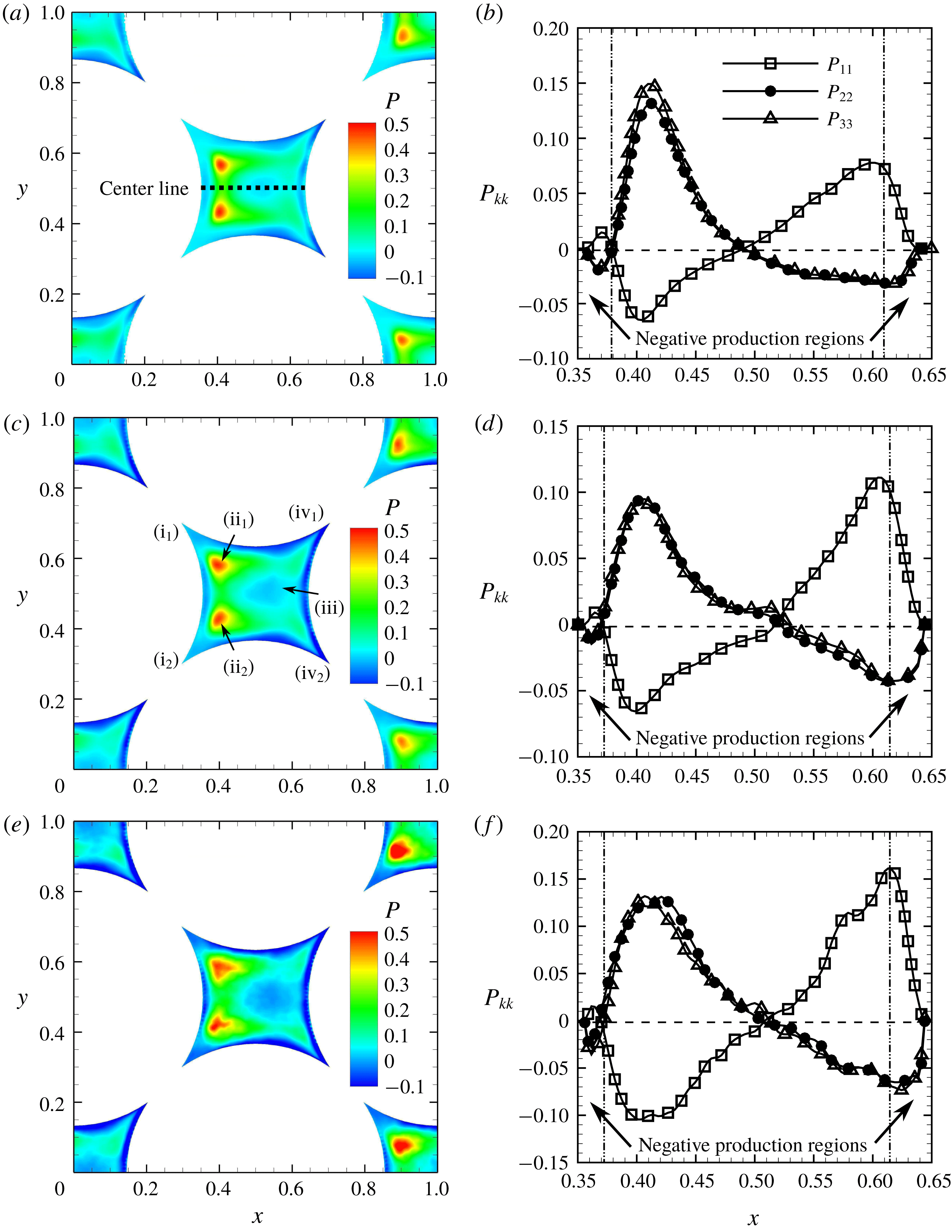
Distribution of the normalized net production of TKE (
 $P$
) and its normal components (
 $P_{kk}$
): the left column shows contours of normalized TKE production on the centre
 $xy$
-plane; and the right column shows variation of the three normal components of the production along the centre line. (a,b)
 $Re_{H}=300$
; (c,d)
 $Re_{H}=500$
; (e,f)
 $Re_{H}=1000$
.

Figures 4(a), 4(c) and 4(e) show the distribution of the net normalized TKE production (
 $P$
) in the centre
 $xy$
-plane for the three Reynolds numbers of 300, 500 and 1000, respectively. For the centre pore, the peak TKE production occurs just behind the left particle on either side of the centre line (regions
 $\text{ii}_{1}$
and
 $\text{ii}_{2}$
in figure 4
c). The size of the peak production region also increases with increasing Reynolds number. More importantly, it is clear from the contour plots that negative values of net production are observed near the surfaces of the particles (regions iii,
 $\text{iv}_{1}$
and
 $\text{iv}_{2}$
) especially near the flow exit regions. In most turbulent flows, the net TKE production term mainly remains positive, indicating that the energy is extracted from mean flow and fed into turbulence. However, this term being negative for the present cases, implies the unusual condition that the energy transport process is reversed. Turbulence is providing energy to maintain the mean flowfield. It is rare to observe such phenomenon and is attributed to the complex nature of the tortuous flow paths created by the porous geometry.
To further understand such phenomenon, the axial variation of the normal components of production,
 $P_{11}$
,
 $P_{22}$
and
 $P_{33}$
, are plotted along the centre line for the three different Reynolds numbers in figures 4(b), 4(d) and 4(f), respectively. The normal components of production,
 $P_{kk}$
, computed as
 $-\overline{({u_{k}}^{\prime })^{2}}(\unicode[STIX]{x2202}\overline{u_{k}}/\unicode[STIX]{x2202}x_{k})$
, are dominant along the centre line. At the edge of the left sphere (
 $x=0.35$
), all components of production are zero. As we move away from the left sphere surface, the axial component
 $P_{11}$
is positive, whereas the spanwise components,
 $P_{22}$
and
 $P_{33}$
, are negative. Although individual components of TKE production can be either positive or negative, the net summation of these components turns out to be negative in this small wake region directly behind the left sphere. Moving further to the right, the axial component turns to be negative and the other two components become positive, all peaking at about
 $x=0.42$
, reaching almost zero values at the midway point
 $x=0.5$
, and then switch signs with a peak at about
 $x=0.61$
. The net production of TKE is positive in this centre region,
 $0.38\leqslant x\leqslant 0.61$
. Approaching the stagnation point near the right sphere,
 $P_{11}$
is positive but
 $P_{22}$
and
 $P_{33}$
are negative, such that the net production becomes negative. It is also noteworthy that,
 $P_{22}$
and
 $P_{33}$
are mostly identical owing to the symmetry in the flow geometry.
In the negative production regions, the spanwise components,
 $P_{22}$
and
 $P_{33}$
are negative with the streamwise component
 $P_{11}$
being positive. In order to reveal the underlying physics related to this phenomenon, the production term is decomposed for more detailed examination. Here
 $P_{ij}$
is defined as the negative product of Reynolds stress
 $\overline{u_{i}^{\prime }u_{j}^{\prime }}$
multiplied by the mean strain rate
 $\unicode[STIX]{x2202}\overline{u_{i}}/\unicode[STIX]{x2202}x_{j}$
, where the normal components of Reynolds stress
 $\overline{{u_{i}}^{^{\prime }2}}$
are always positive. So the positivity of the normal TKE production components is exclusively determined by the mean rate of strain, i.e. whether the mean flow is accelerating or decelerating.
The net production near the exit (regions
 $\text{iv}_{1}$
and
 $\text{iv}_{2}$
in figure 4
d) is discussed first. As shown in figure 2(c), the mean flow moves in the axial direction through the centre region of the pore and is decelerated by the particle surface on the right (region iii) similar to an impinging jet, then merges with the rest and exits the pore through the crevices. During this process, the flow is accelerating in spanwise directions, and decelerating in streamwise direction. As a result, the mean strain rates in
 $y$
- and
 $z$
-directions are positive, while negative in
 $x$
-direction. Together with the positive normal Reynolds stresses, the sum of negative production in the spanwise directions outnumbers that in the streamwise direction, which causes the net production to be negative near the stagnation point. A similar observation was reported by Nishino et al. (Reference Nishino, Samada, Kasuya and Torii1996) who observed negative production in the stagnation zone of an impinging jet.
In the entrance region (regions
 $\text{i}_{1}$
and
 $\text{i}_{2}$
in figure 4
d), the mechanism is similar except that there is no jet impingement. The flow goes into the pore through the corners on the left side of the unit cell and merges as it approaches the centre of the pore. Thus, the flow is accelerating in the spanwise directions and a confined wake near the left sphere is created by the merging flow, which leads to the negative mean strain rate in
 $x$
-direction; this results in a negative net production of TKE.
In summary, the mean flow acceleration and deceleration together with normal components of Reynolds stress are mainly responsible for the negative net production. Since the normal components of Reynolds stress are positive by definition, the locations of the acceleration and deceleration of mean flow actually determines where the negative production may happen. Observing from figures 2(a), 2(c) and 2(e), the mean flow field changes little with respect to Reynolds number. Consequently, regions with
 $-P$
are expected to locate at the same positions in the flowfield regardless of Reynolds number.
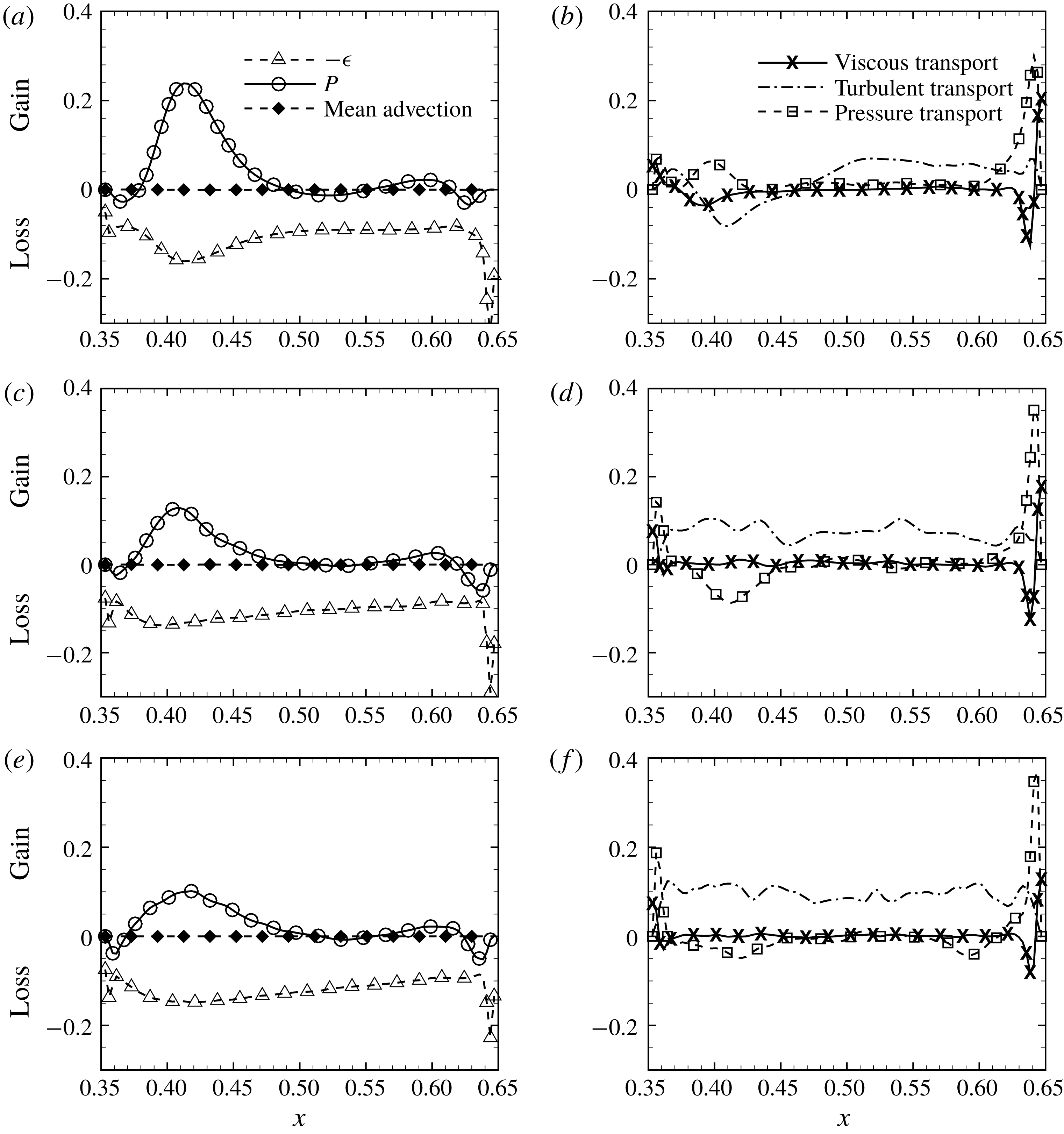
Figure 5 shows all the terms in the TKE transport equation along the centre line for the three values of
 $Re_{H}$
, respectively. Each term of the TKE budget, normalized by
 $(\overline{\langle u_{x}\rangle ^{\unicode[STIX]{x1D6FE}}})^{3}/D_{B}$
, is plotted, except the local unsteady term, which is essentially zero for stationary flows. As explained before, close to the surfaces of the left and right spheres, the net production term (
 $P$
) becomes negative giving rise to negative production. The dissipation term (
 $-\unicode[STIX]{x1D716}$
) peaks near the particle surfaces and is negative over the entire pore along the centre line. Moreover, production is not equal to the dissipation over most of the flow domain. Thus, the majority of the turbulent flow within the pore is not at an equilibrium state. The viscous transport is mostly zero in the centre region of the pore, but increases near the particle surfaces as expected. Although the fluctuation velocity
 $u_{i}^{\prime }$
is zero at the wall, the fluctuating strain rate
 $\unicode[STIX]{x2202}u_{i}^{\prime }/\unicode[STIX]{x2202}x_{j}$
is not, resulting in the non-zero viscous transport terms.
It is also interesting to note that the contribution from the turbulent transport term to the TKE budget is significant over the entire pore. Consequently, the triple correlation, which can be taken as the fluctuation velocity components working with the Reynolds stress, is redistributing the TKE over the entire flow regime. This is different from that of a channel or a duct flow wherein the contribution of the turbulent transport term is not significant (e.g. Pope Reference Pope2000). Such observations may be attributed to high turbulence intensities over the entire pore region as opposed to the wall-bounded regions of a duct flow, where the turbulent transport term is significant only near the wall.
In the negative production regions, the pressure transport term shows dominant and positive peaks for all Reynolds numbers. It is evident that the pressure plays an important role for the redistribution of TKE near the wall. The pressure transport term moves TKE close to the wall, especially to the wall on the right-hand (downstream) side of the pore. For
 $Re_{H}=500$
and
 $1000$
, the turbulent transport remains positive, and the pressure transport terms show a negative peak. For
 $Re_{H}=300$
, however, near the region where the net production shows a positive peak, the turbulent transport is found to be negative whereas the pressure transport is positive. This may be attributed to the fact that the flow at
 $Re_{H}=300$
is not fully developed into a turbulent flow. The smaller magnitude fluctuations in the velocity and pressure fields are likely to be causing these differences.
The TKE budgets along the centre line at
 $xy$
-plane: the left column shows the production, negative dissipation and mean advection terms; the right column the viscous transport, turbulent transport and pressure transport terms. (a) and (b) are for
 $Re_{H}=300$
, (c) and (d)
 $Re_{H}=500$
and (e) and (f)
 $Re_{H}=1000$
.

3.2 Turbulence scales and energy spectra
In order to study how turbulence scales change with Reynolds number in the complex geometry of the porous media, the turbulence intensity components in streamwise and spanwise directions are estimated for each Reynolds number. The
 $x$
-component r.m.s. velocity,
 $u_{x-rms}^{\prime }$
is computed by
 $$\begin{eqnarray}\displaystyle u_{x-rms}^{\prime }=\sqrt{\overline{u_{x}^{2}}-{\overline{u}_{x}}^{2}}, & & \displaystyle\end{eqnarray}$$
likewise for
 $u_{y-rms}^{\prime }$
and
 $u_{z-rms}^{\prime }$
.
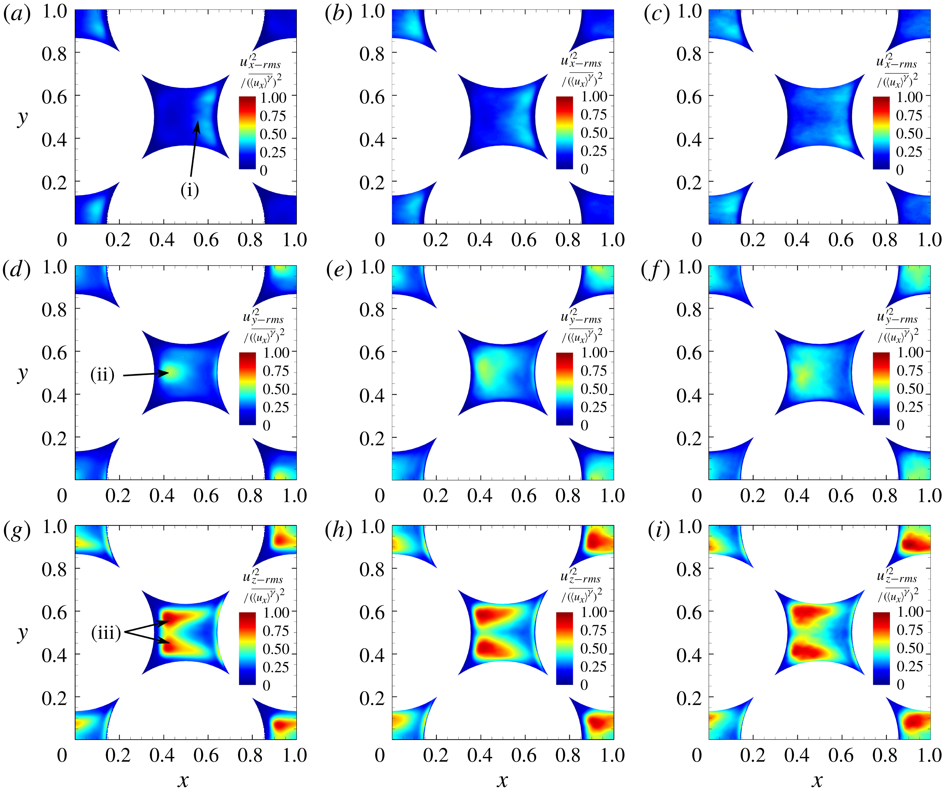
Contours for three components of turbulence intensity normalized by the square of interstitial velocity on the centre
 $xy$
-plane. Top row (a–c)
 $x$
-component of turbulence intensity, middle row (d–f)
 $y$
-component, and bottom row (g–i)
 $z$
-component; the figures in the first column (a,d,g) are for
 $Re_{H}=300$
, the second (b,e,h)
 $Re_{H}=500$
and the third column (c,f,i) for
 $Re_{H}=1000$
. Mean flow is from left to right.

Contours for the three components of turbulence intensity in the centre
 $xy$
-plane are shown in figure 6, showing significant differences in magnitude and distribution at each flow rate. The
 $x$
-component turbulence intensity is only heavily pronounced in the region close to the right-hand side particle (region (i) in figure 6
a), which is mostly attributed to the impingement-like flow in this region. Also, the high
 $x$
-component turbulence intensity region expands to the centre of the pore at higher Reynolds numbers (see figures 6
a–c), due to stronger inertial effects. In this centre
 $xy$
-plane, the
 $x$
-component of turbulence intensity, corresponding to the main flow direction, is weaker compared to the other two components regardless of
 $Re_{H}$
. The maximum value of
 $x$
-component turbulence intensity is about 80 % and 50 % of that for
 $y$
- and
 $z$
-components, respectively. Such an observation is qualitatively consistent with the results reported by Patil & Liburdy (Reference Patil and Liburdy2013).
The
 $y$
- and
 $z$
-components of turbulence intensity are discussed together in the following, because they are both spanwise components in homogeneous directions. On the centre
 $xy$
-plane, these two components are distributed in various patterns. The
 $y$
-component mostly concentrates near the left-hand side particle (region (ii) in figure 6
d). With increasing
 $Re_{H}$
, the regime with high
 $y$
-component turbulence intensity extends not only in the streamwise direction to the right-hand side of the centre pore, but also in the spanwise direction to both top and bottom particles (see figures 6
d–f). However for the
 $z$
-component, the distribution is substantially different. There are two distinct regions with high magnitude of
 $z$
-component turbulence intensity (regions (iii) in figure 6
g) near the left-hand side particle. In addition, the range of these high turbulence intensity regions grows with increasing
 $Re_{H}$
as shown in figure 6(g–i). More importantly, the shape of such regions is almost identical to the high TKE regions illustrated in figures 2(b), 2(d) and 2(f), indicating that the
 $z$
-component turbulence intensity has the most important contribution to total TKE at this particular plane. Although not shown here, it is noteworthy that, the distributions of
 $y$
- and
 $z$
-components of turbulence intensity on the centre
 $xy$
-plane are interchanged on the centre
 $xz$
-plane, due to the homogeneous and symmetric geometry of the FCC packing; and the
 $x$
-component distribution remains the same.
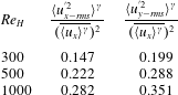
To investigate the overall characteristics of both the streamwise and spanwise components of turbulence intensity, and for purposes of comparison, we have computed the intrinsic spatial average of these r.m.s. velocities (normalized by the square of intrinsic averaged velocity) as shown in table 2. Because of the periodicity and symmetry in the computational domain, the volume-averaged r.m.s. velocity in the
 $z$
-direction is similar to that in the
 $y$
-direction and hence not included here.
Table 2 shows that the turbulence intensity in both streamwise (
 $x$
-) and spanwise (
 $y$
-) directions are increasing with Reynolds number, as expected. However, the r.m.s. velocity in the spanwise direction has a larger magnitude than that in the
 $x$
-direction. This behaviour is quite different from the well-studied turbulent channel or duct flows even with complex boundary shapes (Orlandi et al.
Reference Orlandi, Modesti and Pirozzoli2018), wherein the r.m.s. velocities in the wall normal directions are much smaller than the streamwise component. This again is caused by the three-dimensional effect of the complex configuration of the packed spheres, and the tortuous mean flow patterns within the pore. Qualitatively, a similar behaviour that larger values of turbulence intensities in non-streamwise direction has also been observed experimentally in randomly-packed porous media (Patil & Liburdy Reference Patil and Liburdy2013).
Spatially averaged turbulence intensity in streamwise and spanwise directions at different Reynolds numbers.

Another important question for moderate to high Reynolds number flows in porous media is whether the coherent structures observed on the pore-scale remain confined to an individual pore (Datta et al. Reference Datta, Chiang, Ramakrishnan and Weitz2013; Evseev Reference Evseev2017) or can grow and extend to multiple pores (Agnaou, Lasseux & Ahmadi Reference Agnaou, Lasseux and Ahmadi2016). This can be best addressed for the turbulent flows by using the Eulerian two-point auto-correlations to compute the integral length scales, and compare them to the characteristic pore size. The time-averaged Eulerian two-point auto-correlations were computed as
 $$\begin{eqnarray}\displaystyle \unicode[STIX]{x1D70C}_{ij}^{E}(|\boldsymbol{s}|)={\displaystyle \frac{\overline{\langle u_{i}^{\prime }(\boldsymbol{x},t)\;u_{j}^{\prime }(\boldsymbol{x}+\boldsymbol{s},t)\rangle }}{\overline{\langle u_{i}^{\prime }(\boldsymbol{x},t)\;u_{j}^{\prime }(\boldsymbol{x},t)\rangle }}}. & & \displaystyle\end{eqnarray}$$
Here,
 $\unicode[STIX]{x1D70C}_{ij}^{E}$
is the Eulerian auto-correlation,
 $\boldsymbol{s}$
represents the set of all possible vector displacements for which the auto-correlation is calculated. The correlations were first computed at 100 000 randomly picked locations (
 $\boldsymbol{x}$
) in the fluid domain at one instant of time, and then spatially averaged to obtain an overall representation. This procedure is repeated over
 $30T_{f}$
so that the spatially averaged auto-correlations are also time-averaged to remove the temporal variations.
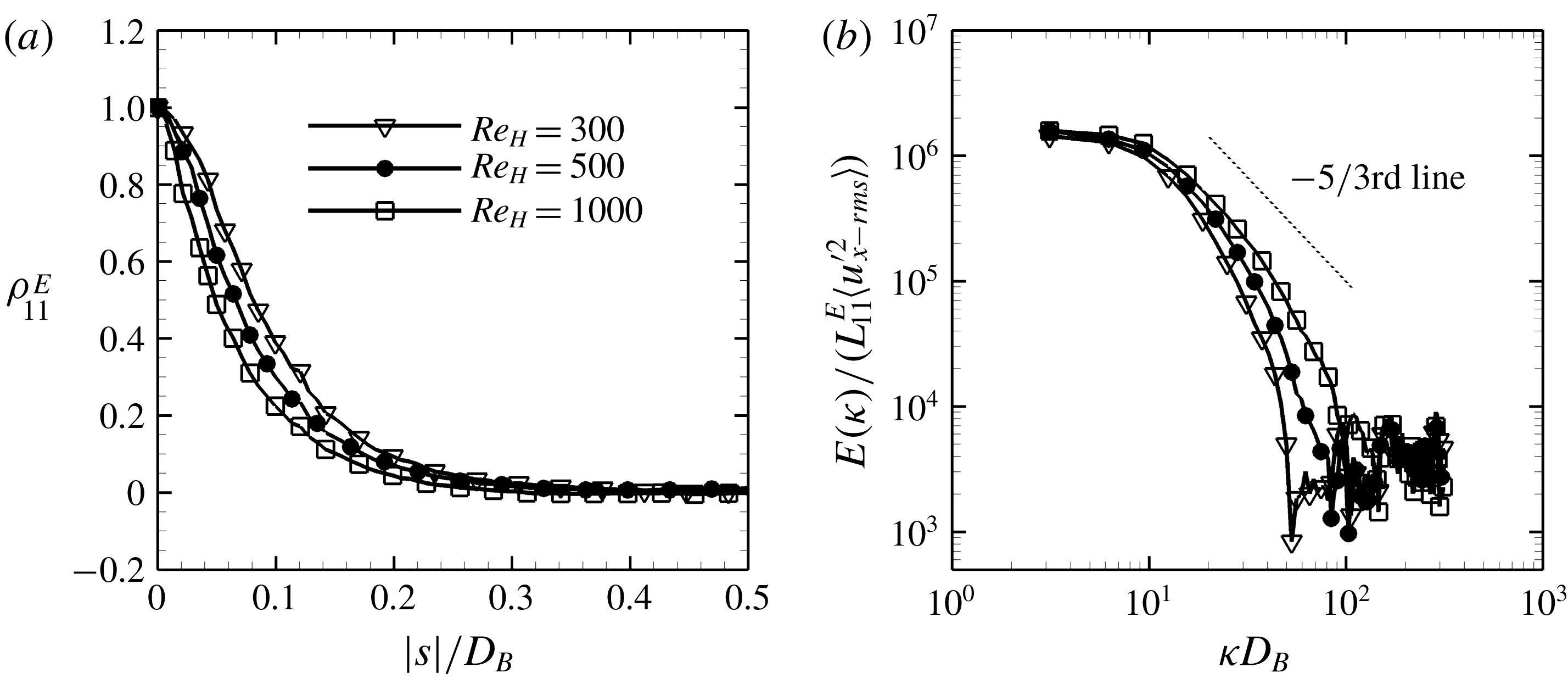
(a) Eulerian auto-correlations for different Reynolds number flows; (b) the corresponding energy spectra.

In figure 7(a), the auto-correlations computed with temporal fluctuating velocity component in
 $x$
-direction are plotted against the norm of the position vector
 $|\boldsymbol{s}|$
, non-dimensionalized by the particle diameter
 $D_{B}$
. The correlation near the origin drops off faster at higher
 $Re_{H}$
, indicating that the flow decorrelates more rapidly with distance at high Reynolds numbers than at low Reynolds numbers. The Eulerian integral length scales,
 $L_{11}^{E}$
, are calculated by integrating the correlations over the abscissa and the results are presented in table 3. The integral length scales decrease with increasing Reynolds number. Moreover, even for the lowest Reynolds number flow studied here, the integral length scale is only about 10 % of the particle diameter, indicating that the coherent structures are confined within the pore. This also shows that a single unit cell used as the computational domain in the present work is sufficient and does not affect the turbulence structures and characteristics. This was also confirmed by performing a simulation in a
 $3\times 3\times 3$
lattice on a coarser mesh and comparing the auto-correlations from two calculations which showed little difference even for the lowest
 $Re_{H}$
studied here.
These trends on integral length scale qualitatively agree with what was reported by Patil & Liburdy (Reference Patil and Liburdy2013), where a PIV measurement was carried out to determine the integral scales in different pores. Such observations also support the pore-scale prevalence hypothesis (known as PSPH) and are in agreement with the conclusion drawn by Jin et al. (Reference Jin, Uth, Kuznetsov and Herwig2015). Moreover, this suggests that, the turbulence at the pore-scale is strongly affected by the pore geometry. The solid phase in porous media breaks down the turbulence structures, and prohibits the presence of macroscopic turbulence structures that can span into multiple pores. This may be a result of the very low porosity and structured packing studied in the present work. Studies in random packings are needed to see if turbulence structures larger than pore size can be obtained. Also, this does not rule out the possibility that multi-pore-spanning turbulence structures may occur for higher porosity cases (Chu et al. Reference Chu, Weigand and Vaikuntanathan2018).
Eulerian integral length scales normalized by the particle diameter for different Reynolds numbers.

The energy spectra, calculated by applying the Fourier transform to the auto-correlations, are shown in figure 7(b). The spectra are normalized by the integral length scale and the r.m.s. fluctuating velocity in the
 $x$
-direction, so that the spectra have almost the same value at the smallest wavenumber for different Reynolds numbers. The wavenumber
 $\unicode[STIX]{x1D705}$
is also scaled by the particle diameter,
 $D_{B}$
. The well known Kolmogorov’s
 $-5/3$
rd law is distinguished by a dotted line in the figure. For the present studies,
 $Re_{H}$
is still small enough that distinct scale separation with inertial range is not clearly seen. For the highest Reynolds number studied (
 $Re_{H}=1000$
), a small region of the spectrum does show the
 $-5/3$
exponent. Similar behaviour was observed for angular multiscale statistics (He et al.
Reference He, Apte, Schneider and Kadoch2018). However, the presence of a broadband spectrum is observed indicative of turbulent flow within the pores. This suggests that the geometric confinement and highly tortuous flow obtained in such low porosity media does not significantly affect the energy cascade process. Similar observation was reported for high Reynolds number flows through a dilute porous system (Jin et al.
Reference Jin, Uth, Kuznetsov and Herwig2015).
Finally, Lagrangian time scales are estimated from the Eulerian statistics using a simple scaling model proposed by Corrsin (Reference Corrsin1963). This model suggests that, under assumptions of a homogeneous and stationary turbulent flow, the Lagrangian integral length scale would have roughly the same value as the Eulerian length scale. Consequently, the r.m.s. values of both Eulerian and Lagrangian fluctuation velocities should be of same magnitude. Tennekes & Lumley (Reference Tennekes and Lumley1972) summarized the model and suggested a scaling method
 $$\begin{eqnarray}\displaystyle T^{L}\approx \unicode[STIX]{x1D6FC}\frac{l_{pore}}{u_{x-rms}^{\prime }}, & & \displaystyle\end{eqnarray}$$
where
 $T^{L}$
is the Lagrangian integral time scale,
 $l_{pore}$
is a mixing or integral length scale, and
 $\unicode[STIX]{x1D6FC}$
is a coefficient. The coefficient
 $\unicode[STIX]{x1D6FC}$
is suggested to be in the range from
 $1/3$
to 3 (Tennekes & Lumley Reference Tennekes and Lumley1972) and may depend on the flow configuration and the Reynolds number. Patil & Liburdy (Reference Patil and Liburdy2013) applied the similar model to estimate the Lagrangian time scales and dispersion coefficients using their experimental data. They indicated that
 $l_{pore}$
can be taken as twice the Eulerian integral length scale. In our previous work on Lagrangian multiscale statistics of turbulent flows in the same geometry (He et al.
Reference He, Apte, Schneider and Kadoch2018), the values of the Lagrangian time scales have been estimated for the three Reynolds numbers studied in the current work. Thus, all parameters in (3.4) except
 $\unicode[STIX]{x1D6FC}$
have been obtained, and as a result the constant
 $\unicode[STIX]{x1D6FC}$
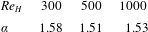
can be estimated directly, and is presented in table 4. It is evident that all
 $\unicode[STIX]{x1D6FC}$
values are in the range suggested by Tennekes & Lumley (Reference Tennekes and Lumley1972) and do not change significantly with Reynolds number. This implies that the model is, somewhat surprisingly, still valid even for the current setting of inhomogeneous flows. This finding does require that the computational volume chosen is representative, such that quantities computed no longer depend upon the domain size.
Coefficient
 $\unicode[STIX]{x1D6FC}$
in (3.4) for the Lagrangian time scale at different Reynolds number flows.

3.3 Velocity, vorticity and relative helicity statistics
The statistics of the instantaneous velocity (
 $\boldsymbol{u}$
), the vorticity (
 $\unicode[STIX]{x1D74E}$
) and the relative helicity (
 $\cos (\unicode[STIX]{x1D6F7})$
) were investigated in detail by computing the spatial variance and the probability density functions (p.d.f.s) for each Reynolds number. Hill & Koch (Reference Hill and Koch2002) conducted a similar spatial analysis for lower Reynolds numbers; and this facilitates comparisons with their work in understanding the differences among steady inertial, unsteady transitional and turbulent flows.
The relative helicity,
 $\cos (\unicode[STIX]{x1D6F7})$
, is defined by
 $$\begin{eqnarray}\displaystyle \cos (\unicode[STIX]{x1D6F7})=\frac{\unicode[STIX]{x1D74E}\boldsymbol{\cdot }\boldsymbol{u}}{|\unicode[STIX]{x1D74E}||\boldsymbol{u}|}, & & \displaystyle\end{eqnarray}$$
where
 $\unicode[STIX]{x1D74E}=\unicode[STIX]{x1D735}\times \boldsymbol{u}$
is the vorticity vector and is a measure of how well the velocity and vorticity vectors are aligned with each other. Helical motions are generated if the velocity and vorticity are well aligned. The spatial fluctuation of any field quantity
 $\unicode[STIX]{x1D713}$
is defined by
 $$\begin{eqnarray}\displaystyle \tilde{\unicode[STIX]{x1D713}}(\boldsymbol{x})=\unicode[STIX]{x1D713}(\boldsymbol{x})-\langle \unicode[STIX]{x1D713}\rangle ^{\unicode[STIX]{x1D6FE}}|_{\boldsymbol{x}}, & & \displaystyle\end{eqnarray}$$
where
 $\tilde{\unicode[STIX]{x1D713}}$
is the spatial fluctuation of
 $\unicode[STIX]{x1D713}$
. For the current study, the statistics, including the spatial p.d.f.s and variances, are first sampled in the fluid domain at multiple time instances for
 $10T_{f}$
, and then time-averaged.
3.3.1 Spatial variance
Following Hill & Koch (Reference Hill and Koch2002), the spatial variances for the instantaneous velocity (
 $R_{ij}$
) and vorticity (
 $O_{ij}$
) are defined as
 $$\begin{eqnarray}\displaystyle & \displaystyle R_{ij}(t)=\langle \tilde{u} _{i}\tilde{u} _{j}\rangle ^{\unicode[STIX]{x1D6FE}}/(\langle u_{x}\rangle ^{\unicode[STIX]{x1D6FE}})^{2}, & \displaystyle\end{eqnarray}$$
 $$\begin{eqnarray}\displaystyle & \displaystyle O_{ij}(t)=\langle \tilde{\unicode[STIX]{x1D714}}_{i}\tilde{\unicode[STIX]{x1D714}}_{j}\rangle ^{\unicode[STIX]{x1D6FE}}(D_{B}/2)^{2}/(\langle u_{x}\rangle ^{\unicode[STIX]{x1D6FE}})^{2}. & \displaystyle\end{eqnarray}$$
The streamwise and spanwise components of the variances are given by the diagonal part of
 $R_{ij}$
and
 $O_{ij}$
, which are defined as
 $$\begin{eqnarray}\displaystyle R_{||}=R_{11}\quad \text{and}\quad R_{\bot }=(R_{22}+R_{33})/2, & & \displaystyle\end{eqnarray}$$
 $$\begin{eqnarray}\displaystyle O_{||}=O_{11}\quad \text{and}\quad O_{\bot }=(O_{22}+O_{33})/2, & & \displaystyle\end{eqnarray}$$
where the subscript
 $\Vert$
represents streamwise and
 $\bot$
spanwise. As for the relative helicity
 $\cos (\unicode[STIX]{x1D6F7})$
, the variance
 $C$
is calculated as
 $$\begin{eqnarray}\displaystyle C(t)=\langle \cos ^{2}(\unicode[STIX]{x1D6F7})\rangle ^{\unicode[STIX]{x1D6FE}}-(\langle \cos (\unicode[STIX]{x1D6F7})\rangle ^{\unicode[STIX]{x1D6FE}})^{2}. & & \displaystyle\end{eqnarray}$$
Table 5 shows the time-averaged spatial variances for the velocities and vorticities in both streamwise and spanwise directions, as well as the relative helicity. A reasonable agreement of the variances at
 $Re_{H}=300$
is found between the current study and Hill & Koch (Reference Hill and Koch2002). The small differences may be attributed to (i) the time-averaging, which may have removed some of the temporal fluctuations and was not performed by Hill & Koch (Reference Hill and Koch2002), and (ii) the grid resolution, which was much coarser in Hill & Koch (Reference Hill and Koch2002) so that some very small velocities near the solid wall may not be completely resolved in their work.
Time-averaged spatial variances of velocity and vorticity in the streamwise and spanwise directions together with the relative helicity at three different Reynolds numbers; the overbar means time-averaging; the first line are the data reported by Hill & Koch (Reference Hill and Koch2002) at the same Reynolds number of
 $Re_{H}=300$
at one time instant.

Table 5 indicates that the variance values for velocity in the streamwise direction are smaller than that in the spanwise directions. This is attributed to the fact that the mean flow is strong in the streamwise direction, while almost zero in the other directions. For the vorticity components in both streamwise and spanwise directions, the variances are increasing almost linearly with
 $Re_{H}$
, and the values are essentially equal regardless of the direction. This is quite different for the steady inertial and weakly turbulent flows reported in Hill & Koch (Reference Hill and Koch2002). They observed that the variance of vorticity in spanwise directions is much larger than that in the streamwise direction. For steady inertial flows, the vortices are primarily initiated by shear close to the particle surfaces. Thus the cross-flow components are much stronger. For the unsteady flows, however, vortex shedding becomes important, stretching the flow structures and initiating the generation of vortices in all directions, even away from the solid surface. In the fully turbulent flows, this mechanism is greatly magnified. Finally, the variance of relative helicity roughly remains constant for the high Reynolds number turbulent flows studied here. This is also distinctly different compared to the observations of Hill & Koch (Reference Hill and Koch2002). They reported that the variance increases greatly from the Darcy flow regime to the unsteady flow regime. To understand the above trends better, the p.d.f.s of velocity, vorticity and relative helicity are computed and plotted below.
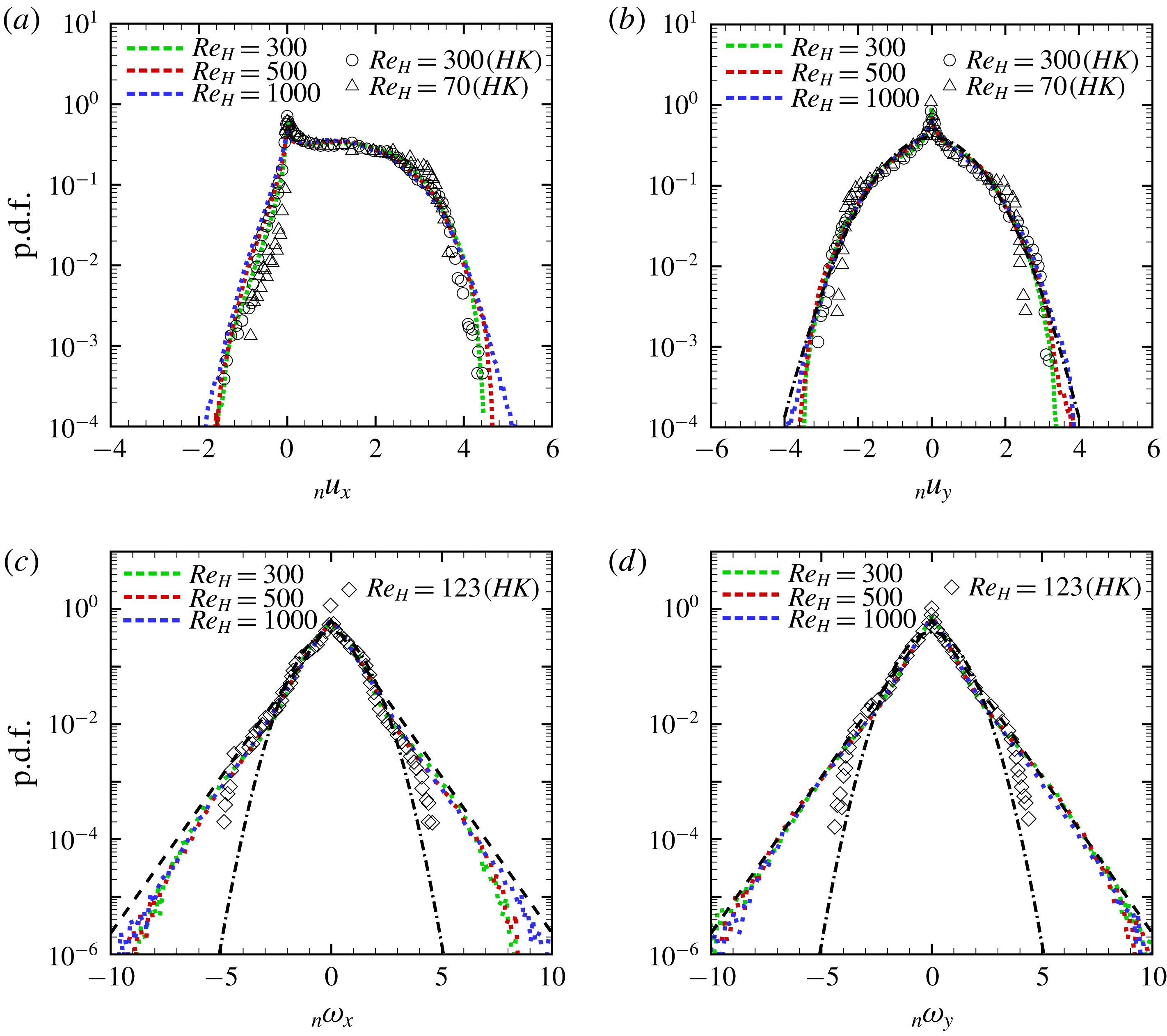
The normalized p.d.f.s for velocity and vorticity for different Reynolds numbers: (a)
 $x$
-component of velocity, (b)
 $y$
-component of velocity, (c)
 $x$
-component of vorticity, and (d)
 $y$
-component of vorticity. The dotted green line is for
 $Re_{H}=300$
, red
 $Re_{H}=500$
and blue
 $Re_{H}=1000$
. Here ○, ♢, and ▵ denote the data from Hill & Koch (Reference Hill and Koch2002) for
 $Re_{H}=300$
,
 $123$
, and
 $70$
, respectively. The black dash-dot line represents the Gaussian distribution with zero mean and unit standard deviation. The black dashed line stands for the double-exponential distribution.

3.3.2 Probability density functions
The normalized probability density functions for the velocities, vorticities and relative helicity are provided in this section. The spatial variances in table 5 are used to normalize the p.d.f.s making their standard deviations unity and allowing direct comparison with the Gaussian or double exponential distributions. For the plots in this section, the subscript ‘n’ in the titles of the abscissas, for example
 $\text{}_{n}u_{x}$
, means that the abscissa has been normalized by its spatial variance. Owing to the periodicity, the statistics in the
 $y$
- and
 $z$
-directions should be the same (which was verified) and hence only the p.d.f.s of velocity in the
 $y$
-direction are shown.
The p.d.f.s for the instantaneous velocity and vorticity components in the streamwise and spanwise directions are given in figure 8 for the three Reynolds numbers. Data from Hill & Koch (Reference Hill and Koch2002) is also included for the lower Reynolds number steady inertial or weakly turbulent flows for comparison. It can be observed that the p.d.f.s for lowest Reynolds number of
 $300$
studied in the present work are in reasonable agreement for the corresponding p.d.f.s from Hill & Koch (Reference Hill and Koch2002).
The p.d.f.s for velocities seem to have similar behaviour over a range of Reynolds numbers after proper normalization. This suggests that, at least in the sense of the first order statistics, the main topology does not change much with respect to the Reynolds number, which agrees qualitatively with the observation in § 3.1.1. Consistent with observations of Hill & Koch (Reference Hill and Koch2002), more
 $x$
-component velocities in the upstream direction are detected for higher
 $Re_{H}$
. This can be seen at the right tails of p.d.f.s especially in figure 8(a). The stronger recirculation, as well as the large number of vortices generated with one of the components perpendicular to the
 $x$
-direction, are potentially responsible for this observation. In addition, a near-exponential decay (at a rate faster than the Gaussian distribution) is observed at the right-hand side tail of the velocity p.d.f.s, especially for lower Reynolds numbers; and the decaying rate is closer to the Gaussian distribution at higher Reynolds numbers. The p.d.f.s of instantaneous velocities shown in figure 8(b) generally follow the Gaussian distribution until about three times the standard deviation in both positive and negative abscissas, then continue to decay, but at rates noticeably larger than the Gaussian function. This indicates that the decay rates of the tails of the velocity field are Reynolds-number-dependent for the range considered in the present study. Hill & Koch (Reference Hill and Koch2002) conjectured that the exponential decay at lower Reynolds numbers is because of the distribution of the pore size and is not dependent upon the Reynolds number. However, as is shown in the present study, with increasing Reynolds numbers, the flow structures and length scales become smaller even in the main flow direction. This isotropization of the velocity field at higher
 $Re_{H}$
is probably the cause of the more Gaussian-distributed p.d.f.s observed.
The p.d.f.s for the vorticity components in the
 $x$
- and
 $y$
-directions for different Reynolds numbers are shown in figures 8(c) and 8(d), respectively. The p.d.f.s for steady inertial flow at
 $Re_{H}=123$
(♢) from Hill & Koch (Reference Hill and Koch2002) is also shown for comparison. It can be observed that the p.d.f.s for the turbulent flows studied in the present work are quite different from those for the steady inertial flow reported in Hill & Koch (Reference Hill and Koch2002). For the turbulent flows, the p.d.f.s for
 $\text{}_{n}\unicode[STIX]{x1D714}_{x}$
are almost decaying exponentially until about five times the standard deviation regardless of
 $Re_{H}$
. This trend is even more pronounced for the p.d.f.s of the vorticities in the spanwise directions, which follow the double exponential function till about seven times the standard deviation. While for Hill and Koch’s steady inertial flow, the p.d.f.s first follow the double exponential distribution until about three times the standard deviation, then start to decay in a rate closer to the Gaussian function. Such near-Gaussian decay is almost entirely absent from any of the unsteady flows studied in the current work.
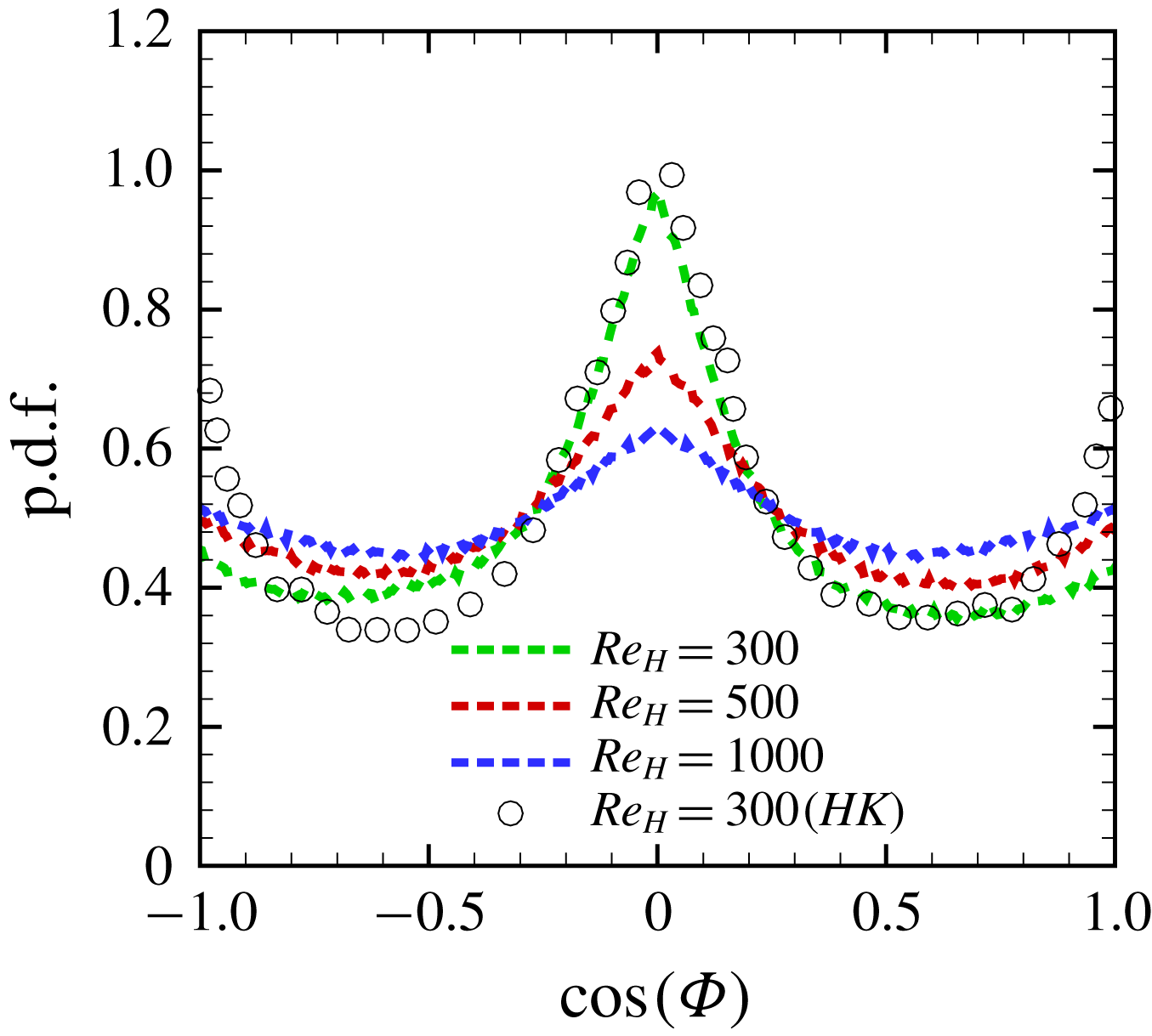
The p.d.f. of normalized relative helicity. The dotted green line is for
 $Re_{H}=300$
, red
 $Re_{H}=500$
and blue
 $Re_{H}=1000$
; ○ illustrate the data from Hill & Koch (Reference Hill and Koch2002) for
 $Re_{H}=300$
.

Finally, the p.d.f.s for the relative helicity are displayed in figure 9. Note that the abscissa of figure 9 has not been scaled by the standard deviation because the p.d.f.s for relative helicity are periodic with respect to the angle (
 $\unicode[STIX]{x1D6F7}$
). At
 $Re_{H}=300$
, there is a distinct peak in the p.d.f. at
 $\cos \unicode[STIX]{x1D6F7}=0$
, indicating that the vorticity and velocity vectors are not aligned for the majority of the flow region. Comparing the p.d.f.s for
 $\cos \unicode[STIX]{x1D6F7}$
at
 $Re_{H}=300$
from the current study and Hill & Koch (Reference Hill and Koch2002), some deviations could be observed, especially at large magnitude of
 $\cos \unicode[STIX]{x1D6F7}$
. This difference could be due to the fact that the p.d.f. reported in Hill & Koch (Reference Hill and Koch2002) is only at one time instant, while it has been time-averaged in the present study. Unlike the velocity and vorticity, the p.d.f.s of relative helicity are strongly dependent on the Reynolds number. It can be observed from figure 9 that higher Reynolds-number flows tend to have higher probability of smaller angles between the velocity and vorticity vectors, aligning them to create helical structures. It indicates the mechanism by which the turbulent kinetic energy is transferred from large to small scale structures by helical motions and stretching.
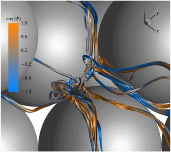
Figure 10 shows instantaneous stream-ribbons coloured by the relative helicity for
 $Re_{H}=1000$
. It is observed that substantial helicity is generated in the initial part of the centre pore and propagated downstream, where the stream ribbons are coloured either by orange (
 $\cos (\unicode[STIX]{x1D6F7})=1$
) or blue (
 $\cos (\unicode[STIX]{x1D6F7})=-1$
), confirming the alignment of velocity and vorticity. With such alignment, the vorticity is advected downstream in the streamwise direction by the velocity giving rise to the helical motions.
Instantaneous stream ribbons coloured by the relative helicity (
 $\cos (\unicode[STIX]{x1D6F7})$
) of flow through the centre pore for
 $Re_{H}=1000$
(mean flow is in the positive
 $x$
-direction).

3.4 The velocity gradient tensor and anisotropy characteristics
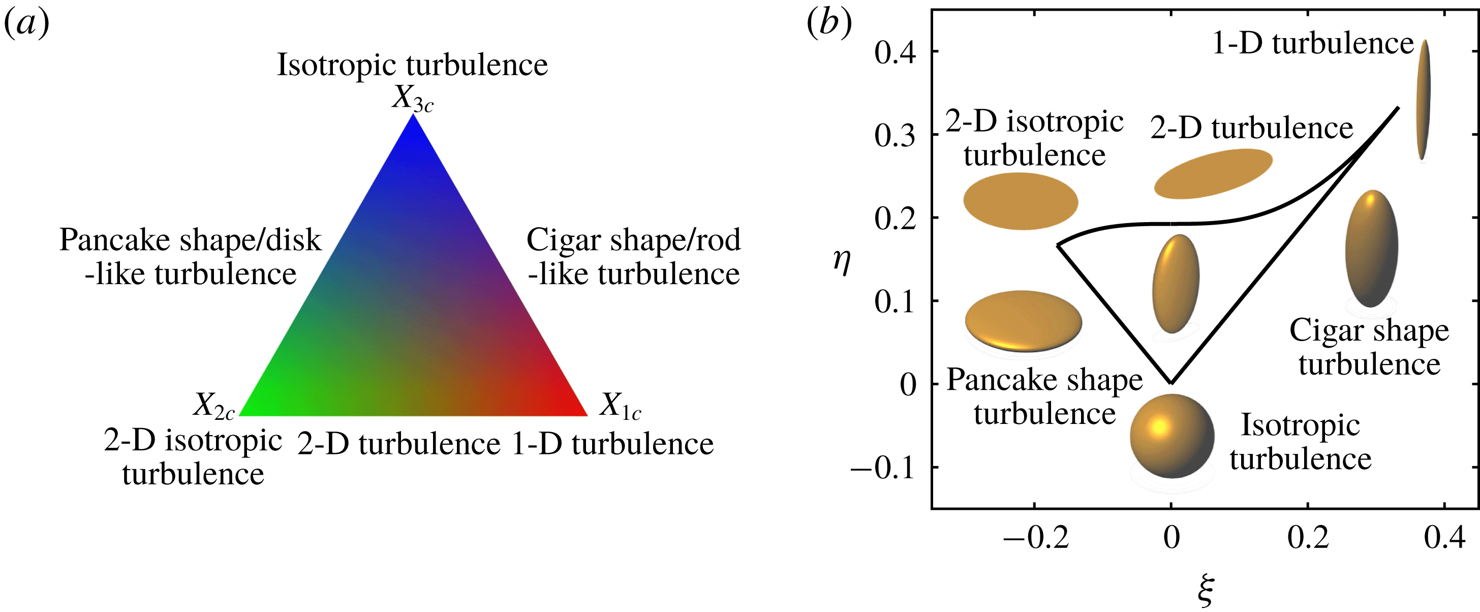
In this section, the velocity gradient tensor and its properties are first used to visualize the vortical structures. Then, the anisotropy characteristics are illustrated using the barycentric componentality contour mapping and the characteristic spheroids methods. Finally, the invariant space based on the velocity gradient tensor is used to identify different flow regimes within the pore.
3.4.1 Vortical structure visualization
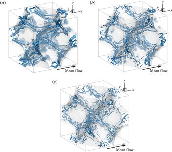
To inspect how the vortical structures are influenced by inertia effects, the local swirling strength
 $\unicode[STIX]{x1D706}_{ci}$
is used to visualize the flows at different
 $Re_{H}$
as shown in figures 11(a), 11(b) and 11(c). The field variable
 $\unicode[STIX]{x1D706}_{ci}$
is determined by computing the imaginary component of the complex conjugate eigenvalue of the velocity gradient tensor
 $\unicode[STIX]{x1D608}_{ij}$
(Zhou et al.
Reference Zhou, Adrian, Balachandar and Kendall1999), defined as
 $$\begin{eqnarray}\displaystyle \unicode[STIX]{x1D608}_{ij}=\unicode[STIX]{x2202}u_{i}/\unicode[STIX]{x2202}x_{j}. & & \displaystyle\end{eqnarray}$$
The isosurfaces in these figures were set at 25 % of the local maximum value of
 $\unicode[STIX]{x1D706}_{ci}$
. With increasing
 $Re_{H}$
, the size of vortical structures becomes smaller. These structures seem to be stretched and aligned in the streamwise mean flow direction at lower
 $Re_{H}$
, however, and are broken down into much smaller structures at higher Reynolds numbers. For the cases studied in the present work, the size of these flow structures are still much smaller than the particle size. Thus, the turbulence is expected to be confined to the microscales of pores, as discussed in § 3.2. The size and connectivity of vortical structures located at distinct parts of unit cell are quite different for the different Reynolds numbers examined, suggesting a highly anisotropic flow field. To assess this further, the Reynolds stress anisotropy tensor is computed and its characteristics are analysed in the following section.
The isosurface of the swirling strength at
 $\unicode[STIX]{x1D706}=0.25\unicode[STIX]{x1D706}_{max}$
. (a) is for
 $Re_{H}=300$
, (b)
 $Re_{H}=500$
and (c)
 $Re_{H}=1000$
.

3.4.2 Anisotropy characteristics
The anisotropy in the Reynolds stress distribution in the pore is important for understanding both the dynamics of the turbulent motions and the kinetic energy transport mechanism within the pore space. It is conventionally characterized by the normalized Reynolds stress anisotropy tensor,
 $\unicode[STIX]{x1D623}_{ij}$
, defined as
 $$\begin{eqnarray}\displaystyle \unicode[STIX]{x1D623}_{ij}=\frac{\unicode[STIX]{x1D622}_{ij}}{2k}=\frac{\overline{u_{i}^{\prime }u_{j}^{\prime }}}{\overline{u_{k}^{\prime }u_{k}^{\prime }}}-\frac{1}{3}\unicode[STIX]{x1D6FF}_{ij}. & & \displaystyle\end{eqnarray}$$
Here,
 $\unicode[STIX]{x1D6FF}_{ij}$
is the Kronecker delta tensor and
 $k$
is the turbulent kinetic energy. The invariants of the tensor
 $\unicode[STIX]{x1D623}_{ij}$
are related to its three eigenvalues,
 $\unicode[STIX]{x1D706}_{i}$
. In particular, the second (
 $II=3\unicode[STIX]{x1D702}^{2}$
) and third (
 $III=2\unicode[STIX]{x1D709}^{3}$
) invariants associated with
 $\unicode[STIX]{x1D623}_{ij}$
can be computed from
 $$\begin{eqnarray}\displaystyle \displaystyle II=3\unicode[STIX]{x1D702}^{2} & = & \displaystyle b_{ji}\unicode[STIX]{x1D623}_{ij}/2\nonumber\\ \displaystyle & = & \displaystyle \unicode[STIX]{x1D706}_{1}^{2}+\unicode[STIX]{x1D706}_{1}\unicode[STIX]{x1D706}_{2}+\unicode[STIX]{x1D706}_{2}^{2}\end{eqnarray}$$
 $$\begin{eqnarray}\displaystyle \displaystyle III=2\unicode[STIX]{x1D709}^{3} & = & \displaystyle \unicode[STIX]{x1D623}_{ij}\unicode[STIX]{x1D623}_{jn}\unicode[STIX]{x1D623}_{ni}/3\nonumber\\ \displaystyle & = & \displaystyle -\unicode[STIX]{x1D706}_{1}\unicode[STIX]{x1D706}_{2}(\unicode[STIX]{x1D706}_{1}+\unicode[STIX]{x1D706}_{2}),\end{eqnarray}$$
where
 $\unicode[STIX]{x1D702}$
characterizes the degree of anisotropy and
 $\unicode[STIX]{x1D709}$
describes its characteristic shape. These invariants are routinely used to compose the coordinate system to illustrate the anisotropy, for example, Lumley triangle (Lumley & Newman Reference Lumley and Newman1977) and turbulence triangle (Choi & Lumley Reference Choi and Lumley2001). These are both nonlinear invariant maps, but the first one is constructed based on the invariants
 $II$
and
 $III$
of
 $\unicode[STIX]{x1D623}_{ij}$
, and the second on the same invariants but in the transformed coordinate system
 $(\unicode[STIX]{x1D709},\unicode[STIX]{x1D702})$
. These maps are very useful, especially for the geometrically simple scenarios such as the turbulent channel flow. However, when dealing with a complex flow field, since the physical coordinate information is lost, they fail to identify the local region to which the anisotropic characteristics belong. In addition, they are appropriate only for visualizing small amounts of data (Emory & Iaccarino Reference Emory and Iaccarino2014).
For the current study, the barycentric componentality contour map developed by Emory & Iaccarino (Reference Emory and Iaccarino2014) is applied to diminish the drawbacks of the nonlinear invariant maps. Componentality maps are combinations of the eigenvalues that help characterize the topology of turbulence. In short, the limiting values of componentality can be thought of as being 1-component (roughly like a needle), 2-component (flat disk-like), or 3-component (roughly spherical). Using componentality, the anisotropy can be graphically visualized. This approach is briefly described as follows.
The barycentric map, first introduced by Banerjee et al. (Reference Banerjee, Krahl, Durst and Zenger2007), utilizes the fact that all the turbulence states with physical meanings should be bounded by the three limiting states of componentality (described above) in a convex combination. Thus, a Euclidian domain in an equilateral triangle, where the three limiting states with equal weights are placed at
 $\boldsymbol{x}_{1c}=(1,0)$
,
 $\boldsymbol{x}_{2c}=(0,0)$
and
 $\boldsymbol{x}_{3c}=({\textstyle \frac{1}{2}},\sqrt{3}/2)$
(see figure 12
a) can be established. The corresponding coordinate system
 $(x_{B},y_{B})$
in the map can be written as
 $$\begin{eqnarray}\displaystyle & \displaystyle x_{B}=C_{1c}x_{1c}+C_{2c}x_{2c}+C_{3c}x_{3c}, & \displaystyle\end{eqnarray}$$
 $$\begin{eqnarray}\displaystyle & \displaystyle y_{B}=C_{1c}y_{1c}+C_{2c}y_{2c}+C_{3c}y_{3c}, & \displaystyle\end{eqnarray}$$
where the weights
 $C_{ic}$
are defined as
 $$\begin{eqnarray}\displaystyle & \displaystyle C_{1c}=\unicode[STIX]{x1D706}_{1}-\unicode[STIX]{x1D706}_{2}, & \displaystyle\end{eqnarray}$$
 $$\begin{eqnarray}\displaystyle & \displaystyle C_{2c}=2(\unicode[STIX]{x1D706}_{2}-\unicode[STIX]{x1D706}_{3}), & \displaystyle\end{eqnarray}$$
 $$\begin{eqnarray}\displaystyle & \displaystyle C_{3c}=3\unicode[STIX]{x1D706}_{3}+1. & \displaystyle\end{eqnarray}$$
Note that any
 $C_{ic}$
resides in the range
 $[0,1]$
. This setting is coincident with the red-green-blue (RGB) colour system, where the
 $[1,0,0]$
is coded for red,
 $[0,1,0]$
green, and
 $[0,0,1]$
blue. Every colour could be expressed by a linear combination of these three triplets. As a result, the barycentric componentality coefficients
 $C_{ic}$
could as well be used as the coefficients for the RGB colour function in the form of
 $$\begin{eqnarray}\displaystyle \left[\begin{array}{@{}c@{}}R\\ G\\ B\end{array}\right]=C_{1c}\left[\begin{array}{@{}c@{}}1\\ 0\\ 0\end{array}\right]+C_{2c}\left[\begin{array}{@{}c@{}}0\\ 1\\ 0\end{array}\right]+C_{3c}\left[\begin{array}{@{}c@{}}0\\ 0\\ 1\end{array}\right]\!. & & \displaystyle\end{eqnarray}$$
Therefore, the different shapes of turbulence can be mapped onto the equilateral triangle (see figure 12 a) with the help of the RGB colour system. In particular, one-dimensional turbulence is identified by red, two-component turbulence by green, and the isotropic turbulence by the colour blue.
(a) Reynolds stress anisotropy componentality contour in the barycentric colour map. (b) Lumley triangle showing limits of the invariants
 $\unicode[STIX]{x1D709}$
and
 $\unicode[STIX]{x1D702}$
and characteristic spheroids representing the shape of the turbulence.

The column on the left-hand side shows the contours for anisotropy at the centre slice using barycentric componentality map; and the right-hand side illustrates the anisotropy by the characteristic ellipsoids with a zoom-in view at the centre pore (the dashed square in (a)): (a,b)
 $Re_{H}=300$
, (c,d)
 $Re_{H}=500$
, and third (e,f)
 $Re_{H}=1000$
.

Distribution of the anisotropy stress tensor on the centre
 $xy$
-slice of the porous unit cell described by the barycentric componentality contour map is shown in figures 13(a), 13(c) and 13(e) for the three Reynolds numbers, respectively. In addition, a new technique, first introduced by Hamilton & Cal (Reference Hamilton and Cal2015), is applied as well to visualize the turbulence structures more intuitively. The algorithm involves using the eigenvalue decomposition of the normalized Reynolds stress anisotropy tensor to extract the corresponding eigenvalues and eigenvectors. The characteristic triaxial ellipsoids (figure 12
b), with the shape determined by the eigenvalues and orientation by the eigenvectors, can then be drawn to directly represent the turbulence structure as described by Lumley triangle. Figures 13(b), 13(d) and 13(f) provide zoom-in views on the centre pore region (shown as the dashed square in figure 13
a) depicting the turbulence with such ellipsoids. Note, in order to avoid the clustering, only one in six of the data points in each direction are displayed.
Figures 13(a), 13(c) and 13(e) show that some characteristics of the anisotropy stress tensor are common to all three Reynolds-number flows. The characteristic ellipsoids in figures 13(b), 13(d) and 13(f) help to visualize the types of structures present in different regions. Firstly, in the regions close to the contact points of the spheres on the left-hand side, the near one-dimensional turbulence (red-ish) dominates as the flow is squeezed and accelerated by the particles to form a jet-like structure. At higher Reynolds numbers, the extent of this one-dimensional turbulence is reduced. As the accelerated flow extends into the pore space, transition to 2-D turbulence (green) is observed. A weak wake-like region is present behind the left sphere. In the regions of peak TKE production (yellow-dashed circles in figures 13
a, 13
c and 13
e), the boundary between red (one-dimensional (1-D) turbulence) and green (2-D turbulence) becomes less discernible with increasing
 $Re$
. The dominant colour transits from light red-ish (figure 13
a,
 $Re_{H}=300$
), to a mixture of green and red (figure 13
c,
 $Re_{H}=500$
) and finally turns to purple-ish (figure 13
e,
 $Re_{H}=1000$
). Moreover, the ellipsoids in the red-dashed circles in figures 13(b), 13(d) and 13(f) indicate that the shape of the turbulence becomes more like a 2-D disk when the Reynolds number increases from 300 to 500; and then develops into the cigar shape at
 $Re_{H}=1000$
. The flow squeezed through the boundaries of the particles is stretched mainly by the Reynolds stress in the main flow direction giving rise to cigar-shaped structures, whereas near the centre of the pore and on the left side, the structures are more stretched by other components of the Reynolds stress leading to the 2-D turbulence. The anisotropy distribution depends on the distance from the wall, as expected. Similar to duct flows, near-wall shear leads to higher anisotropy and elongated structures. However, in the present configuration, this phenomenon is not as pronounced owing to the three-dimensional geometry of the pore and the tortuous path of the flow through the FCC packing.
As the flow from the two corners of the left sphere meets near the centre of the pore, one transitions from 2-D (green-ish) to isotropic turbulence (blue). The extent of this isotropic region increases with increasing Reynolds number. This is also evident by small spherical shapes in the centre pore region towards the right-hand side. As the flow then impinges on the right sphere boundary, a region of disk-like structure is observed representing the isotropic 2-D turbulence (green region) very close to the particle surface. The anisotropy characteristics close to the stagnation zone is consistent with the results reported by Nishino et al. (Reference Nishino, Samada, Kasuya and Torii1996). As the flow turns and exits through the right corners, it is again squeezed to give the 1-D (red region) turbulence.
3.4.3
 $Q-R$
invariants space

The velocity gradient tensor has been thoroughly studied because it contains enriched geometric and statistical information of the flowfield, such as shapes of fluid volume, rate of deformation and intermittency (Meneveau Reference Meneveau2011). Particularly, much attention has been paid to the second and third invariants (Cantwell Reference Cantwell1992; Martin et al. Reference Martin, Ooi, Chong and Soria1998), defined based on this second order, traceless tensor as
 $$\begin{eqnarray}\displaystyle & \displaystyle Q=-{\textstyle \frac{1}{2}}\unicode[STIX]{x1D608}_{im}\unicode[STIX]{x1D608}_{mi}, & \displaystyle\end{eqnarray}$$
 $$\begin{eqnarray}\displaystyle & \displaystyle R=-{\textstyle \frac{1}{3}}\unicode[STIX]{x1D608}_{im}\unicode[STIX]{x1D608}_{mn}\unicode[STIX]{x1D608}_{ni}. & \displaystyle\end{eqnarray}$$
It is convenient to study the velocity gradient tensor through the investigation of two such invariants because, firstly, this methodology greatly reduces the dimension of the problem (from eight to two); and secondly, it can provide a representation of the local topology of fluid motion. One common observation among different types of turbulence is the sheared ‘tear drop’ shape distribution of the
 $(R,Q)$
-space (see Chong, Perry & Cantwell (Reference Chong, Perry and Cantwell1990), Cantwell (Reference Cantwell1993)). Also, there exists a distinguished line, the Vieillefosse tail defined as
 $Q=-(3/2^{2/3})R^{2/3}$
, along which the higher probability of data points are clustered especially at the
 $R>0$
and
 $Q<0$
quadrant. The Vieillefosse tail separates the
 $(R,Q)$
-space into two parts. The one above the curve represents the focal or vortical fluid motions and the other, below the curve, denotes the non-focal, dissipative motions. In this section, the
 $(R,Q)$
-space is examined for different regions in the pore based on the anisotropy distribution illustrated in § 3.4.2.
Scatter plots of the
 $(R,Q)$
-space at
 $Re_{H}=1000$
corresponding to data taken from different regions within the pore indicated in figure 13(f): (a) isotropic region corresponding to the green triangle area, (b) 2-D turbulence within the blue rectangle region, and (c) cigar-shaped turbulence structures corresponding to peak TKE production region represented by the two red circles. The dashed curves are the Vieillefosse tail.

The
 $(R,Q)$
-space scatter plots are shown in figure 14 for the highest Reynolds number
 $Re_{H}=1000$
. Data points from three different regions in figure 13(f), corresponding to the isotropic (green-dashed triangle), 2-D turbulence (blue-dashed rectangle) and cigar-shaped turbulence structures (red-dashed circles), which is also a region of high production of turbulent kinetic energy in figure 4(e), are used to draw figures 14(a), 14(b) and 14(c), respectively. The sheared ‘tear drop’ shape distribution of the
 $(R,Q)$
-space is generally recognized for all three regions and the Vieillefosse tail is followed in the
 $R>0$
and
 $Q<0$
quadrant. This is consistent with extensive observations of different types of turbulence observed from both numerical (Nomura & Post Reference Nomura and Post1998; Ooi et al.
Reference Ooi, Martin, Soria and Chong1999; Lüthi, Tsinober & Kinzelbach Reference Lüthi, Tsinober and Kinzelbach2005) and experimental (Gultitski et al.
Reference Gultitski, Kholmyansky, Kinzelbach, Luthi, Tsinober and Yorish2007; Elsinga & Marusic Reference Elsinga and Marusic2010) work. However, there are discrepancies in the scatter plots for the three regions depicted. The most noticeable difference is that considerably more data points above the Vieillefosse tail at the
 $R<0$
and
 $Q>0$
quadrant are observed for 2-D and cigar-shape turbulence, meaning that more vortical motions are present in these two regions. The fluid motions represented by the cigar-shape turbulence are mostly helical motions, which aggressively promote the production of TKE (see figure 4). Whereas for the isotropic turbulence region, the data points in the
 $(R,Q)$
-space are mostly clustered near the origin and follow the Vieillefosse tail in the
 $R>0$
and
 $Q<0$
quadrant, as expected. On the other hand, only small differences in data under the Vieillefosse tail are observed. As discussed in § 3.1.3, the TKE production peaks in particular regions within the pore; however, the dissipation rate of TKE is mostly non-zero over the entire pore space. This explains why there are little deviations of data points in the
 $(R,Q)$
-space below the Vieillefosse tail in different regions.
4 Summary
Pore-scale, fully resolved, direct numerical simulations were performed in a unit cell of a face-centred cubic lattice at three different Reynolds numbers (300, 500 and 1000), covering the transitional, unsteady inertial flow to the fully turbulent flow in porous media. A triply periodic domain is used and the flow is driven by an imposed pressure gradient in the axial direction. Fundamental characteristics of the flow topology, turbulent kinetic energy transport, scales of turbulence and anisotropy distribution at different Reynolds numbers were investigated in detail. Emphasis was placed on investigating how turbulence scales and energy transfer mechanisms are affected by the confined geometries of a low porosity (
 $\unicode[STIX]{x1D719}=0.26$
) medium. This study extends the work by Hill & Koch (Reference Hill and Koch2002) in the same configuration at lower Reynolds numbers, corresponding to steady inertial and unsteady, weakly turbulent flows, to the present fully turbulent flows in porous media. The main observations of this work are summarized below:
(i) Owing to the low porosity and resultant tortuous nature of the porous geometry, the mean flow in the axial direction exhibits strong acceleration and deceleration regions. The mean flow takes a highly tortuous path with the presence of three-dimensional helical motions, weak wake-like flow structures behind spheres, stagnation flow, jet impingement with the sphere boundary, as well as merging and spreading of jets.
(ii) The integral length scales of turbulence decrease with increasing Reynolds number and are found to be much smaller than the solid particle diameter of the pore (
 ${<}10\,\%$
). The turbulence structures are broken down by the confined boundaries, and hence macroscopic turbulence and flow structures, with sizes comparable to or larger than the pore size, were not observed. This result is consistent with the experimental and numerical data reported in Patil & Liburdy (Reference Patil and Liburdy2013) and Jin et al. (Reference Jin, Uth, Kuznetsov and Herwig2015), respectively. It also indicates that the volume-averaged, upscaled flow quantities may be confined to the representative volume of averaging. This is also confirmed by using the simple scaling model estimating Lagrangian time scales from the Eulerian statistics. This is attributed to the low porosity as well as the structured configuration studied here. Studies in random packings are necessary to further confirm that this is solely an effect of low porosity.
(iii) The peak value of turbulence intensity, and the spatial extent within the pore over which it occurs, increase with increasing Reynolds numbers. Unlike a confined duct flow with planar or complex wall shapes, the turbulence intensity levels in the main flow direction and cross-stream directions are of the same order, with the axial component somewhat lower than those in the cross-stream directions. This is a unique feature of the flow studied in the present work and is mainly attributed to the three-dimensional, tortuous path of the mean flow.
(iv) The probability density functions of cross-stream velocity show only a weak dependence on Reynolds number. However, p.d.f.s of vorticity followed a double exponential decay for turbulent flows at higher
 $Re_{H}$
, rather than a more Gaussian distribution as observed by Hill & Koch (Reference Hill and Koch2002) in their work on steady inertial flows. Strong dependence on Reynolds number is observed in p.d.f.s of relative helicity. Alignment of velocity and vorticity vectors over a large region within the pore is observed, leading to a more uniform p.d.f. for the relative helicity. This also suggests that with increasing
 $Re_{H}$
, formation of three-dimensional helical motions within the pore is more pronounced.
(v) The region of peak production of turbulent kinetic energy in the pore is observed to be behind the particles near the entrance with high mean shear. However, the dissipation rate of TKE is higher on the particle surfaces and remains high over most of the pore region. In addition, owing to large turbulence intensities in the entire pore, the contribution of the turbulent transport to the TKE budget is found to be important. Except the small regions near the peak of TKE production, production and dissipation are not balanced and thus the overall turbulence in the pore is not in equilibrium. Negative values of net production of TKE are observed in the jet impingement region, as well as in the weak-wake region behind the particle surfaces. The spanwise components of the production term become negative and outnumber the axial positive component, leading to a negative net production, a unique flow feature observed in the present configuration. The mean flow acceleration and deceleration are mainly responsible for the negative production of TKE, which is present over about 10 % of the volume of the pore region.
(vi) The flow and turbulence structures are illustrated by focusing on the velocity gradient and Reynolds stress tensors. The local swirl strength was computed from the velocity gradient tensor to visualize the vortical structures. Flow structures are found to be stretched and aligned in the streamwise mean flow direction at lower
 $Re_{H}$
; however, they break into much smaller structures at higher flow rates, suggesting a highly anisotropic flow field. Then, the anisotropy characteristics are studied by using the barycentric componentality map as well as the triaxial ellipsoids, identifying isotropic, cigar-shaped and 2-D turbulence regimes and transitions between them within the pore. A one-dimensional turbulence region is observed in corner regions of the pore where the flow is squeezed through two or more particle surfaces. This 1-D turbulence transitions to 2-D turbulence within the weak, wake-like region in the pore behind the particle surface. An isotropic region is also observed before the stagnation point of the jet-impingement-like flow which exhibits disk-like structures. In the regions of peak production, a transition from 2-D to cigar-shaped turbulence structures was observed. In this region, the velocity and vorticity vectors are highly aligned creating helical structures. This is also verified by the scatter plot of
 $(R,Q)$
-space which gives more data points above the Vieillefosse tail, confirming presence of more vortical/helical structures that promote production of TKE.
(vii) Finally, the characteristics of mean velocity and turbulence statistics for flow through porous media are complex even for the structured packing studied here. These flow features do not really correspond to internal duct-like flow, even for ducts with complex shaped boundaries. Several differences such as higher turbulence intensities in the spanwise directions compared to the main flow direction, as well as much higher level of turbulence kinetic energy in the centre region were observed. The flow characteristics also do not correspond to external flow over spherical structures as large-scale vortex shedding and wake regions were absent especially in the low porosity configuration studied here. Complex flow patterns involving jet-impingement against the particle walls, recirculation regions and jet interactions were observed.
Acknowledgements
The authors acknowledge the use of computational resources from the Texas Advanced Computing Center at The University of Texas at Austin. This work was funded in part by NSF award 1336983. X.H. gratefully thanks Dr N. Hamilton (National Renewable Energy Laboratory, Boulder, CO) for providing the source code for visualizing anisotropy using the characteristic ellipsoids. S.V.A. acknowledges fruitful discussions with several researchers during the Center for Turbulence Research’s Summer Program at Stanford University.
Nomenclature
Operator:
-
$\langle \,\cdot \,\rangle$
volume averaging operator
-
$\overline{~\cdot ~}$
temporal averaging operator
-
$\langle \,\cdot \,\rangle _{A}$
area averaging operator


Subscript/superscript:
-
$\unicode[STIX]{x1D6FE}$
fluid phase
-
$\unicode[STIX]{x1D705}$
solid phase


Symbol:
-
$D_{B}$
particle (solid phase) diameter
-
$D_{H}$
hydraulic diameter
-
$Re_{H}$
Reynolds number used in the present work
-
$Re_{HK}$
Reynolds number used by Hill & Koch (Reference Hill and Koch2002)
-
$\langle u_{x}\rangle ^{\unicode[STIX]{x1D6FE}}$
interstitial velocity of fluid in the porous media
-
$\langle u_{x}\rangle$
superficial velocity in the porous media
-
$\unicode[STIX]{x1D708}_{\unicode[STIX]{x1D6FE}}$
kinematic viscosity of fluid
-
$\unicode[STIX]{x1D707}_{\unicode[STIX]{x1D6FE}}$
dynamic viscosity of fluid
-
$\unicode[STIX]{x1D719}$
porosity
-
$\boldsymbol{u}$
the instantaneous velocity vector for the fluid phase
-
$\boldsymbol{u}^{\prime }$
the temporal fluctuation velocity vector
-
$\overline{\boldsymbol{u}}$
the temporal mean velocity vector
-
$\tilde{\boldsymbol{u}}$
the spatial deviation velocity vector
-
$\langle \boldsymbol{u}\rangle$
the volume-averaged mean velocity vector
-
$u_{x/y/z}$
instantaneous velocity components
-
$u_{x/y/z}^{\prime }$
temporal fluctuation velocity components
-
$u_{x-rms}^{\prime }$
root mean square value of temporal fluctuation velocity in
$x$
-direction, similar for
$y$
-and
$z$
-components-
$\unicode[STIX]{x1D70C}_{\unicode[STIX]{x1D6FE}}$
density of fluid
-
$\boldsymbol{g}$
gravitational acceleration
-
$\boldsymbol{f}$
body force
-
$p$
pressure in fluid phase
-
$\unicode[STIX]{x1D735}p$
pressure gradient
-
$F$
dimensionless body force
-
$L$
length of the porous unit cell
-
$T_{f}$
flow through time
-
$A_{\unicode[STIX]{x1D705}\unicode[STIX]{x1D6FE}}$
area of interface between solid and fluid phases
-
$\unicode[STIX]{x1D70E}_{w}$
total stress at the wall
-
$\unicode[STIX]{x1D70F}_{w}$
wall shear stress
-
$\unicode[STIX]{x1D6FD}$
ratio of wall shear stress to total stress
-
$u_{\unicode[STIX]{x1D70F}}$
friction velocity
-
$y^{+}$
dimensionless wall distance
-
$\unicode[STIX]{x1D6FF}$
grid space in one direction
-
$\unicode[STIX]{x1D6FF}^{+}$
dimensionless grid space in one direction
-
$\overline{U}_{m}$
mean velocity magnitude
-
$\unicode[STIX]{x1D608}_{ij}$
velocity gradient tensor
-
$\unicode[STIX]{x1D706}_{ci}$
swirling strength
-
$\unicode[STIX]{x1D74E}$
vorticity vector
-
$\cos (\unicode[STIX]{x1D6F7})$
relative helicity
-
$\text{}_{n}u_{x}$
velocity component in
$x$
-direction normalized by its spatial variance, same for
$\text{}_{n}u_{y}$
,
$\text{}_{n}\unicode[STIX]{x1D714}_{x}$
and
$\text{}_{n}\unicode[STIX]{x1D714}_{y}$
-
$R_{ij}$
spatial variance tensor of fluid velocity
-
$O_{ij}$
spatial variance tensor of vorticity
-
$R_{\bot }$
streamwise component of the corresponding spatial variance, same for
$O_{\bot }$
-
$R_{\Vert }$
spanwise component of the corresponding spatial variance, same for
$O_{\Vert }$
-
$C$
spatial variance of the relative helicity
-
$\unicode[STIX]{x1D70C}_{ij}^{E}$
Eulerian two-point auto-correlation
-
$\boldsymbol{s}$
the set of all possible vector displacements
-
$L_{11}^{E}$
Eulerian integral length scale
-
$T^{L}$
Lagrangian integral time scale
-
$l_{pore}$
mixing length scale
-
$\unicode[STIX]{x1D6FC}$
a constant coefficient
-
$E(\unicode[STIX]{x1D705})$
energy spectrum, where
$\unicode[STIX]{x1D705}$
is the wavenumber-
$k$
turbulent kinetic energy (TKE)
-
$P$
production of turbulent kinetic energy
-
$\unicode[STIX]{x1D716}$
dissipation of turbulent kinetic energy
-
$\overline{u_{i}^{\prime }u_{j}^{\prime }}$
Reynolds stress tensor
-
$\unicode[STIX]{x1D622}_{ij}$
deviatoric Reynolds stress tensor
-
$\unicode[STIX]{x1D623}_{ij}$
normalized deviatoric Reynolds stress tensor
-
$\unicode[STIX]{x1D6FF}_{ij}$
Kronecker delta tensor
-
$II$
and
$III$
the second and third invariants of
$\unicode[STIX]{x1D623}_{ij}$
-
$\unicode[STIX]{x1D702}$
and
$\unicode[STIX]{x1D709}$
the transformed second and third invariants of
$\unicode[STIX]{x1D623}_{ij}$
-
$\boldsymbol{x}_{ic}(i=1,2,3)$
three limiting states of the barycentric map represented in an equilateral triangle
-
$(x_{B},y_{B})$
the coordinate system of a barycentric map
-
$C_{ic}(i=1,2,3)$
weights of the components in the barycentric system
-
$Q$
and
$R$
the second and third invariants of the velocity gradient tensor