1 Introduction
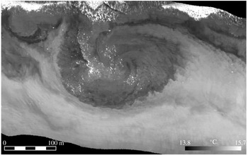
The nearshore littoral zone in the ocean has a unique fluid dynamics. Incident surface gravity waves generated by marine winds offshore break with depth shoaling, and the momentum they lose through breaking is transferred to a substantial degree into wave-averaged alongshore currents and cross-shore sea-level and pressure gradients (often called wave set-up) (Bowen, Inman & Simmons Reference Bowen, Inman and Simmons1968; Longuet-Higgins Reference Longuet-Higgins1970). If there are alongshore bathymetric variations, the alongshore currents can develop stationary recirculation patterns called rip currents. Furthermore, these alongshore and rip currents often exhibit a horizontal-shear instability that leads to a fully developed littoral turbulence comprising transient horizontal-shear waves and horizontally recirculating surf vortices with vertical vorticity (figure 1) (e.g. Oltman-Shay, Howd & Birkemeier Reference Oltman-Shay, Howd and Birkemeier1989; Haller & Dalrymple Reference Haller and Dalrymple2001; Marchesiello et al. Reference Marchesiello, Benshilat, Almar, Uchiyama, McWilliams and Shchepetkin2015). This is often referred to as very-low-frequency (VLF) variability with periods of the order of 10 min. Variations in the incident waves (i.e. waves in groups or with finite alongshore length) provide a further source of transient vertical vorticity that further feeds into the littoral turbulence and vortices (Feddersen Reference Feddersen2014).
Infrared image of surface temperature showing a surf vortex off Huntington Beach, CA (Marmorino, Smith & Miller Reference Marmorino, Smith and Miller2013). The wave swash zone is at the top of the image and deeper water is towards the bottom. The vortex swirl pattern is also evident in an accompanying visible light image, where suspended sand is approximately coincident with the colder temperatures here. The crenellated edges of the swirl pattern are suggestive of an incipient microscopic shear instability, and its amplitude is also seen to amplify in successive images over the next tens of minutes.

There is a substantial literature on surf-zone phenomena and their modelling (n.b. the review in Dalyrimple et al. (Reference Dalyrimple, MacMahan, Reiners and Nelko2011)). With respect to the ‘macroscopic’ currents (i.e. with a scale comparable to the surf-zone width and averaged over the waves), much of the modelling has been performed with wave- and depth-averaged models in two horizontal dimensions (2D), i.e. essentially the shallow-water equations with appropriate parameterizations for the forcing by breaking waves and the damping by bottom-boundary drag, and sometimes with additional conservative wave-averaged dynamical effects (McWilliams, Restrepo & Lane Reference McWilliams, Restrepo and Lane2004). This formulation also excludes the influence of stable density stratification that is often present just outside the breaking zone. Two-dimensional models have seemed satisfactory for many surf phenomena, including many with observational validations. More recently, however, 3D wave-averaged models have begun to be been deployed for the surf zone (Newberger & Allen Reference Newberger and Allen2007; Uchiyama, McWilliams & Shchepetkin Reference Uchiyama, McWilliams and Shchepetkin2010; Kumar et al. Reference Kumar, Voulgaris, Warner and Olabarrieta2012; Marchesiello et al. Reference Marchesiello, Benshilat, Almar, Uchiyama, McWilliams and Shchepetkin2015), with various quantitative differences in their solutions compared with 2D models. In particular, in the regime of wave-driven littoral currents with spontaneously arising surf vortices, the 2D vortices seem to be longer-lived and less deformed than the 3D vortices; i.e. the 2D vortices are more robust (Uchiyama, McWilliams & Akan Reference Uchiyama, McWilliams and Akan2017). There are, of course, also active ‘microscopic’ currents in the surf zone, and they certainly require fully 3D non-hydrostatic models (Kirby & Derakhti Reference Kirby and Derakhti2018).
The purpose of this paper is to test nearshore vortex robustness in 2D and 3D, as well as in 3D with density stratification. For simplicity and a focus on the vortex behaviour by itself, wave effects are not included here. While this idealized problem is only one aspect of the surf-zone phenomena described above, it is relevant both to the nearshore dispersion of material concentrations (deemed to be dominated by the horizontal vortical flows in Spydell & Feddersen (Reference Spydell and Feddersen2009)) and to the question of which aspects of the surf-zone and inner-shelf (lying outside the wave-breaking zone) dynamics are well characterized with a depth-averaged model and which require a fully 3D model.
The model is the hydrostatic Regional Oceanic Modeling System (ROMS; Shchepetkin & McWilliams Reference Shchepetkin, McWilliams, Temam and Tribia2009; Uchiyama et al. Reference Uchiyama, McWilliams and Shchepetkin2010), which is generally usable for realistic simulations of macroscopic shelf and surf currents under the influences of many contributing processes. The idealized problem has an initial pair of opposite-signed vortices (i.e. a dipole) located in shallow water on a uniformly sloping beach and oriented so that their mutual advective tendency induces propagation into deeper water. The resulting depth change in turn induces change in their strength and shape, and thus provides a mildly disruptive perturbation (mimicking, e.g., the disruption of surf vortices in littoral turbulence). The robustness question is how the dipole responds to this perturbation. To isolate the essential dynamics, no incident surface gravity wave interaction effects are included here, apart from the long hydrostatic (i.e. shallow-water) gravity waves associated with the variable free surface coupled to the depth-averaged currents in the ROMS. Thus, the problem here is more precisely posed as vortices in the inner shelf (i.e. without waves), and as such is both incomplete with respect to surf vortices and more generally relevant to inner-shelf vortices generated by other processes. Dipole vortices have been extensively studied in other contexts (some cited in § 3), although as yet without the combination of slope and stratification. Our interest is not in dipole vortices per se, but as a means of illustrating the robustness question.
2 Problem posing
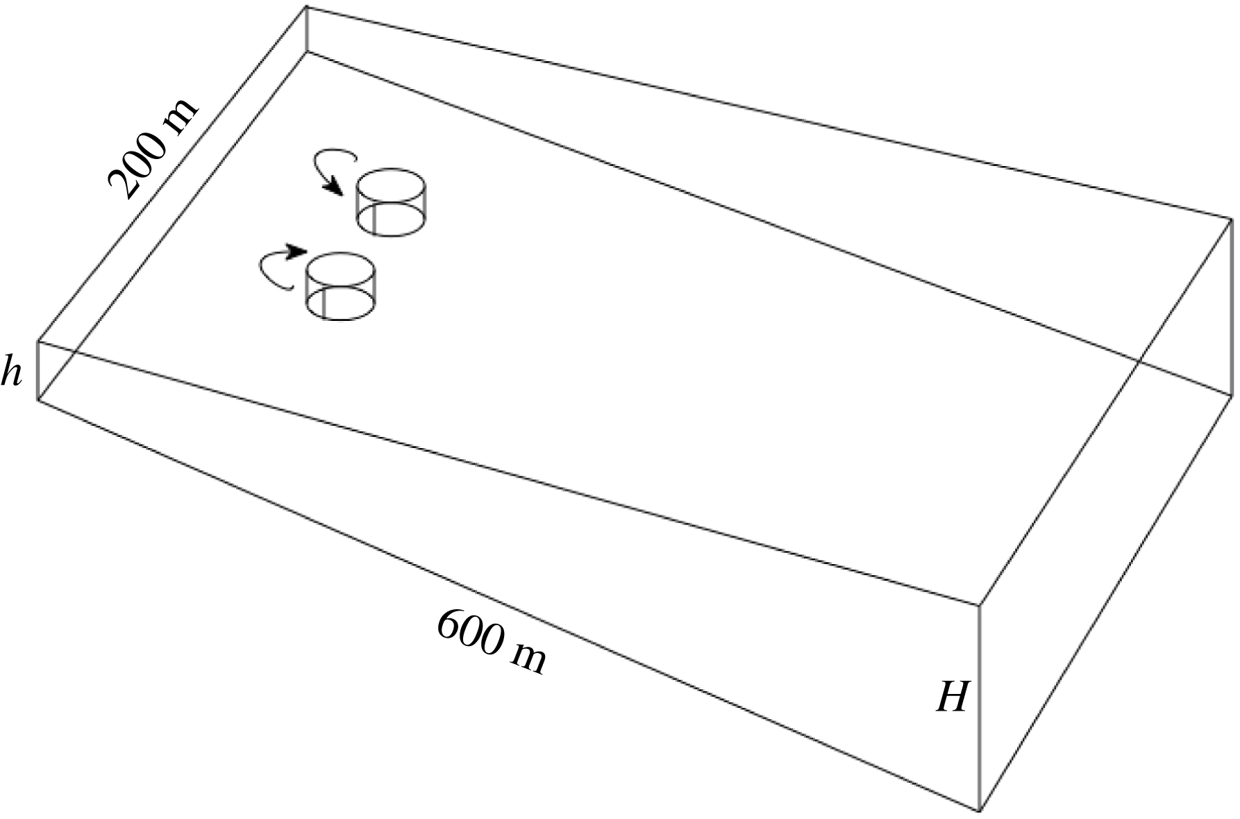
The geometry of the initial conditions and domain is sketched in figure 2. Here,
 $h$
is the inshore minimum depth, which we choose to be 0.25 m;
 $H$
is a variable outer depth that controls the steepness of the bottom slope; we have obtained a set of solutions with
 $H=5$
, 10 and 20 m at an offshore distance of
 $L_{x}=$
600 m. The alongshore width is
 $L_{y}=$
200 m. For each
 $H$
, a set of three alternative model solutions is obtained: shallow water (case 2DU, with the U denoting unstratified), 3D with no density stratification (case 3DU) and 3D with a linear density stratification (case 3DS). For the 3DS case, the surface temperature
 $T=21\,^{\circ }\text{C}$
and the bottom temperature
 $T=20.4\,^{\circ }\text{C}$
at
 $x=L_{x}$
; e.g. the value of the buoyancy frequency is
 $N=\sqrt{\unicode[STIX]{x1D6FC}g\unicode[STIX]{x2202}_{z}T}=1.8\times 10^{-2}~\text{s}^{-1}$
when
 $H=10$
m (
 $\unicode[STIX]{x1D6FC}=2\times 10^{-4}~\text{C}^{-1}$
is the thermal expansion coefficient for sea water).
Sketch of the initial configuration for a barotropic vortex dipole aimed offshore in shallow water over a uniformly sloping bathymetry. Here,
 $h=0.25$
m and
 $H$
are the resting depths at cross-shore locations of
 $x=0$
and 600 m.
 $\text{(Offshore, alongshore)}=(x,y)=\text{(east, north)}$
coordinates respectively.

All solutions start with the same initial condition for the flow, i.e. a pair of barotropic vortices (figure 2). Their currents are independent of depth, and hence consistent with an initial 2D flow. Their vorticity centres are located at
 $x=100$
m offshore and mutually separated by
 $\unicode[STIX]{x0394}y=$
10 m in the alongshore centre of the domain. The initial vertical vorticity field is a superposition of individual axisymmetric monopoles of opposite sign,
 $$\begin{eqnarray}\unicode[STIX]{x1D701}^{z}(r)=\frac{\unicode[STIX]{x1D701}_{0}}{(1+(r/r_{0})^{2})^{2}},\end{eqnarray}$$
with amplitude
 $\unicode[STIX]{x1D701}_{0}=\pm 0.9\times 10^{-2}~\text{s}^{-1}$
and radial size
 $r_{0}=10$
m. The coordinate
 $r=\sqrt{(x-x_{c})^{2}+(y-y_{c})^{2}}$
is the radial distance from the vortex centre located at
 $(x_{c},y_{c})$
. The accompanying azimuthal velocity profile
 $V(r)$
and surface elevation
 $\unicode[STIX]{x1D702}(r)$
(as determined by cyclostrophic balance) are
 $$\begin{eqnarray}\displaystyle \left.\begin{array}{@{}c@{}}\displaystyle \unicode[STIX]{x1D701}^{z}=\frac{1}{r}\unicode[STIX]{x2202}_{r}[rV]\quad \Rightarrow \quad V(r)=\frac{v_{0}r_{0}}{r(1+(r/r_{0})^{2})},\quad v_{0}=\frac{r_{0}\unicode[STIX]{x1D701}_{0}}{2},\\ \displaystyle -g\unicode[STIX]{x2202}_{r}\unicode[STIX]{x1D702}=-\frac{V^{2}}{r}\quad \Rightarrow \quad \unicode[STIX]{x1D702}(r)=\frac{\unicode[STIX]{x1D702}_{0}}{1+(r/r_{0})^{2}},\quad \unicode[STIX]{x1D702}_{0}=-\frac{r_{0}^{2}\unicode[STIX]{x1D701}_{0}^{2}}{8g}.\end{array}\right\} & & \displaystyle\end{eqnarray}$$
From the preceding values for
 $\unicode[STIX]{x1D701}_{0}$
and
 $r_{0}$
, accompanying values here are a swirl velocity
 $v_{0}=0.05~\text{m}~\text{s}^{-1}$
and a surface elevation
 $\unicode[STIX]{x1D702}_{0}=10^{-4}$
m. Both are somewhat weaker than is likely to be true for the situation in figure 1, but we would expect an approximate invariance of the advectively controlled behaviour with proportionally increased
 $\unicode[STIX]{x1D701}_{0}$
and evolutionary rate, and have confirmed this expectation with a modest survey of solutions with different
 $r_{0}$
and
 $\unicode[STIX]{x1D701}_{0}$
values. Such a monopole vortex by itself is an inviscid stationary state over a flat bottom, and it is linearly stable with respect to 2D horizontal-shear instability because it has no inflection point.
The nearby superposition of these two vortices is not necessarily a stable configuration, although our solutions in § 3 do not show any obvious patterns of 2D shear instability. The vortex with positive
 $\unicode[STIX]{x1D701}_{0}$
– by convention called cyclonic because it has the same sign as the Coriolis frequency
 $f=10^{-4}~\text{s}^{-1}$
– is located to the north (
 $y_{c}>0$
) of the negative (anticyclonic) vortex (see the arrows in figure 2). This orientation gives the dipole an
 $x$
propagation tendency in the eastward offshore direction towards deeper water, with a behaviour similar to the uniformly propagating strictly 2D dipole solution in (Lamb Reference Lamb1932, § 155). The choice of the monopole profiles in (2.1)–(2.2) is somewhat arbitrary, and no special care is taken in modifying their shape in forming the dipole (n.b., in Lamb’s dipole there is an elongation of the vorticity isolines perpendicular to the centre separation line). As a consequence, there is an early evolutionary period of cyclostrophic adjustment, as the two monopoles slightly modify their
 $\unicode[STIX]{x1D701}^{z}$
and
 $\unicode[STIX]{x1D702}$
shapes into a more slowly evolving propagating dipole vortex. During this early period, shallow-water gravity waves are radiated away from the adjusting vortex.
Conservation of potential vorticity in its rotating shallow-water approximation is
 $$\begin{eqnarray}\frac{\text{D}q_{sw}}{\text{D}t}\approx 0,\quad q_{sw}=\frac{f+\unicode[STIX]{x1D701}^{z}}{h+\unicode[STIX]{x1D702}}\approx \frac{\unicode[STIX]{x1D701}^{z}}{h}.\end{eqnarray}$$
This implies that as the dipole moves into deeper water (larger
 $h$
), carrying some of its core fluid with it, the vorticity in the dipole centres will increase in magnitude (Arthur Reference Arthur1962). In the 2DU cases, we can anticipate that this will be a prominent effect, but it is not known a priori how much this behaviour will carry over into the 3DU and 3DS cases.
The problem posing is completed with
 $f=10^{-4}~\text{s}^{-1}$
(i.e. small compared with the peak vorticity), K-profile parameterization for the vertical eddy diffusion, a drag coefficient of
 $C_{D}=3\times 10^{-3}$
used in a quadratic bottom stress law, and weak lateral diffusion as part of the upstream-biased advection operator in the ROMS (Shchepetkin & McWilliams Reference Shchepetkin, McWilliams, Temam and Tribia2009). None of these influences have an especially large effect over the multihour period of model integration, but the bottom drag influence is evident in the weak decay of the
 $\unicode[STIX]{x1D701}^{z}$
extrema and the volume-integrated energy.
With respect to the numerical discretization, the horizontal grid size is
 $\text{d}x=\text{d}y=1$
m, the number of vertical sigma levels is
 $N=20$
for the 3D solutions, uniformly distributed in depth, and the barotropic-mode time-step size is
 $\text{d}t=0.05$
s, consistent with resolving shallow-water gravity waves where the phase speed
 ${\approx}\sqrt{gh}$
is largest. Solution behaviours are not sensitive to further refinements of these discretization values.
3 Results
To establish a reference standard, we first consider the set of three alternative model cases for the dipole vortex over a flat bottom, which for definiteness we take as having a uniform depth of 10 m. In an integration over a period of 4 h, the dipole propagates almost directly offshore at an average speed of approximately
 $0.01~\text{m}~\text{s}^{-1}$
. Over this period, the loss of volume-integrated kinetic energy
 $KE$
in (3.1) is approximately 5 % of the initial value and the decrease in the peak magnitude of
 $\unicode[STIX]{x1D701}^{z}$
at the surface is approximately 14 % (in contrast to the prediction of no change from (2.3)), in association with minor changes in its pattern shape and bottom drag. These quantitative statements apply equally to each of cases 2DU, 3DU and 3DS. Thus, in the absence of disruption (e.g. by depth change), they all exhibit a weakly decaying approximation to a uniformly propagating barotropic dipole vortex over a flat bottom.
 $$\begin{eqnarray}KE(t)={\textstyle \frac{1}{2}}\iiint \boldsymbol{u}^{2}\,\text{d}x\,\text{d}y\,\text{d}z,\quad Ens(t)=\iiint |\unicode[STIX]{x1D735}\times \boldsymbol{u}|^{2}\,\text{d}x\,\text{d}y\,\text{d}z.\end{eqnarray}$$
The cases of more interest are those with a sloping bottom because of the disruption this provides to the propagating dipole vortex (Centurioni Reference Centurioni2002). Our standard integration period is
 $t_{max}=4$
h, which is sufficient to establish the differences in behaviour among the three dynamical models. We made a complete set of dynamical cases for both the uniform-depth case described in the previous paragraph and the three different slope values with
 $H=5$
, 10 and 20 m at
 $x=L_{x}$
(figure 2). From these, we conclude that the qualitative differences among the different dynamical cases over a sloping bottom are essentially similar for all values of
 $H$
. Therefore, for the most part, we will report only on the
 $H=10$
m solutions.
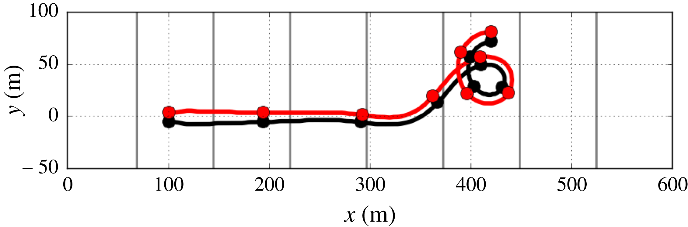
However, to first illustrate the grossest aspect of the depth-induced disruption, namely the change in vortex strength as argued in (2.3) and its consequence on the dipole propagation, we show a long-time (16 h) trajectory for the case 2DU vortex as it moves offshore over the case with the steepest slope, i.e.
 $H=20$
m (figure 3). The initial adjustment causes a modest reshaping of the vortex, with the centres increasing their separation distance while propagating offshore. The vorticity extrema increase in magnitude over the first
 $10^{4}$
s, as anticipated in (2.3), during which the centres move closer together. After this period, however, there is an oscillatory ‘instability’ in the trajectory that causes the dipole vortex to meander in its trajectory over a longer period. It can be understood by a point-vortex argument based on (2.3). If a small perturbation causes one centre to become stronger (here the cyclone), it will tend to advect the weaker centre (anticyclone) around it (in an anticlockwise direction) by pushing it into deeper water, where the weaker centre will then strengthen, and the vortex will come back into a more equal balance of mutual advection along a straight trajectory oriented now in a different direction that is no longer perpendicular to the slope. With the previously weaker anticyclonic centre now leading on the deeper-water side, it will in turn strengthen and pull the cyclonic centre in the clockwise direction, thus strengthening it, etc., with the long-time outcome becoming an oscillatory and wandering trajectory. While all this meandering is going on, the disrupted vortices begin to weaken, with decreasing peak vorticity amplitudes after their early maximum around
 $t=10^{4}$
s, and they are reduced to approximately half of the initial amplitude in
 $|\unicode[STIX]{x1D701}^{z}|$
by the end time of
 $t=5.8\times 10^{4}$
s. With respect to the integral variance measures (3.1), the meandering dipole also exhibits a monotonically decreasing kinetic energy
 $KE$
(down to approximately 43 % by the end time) as well as a first increasing and then decreasing enstrophy
 $Ens$
(down to 55 % by the end). These changes are much greater than in the flat-bottom cases over an equivalent integration time, for case 2DU in particular. Of course, in these 2DU cases, because
 $\unicode[STIX]{x1D735}$
is purely horizontal and
 $w$
is nearly zero (in association with the small
 $\unicode[STIX]{x1D702}$
changes),
 $Ens$
measures only the variance of the vertical vorticity
 $\unicode[STIX]{x1D701}^{z}=\hat{\boldsymbol{z}}\boldsymbol{\cdot }\unicode[STIX]{x1D735}\times \boldsymbol{u}$
. Thus, although the dipole vortex is substantially disrupted as its traverses the sloping bottom, it retains its general dipole shape and propagation behaviour, although the expectation of bulk
 $q_{sw}$
conservation (2.3) does not hold. Similar behaviour occurs for the other 2DU cases with their different
 $H$
values (i.e. different slopes).
Trajectory of the maximum (red) and minimum (black) in surface vorticity
 $\unicode[STIX]{x1D701}^{z}(x,y,0,t)$
for the 2DU case with
 $H=20$
m over an integration period of 16 h, with dots at 2 h intervals. Grey contours indicate isobaths with an interval of
 $\text{d}h=2.5$
m.

Now, we return to our primary experiments: a comparison of the different dynamical cases for
 $H=10$
over the shorter integration period of
 $t_{max}=1.44\times 10^{4}~\text{s}=4$
h, which is long enough to demonstrate differences among the cases. They all exhibit the gross behaviour of offshore propagation of the dipole with relatively little meandering during this shorter period, but they differ considerably in their pattern evolutions.
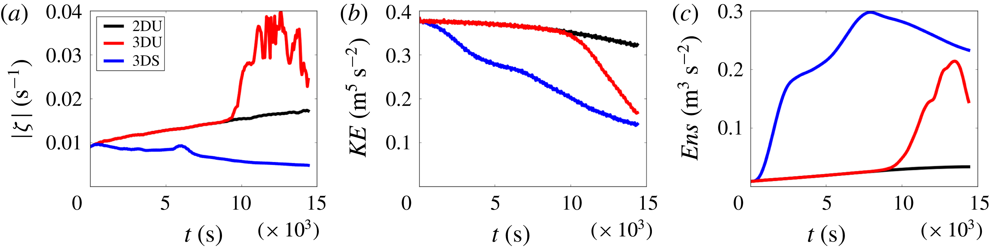
Time series for the three different dynamical cases with
 $H=10$
m over a period of 4 h: surface vorticity magnitude
 $\max |\unicode[STIX]{x1D701}^{z}(x,y,0)|$
(a),
 $KE$
(b) and
 $Ens$
(c). The line colours for the cases are indicated in the inset in (a).

Starting with time series, the different model solutions are compared in figure 4. The barotropic solution in case 2DU shows a monotonic increase in the peak vorticity at the surface, as anticipated with potential vorticity conservation (2.3). Similarly, its total enstrophy
 $Ens(t)$
increases monotonically, due almost entirely to the vertical component,
 $\unicode[STIX]{x1D701}^{z2}$
, because there are no vertical derivatives in this model and the
 $w$
associated with surface elevation changes is small; hence, the horizontal component of
 $Ens$
is small. (All of the solutions exhibit propagating shallow-water gravity waves throughout their integrations, especially during the initial adjustment phase, but they are quite weak compared with the vortex currents.) The kinetic energy
 $KE(t)$
decays monotonically due to lateral diffusion and bottom drag. Its change over 4 h is a decrease by 17 %, which is only a modest amount but still is much larger than the comparable case over a flat bottom (i.e. 5 %, as stated above), indicating the disruptive effect of the changing water depth as the vortex propagates offshore.
The unstratified case 3DU solution starts by following the evolutionary path of the case 2DU solution. However, at a time of around 2.5 h (
 $10^{4}$
s), it shows an explosive growth in the peak amplitude of the surface
 $\unicode[STIX]{x1D701}^{z}$
and in
 $Ens(t)$
. For the latter, it is the horizontal vorticity components,
 $(\unicode[STIX]{x1D701}^{x},\unicode[STIX]{x1D701}^{y})\approx (-\unicode[STIX]{x2202}_{z}v,\unicode[STIX]{x2202}_{z}u)$
, that cause the largest enstrophy growth, with the vertical component
 $\unicode[STIX]{x1D701}^{z}$
enhanced over its case 2DU value only by approximately a factor of 2. When this explosion occurs, the
 $KE(t)$
decreases rapidly, indicating an enhanced dissipation by a cascade of energy down to smaller scales. While we cannot give a precise explanation of this apparent vortex instability that amplifies into subvortex-scale turbulence, we heuristically see it as consistent with the instability of an elliptically deformed monopole vortex that in its axisymmetric state is linearly stable (e.g. Pierrehumbert Reference Pierrehumbert1986). The adjacent dipole vorticity centres induce such an elliptical deformation on one another, in addition to whatever other asymmetric flow patterns may arise. This instability grows most rapidly for perturbations with the smallest inviscid scales, consistent with the small-scale patterns that are shown in figure 6. Even in the 3DU case with a flat bottom, discussed at the start of the section, there is a discernible departure of
 $Ens(t)$
from its decreasing vertical component around the same time of 2.5 h, leading to a net increase in
 $Ens$
of approximately 6 % over the 4 h integration period, indicating the milder onset of a similar instability even in that case (but much less than the increase in
 $Ens$
that occurs over a slope). In other studies of unstratified dipole vortices over a flat bottom, similar 3D breakdowns are sometimes seen (Duran-Matute et al.
Reference Duran-Matute, Albagnac, Kamp and van Heijst2010; van Heijst Reference van Heijst2014).
Another perspective is that vortex stretching and tilting (i.e.
 $[(\unicode[STIX]{x1D735}\times \boldsymbol{u})\boldsymbol{\cdot }\unicode[STIX]{x1D735}]\boldsymbol{u}$
) are enabled in the 3D vorticity equation but absent in 2D; their occurrence is demonstrated by the
 $Ens$
explosion in figure 4 and their rates are explicitly diagnosed in Uchiyama et al. (Reference Uchiyama, McWilliams and Akan2017). This process allows 3D vorticity perturbations to amplify even as transient growth, if not literally as an instability (Trefethan et al.
Reference Trefethan, Trefethan, Reddy and Driscoll1993). In the 3DU case, this amplification is unimpeded by the gravitational force, whereas in the 3DS case, it is modified by the stable density stratification, as discussed next.
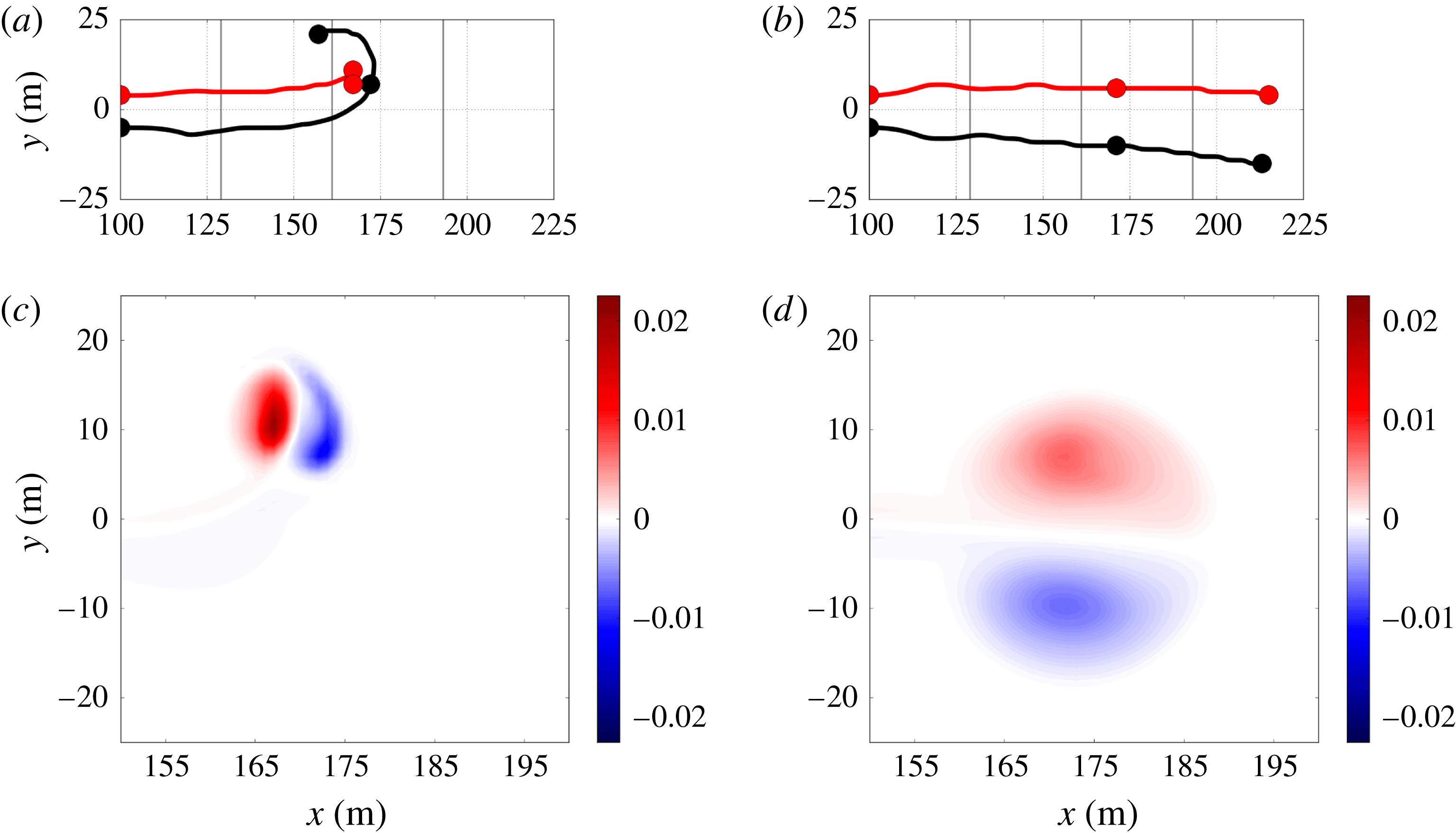
(a,b) Four hour trajectories for the horizontal maximum (red) and minimum (black) vorticity centres for case 3DS, with dots every two hours, and (c,d)
 $\unicode[STIX]{x1D701}^{z}(x,y,z_{0},t_{0})$
at the middle time,
 $t_{0}=7200~\text{s}=2$
h. Panels (a,c) are at the bottom (
 $z_{0}=-h(x)$
) and (b,d) are at the surface (
 $z_{0}=0$
). Here,
 $H=10$
m and the grey contours in (a,b) are isobaths with
 $\text{d}h=2.5$
m.

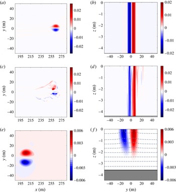
Cross-sections of
 $\unicode[STIX]{x1D701}^{z}$
(
 $\text{s}^{-1}$
) for the three cases with
 $H=10$
m at the time
 $t=1.23\times 10^{4}~\text{s}=3.4$
h: case 2DU (a,b), case 3DU (c,d) and case 3DS (e,f). Panels (a,c,e) are for a horizontal section,
 $\unicode[STIX]{x1D701}^{z}(x,y,0)$
. Panels (b,d,f) are for a vertical section
 $\unicode[STIX]{x1D701}^{z}(x_{0},y,z)$
at the offshore location
 $x_{0}$
that passes through the surface vorticity cyclonic extremum at this time:
 $x_{0}=262$
m (2DU), 257 m (3DU) and 205 m (3DS). In the vertical section, the local bottom depth
 $D(x_{0})$
is indicated by a dark horizontal line at
 $z=-D$
with shading below it. One should notice the different colourbar ranges for the different cases. In the cross-section for case 3DS (f), the isotherms are the dashed-grey lines with
 $\text{d}T=0.03\,^{\circ }\text{C}$
; it should be recalled that cases 2DU and 3DU are isothermal.

The stratified case 3DS solution behaves quite differently from either case 2DU or 3DU. From the outset, its surface vorticity maximum does not increase as anticipated from shallow-water
 $q_{sw}$
conservation (2.3) even as it moves offshore into deeper water; its
 $KE(t)$
more rapidly decreases and its
 $Ens(t)$
rapidly increases due to increasing vertical shear of
 $\boldsymbol{u}$
, hence increasing the variance of its horizontal vorticity components. Furthermore, a topological transformation in the dipole vortex occurs starting at around
 $t=5\times 10^{3}~\text{s}=1.5$
h: in the lower-half of the water column, the cyclonic vorticity centre strengthens with an increased depression in its mid-depth isothermal surfaces, implying an amplified central hydrostatic pressure in cyclostrophic balance, while the isothermal surfaces lift over the anticyclone, implying a weaker vortical flow in cyclostrophic balance. This causes an anticlockwise turning of the deeper vortex pair towards the northeast, and the stronger cyclone pulls the weaker anticyclone around it in an anticlockwise direction and deforms its shape while remaining nearly stationary in space and circular in shape over the rest of the integration period (figure 5). Meanwhile, near the surface, the vorticity centres remain approximately equal in strength and continue to propagate eastward in cyclostrophic balance with their surface elevation depressions. These divergent trajectories between the upper and lower parts of the dipole act to split the vortex vertically. The asymmetric deeper pair of vorticity centres evolves into a weak stationary cyclonic monopole, while the more symmetric upper pair persists as a coherent vortex. In the time series, the spitting event is marked by a temporary increase in the
 $\unicode[STIX]{x1D701}^{z}(x,y,0)$
extremum and by diminished rates of
 $KE(t)$
decay and
 $Ens(t)$
growth. In the late stages, after
 $Ens(t)$
peaks at around
 $t=8\times 10^{3}~\text{s}=2.3$
h, there is steady decay of the surface extremum,
 $KE$
and
 $Ens$
. In this later period, the dipole is surface intensified and is no longer importantly influenced by the sloping bottom as it propagates further offshore while approximately conserving its 3D Ertel potential vorticity,
 $q_{E}=(f\hat{\boldsymbol{z}}+\unicode[STIX]{x1D735}\times \boldsymbol{u})\times \unicode[STIX]{x1D735}T$
. This late-time propagation behaviour is similar to that of a stratified dipole over a flat bottom (Voropayev, Fernando & Morrison Reference Voropayev, Fernando and Morrison2008).
The flow structures during the late stage of these model integrations (
 $t=1.23\times 10^{4}~\text{s}=3.42$
h) are illustrated in figure 6 with horizontal and vertical sections of
 $\unicode[STIX]{x1D701}^{z}$
. The barotropic vortex in case 2DU is propagating eastward with strong symmetry between the vorticity centres, and they are independent of depth (by construction). The centres are close together and their pattern is elongated in the propagation direction, much like in Lamb’s dipole solution. Among the three cases, it is the most coherent and it has propagated the farthest to the east. The 3D unstratified barotropic vortex in case 3DU has propagated almost as far, but it exhibits fragmentation in both its horizontal and vertical patterns. Nevertheless, in some coarse-grained sense, it still behaves like an almost barotropic dipole vortex, at least over this 4 h integration period. Finally, the stratified dipole vortex in case 3DS, after the vertical splitting event described above, has recovered a very coherent pattern, but its vertically connected extent is restricted to the upper-half of the water column. In case 3DS, it has a larger horizontal size, a wider separation of its vorticity centres, a weaker vorticity amplitude and thus a slower eastward propagation speed compared with the barotropic dipole in case 2DU. Its thermal structure is a cold anomaly with respect to its surroundings that weakens with depth. This is consistent with cyclostrophic and hydrostatic balance for a surface-intensified vortex: the sea-level depression at the vortex cores (
 $\unicode[STIX]{x1D702}<0$
) has a low-pressure anomaly that weakens with depth (
 $\unicode[STIX]{x1D70C}_{0}^{-1}\unicode[STIX]{x2202}_{z}p<0$
), hence a negative thermal anomaly in the upper levels (
 $T=-(\unicode[STIX]{x1D70C}/\unicode[STIX]{x1D6FC}\unicode[STIX]{x1D70C}_{0})<0$
, with
 $\unicode[STIX]{x1D6FC}$
the thermal expansion coefficient), hence an uplift of the isotherms, as seen in figure 6(f).
4 Summary and discussion
Depth-averaged fluid dynamics are very useful in understanding many aspects of nearshore currents. These include the formation of alongshore and rip currents when waves break and the occurrence of current instabilities that give rise to shear waves and vortices in surf turbulence. However, we have shown here with an idealized dipole vortex over a sloping bottom that the 2D depiction of coherent surf vortices is incomplete and inaccurate in comparison with a 3D model. In particular, the vortex robustness is overestimated in 2D, as previously noted in more complex flow simulations (Uchiyama et al. Reference Uchiyama, McWilliams and Akan2017).
This experimental result adds impetus to the evolution of nearshore modelling towards including fully 3D dynamics. In the surf zone itself, when the density is nearly uniform due to mixing by breaking waves, the unstratified 3D model (case 3DU) indicates a moderate degree of fragility of its barotropic vortices to elliptical instability and to vortex stretching and tilting. For surf vortices that move offshore into stratified water, there can be an emergence of surface-intensified vortices, after a somewhat dissipative transition, that then achieve a degree of coherence in their further lifetime while somewhat insulated from further depth changes.
A question arises: how well can the hydrostatic model used here represent the true fluid dynamics of surf vortices? Depth-averaged models are inherently hydrostatic and, as noted, have been found to be useful for many surf phenomena, including vortex emergence (figure 1). It is likely that much of the 3D flow structure on microscopic scales smaller than the macroscopic vortices will be partly non-hydrostatic, namely the 3D vortex instability in case 3DU and much of the vortex tilting and stretching behaviours; a non-hydrostatic model would be needed to follow these processes in detail. With respect to the macroscopic behaviours of vortex propagation, decay, incipient horizontal enstrophy generation and, in case 3DS, structural transformation, we are confident that the hydrostatic approximation is adequate. A definitive demonstration of this assertion could only be made with a non-hydrostatic model, but in lieu a consistency test has been made by comparing the magnitude of
 $\unicode[STIX]{x2202}_{t}w$
with the anomalous vertical pressure gradient,
 $\unicode[STIX]{x1D70C}_{0}^{-1}\unicode[STIX]{x2202}_{z}p$
, at a middle depth level in the midst of the most violent macroscopic event in case 3DS, namely its vertical fissioning around
 $t=2$
h (figure 5). The magnitude of
 $\unicode[STIX]{x2202}_{t}w$
is nearly three orders of magnitude smaller than the vertical pressure gradient anomaly; i.e. the macroscopic behaviour is quite safely hydrostatic.
A modern scientific frontier is the combined interactions among surface gravity waves, turbulent nearshore currents and turbulent submesoscale currents in the deeper stably stratified water over the continental shelf (Dauhajre, McWilliams & Uchiyama Reference Dauhajre, McWilliams and Uchiyama2017). In all of these combinations, the dynamics are often 3D with important effects from stratification and, at least for shelf currents, from the Earth’s rotation (Lentz & Fewings Reference Lentz and Fewings2012; Kumar & Feddersen Reference Kumar and Feddersen2017).
Acknowledgements
We appreciate technical assistance by D. Dauhajre. This research is supported by the US Office of Naval Research (grant N00014-15-1-2645), the National Science Foundation (grant OCE-1355970) and Japan Society for the Promotion of Science, Grants-in-Aid for Scientific Research, grant numbers 15KK0207 and 15H04049. This work used the Extreme Science and Engineering Discovery Environment (XSEDE), which is supported by National Science Foundation grant number ACI-1548562.