Introduction
The volatility of milk prices is a challenge for dairy farmers leading to financial struggles, as proved once again by the milk crisis in 2016. Consequently, in order to operate efficiently, dairy farmers have to focus on optimizing their production factors. International studies have revealed a direct or indirect causal relationship between specific production parameters and efficiency parameters. Stankov et al. (Reference Stankov, Stoyanova and Petrov2015) detected a positive correlation between milk yield and profit (r = 0.72) and between farm size and profit (r = 0.72). In previous efficiency studies (MacDonald et al., Reference MacDonald, O'Donoghue, McBride, Nehring, Sandretto and Mosheim2007), with increasing herd size, the total costs of production fell and the net return rose, while the largest farms had the lowest total feeding costs. Thus, for dairy production, economies of scale seem to play an important role, meaning that for farmers who produce efficiently, costs decline as output expands (Mathijs and Swinnen, Reference Mathijs and Swinnen2001; Steinfeld et al., Reference Steinfeld, Wassenaar and Jutzi2006; MacDonald et al., Reference MacDonald, O'Donoghue, McBride, Nehring, Sandretto and Mosheim2007). Furthermore, reproductive efficiency also affects dairy farm profitability (De Vries, Reference De Vries2006). This is because cows in well-managed herds have longer productive lifetimes. Also, in herds with higher reproduction rates, fewer replacement animals are needed (Knapp et al., Reference Knapp, Laur, Vadas, Weiss and Tricarico2014). According to Groenendaal et al. (Reference Groenendaal, Galligan and Mulder2004) and De Vries (Reference De Vries2006), a reduction in days open beyond the optimum could also improve dairy profitability. Not only does fertility itself play an important role in dairy farming profitability but problems concerning fertility very often occur due to the health problems of individual cows or the whole dairy herd. Disease results in high costs for farms, not only because of the costs of vets and medication but also due to loss of performance. In the studies of Kvapilik et al. (Reference Kvapilik, Hanuš, Bartoň, Klimešová and Roubal2015), mastitis was responsible for a 14% increase in medication and curing costs and for 53% lower revenues from milk sales compared with healthy cows. For lame cows, test-day and peak lactation milk yield decreased by 2 kg/day/cow (Mitev et al., Reference Mitev, Gergovska, Miteva and Penev2011). From the efficiency point of view, decreasing mortality and morbidity rates are decisive for dairy farmers, because animals which die or have to be culled before their first lactation use a significant amount of energy and resources (e.g. feed and work) without producing marketable food. Furthermore, half of the overall costs of a milk production system are feed costs (Moran, Reference Moran and Moran2005). In this case, not only does cost efficiency plays a role but also resource efficiency, i.e., using the lowest number of inputs to create the greatest number of outputs (Lagomasino et al., Reference Lagomasino, Zatzick and Chambers2010). In dairy farming, herd management is the key factor which determines resource efficiency. The role of herd management is particularly important in intensive farming systems. Approximately 45–50% of the increase in milk yields under intensive management has been achieved through improvements in management practices (Hansen, Reference Hansen2000; VanRaden, Reference VanRaden2004; Shook, Reference Shook2006). Herd management observes and evaluates a complex set of parameters that influence each other, including fertility, health, feeding and performance. Therefore, a method is required to model the relationships between the afore-mentioned variables, taking into account the multi-dimensional nature of the interactions.
Regression analysis is a common tool to conduct efficiency studies, but this method only investigates unilateral relations (Klarmann, Reference Klarmann2008). Partial least squares structural equation modelling (PLS-SEM), first generated by Wright (Reference Wright1921), enables an estimation of parameters which are not themselves measurable, the so-called latent variables (Hair et al., Reference Hair, Hult, Ringle and Sarstedt2014). Structural equation modelling (SEM) has increased in popularity for multigroup analysis, not only in agriculture (Lamb et al., Reference Lamb, Shirtliffe and May2011; Valente et al., Reference Valente, Rosa, Gianola, Wu and Weigel2013) but also in milk production (de los Campos et al., Reference de los Campos, Gianola and Heringstad2006; Heringstad et al., Reference Heringstad, Wu and Gianola2009). Thus, in the current study, SEM was investigated as an alternative method for the estimation of complex interactions between the latent variables relating to herd management in milk production. Moreover, interactions were investigated between the variables determining efficiency (cause variables) as well as the role of these cause variables in increasing this efficiency.
Materials and methods
Data origin and data structure
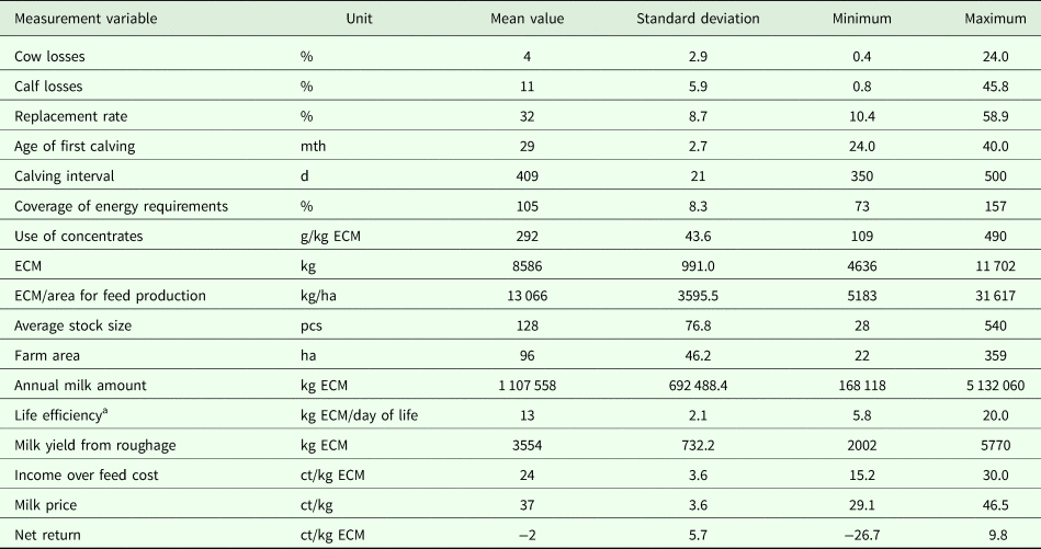
The data for the current study originate from the cattle advisory board of the ‘Chamber of Agriculture Schleswig-Holstein’ and are based on the annual branch settlements of individual farms. The data set contains structural parameters (e.g. average stock size, farm area) and economic parameters (e.g. labour costs, feed costs, net return). Information on biological performance (e.g. milk yield, age of first calving, replacement rate) is also included. The current study was based on data from a total of 943 branch settlements of dairy farms in Schleswig-Holstein (Northern Germany): 480 data sets originated from the marketing year 2012 and 463 from 2013. To avoid breed-related influences on the performance, only farms keeping German Holstein cattle were included in the study. Table 1 shows the structure of the data set. The farms had an average stock size of 128 cows, with a range between 28 and 540 cows per farm. The area for feed production was 96 ha on average, ranging from 22 to 359 ha. The farms had an energy-corrected milk yield (ECM) ranging from 4636 to 11 702 kg/cow/year and between 2002 and 5770 kg milk yield from roughage/cow/year. Net return, which is used as a measure of economic efficiency in the SEM, ranged from −26.7 to 9.8 ct/kg ECM. The values for life efficiency, which are used as a measure of biological efficiency, ranged from 5.8 to 20.0 kg ECM/day of life.
Descriptive statistics of the data set (the measurement variables are average values of the farms)
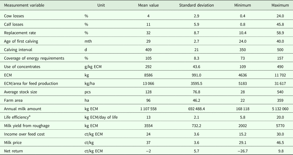
ECM, energy-corrected milk yield.
a Life efficiency (LE) = milk yield per day of life, calculated as: LE = lifetime performance/(age of first calving + productive lifetime).
General scheme of a structural equation model
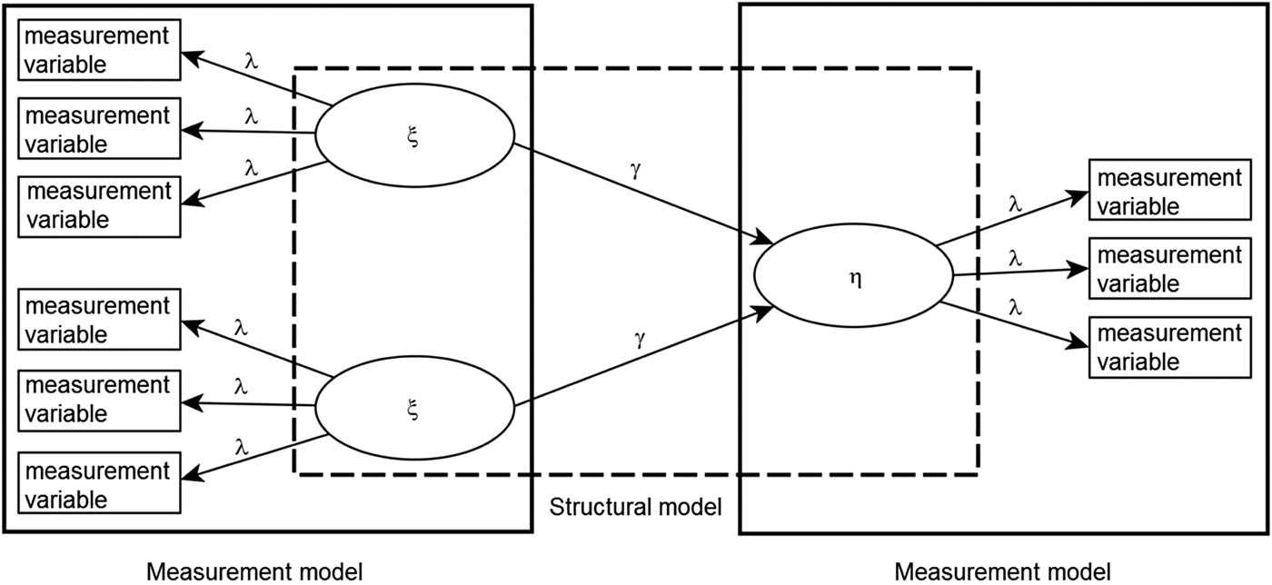
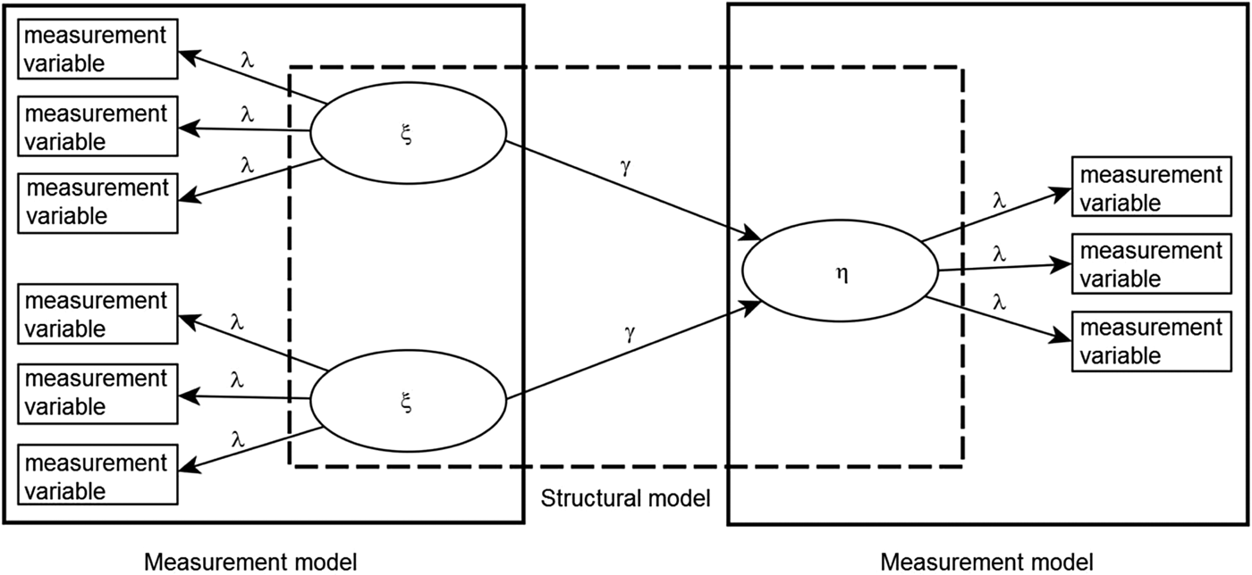
An SEM is a construct of different types of variables, which illustrates and calculates relationships between them. It distinguishes between latent variables, which are not themselves measurable, and measurement variables, which enable an estimation of the latent variables. An SEM consists of two parts: the structural model and at least two measurement models (Fig. 1). A measurement model consists of a set of measurement variables which together characterize a latent variable respectively. The structural model represents the relationships between the latent variables (ξ, η), which are characterized as arrows connecting each other (path coefficients, γ). There is a distinction between two types of latent variables: latent cause variables and latent effect variables. Thus, in an SEM, a set of cause variables influences one or more effect variables. The latter are within the scope of the current study. Also, cause variables have to be distinguished into endogenous (dependent) and exogenous (independent) cause variables. This implies that endogenous cause variables are also influenced by other latent variables, whereas exogenous variables are not influenced by other latent variables. Therefore, the coefficient of determination (R 2) is only calculated for endogenous but not for exogenous variables.
Scheme of a simplified structural equation model (modified after Nitzl, Reference Nitzl2010). Circles represent latent variables (ξ, η), rectangles represent measurement variables. Arrows between circles represent relationships between latent variables (path coefficients, γ). Arrows between circles and rectangles represent indicator reliabilities (of the respective measurement variables, λ). See Fig. 2 for a detailed description of the structural equation model in this study and further explanations of the investigated relationships.
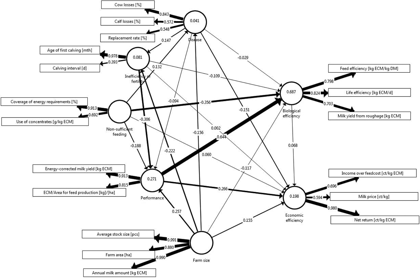
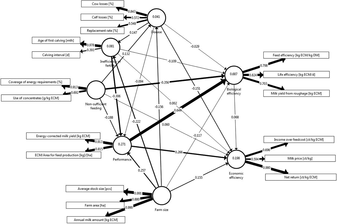
Calculated structural equation model for efficiency in milk production. Circles represent latent variables, rectangles represent measurement variables. Arrows between circles represent relationships between latent variables (path coefficients). Arrows between circles and rectangles represent indicator reliabilities (of the respective measurement variables). Numbers in circles represent the coefficient of determination (which is only calculated in case of endogenous variables). See Fig. 1 for a more general scheme of a structural equation model and more general explanations. See Table 2 for an overview of the latent variables and their associated measurement variables.
Data preparation and determinations for the model
In the first step, key areas for the cause and the effect sides of the model had to be defined. Since efficiency is within the scope of the current study, efficiency was set at the effect side (η) and sub-divided into the complexes biological efficiency (η 1) and economic efficiency (η 2). Biological efficiency was used to evaluate the quality of herd management. Economic efficiency was defined as the variable evaluating cost-related parameters from marginal and full-cost accounting. In the next step, the most important areas determining efficiency had to be identified to define the latent variables of the cause side (ξ). These areas were supposed to play a role in both the economic evaluation and evaluation of herd management. Health (Mitev et al., Reference Mitev, Gergovska, Miteva and Penev2011; Kvapilik et al., Reference Kvapilik, Hanuš, Bartoň, Klimešová and Roubal2015), fertility (Groenendaal et al., Reference Groenendaal, Galligan and Mulder2004; De Vries, Reference De Vries2006; Knapp et al., Reference Knapp, Laur, Vadas, Weiss and Tricarico2014) and feeding (Moran, Reference Moran and Moran2005) are the fields most recently mentioned in the literature to be of relevance for efficiency in milk production. As all these three fields have an influence on the performance of dairy cows, performance was also added as a field influencing efficiency (Stankov et al., Reference Stankov, Stoyanova and Petrov2015). In other efficiency studies (Mathijs and Swinnen, Reference Mathijs and Swinnen2001; Steinfeld et al., Reference Steinfeld, Wassenaar and Jutzi2006; MacDonald et al., Reference MacDonald, O'Donoghue, McBride, Nehring, Sandretto and Mosheim2007), economies of scale played a role in the efficiency of dairy farms, which means that for farmers who produce efficiently, costs decline as output expands. Thus, in the current study, farm size needed to be examined as a cause field (Stankov et al., Reference Stankov, Stoyanova and Petrov2015) in addition to health, fertility, feeding and performance. Emanating from that, each of the five cause variables was connected to each of the two effect variables using an arrow pointing from the cause to the effect variable, respectively. Based on the literature review (see above), additional relationships were determined between the five cause variables as well as the direction of causality for every single relationship. Furthermore, an influence of biological efficiency on economic efficiency was hypothesized, to be investigated by the SEM.
The software package SAS® 9.4 was used for data cleansing and for the calculation of descriptive statistics. The SAS® procedure PROC PLS (SAS Institute Inc., 2008) was applied to plot the variable importance of 30 variables (structural parameters, economic parameters and biological performance) according to their relevance for both biological and economic efficiency. The variable importance of projection score (VIP) summarizes the contribution a variable makes to the investigated model. The threshold for the VIP was set at ⩾0.8, hence, variables with values below that threshold have an insignificant influence on the model (Wold, Reference Wold and van der Waterbeemd1994). Based on the results of the VIP, the following decision rules were developed to decide on the selection of measurement variables for the respective latent variables step by step and by following the order of precedence mentioned:
(1) The results of VIP using PROC PLS in SAS (⩾ 0.8) are assessed.
(2) If two parameters are available which measure a similar phenomenon, only the one with the higher VIP is chosen.
(3) The variable has to have <0.15 of missing values, following the advice of Hair et al. (Reference Hair, Hult, Ringle and Sarstedt2014).
(4) There has to be a range of at least 0.30 between the minimum and maximum values within a measurement variable.
(5) Cost-related parameters are only allowed as effect variables, not as cause variables.
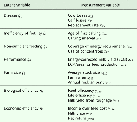
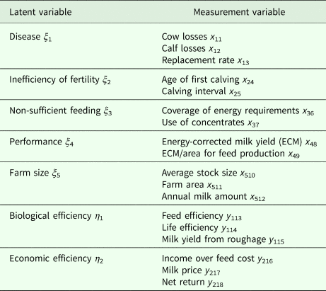
Based on the results of the VIP and the decision rules mentioned above, in the next step, the selected measurement variables were allocated to the corresponding latent variables. Therefore, two to three measurement variables were used to estimate the respective latent variable. In three cases (health, fertility and feeding), a negative value for the latent variable (disease, inefficiency of fertility [where increased age at first calving and increased calving interval are manifestations of inefficient fertility (management) on farms], non-sufficient feeding) was necessary to ensure correct characterization of the estimated field. Thus, five latent variables (disease ξ 1, inefficiency of fertility ξ 2, non-sufficient feeding ξ 3, performance ξ 4 and farm size ξ 5) were used as cause variables and two latent variables (biological efficiency η 1 and economic efficiency η 2) as effect variables. See Table 2 for an overview of the latent variables and their associated measurement variables.
Overview of the latent variables and their associated measurement variables. Each of the latent variables is estimated by two to three measurement variables; with latent cause variables ξ i, latent effect variables η j, measurement variables for latent cause variables x in, measurement variables for latent cause variables y jn; where i stands for the number of the latent cause variable, j stands for the number of the latent effect variable, n stands for the overall number of the measurement variable (consecutive numbering)
Assessment of the structural equation model
The SmartPLS 3.0 software (Ringle et al., Reference Ringle, Wende and Becker2015) was used to construct and calculate the SEM. The evaluation was based on a set of non-parametric evaluation criteria as recommended by Hair et al. (Reference Hair, Hult, Ringle and Sarstedt2014). The indicator reliability λ n (Hair et al., Reference Hair, Hult, Ringle and Sarstedt2014) was used to assess how sufficient a latent variable is estimated by a measurement variable. The composite reliability (ρ c) was applied as a measure of internal consistency. ρ c was supposed to adopt values of ⩾0.6, as recommended by Henseler et al. (Reference Henseler, Ringle, Sinkovics, Sinkovics and Ghauri2009). The average variance extracted (AVE [Fornell and Larcker, Reference Fornell and Larcker1981]) was used as a criterion for the assessment of convergent validity. The AVE describes to what extent a latent construct explains the variance of its measurement variables. A coefficient for AVE has to be ⩾0.5, following the advice of Henseler et al. (Reference Henseler, Ringle, Sinkovics, Sinkovics and Ghauri2009) and a measurement model reaching this threshold is considered as valid (Henseler et al., Reference Henseler, Ringle, Sinkovics, Sinkovics and Ghauri2009). The cross loadings offer another check in case of validity problems (Hair et al., Reference Hair, Hult, Ringle and Sarstedt2014). They describe the correlation of an indicator with other constructs in the model. If an indicator has a higher correlation with another latent variable than with its respective latent variable, the appropriateness of the model should be reconsidered.
The coefficient of determination (R 2) describes to what extent the constructed model was able to explain the variance in the respective latent variables. Chin (Reference Chin and Marcoulides1998) describes R 2 of 0.19, 0.33 and 0.67 as weak, moderate and substantial, respectively. Using path coefficients (γ), the hypotheses stated a priori are verified or disproved. To do so, the sign and magnitude of a path coefficient must be taken into account (Henseler et al., Reference Henseler, Ringle, Sinkovics, Sinkovics and Ghauri2009). Path coefficients can adopt values between −1 and 1. Path coefficients with values of |⩾0.2| were assessed as relevant (Chin, Reference Chin and Marcoulides1998) since they enable a statistically reliable statement about the relationship between the two investigated parameters in case they are significant (P ⩽ 0.05) according to the bootstrapping procedure (Hair et al., Reference Hair, Hult, Ringle and Sarstedt2014). A statement regarding the significance of all the evaluation criteria used (λ n, ρ c, AVE for the measurement models and R 2, γ i for the structural model) was made by the results of a non-parametric bootstrap procedure (Efron and Tibshirani, Reference Efron and Tibshirani1993; Davison and Hinkley, Reference Davison and Hinkley1997). The principle of bootstrapping is to collect a definite number of sub-samples with replacement from the original sample, and to estimate a model for each sub-sample (Hair et al., Reference Hair, Hult, Ringle and Sarstedt2014). As recommended by Ringle et al. (Reference Ringle, Wende and Becker2015), 5000 bootstrap runs were conducted to estimate the standard error. The theoretical t-value for significance of the evaluation criteria described above was set at 1.96 (P ⩽ 0.05).
As an additional method to prove validity of the results, split-half consistency was applied (Martin and Bateson, Reference Martin and Bateson2007). In doing so, two scenarios of splitting the data set into two groups were investigated, using the same model. After applying the SEM to the original data set (scenario original, n = 943), the years scenario was applied as a first approach by splitting the data set into the marketing years 2012 (scenario year 2012: n = 480) and 2013 (scenario year 2013: n = 463). As a second approach (scenario random), the data were split randomly and evenly into two groups (scenario random 1: n = 471, scenario random 2: n = 472) using the SAS® (SAS Institute Inc., 2008) procedure PROC SURVEYSELECT. Each of the scenarios was calculated in a single SEM, evaluated separately and compared with the results from the original scenario by using the same evaluation criteria.
Results
Calculated structural equation model
The SEM estimated 19 relationships between seven latent variables. Hence, 19 arrows connecting two latent variables, respectively, are shown in Fig. 2. All in all, there are 18 measurement variables which are associated with latent variables, and which allow an estimation of their respective latent variable.
Assessment of the measurement models
The results of three assessment criteria of the measurement models (λ n, ρ c, AVE) were evaluated in order to make a statement concerning reliability and validity of the measurement models. The indicator reliability λ n (see the values attached to the arrows in the respective measurement models in Fig. 2) was assessed as the first criterion. For disease (ξ 1), the associated measurement variable cow losses (x 11) had the highest indicator reliability (λ 1 = 0.843) of all three measurement variables. Thus, x 11 was the measurement variable, which was most appropriate to estimate disease. For the inefficiency of fertility (ξ 2), age of first calving (λ 4 = 0.978) estimated the latent variable better than calving interval (λ 5 = 0.393). Non-sufficient feeding (ξ 3) was best estimated by coverage of energy requirements (λ 6 = 0.913). For performance (ξ 4), both measurement variables, ECM (λ 8 = 0.913) as well as ECM/area for feed production (λ 9 = 0.815), were appropriate to estimate performance according to the recommendations of Hair et al. (Reference Hair, Hult, Ringle and Sarstedt2014). The latent variables farm size (ξ 5) and biological efficiency (η 1) were estimated appropriately by all of their associated measurement variables, respectively, since all measures for λ n were ⩾0.7 (Fig. 2). Out of the three measurement variables used to estimate biological efficiency, life efficiency (λ 14 = 0.824) was identified as the measurement variable most appropriate to estimate this latent variable. Economic efficiency (η 2) was also estimated by three measurement variables, of which net return (λ 18 = 0.980) estimated this latent variable most appropriately. Emanating from λ n, 14 out of 18 measurement variables were considered reliable for estimation of the respective associated latent variable.
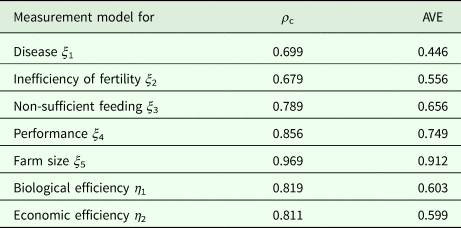
In the next step, the reliability of the seven single measurement models was assessed by using the composite reliability ρ c (Henseler et al., Reference Henseler, Ringle, Sinkovics, Sinkovics and Ghauri2009): Table 3 shows the results for ρ c. The measurement model inefficiency of fertility had the lowest composite reliability (ρ c = 0.679), whereas farm size had the highest composite reliability (ρ c = 0.969). As ρ c ⩾ 0.6 for all seven measurement models, all measurement models were proven to be reliable. All coefficients for ρ c were significant according to the bootstrapping procedure (t ⩾ 1.96).
Composite reliability (ρ c) and average variance extracted (AVE)
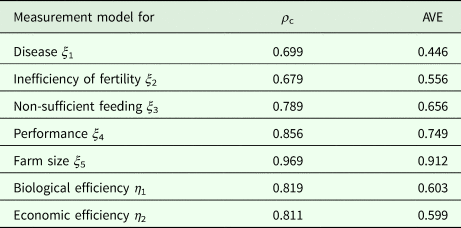
The AVE was used as a measure of validity. For all measurement models apart from disease, AVE was >0.5 (Table 3), proving the validity of all these measurement models (Henseler et al., Reference Henseler, Ringle, Sinkovics, Sinkovics and Ghauri2009). The measure for disease (AVE = 0.446) was the lowest of all measurement models and was just below the set threshold. The coefficients for AVE were significant for all latent variables, according to the bootstrapping procedure (t ⩾ 1.96).
Assessment of the structural model
Assessment of the structural model was conducted as the second step (Fig. 2). From the 19 relational paths considered, 15 were statistically significant (P ⩽ 0.05, if γ |⩾0.1|) and six relationships were statistically relevant (γ ⩾ |0.2|; Chin, Reference Chin and Marcoulides1998). Performance was the most important parameter for both biological and economic efficiency (Fig. 2). Greater performance resulted in greater biological and economic efficiency. Performance played a more important role for biological (γ 41 = 0.644) than for economic efficiency (γ 42 = 0.266). Non-sufficient feeding was identified as a second parameter of importance for biological efficiency. That is, better feeding of the cows on a farm leads to greater biological efficiency of the farm as a whole (γ 31 = −0.356). Performance was influenced mainly by the inefficiency of fertility and farm size. More efficient fertility on a farm led to better performance (γ 24 = −0.306) and larger farms also performed better, meaning they had higher total milk yield and also higher milk yield related to the feed area (γ 54 = 0.257). Larger farms were more efficient concerning fertility (γ 52 = −0.222).
Results for the coefficient of determination (R 2) were as follows: the model explained 0.27 of the variance in performance, 0.69 of the variance in biological efficiency and 0.20 of the variance in economic efficiency (Fig. 2). Thus, the model explained more than three times higher proportion of the variance in biological efficiency than in economic efficiency.
Split-half scenarios
In this section, the results of the split-half scenarios are assessed and compared with the original scenario (n = 943, including the marketing years 2012 and 2013) analysed above. Hereby, in the first scenario (scenario years), the data set was sub-divided into the marketing years 2012 (scenario year 2012) and 2013 (scenario year 2013). In the second scenario (scenario random), the data set was split randomly into two even groups (scenario random 1 and random 2).
Scenario years
For 17 out of the 18 measurement variables, λ n was very similar for both the scenario years 2012 and 2013. Only for milk price was λ n considerably lower in scenario years 2012 (λ 17 = 0.061) and 2013 (λ 17 = −0.273) than in the original scenario (λ 17 = 0.594). In the scenario years 2012 (ρ c = 0.6, AVE = 0.43) and 2013 (ρ c = 0.48, AVE = 0.43), ρ c and AVE for economic efficiency were considerably lower than in the original scenario (ρ c = 0.81, AVE = 0.59). For both the scenarios 2012 and 2013, the path coefficients (Chin, Reference Chin and Marcoulides1998) of the original scenario were also statistically relevant in these cases according to Chin (Reference Chin and Marcoulides1998). Furthermore, farm size had an influence on economic efficiency for the scenario year 2012 (γ 54 = 0.205). This relationship indicates that larger farms have a greater economic efficiency, which is consistent with previous studies (MacDonald et al., Reference MacDonald, O'Donoghue, McBride, Nehring, Sandretto and Mosheim2007). Moreover, non-sufficient feeding played a role in performance (γ 34 = −0.213 for scenario year 2012). This relationship estimates a higher performance for farms with better feeding. Greater economic efficiency was estimated for farms with less disease (γ 12 = −0.207 for 2012). For both the scenario years 2012 and 2013, a considerably higher proportion of the variance of economic efficiency was explained by the model (R 2 = 0.29 for scenario year 2012; R 2 = 0.32 for scenario year 2013) compared with the original scenario (R 2 = 0.20).
Scenario random
For both the scenarios random 1 and random 2, λ n was very similar to the original scenario for all 18 measurement variables. In both the scenarios, ρ c and AVE are within the same range compared with the original scenario. Also, for both scenarios, the path coefficients (Chin, Reference Chin and Marcoulides1998) of the original scenario were also statistically relevant in these cases, according to Chin (Reference Chin and Marcoulides1998). Additionally, the statistically relevant path coefficients were in a similar dimension compared with the original scenario, except for the relationship between non-sufficient feeding and biological efficiency for scenario random 1. For this relationship, the absolute value of the path coefficient was higher (γ 31 = −0.490) compared with the original scenario (γ 31 = −0.356), indicating that non-sufficient feeding was of greater importance for biological efficiency in the model of scenario random 1. Furthermore, five additional statistically relevant relationships were observed in scenario random 1 that were not statistically relevant in the original scenario. Farm size had an influence firstly on economic efficiency (γ 54 = 0.297) and secondly on disease (γ 51 = −0.223). Additionally, farms with less disease showed greater efficiency of fertility (γ 12 = 0.215). Greater biological efficiency was observed (γ 21 = −0.301) on farms with more efficient fertility. Moreover, non-sufficient feeding played a role in performance in scenario random 1 (γ 34 = −0.220). The results for R 2 (results not shown) were similar to the original scenario for the scenarios random 1 and random 2.
Discussion
Assessment of the measurement models
From the indicator reliability (λ n), 14 out of 18 measurement variables were considered reliable for estimation of the respective associated latent variable (Hair et al., Reference Hair, Hult, Ringle and Sarstedt2014). The indicator reliability for the measurement variables calf losses, replacement rate, calving interval and milk price were <0.7, respectively. Nevertheless, these measurement variables were kept in the model, since variables with indicator reliabilities between 0.4 and 0.7 should only be removed from the construct if their removal increases AVE above the threshold of 0.5 mentioned previously (Hair et al., Reference Hair, Hult, Ringle and Sarstedt2014). This was not the case, as shown by the individually performed analyses for each of the measurement variables mentioned. For a more comprehensive estimation of fertility, additional indicators such as the insemination index or the non-return-rate should be added in future studies; however, these were not available in the current study. All values for the composite reliability (ρ c) were >0.6, which is interpreted as reliable following the recommendation of Henseler et al. (Reference Henseler, Ringle, Sinkovics, Sinkovics and Ghauri2009). These results show that all seven latent variables are measured sufficiently by their respective measurement variables. The AVE for six out of the seven measurement models is above the recommended threshold (Henseler et al., Reference Henseler, Ringle, Sinkovics, Sinkovics and Ghauri2009) and that for the latent variable disease is 0.446, which is just below the mentioned threshold. One reason for the low AVE is the low indicator reliability of the measurement variables calf losses and replacement rate. Since disease is not sufficiently estimated by two out of its three measurement variables, this indicates a lack of sufficient estimation of the whole latent variable disease. Thus, other or additional measurement variables could be necessary to supplement the estimation of disease. In the current study, additional measurement variables were not available from the data sets. However, the cross loadings were used for an additional check, as recommended in case of validity problems (Hair et al., Reference Hair, Hult, Ringle and Sarstedt2014). Since correlations between the measurement variables (calf losses and replacement rate) with their latent variable disease were higher than the correlation with other latent variables, the measurement model for disease was nevertheless appropriate.
Assessment of the structural model
Three statistically relevant relationships between cause variables were identified. Farm size had an influence on both performance (γ 54 = 0.257) and the inefficiency of fertility (γ 52 = −0.222), meaning that larger farms had better performance and fertility. Due to economies of scale, an increase in farm size led to greater productivity, as also seen in other studies (Steinfeld et al., Reference Steinfeld, Wassenaar and Jutzi2006; MacDonald et al., Reference MacDonald, O'Donoghue, McBride, Nehring, Sandretto and Mosheim2007). Additionally, the inefficiency of fertility influenced performance (γ 24 = −0.306); hence, farms with a greater efficiency of fertility also had better performance. A positive relation between fertility and performance was also found in several previous studies (Groenendaal et al., Reference Groenendaal, Galligan and Mulder2004; De Vries, Reference De Vries2006; Knapp et al., Reference Knapp, Laur, Vadas, Weiss and Tricarico2014). There was no statistically relevant relationship concerning disease found in the SEM, which is probably due to the insufficient estimation of this latent variable. There were three statistically relevant relationships observed between cause and effect variables. Performance was the most important parameter for both biological and economic efficiency. Better performance resulted in greater biological and economic efficiency. A positive relationship between performance and efficiency in milk production was also found in previous studies (Bailey et al., Reference Bailey, Hardin, Spain, Garrett, Hoehne, Randle, Ricketts, Steevens and Zulovich1997; Marston et al., Reference Marston, Clark, Anderson, Kersbergen, Lunak, Marcinkowski, Murphy, Schwab and Erickson2011; Stankov et al., Reference Stankov, Stoyanova and Petrov2015). Performance played a more important role for biological (γ 41 = 0.644) than for economic efficiency (γ 42 = 0.266) in this model. Biological efficiency was affected by non-sufficient feeding (γ 31 = −0.356), whereas economic efficiency was not affected by non-sufficient feeding. Usually, feeding costs are at least half of the overall production costs of a dairy farm (Moran, Reference Moran and Moran2005) and therefore feeding would be expected to play a role in economic efficiency. However, in the current study, cost-related variables were only included as effect variables, since information on monetary aspects was incomplete or unavailable for the cause variables. Thus, the estimation of non-sufficient feeding in the current study is due rather to evaluation of the feeding management as a component of herd management, i.e. the biological parameters, than it is due to evaluation of the feeding costs. Nevertheless, indirectly, these parameters also allow an evaluation of efficient feed use. For example, if the coverage of energy requirements is >100%, the risk of a cow's body condition score being above the optimum increases, without additionally making more profit from the higher amount of feed used. One reason for the non-existent influence of feeding on the economic efficiency might be that feeding was not estimated comprehensively by the measurement variables coverage of energy requirements and the use of concentrates. Additional meaningful parameters such as the urea content of milk as an indicator of a balanced ratio of energy and protein supply (Huhtanen and Nousiainen, Reference Huhtanen and Nousiainen2012; Mgbeahuruike et al., Reference Mgbeahuruike, Nørgaard, Eriksson, Nordqvist and Nadeau2016) or further information on the composition of concentrates in the ration were not available, but should be considered in future studies, if possible.
Significant correlations between life efficiency and profit were found in the studies of Wangler and Harms (Reference Wangler and Harms2006). Thus, a correlation between biological efficiency and economic efficiency was also expected in the current study, as life efficiency is an important measurement variable of biological efficiency and net return was identified as the key measurement variable for economic efficiency. Nevertheless, there was no relationship between the two effect variables found in the current study. However, fluctuations in the milk price most likely mask the relationship between biological and economic efficiency. Therefore, an additional scenario with an identical milk price was calculated to prove whether the relationship was stronger in this case (see ‘Split-half scenarios’ below).
The model explained a substantial proportion (Chin, Reference Chin and Marcoulides1998) of the variance in biological efficiency (0.69) and a smaller proportion of the variance in economic efficiency (0.20). Thus, the coefficient of determination was more than three times higher for biological efficiency than for economic efficiency, implying a more appropriate eligibility of biological parameters for the evaluation of efficiency, considering this data set. Biological efficiency is used as a parameter to evaluate the quality of herd management, which has gained in importance especially in intensive farming systems. Approximately 45–50% of the increase in milk yields under intensive management has been achieved through improvements in management practices (Hansen, Reference Hansen2000; VanRaden, Reference VanRaden2004; Shook, Reference Shook2006).
Split-half scenarios
Different scenarios for a split-half consistency were conducted in order to evaluate the reproducibility of the results (Ombao et al., Reference Ombao, Lindquist, Thompson and Aston2017). The aim of doing so was, in general, to test SEM for robustness in case of changes in input data. Particularly in the case of splitting the data into the marketing years, it was done to observe the influence of annual fluctuations (e.g. in the milk price or the quality of feeds) on the model and the calculated interactions.
For both the scenario years 2012 and 2013, the indicator reliability for milk price (λ 17) was considerably lower compared with the original scenario. This noticeable fluctuation in the results for milk price occurred due to the very different range in milk prices between the years (year 2012: 29–37 cents/kg milk; year 2013: 38–46 cents/kg milk). In 2012, λ n for milk price as a partial measure of economic efficiency was not statistically significant (λ n = 0.061, P = 0.634). In 2013, which was the only one out of five models tested with a negative relationship between milk price and economic efficiency (λ n = −0.273, P = 0.003), the whole latent variable economic efficiency was not sufficiently measured by its indicators according to the measurement model assessment criteria (ρ c = 0.48; AVE = 0.43). Therefore, the results of the split-half scenarios by years are not statistically valid.
An additional scenario with an identical milk price was calculated in order to investigate the influence of fluctuations in the milk price on the relationship between biological and economic efficiency. This model used the same input data as the main model apart from the milk price and the related parameters income over feed cost and net return (here the identical milk price was also included in the new calculation of the respective parameters). Interestingly, with an identical milk price, the relationship between biological and economic efficiency became stronger and was statistically significant in this new scenario (γ 12 = 0.157, P < 0.05) compared with the main model (γ 12 = 0.068, P > 0.05).
Evaluation of the results in relation to other efficiency studies
In several agricultural efficiency studies, economies of scale were found to play an important role. This means that declining production costs accompany increasing scales of operation (Steinfeld et al., Reference Steinfeld, Wassenaar and Jutzi2006). In studies by MacDonald et al. (Reference MacDonald, O'Donoghue, McBride, Nehring, Sandretto and Mosheim2007), the costs of housing, milking facilities and machinery fell while the net return rose. In the current study, economies of scale could not be proven. Farm size was related indirectly to economic efficiency via performance, since larger farms can reach higher yields (γ 54 = 0.257) and performance (as the latent variable to measure yield) was related positively to economic efficiency (γ 42 = 0.266). Stankov et al. (Reference Stankov, Stoyanova and Petrov2015) found a correlation between farm size and profit (r = 0.72) and between milk yield and profit (r = 0.72). The latter relationship was also observed in the current study. A relationship between dairy farm size and productivity was also found by Weersink and Tauer (Reference Weersink and Tauer1991).
In a study on environmental efficiency conducted by Knapp et al. (Reference Knapp, Laur, Vadas, Weiss and Tricarico2014), improvements in disease and fertility management contributed to an increase in feed efficiency and lifetime productivity of single cows and whole dairy herds. Among other things, reduced culling rates reduced the requirement for replacement cows and therefore increased dairy profitability as well. In the current study, no significant relationship was found between disease and efficiency or between fertility and efficiency. In previous studies, a relationship was found between disease and performance. Mastitis (de los Campos et al., Reference de los Campos, Gianola and Heringstad2006) and lameness (Mitev et al., Reference Mitev, Gergovska, Miteva and Penev2011) were accompanied by a reduction in milk yield. In the current study, no significant relationship between disease and performance was found.
Concluding statement
The current study is one of the first investigations using the method of PLS-SEM in the evaluation of efficiency in milk production. This method enabled an estimation of efficiency, including the different approaches towards economic efficiency and biological efficiency, which are latent variables and therefore not themselves measurable. In the current study, efficiency was determined mostly by performance, which was of higher importance for biological than for economic efficiency. Economies of scale were proven since larger farms were able to be more efficient concerning performance and fertility.
The identification of meaningful measurement variables for a comprehensive estimation of both cause and effect variables is challenging and decisive for a reliable and valid PLS-SEM. In future studies, the inclusion of additional meaningful measurement variables for a more comprehensive estimation of the latent variables fertility and disease is recommended.
Financial support
We gratefully acknowledge funding by the Stiftung Schleswig-Holsteinische Landschaft, the Gesellschaft für Energie und Klimaschutz Schleswig-Holstein GmbH (EKSH) and the Landwirtschaftliche Rentenbank.
Conflict of interest
None.
Ethical standards
Not applicable.