1 Introduction
In contrast to normal Brownian diffusion in liquids, tracer diffusion in complex systems such as colloidal suspensions is strongly hindered and anomalous (Wang et al. Reference Wang, Kuo, Bae and Granick2012; Metzler et al. Reference Metzler, Jeon, Cherstvy and Barkai2014). Modelling such systems is challenging owing to competing nonlinear effects, including long-range viscous interactions between the tracer particles and host matrix. In this work some progress is made in the case of a hard-sphere suspension containing spherical tracer particles in the pore fluid. Batchelor (Reference Batchelor1976, Reference Batchelor1983, Reference Batchelor1986) solved the hydrodynamic equations describing this system in the dilute limit and obtained expressions for the diffusion coefficients to first order in the particle volume fractions. Later researchers obtained similar results starting from the Smoluchowski and Fokker–Planck equations (Zhang & Nagele Reference Zhang and Nagele2002; Bruna & Chapman Reference Bruna and Chapman2012) or by using thermodynamic methods (Vergara et al. Reference Vergara, Paduano, Vitagliano and Sartorio2001; Annunziata Reference Annunziata2008), while recent efforts have employed Stokesian and molecular dynamics simulations (Wang & Brady Reference Wang and Brady2015; Hannam, Daivis & Bryant Reference Hannam, Daivis and Bryant2017). In many ‘crowded’ systems the host particles are at non-dilute volume fractions near to and above the glass transition, where long-range viscous effects and nonlinear particle–particle interactions are predominant (Wang et al. Reference Wang, Kuo, Bae and Granick2012; Guan, Wang & Granick Reference Guan, Wang and Granick2014; Sentjabrskaja et al. Reference Sentjabrskaja, Zaccarelli, Michele, De Sciortino, Tartaglia, Voigtmann, Egelhaaf and Laurati2016). In order to obtain expressions for the diffusion coefficients at these high concentrations, here a phenomenological approach is used, in which non-equilibrium thermodynamics is combined with capillary flow models and empirical data.
In § 2 the irreversible thermodynamics equations describing cross-diffusion are described, and Batchelor’s theory of multicomponent diffusion is briefly reviewed. In § 3 the equations are written in a membrane transport framework in order to obtain expressions for the diffusion coefficients in terms of experimentally convenient quantities such as the permeability and osmotic pressure. Expressions for these quantities are combined in § 4 with Batchelor’s results to obtain the diffusion coefficients as functions of the host-particle volume fraction. Section 5 presents some results and comparison with experiment; § 6 contains a discussion of sedimentation and the Stokes–Einstein equation, and the physical interpretation and measurement of parameters.
2 Diffusion and cross-diffusion in hard-sphere suspensions
2.1 Flux equations
From irreversible thermodynamics (deGroot & Mazur Reference de Groot and Mazur1962; Batchelor Reference Batchelor1986) the diffusion fluxes in a binary hard-sphere suspension can be written as
 $$\begin{eqnarray}\displaystyle & \displaystyle \boldsymbol{J}_{1}=-\unicode[STIX]{x1D613}_{11}\unicode[STIX]{x1D735}\unicode[STIX]{x1D707}_{1}-\unicode[STIX]{x1D613}_{12}\unicode[STIX]{x1D735}\unicode[STIX]{x1D707}_{2}, & \displaystyle\end{eqnarray}$$
 $$\begin{eqnarray}\displaystyle & \displaystyle \boldsymbol{J}_{2}=-\unicode[STIX]{x1D613}_{21}\unicode[STIX]{x1D735}\unicode[STIX]{x1D707}_{1}-\unicode[STIX]{x1D613}_{22}\unicode[STIX]{x1D735}\unicode[STIX]{x1D707}_{2}, & \displaystyle\end{eqnarray}$$
 $\unicode[STIX]{x1D613}_{ij}$
are phenomenological coefficients,
 $\boldsymbol{J}_{i}=n_{i}(\boldsymbol{u}_{i}-\boldsymbol{u})$
is the flux of
 $i$
moving at average velocity
 $\boldsymbol{u}_{i}$
relative to the volume-average velocity
 $\boldsymbol{u}$
of the mixture and
 $n_{i}$
is the concentration of
 $i$
(number of particles per unit volume of mixture). If the system is not too far from equilibrium, the
 $\unicode[STIX]{x1D613}_{ij}$
obey the Onsager relation (deGroot & Mazur Reference de Groot and Mazur1962; Batchelor Reference Batchelor1986)
 $$\begin{eqnarray}\unicode[STIX]{x1D613}_{12}=\unicode[STIX]{x1D613}_{21}.\end{eqnarray}$$
In (2.1)
 $\unicode[STIX]{x1D707}_{i}=\unicode[STIX]{x1D707}_{i}^{a}-v_{i}\unicode[STIX]{x1D707}_{0}^{a}/v_{0}$
are effective (reduced) chemical potentials, where
 $\unicode[STIX]{x1D707}_{i}^{a}$
is the actual chemical potential per particle of component
 $i$
(0 is the fluid, assumed incompressible, 1 is the host particles and 2 is the tracer particles) and
 $v_{i}=(4/3)\unicode[STIX]{x03C0}R_{i}^{3}$
is the volume of a particle of radius
 $R_{i}$
. When the suspending fluid is incompressible and composed of molecules that are much smaller than the hard-sphere particles, the reduced chemical potentials in a hard-sphere suspension are equivalent to the chemical potentials of a hard-sphere gas at the same volume fractions (Batchelor Reference Batchelor1983; Russel, Seville & Schowalter Reference Russel, Seville and Schowalter1989; Annunziata Reference Annunziata2008).
At constant mixture pressure
 $P$
and temperature
 $T$
the chemical potentials depend on the concentrations
 $n_{1}$
and
 $n_{2}$
, so that
 $$\begin{eqnarray}\displaystyle & \displaystyle \unicode[STIX]{x1D735}\unicode[STIX]{x1D707}_{1}=\unicode[STIX]{x1D707}_{11}\unicode[STIX]{x1D735}n_{1}+\unicode[STIX]{x1D707}_{12}\unicode[STIX]{x1D735}n_{2}, & \displaystyle\end{eqnarray}$$
 $$\begin{eqnarray}\displaystyle & \displaystyle \unicode[STIX]{x1D735}\unicode[STIX]{x1D707}_{2}=\unicode[STIX]{x1D707}_{21}\unicode[STIX]{x1D735}n_{1}+\unicode[STIX]{x1D707}_{22}\unicode[STIX]{x1D735}n_{2}, & \displaystyle\end{eqnarray}$$
 $\unicode[STIX]{x1D707}_{ij}=(\unicode[STIX]{x2202}\unicode[STIX]{x1D707}_{i}/\unicode[STIX]{x2202}n_{j})_{T,P,n_{k\neq j}}$
. Equations (2.1) can then be written as
 $$\begin{eqnarray}\displaystyle & \displaystyle \boldsymbol{J}_{1}=-D_{11}\unicode[STIX]{x1D735}n_{1}-D_{12}\unicode[STIX]{x1D735}n_{2}, & \displaystyle\end{eqnarray}$$
 $$\begin{eqnarray}\displaystyle & \displaystyle \boldsymbol{J}_{2}=-D_{21}\unicode[STIX]{x1D735}n_{1}-D_{22}\unicode[STIX]{x1D735}n_{2}, & \displaystyle\end{eqnarray}$$
 $D_{ij}$
are
 $$\begin{eqnarray}D_{11}=\unicode[STIX]{x1D613}_{11}\unicode[STIX]{x1D707}_{11}+\unicode[STIX]{x1D613}_{12}\unicode[STIX]{x1D707}_{21},\quad D_{12}=\unicode[STIX]{x1D613}_{11}\unicode[STIX]{x1D707}_{12}+\unicode[STIX]{x1D613}_{12}\unicode[STIX]{x1D707}_{22},\end{eqnarray}$$
 $$\begin{eqnarray}D_{21}=\unicode[STIX]{x1D613}_{21}\unicode[STIX]{x1D707}_{11}+\unicode[STIX]{x1D613}_{22}\unicode[STIX]{x1D707}_{21},\quad D_{22}=\unicode[STIX]{x1D613}_{21}\unicode[STIX]{x1D707}_{12}+\unicode[STIX]{x1D613}_{22}\unicode[STIX]{x1D707}_{22}.\end{eqnarray}$$
Here
 $D_{11}$
is the main Fickian diffusion coefficient of the host particles, while
 $D_{12}$
is a cross-diffusion coefficient characterizing motion of the host particles caused by a gradient in tracer particle concentration
 $\unicode[STIX]{x1D735}n_{2}$
. Similarly,
 $D_{22}$
is the Fickian tracer diffusivity, while
 $D_{21}$
accounts for motion of the tracer particles caused by a gradient in
 $n_{1}$
.
2.2 Batchelor’s theory
By calculating the bulk mobilities of spherical particles in a polydisperse suspension, Batchelor (Reference Batchelor1983, Reference Batchelor1986) derived expressions for the phenomenological coefficients
 $\unicode[STIX]{x1D613}_{ij}$
to first order in the volume fractions
 $\unicode[STIX]{x1D719}_{i}=v_{i}n_{i}$
. For a bidisperse suspension in the dilute tracer limit (
 $\unicode[STIX]{x1D719}_{2}\ll \unicode[STIX]{x1D719}_{1}\ll 1$
) the
 $\unicode[STIX]{x1D613}_{ij}$
are
 $$\begin{eqnarray}\unicode[STIX]{x1D613}_{11}=\frac{n_{1}}{6\unicode[STIX]{x03C0}\unicode[STIX]{x1D702}_{0}R_{1}}(1+(K_{11}^{\prime }+K_{11}^{\prime \prime })\unicode[STIX]{x1D719}_{1}),\quad \unicode[STIX]{x1D613}_{12}=\frac{n_{1}}{6\unicode[STIX]{x03C0}\unicode[STIX]{x1D702}_{0}R_{1}}(\unicode[STIX]{x1D706}_{12}^{-3}K_{12}^{\prime \prime }\unicode[STIX]{x1D719}_{2}),\end{eqnarray}$$
 $$\begin{eqnarray}\unicode[STIX]{x1D613}_{21}=\frac{n_{2}}{6\unicode[STIX]{x03C0}\unicode[STIX]{x1D702}_{0}R_{2}}(\unicode[STIX]{x1D706}_{21}^{-3}K_{21}^{\prime \prime }\unicode[STIX]{x1D719}_{1}),\quad \unicode[STIX]{x1D613}_{22}=\frac{n_{2}}{6\unicode[STIX]{x03C0}\unicode[STIX]{x1D702}_{0}R_{2}}(1+K_{21}^{\prime }\unicode[STIX]{x1D719}_{1}),\end{eqnarray}$$
where
 $\unicode[STIX]{x1D702}_{0}$
is the viscosity of the suspending fluid and
 $\unicode[STIX]{x1D706}_{ij}=R_{j}/R_{i}.$
A fit to numerical data obtained over a range of
 $\unicode[STIX]{x1D706}_{ij}$
values leads to
 $K_{ij}^{\prime \prime }=\unicode[STIX]{x1D706}_{ij}^{2}/(1+\unicode[STIX]{x1D706}_{ij}^{3})-(\unicode[STIX]{x1D706}_{ij}^{2}+3\unicode[STIX]{x1D706}_{ij}+1)$
and
 $K_{ij}^{\prime }=-2.5/(1+b\unicode[STIX]{x1D706}_{ij})$
, where
 $b$
is a parameter (Batchelor Reference Batchelor1983). Here the value
 $b=0.22$
is used, as this gives a close match to known results when
 $\unicode[STIX]{x1D706}_{ij}=1$
; for example
 $K_{11}^{\prime }+K_{11}^{\prime \prime }=-6.55$
leading to (2.9a
) (Batchelor Reference Batchelor1976).
In the dilute limit, the binary hard-sphere gas chemical potentials are
 $$\begin{eqnarray}\displaystyle & \displaystyle \unicode[STIX]{x1D707}_{1}=\unicode[STIX]{x1D707}_{1}^{0}+k_{B}T(\ln \unicode[STIX]{x1D719}_{1}+b_{11}\unicode[STIX]{x1D719}_{1}+b_{21}\unicode[STIX]{x1D719}_{2}), & \displaystyle\end{eqnarray}$$
 $$\begin{eqnarray}\displaystyle & \displaystyle \unicode[STIX]{x1D707}_{2}=\unicode[STIX]{x1D707}_{2}^{0}+k_{B}T(\ln \unicode[STIX]{x1D719}_{2}+b_{22}\unicode[STIX]{x1D719}_{2}+b_{12}\unicode[STIX]{x1D719}_{1}), & \displaystyle\end{eqnarray}$$
 $k_{B}$
is Boltzmann’s constant,
 $\unicode[STIX]{x1D707}_{i}^{0}$
are constants (at constant
 $T,P$
) and
 $b_{ij}=(1+\unicode[STIX]{x1D706}_{ij})^{3}$
(Annunziata Reference Annunziata2008; Santos & Rorhmann Reference Santos and Rorhmann2013). Differentiating (2.7) with respect to
 $n_{i}$
gives
 $$\begin{eqnarray}\unicode[STIX]{x1D707}_{11}=k_{B}T(n_{1}^{-1}+v_{1}b_{11}),\quad \unicode[STIX]{x1D707}_{12}=k_{B}Tv_{2}b_{21},\end{eqnarray}$$
 $$\begin{eqnarray}\unicode[STIX]{x1D707}_{21}=k_{B}Tv_{1}b_{12},\quad \unicode[STIX]{x1D707}_{22}=k_{B}T(n_{2}^{-1}+v_{2}b_{22}).\end{eqnarray}$$
Combining (2.8) and (2.6) with (2.5) leads to Batchelor’s expressions for the diffusion coefficients, in the limit
 $\unicode[STIX]{x1D719}_{2}\ll \unicode[STIX]{x1D719}_{1}\ll 1,$
as
 $$\begin{eqnarray}D_{11}=D_{1}^{0}(1+1.45\unicode[STIX]{x1D719}_{1}),\quad D_{12}=D_{1}^{0}(b_{12}+K_{12}^{\prime \prime })\unicode[STIX]{x1D719}_{1},\end{eqnarray}$$
 $$\begin{eqnarray}D_{21}=D_{2}^{0}(b_{21}+K_{21}^{\prime \prime })\unicode[STIX]{x1D719}_{2},\quad D_{22}=D_{2}^{0}(1+K_{21}^{\prime }\unicode[STIX]{x1D719}_{1}),\end{eqnarray}$$
where
 $D_{i}^{0}=k_{B}T/6\unicode[STIX]{x03C0}\unicode[STIX]{x1D702}_{0}R_{i}$
is the Stokes–Einstein diffusivity of component
 $i$
.
3 Membrane transport formulation
Extending Batchelor’s theory to higher volume fractions of the host particles is challenging because of the difficulty of determining higher-order expressions for the phenomenological coefficients. However, progress can be made by rewriting the
 $\unicode[STIX]{x1D613}_{ij}$
and
 $\unicode[STIX]{x1D707}_{ij}$
in terms of the host-matrix permeability and osmotic pressure, for which experimental data and theoretical expressions are available.
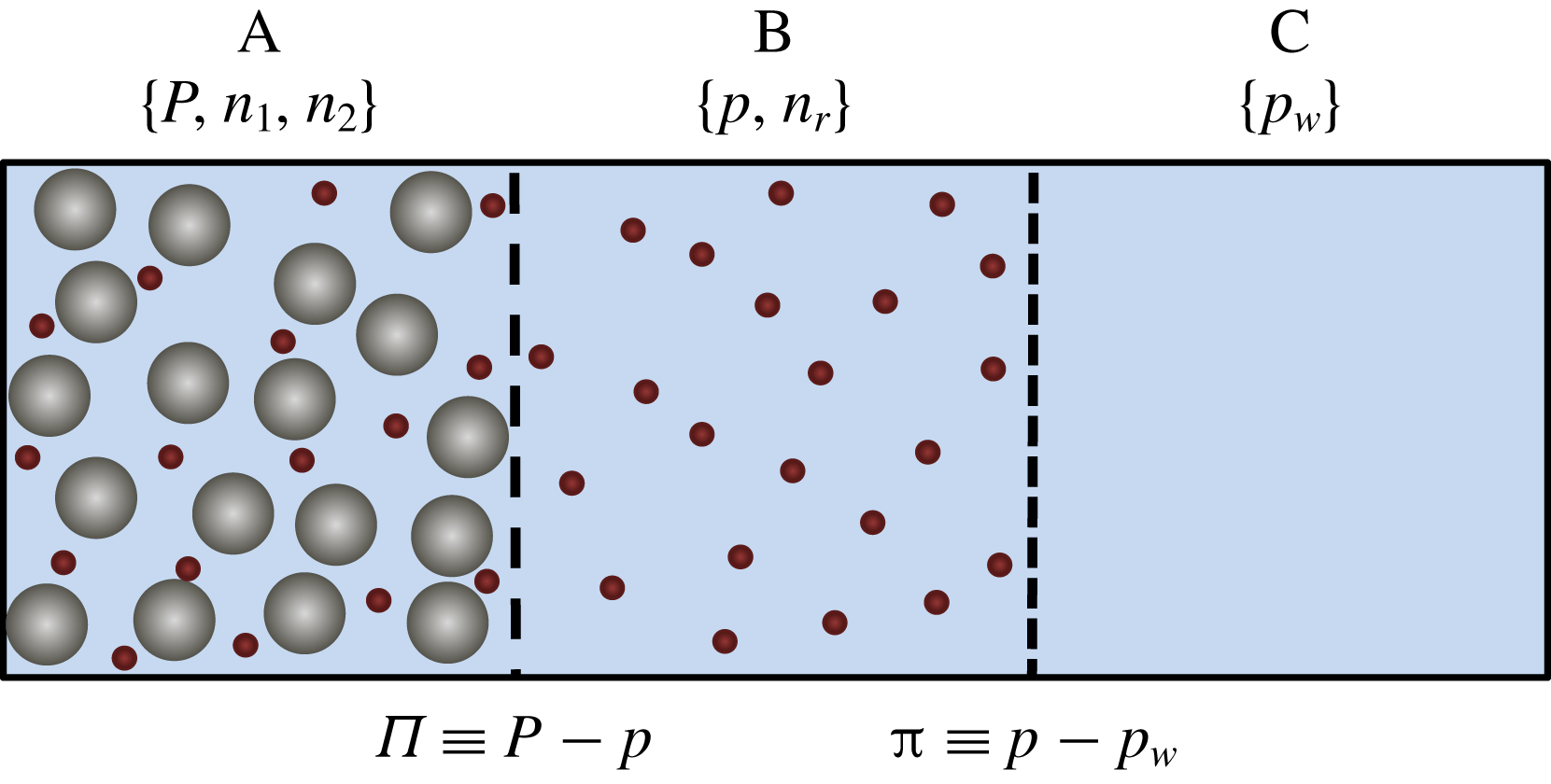
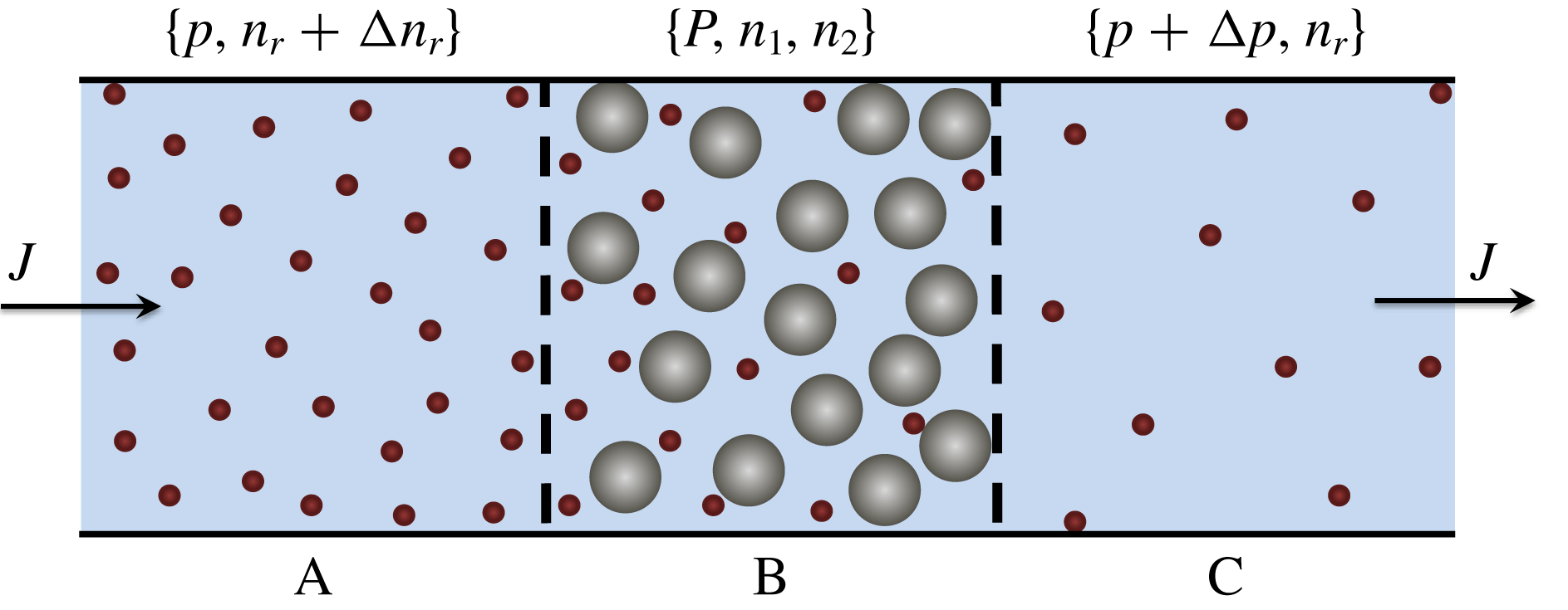
Illustration of osmotic equilibrium in a bidisperse hard-sphere suspension.
 $P$
is the total mixture pressure of the suspension in compartment A;
 $p$
is the pressure of the tracer suspension in B; and
 $p_{w}$
is the pressure of the pure fluid in C. The membrane separating compartments A and B is permeable to the fluid (blue) and tracer particles (red) but impermeable to the larger host particles (grey). The difference between the pressures in A and B is the host-particle osmotic pressure
 $\unicode[STIX]{x1D6F1}\equiv P-p$
. The membrane separating compartments B and C is permeable to the fluid but impermeable to the tracer particles; the tracer osmotic pressure is
 $\unicode[STIX]{x03C0}\equiv p-p_{w}$
. Because of excluded volume effects, the tracer concentration
 $n_{2}$
in compartment A is less than the concentration
 $n_{r}$
in the reservoir compartment B;
 $\unicode[STIX]{x1D6FC}=n_{2}/n_{r}$
is the equilibrium partition coefficient.

3.1 Osmotic equilibrium
The chemical potentials can be replaced with osmotic pressures by considering the osmotic equilibrium system illustrated in figure 1. The suspension in compartment A at pressure
 $P$
is in equilibrium across a semi-permeable partition with a reservoir at pressure
 $p$
(compartment B) containing only the fluid and tracer particles. Compartment B is in turn in equilibrium with another reservoir (compartment C) that contains only the suspending fluid at pressure
 $p_{w}.$
At equilibrium the tracer chemical potential
 $\unicode[STIX]{x1D707}_{2}$
in the suspension is equal to the chemical potential
 $\unicode[STIX]{x1D707}_{r}$
of the tracer particles in the reservoir, so that
 $$\begin{eqnarray}\unicode[STIX]{x1D707}_{2}=\unicode[STIX]{x1D707}_{r}.\end{eqnarray}$$
The Gibbs–Duhem equation applied to the suspension in A is, at constant
 $T$
,
 $$\begin{eqnarray}n_{1}\,\text{d}\unicode[STIX]{x1D707}_{1}+n_{2}\,\text{d}\unicode[STIX]{x1D707}_{2}=\text{d}\unicode[STIX]{x1D6F1}_{T},\end{eqnarray}$$
where
 $\unicode[STIX]{x1D6F1}_{T}\equiv P-p_{w}$
is the total osmotic pressure of the suspension. Equation (3.2) is a consequence of the analogy between hard-sphere fluids and hard-sphere suspensions, for which
 $\unicode[STIX]{x1D6F1}_{T}$
plays the role of pressure (Batchelor Reference Batchelor1983; Russel et al.
Reference Russel, Seville and Schowalter1989; Annunziata Reference Annunziata2008). The Gibbs–Duhem equation applied to the reservoir compartment B is
 $$\begin{eqnarray}n_{r}\,\text{d}\unicode[STIX]{x1D707}_{r}=\text{d}\unicode[STIX]{x03C0},\end{eqnarray}$$
where
 $\unicode[STIX]{x03C0}\equiv p-p_{w}$
is the tracer osmotic pressure. Combining (3.1)–(3.3) gives
 $$\begin{eqnarray}n_{1}\,\text{d}\unicode[STIX]{x1D707}_{1}=\text{d}\unicode[STIX]{x1D6F1}+(1-\unicode[STIX]{x1D6FC})\,\text{d}\unicode[STIX]{x03C0}\quad \text{and}\quad n_{2}\,\text{d}\unicode[STIX]{x1D707}_{2}=\unicode[STIX]{x1D6FC}\,\text{d}\unicode[STIX]{x03C0},\end{eqnarray}$$
where
 $\unicode[STIX]{x1D6FC}\equiv n_{2}/n_{r}$
is the equilibrium partition coefficient and
 $\unicode[STIX]{x1D6F1}\equiv P-p$
is the host-particle osmotic pressure. With the local equilibrium assumption (deGroot & Mazur Reference de Groot and Mazur1962), equation (3.4) can be written in terms of gradients as
 $$\begin{eqnarray}n_{1}\unicode[STIX]{x1D735}\unicode[STIX]{x1D707}_{1}=\unicode[STIX]{x1D735}\unicode[STIX]{x1D6F1}+(1-\unicode[STIX]{x1D6FC})\unicode[STIX]{x1D735}\unicode[STIX]{x03C0}\quad \text{and}\quad n_{2}\unicode[STIX]{x1D735}\unicode[STIX]{x1D707}_{2}=\unicode[STIX]{x1D6FC}\unicode[STIX]{x1D735}\unicode[STIX]{x03C0}.\end{eqnarray}$$
Differentiating with respect to
 $n_{i}$
gives
 $$\begin{eqnarray}\unicode[STIX]{x1D707}_{11}=n_{1}^{-1}(\unicode[STIX]{x1D6F1}_{1}+(1-\unicode[STIX]{x1D6FC})\unicode[STIX]{x03C0}_{1}),\quad \unicode[STIX]{x1D707}_{12}=n_{1}^{-1}(\unicode[STIX]{x1D6F1}_{2}+(1-\unicode[STIX]{x1D6FC})\unicode[STIX]{x03C0}_{2}),\end{eqnarray}$$
 $$\begin{eqnarray}\unicode[STIX]{x1D707}_{21}=n_{2}^{-1}\unicode[STIX]{x1D6FC}\unicode[STIX]{x03C0}_{1},\quad \unicode[STIX]{x1D707}_{22}=n_{2}^{-1}\unicode[STIX]{x1D6FC}\unicode[STIX]{x03C0}_{2},\end{eqnarray}$$
where
 $\unicode[STIX]{x1D6F1}_{i}=(\unicode[STIX]{x2202}\unicode[STIX]{x1D6F1}/\unicode[STIX]{x2202}n_{i})_{T,P,n_{j\neq i}}$
and
 $\unicode[STIX]{x03C0}_{i}=(\unicode[STIX]{x2202}\unicode[STIX]{x03C0}/\unicode[STIX]{x2202}n_{i})_{T,P,n_{j\neq i}}$
.
3.2 Membrane transport equations
The phenomenological coefficients
 $\unicode[STIX]{x1D613}_{ij}$
in (2.1) can be replaced with membrane transport quantities such as the host matrix permeability
 $k$
by making a change of independent variables from
 $\{n_{1},n_{2}\}$
to the reservoir parameters
 $\{p,n_{r}\}$
. Assuming
 $P$
is constant and that
 $\unicode[STIX]{x03C0}$
depends only on
 $n_{r}$
(isothermal incompressible fluid),
 $$\begin{eqnarray}\unicode[STIX]{x1D735}\unicode[STIX]{x1D6F1}=-\unicode[STIX]{x1D735}p\quad \text{and}\quad \unicode[STIX]{x1D735}\unicode[STIX]{x03C0}=\unicode[STIX]{x03C0}_{r}\unicode[STIX]{x1D735}n_{r},\end{eqnarray}$$
where
 $\unicode[STIX]{x03C0}_{r}=(\unicode[STIX]{x2202}\unicode[STIX]{x03C0}/\unicode[STIX]{x2202}n_{r})_{T,p}.$
Inserting (3.7), (3.5) and (2.2) into (2.1) and rearranging leads to a hard-sphere suspension version of the membrane transport equations (Spiegler & Kedem Reference Spiegler and Kedem1966),
 $$\begin{eqnarray}\displaystyle & \displaystyle \boldsymbol{q}=-\frac{k}{\unicode[STIX]{x1D702}_{0}}(\unicode[STIX]{x1D735}p-\unicode[STIX]{x1D70E}\unicode[STIX]{x1D735}\unicode[STIX]{x03C0}), & \displaystyle\end{eqnarray}$$
 $$\begin{eqnarray}\displaystyle & \displaystyle \boldsymbol{J}=n_{r}(1-\unicode[STIX]{x1D70E})\boldsymbol{q}-\unicode[STIX]{x1D6FC}D_{t}\unicode[STIX]{x1D735}n_{r}, & \displaystyle\end{eqnarray}$$
 $\boldsymbol{q}=-\boldsymbol{J}_{1}/n_{1}=\boldsymbol{u}-\boldsymbol{u}_{1}$
is the volume flux relative to the host particles and
 $\boldsymbol{J}=\boldsymbol{J}_{2}-n_{2}\boldsymbol{J}_{1}/n_{1}=\unicode[STIX]{x1D6FC}n_{r}(\boldsymbol{u}_{2}-\boldsymbol{u}_{1})$
is the tracer diffusive flux. The host matrix permeability
 $\mathit{k}$
, reflection coefficient
 $\unicode[STIX]{x1D70E}$
and tracer diffusivity
 $D_{t}$
are defined by the equations
 $$\begin{eqnarray}\frac{\mathit{k}}{\unicode[STIX]{x1D702}_{0}}\equiv -\left(\frac{\boldsymbol{q}}{\unicode[STIX]{x1D735}p}\right)_{\unicode[STIX]{x1D735}\unicode[STIX]{x03C0}=0},\quad \unicode[STIX]{x1D70E}\equiv \left(\frac{\unicode[STIX]{x1D735}p}{\unicode[STIX]{x1D735}\unicode[STIX]{x03C0}}\right)_{\boldsymbol{q}=0},\quad D_{t}\equiv -\left(\frac{\boldsymbol{J}/\unicode[STIX]{x1D6FC}}{\unicode[STIX]{x1D735}n_{r}}\right)_{\boldsymbol{q}=0},\end{eqnarray}$$
or, in terms of the phenomenological coefficients
 $\unicode[STIX]{x1D613}_{ij}$
,
 $$\begin{eqnarray}\frac{k}{\unicode[STIX]{x1D702}_{0}}=\frac{\unicode[STIX]{x1D613}_{11}}{n_{1}^{2}},\quad \unicode[STIX]{x1D70E}=1-\unicode[STIX]{x1D6FC}\left(1-\frac{\unicode[STIX]{x1D613}_{12}n_{1}}{\unicode[STIX]{x1D613}_{11}n_{2}}\right),\quad D_{t}=\frac{\unicode[STIX]{x03C0}_{r}}{n_{2}}\left(\unicode[STIX]{x1D613}_{22}-\frac{\unicode[STIX]{x1D613}_{12}^{2}}{\unicode[STIX]{x1D613}_{11}}\right).\end{eqnarray}$$
3.3 Diffusion coefficients
Inserting (3.10), (3.6) and (2.2) into (2.5) leads to
 $$\begin{eqnarray}D_{11}=n_{1}\frac{k}{\unicode[STIX]{x1D702}_{0}}(\unicode[STIX]{x1D6F1}_{1}+\unicode[STIX]{x1D70E}\unicode[STIX]{x03C0}_{1}),\quad D_{12}=n_{1}\frac{k}{\unicode[STIX]{x1D702}_{0}}(\unicode[STIX]{x1D6F1}_{2}+\unicode[STIX]{x1D70E}\unicode[STIX]{x03C0}_{2}),\end{eqnarray}$$
 $$\begin{eqnarray}D_{21}=\ell \frac{n_{2}}{n_{1}}D_{11}-\unicode[STIX]{x1D6FE}D_{t},\quad D_{22}=\ell \frac{n_{2}}{n_{1}}D_{12}+D_{t},\end{eqnarray}$$
where
 $\ell =(\unicode[STIX]{x1D70E}+\unicode[STIX]{x1D6FC}-1)/\unicode[STIX]{x1D6FC}$
is a cross-diffusion factor and
 $\unicode[STIX]{x1D6FE}=-\unicode[STIX]{x03C0}_{1}/\unicode[STIX]{x03C0}_{2}$
is a preferential interaction coefficient. Equations (3.11) are written in terms of the experimental quantities
 $\{\unicode[STIX]{x1D6F1},\unicode[STIX]{x03C0},k,\unicode[STIX]{x1D70E},\unicode[STIX]{x1D6FC},D_{t}\}$
, which replace the phenomenological coefficients and chemical potentials in (2.5). In § 4, theoretical and semi-empirical expressions for these quantities are obtained as functions of the host-particle volume fraction
 $\unicode[STIX]{x1D719}_{1}$
.
4 Volume fraction dependence
4.1 Host-matrix permeability
In the tracer limit (
 $\unicode[STIX]{x1D719}_{2}\rightarrow 0$
), the permeability of the host-particle matrix depends only on the volume fraction
 $\unicode[STIX]{x1D719}_{1}$
of the host particles (Thies-Weesie & Philipse Reference Thies-Weesie and Philipse1994). The permeability can then be written in the form
 $$\begin{eqnarray}k=\frac{K}{6\unicode[STIX]{x03C0}R_{1}n_{1}}=\frac{2R_{1}^{2}}{9\unicode[STIX]{x1D719}_{1}}K,\end{eqnarray}$$
where
 $K(\unicode[STIX]{x1D719}_{1})$
is the dimensionless bulk mobility coefficient (sedimentation coefficient) of the host-particle matrix (Russel et al.
Reference Russel, Seville and Schowalter1989; Peppin, Elliott & Worster Reference Peppin, Elliott and Worster2005). Gilleland, Torquato & Russel (Reference Gilleland, Torquato and Russel2011) and Fiore, Wang & Swan (Reference Fiore, Wang and Swan2018) suggest using a modified Richardson–Zaki equation
 $$\begin{eqnarray}K=\frac{(1-\unicode[STIX]{x1D719}_{1})^{m}}{1+a\unicode[STIX]{x1D719}_{1}},\end{eqnarray}$$
where
 $a=6.55-m$
ensures agreement with Batchelor’s result
 $K=1-6.55\unicode[STIX]{x1D719}_{1}$
in the dilute limit
 $\unicode[STIX]{x1D719}_{1}\rightarrow 0$
(Batchelor Reference Batchelor1976). Choosing
 $m=3.9$
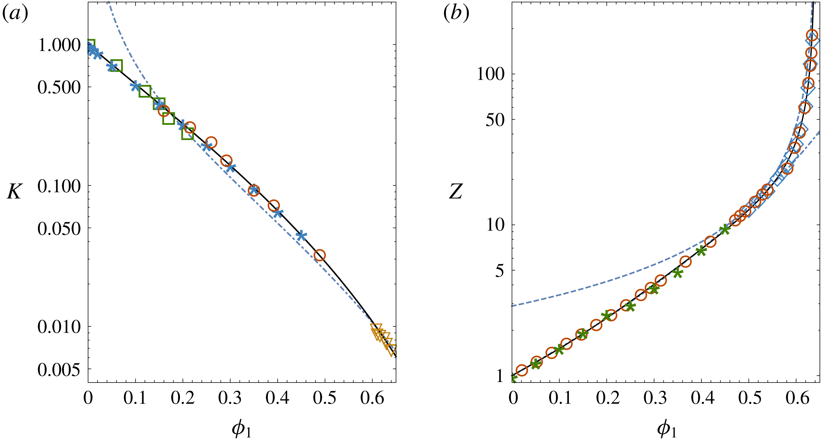
yields a good fit to data and gives similar predictions to the Kozeny–Carman equation near close packing (figure 2
a). For spherical particles the Kozeny–Carman equation is
 $k=R_{1}^{2}(1-\unicode[STIX]{x1D719}_{1})^{3}/45\unicode[STIX]{x1D719}_{1}^{2}$
(Carman Reference Carman1939), so that (4.1) gives
 $$\begin{eqnarray}K=\frac{(1-\unicode[STIX]{x1D719}_{1})^{3}}{10\unicode[STIX]{x1D719}_{1}}\end{eqnarray}$$
as the Kozeny–Carman sedimentation coefficient (Philipse & Pathmamanoharan Reference Philipse and Pathmamanoharan1993). Equation (4.3) is plotted in figure 2(a) as the dash-dot curve.
Plots of (a) the mobility function
 $K(\unicode[STIX]{x1D719}_{1})$
and (b) the compressibility factor
 $Z(\unicode[STIX]{x1D719}_{1}).$
In (a) the data are from the sedimentation experiments of Xue et al. (Reference Xue, Herbolzheimer, Rutgers, Russel and Chaikin1992) (circles) and Buzzaccaro et al. (Reference Buzzaccaro, Tripodi, Rusconi, Vigolo and Piazza2008) (squares); from the numerical simulations of (Ladd Reference Ladd1990) (stars); and from the permeation experiments of Carman (Reference Carman1939) (triangles). The curves in (a) are from (4.2) (solid) and from the Kozeny–Carman equation (4.3) (dash-dot). In (b) the data are from the sedimentation experiments of Buzzaccaro, Rusconi & Piazza (Reference Buzzaccaro, Rusconi and Piazza2007) (stars) and the molecular dynamics simulations of Wu & Sadus (Reference Wu and Sadus2005) (circles) and Rintoul & Torquato (Reference Rintoul and Torquato1996) (diamonds). The curves are from (4.6) (solid), from the Carnahan–Starling equation of state (4.5) (dash-dot) and the Woodcock equation of state
 $Z=1.85/(\unicode[STIX]{x1D719}_{p}-\unicode[STIX]{x1D719}_{1})$
(dash).

4.2 Osmotic pressures
4.2.1 Host particles
Similarly to
 $k$
, in the dilute tracer limit
 $\unicode[STIX]{x1D719}_{2}\rightarrow 0$
, the host osmotic pressure
 $\unicode[STIX]{x1D6F1}$
depends only on
 $\unicode[STIX]{x1D719}_{1}$
(Lekkerkerker & Stroobants Reference Lekkerkerker and Stroobants1993). The osmotic pressure can then be written as
 $$\begin{eqnarray}\unicode[STIX]{x1D6F1}=n_{1}k_{B}TZ,\end{eqnarray}$$
where
 $Z(\unicode[STIX]{x1D719}_{1})$
is the hard-sphere compressibility factor (Russel et al.
Reference Russel, Seville and Schowalter1989). Over the range
 $(0<\unicode[STIX]{x1D719}_{1}<0.55)$
,
 $Z$
is given by the Carnahan–Starling equation
 $$\begin{eqnarray}Z=\frac{1+\unicode[STIX]{x1D719}_{1}+\unicode[STIX]{x1D719}_{1}^{2}-\unicode[STIX]{x1D719}_{1}^{3}}{(1-\unicode[STIX]{x1D719}_{1})^{3}}\end{eqnarray}$$
(Carnahan & Starling Reference Carnahan and Starling1969), while at higher volume fractions
 $Z$
diverges according to Woodcock’s equation
 $Z\sim (\unicode[STIX]{x1D719}_{p}-\unicode[STIX]{x1D719}_{1})^{-1}$
, where
 $\unicode[STIX]{x1D719}_{p}=0.64$
is the volume fraction at random close packing (Woodcock Reference Woodcock1981; Russel et al.
Reference Russel, Seville and Schowalter1989; O’Hern et al.
Reference O’Hern, Silbert, Liu and Nagel2003). The following empirical expression,
 $$\begin{eqnarray}Z(\unicode[STIX]{x1D719}_{1})=\frac{1+(4-1/\unicode[STIX]{x1D719}_{p})\unicode[STIX]{x1D719}_{1}+32\unicode[STIX]{x1D719}_{1}^{3}-55\unicode[STIX]{x1D719}_{1}^{4}}{1-\unicode[STIX]{x1D719}_{1}/\unicode[STIX]{x1D719}_{p}},\end{eqnarray}$$
agrees with the Carnahan–Starling equation as
 $\unicode[STIX]{x1D719}_{1}\rightarrow 0$
and with the Woodcock equation as
 $\unicode[STIX]{x1D719}_{1}\rightarrow \unicode[STIX]{x1D719}_{p}$
. Equation (4.6) is plotted in figure 2(b) along with data from sedimentation experiments (Buzzaccaro et al.
Reference Buzzaccaro, Rusconi and Piazza2007) and molecular dynamics simulations (Rintoul & Torquato Reference Rintoul and Torquato1996; Wu & Sadus Reference Wu and Sadus2005). Differentiating (4.4) with respect to
 $n_{i}$
gives
 $$\begin{eqnarray}\unicode[STIX]{x1D6F1}_{1}=k_{B}T\frac{\text{d}(\unicode[STIX]{x1D719}_{1}Z)}{\text{d}\unicode[STIX]{x1D719}_{1}}\quad \text{and}\quad \unicode[STIX]{x1D6F1}_{2}=0.\end{eqnarray}$$
4.2.2 Tracer particles
Assuming the tracer concentration in the reservoir compartment B is dilute the osmotic pressure
 $\unicode[STIX]{x03C0}$
is
 $$\begin{eqnarray}\unicode[STIX]{x03C0}=n_{r}k_{B}T.\end{eqnarray}$$
Differentiating
 $\unicode[STIX]{x03C0}$
with respect to
 $n_{i}$
gives, bearing in mind that
 $n_{r}=n_{2}/\unicode[STIX]{x1D6FC}$
and assuming
 $\unicode[STIX]{x1D6FC}=\unicode[STIX]{x1D6FC}(n_{1})$
(Lekkerkerker & Stroobants Reference Lekkerkerker and Stroobants1993),
 $$\begin{eqnarray}\unicode[STIX]{x03C0}_{1}=-\frac{n_{2}\unicode[STIX]{x1D6FC}_{1}\unicode[STIX]{x03C0}_{r}}{\unicode[STIX]{x1D6FC}^{2}}\quad \text{and}\quad \unicode[STIX]{x03C0}_{2}=\frac{\unicode[STIX]{x03C0}_{r}}{\unicode[STIX]{x1D6FC}},\end{eqnarray}$$
where
 $\unicode[STIX]{x1D6FC}_{1}=(\unicode[STIX]{x2202}\unicode[STIX]{x1D6FC}/\unicode[STIX]{x2202}n_{1})_{T,P,n_{2}}$
and
 $\unicode[STIX]{x03C0}_{r}=(\unicode[STIX]{x2202}\unicode[STIX]{x03C0}/\unicode[STIX]{x2202}n_{r})_{T,p}=k_{B}T.$
4.3 Equilibrium partition coefficient
The partition coefficient
 $\unicode[STIX]{x1D6FC}$
can be obtained by equating the chemical potential of the tracer particles in the suspension and reservoir of figure 1. In the dilute limit
 $(\unicode[STIX]{x1D719}_{2}\ll \unicode[STIX]{x1D719}_{1}\ll 1)$
, equation (2.7b
) gives the chemical potential of the tracer particles in the suspension (compartment A) as
 $$\begin{eqnarray}\unicode[STIX]{x1D707}_{2}=\unicode[STIX]{x1D707}_{2}^{0}+k_{B}T(\ln \unicode[STIX]{x1D719}_{2}+b_{12}\unicode[STIX]{x1D719}_{1}).\end{eqnarray}$$
In the limit
 $\unicode[STIX]{x1D719}_{r}\ll 1$
the chemical potential of the tracer particles in the reservoir is
 $$\begin{eqnarray}\unicode[STIX]{x1D707}_{r}=\unicode[STIX]{x1D707}_{2}^{0}+k_{B}T\ln \unicode[STIX]{x1D719}_{r},\end{eqnarray}$$
where
 $\unicode[STIX]{x1D719}_{r}=v_{2}n_{r}$
is the tracer volume fraction in the reservoir. Equating the chemical potentials at equilibrium,
 $\unicode[STIX]{x1D707}_{2}=\unicode[STIX]{x1D707}_{r},$
gives the partition coefficient as
 $$\begin{eqnarray}\unicode[STIX]{x1D6FC}=\frac{\unicode[STIX]{x1D719}_{2}}{\unicode[STIX]{x1D719}_{r}}=\text{e}^{-b_{12}\unicode[STIX]{x1D719}_{1}}.\end{eqnarray}$$
As
 $\unicode[STIX]{x1D719}_{1}\rightarrow 0$
, (4.12) becomes
 $$\begin{eqnarray}\unicode[STIX]{x1D6FC}=1-b_{12}\unicode[STIX]{x1D719}_{1}=1-v_{ex}n_{1},\end{eqnarray}$$
where
 $v_{ex}=b_{12}v_{1}=(4/3)\unicode[STIX]{x03C0}(R_{1}+R_{2})^{3}$
is the volume excluded to the centre of a tracer particle by a host particle. Thus in the dilute limit
 $\unicode[STIX]{x1D6FC}$
is a measure of the free volume fraction available to the tracer particles (Lekkerkerker & Stroobants Reference Lekkerkerker and Stroobants1993; Annunziata Reference Annunziata2008). When
 $R_{2}\ll R_{1}$
,
 $\unicode[STIX]{x1D6FC}$
is equal to the void fraction
 $1-\unicode[STIX]{x1D719}_{1}$
.
4.4 Preferential interaction coefficient
The preferential interaction coefficient appearing in (3.11c ) is
 $$\begin{eqnarray}\unicode[STIX]{x1D6FE}=-\frac{\unicode[STIX]{x1D707}_{21}}{\unicode[STIX]{x1D707}_{22}}=-\frac{\unicode[STIX]{x03C0}_{1}}{\unicode[STIX]{x03C0}_{2}}=\left(\frac{\unicode[STIX]{x2202}n_{2}}{\unicode[STIX]{x2202}n_{1}}\right)_{T,P,\unicode[STIX]{x03C0}},\end{eqnarray}$$
and measures the number of tracer particles that must be added to compartment A of figure 1 per added host particle, in order to maintain
 $\unicode[STIX]{x03C0}(n_{r})$
constant in compartment B. For charged proteins and adsorbing colloids,
 $\unicode[STIX]{x1D6FE}$
can be positive or negative (Schneider & Trout Reference Schneider and Trout2009); for hard-sphere systems involving only volume exclusion
 $\unicode[STIX]{x1D6FE}$
is negative (the host particles exclude tracer particles). With (4.9) and (4.12) the preferential interaction coefficient
 $\unicode[STIX]{x1D6FE}$
is
 $$\begin{eqnarray}\unicode[STIX]{x1D6FE}=n_{2}\frac{\unicode[STIX]{x1D6FC}_{1}}{\unicode[STIX]{x1D6FC}}=-n_{2}v_{1}b_{12}=-n_{2}v_{ex}.\end{eqnarray}$$
Thus, for each additional host particle added to compartment A of figure 1,
 $n_{2}v_{ex}$
tracer particles must be removed in the dilute limit to maintain osmotic equilibrium with compartment B.
4.5 Tortuosity and reflection coefficient
4.5.1 Definition and dilute limit
The diffusive tortuosity factor
 $\unicode[STIX]{x1D70F}$
is defined as the ratio of the tracer diffusivity
 $D_{t}$
in the suspension to the Stokes–Einstein diffusivity
 $D_{2}^{0}=k_{B}T/6\unicode[STIX]{x03C0}R_{2}\unicode[STIX]{x1D702}_{0}$
of a tracer particle in the pure suspending fluid:
 $$\begin{eqnarray}\unicode[STIX]{x1D70F}\equiv D_{t}/D_{2}^{0}.\end{eqnarray}$$
In the dilute limit an expression for
 $\unicode[STIX]{x1D70F}$
can be obtained using Batchelor’s equations (2.6). Equation (3.10c
) combined with (2.6) and (4.8) gives in the limit
 $\unicode[STIX]{x1D719}_{2}\ll \unicode[STIX]{x1D719}_{1}\ll 1$
 $$\begin{eqnarray}\unicode[STIX]{x1D70F}=1-\unicode[STIX]{x1D70F}_{1}\unicode[STIX]{x1D719}_{1},\end{eqnarray}$$
where
 $\unicode[STIX]{x1D70F}_{1}=-K_{21}^{\prime }=2.5\unicode[STIX]{x1D706}_{12}/(\unicode[STIX]{x1D706}_{12}+0.22)$
. Similarly, equation (3.10b
) can be combined with (4.13) and (2.6a,b
) in the limit
 $\unicode[STIX]{x1D719}_{2}\ll \unicode[STIX]{x1D719}_{1}\ll 1$
to obtain
 $$\begin{eqnarray}\unicode[STIX]{x1D70E}=\unicode[STIX]{x1D70E}_{1}\unicode[STIX]{x1D719}_{1},\end{eqnarray}$$
where
 $\unicode[STIX]{x1D70E}_{1}=b_{12}+K_{12}^{\prime \prime }$
. Equation (4.18) shows that, because of excluded volume and long-range viscous effects, the host particles have a ‘membrane separation’ effect (
 $\unicode[STIX]{x1D70E}>0$
) on the tracer particles even in the dilute limit. Only when the tracer particles have negligible volume (
 $\unicode[STIX]{x1D706}_{12}=R_{2}/R_{1}\rightarrow 0$
) does
 $\unicode[STIX]{x1D70E}$
reduce to zero. In concentrated systems,
 $\unicode[STIX]{x1D70F}(\unicode[STIX]{x1D719}_{1})$
and
 $\unicode[STIX]{x1D70E}(\unicode[STIX]{x1D719}_{1})$
can be obtained using results of hindered diffusion models of tracer particles in cylindrical pores, as detailed below.
4.5.2 Cylindrical pores
Expressions for
 $\unicode[STIX]{x1D70F}$
and
 $\unicode[STIX]{x1D70E}$
of spherical tracer particles in cylindrical pores have been derived by Anderson & Quinn (Reference Anderson and Quinn1974) in the form
 $$\begin{eqnarray}\unicode[STIX]{x1D70F}=(1-\unicode[STIX]{x1D706}_{p})^{2}K_{d},\end{eqnarray}$$
and
 $$\begin{eqnarray}\unicode[STIX]{x1D70E}=1-(1-\unicode[STIX]{x1D706}_{p})^{2}K_{c},\end{eqnarray}$$
where
 $K_{c}(\unicode[STIX]{x1D706}_{p})$
and
 $K_{d}(\unicode[STIX]{x1D706}_{p})$
are hydrodynamic factors and
 $\unicode[STIX]{x1D706}_{p}=R_{2}/R_{p}$
is the ratio of the tracer particle radius
 $R_{2}$
to the pore radius
 $R_{p}$
. Equations (4.20) and (4.19) assume the tracer particles are equal to or smaller than the pore radius (
 $\unicode[STIX]{x1D706}_{p}\leqslant 1$
). When
 $\unicode[STIX]{x1D706}_{p}>1$
,
 $\unicode[STIX]{x1D70E}=1$
and
 $\unicode[STIX]{x1D70F}=0$
since the tracer particles in this case cannot enter the pores.
For
 $\unicode[STIX]{x1D706}_{p}\leqslant 0.4$
, Anderson & Quinn (Reference Anderson and Quinn1974) obtained
 $K_{c}=(1+2\unicode[STIX]{x1D706}_{p}-\unicode[STIX]{x1D706}_{p}^{2})(1-(2/3)\unicode[STIX]{x1D706}_{p}^{2}-0.163\unicode[STIX]{x1D706}_{p}^{3})$
and
 $K_{d}=1-2.1\unicode[STIX]{x1D706}_{p}+2.09\unicode[STIX]{x1D706}_{p}^{3}-0.95\unicode[STIX]{x1D706}_{p}^{5}$
. Recent finite element simulations (Oatley-Radcliffe et al.
Reference Oatley-Radcliffe, Williams, Ainscough, Lee, Johnson and Williams2015), valid over the range
 $0\leqslant \unicode[STIX]{x1D706}_{p}\leqslant 0.98$
, can be fit by the empirical equations
 $$\begin{eqnarray}K_{c}=(1+2\unicode[STIX]{x1D706}_{p}-\unicode[STIX]{x1D706}_{p}^{2})(1-0.81\unicode[STIX]{x1D706}_{p}^{2}+0.31\unicode[STIX]{x1D706}_{p}^{3})\end{eqnarray}$$
and
 $$\begin{eqnarray}K_{d}=(1-\unicode[STIX]{x1D706}_{p})^{2.2+0.55\unicode[STIX]{x1D706}_{p}},\end{eqnarray}$$
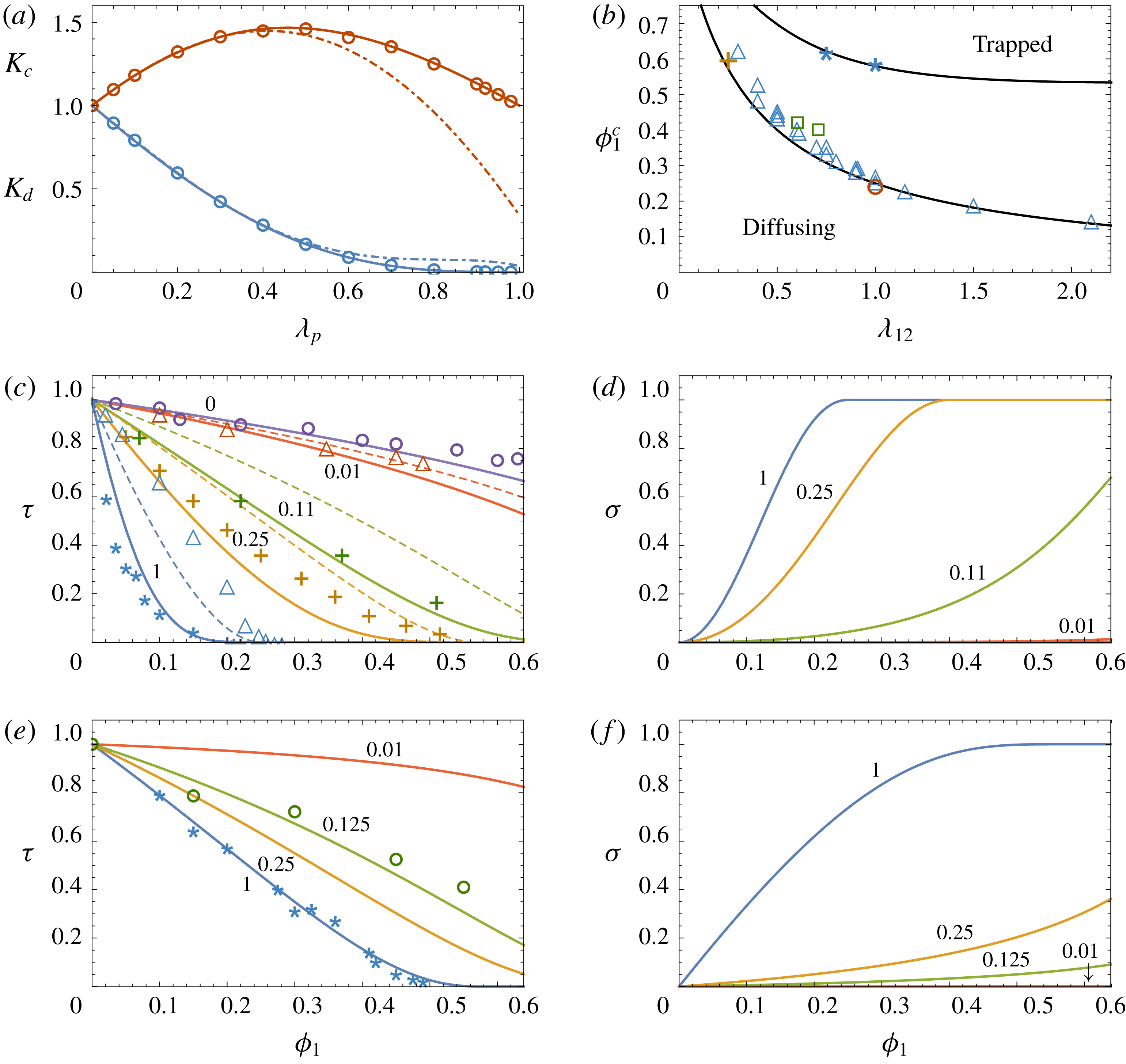
as shown in figure 3(a).
(a) Convective and diffusive hydrodynamic factors
 $K_{c}$
(upper curve) and
 $K_{d}$
(lower curve) plotted versus the tracer/cylindrical-pore size ratio
 $\unicode[STIX]{x1D706}_{p}=R_{2}/R_{p}$
. The circles are data from finite element simulations (Oatley-Radcliffe et al.
Reference Oatley-Radcliffe, Williams, Ainscough, Lee, Johnson and Williams2015); the dash-dot curves are from the theory of Anderson & Quinn (Reference Anderson and Quinn1974) (valid for
 $\unicode[STIX]{x1D706}_{p}\leqslant 0.4$
); and the solid curves are from (4.21) and (4.22). (b) Glass transition volume fraction
 $\unicode[STIX]{x1D719}_{1}^{c}(\unicode[STIX]{x1D706}_{12})$
for tracer particles in porous media (lower curve) and suspensions (upper curve), plotted versus the tracer/host-particle size ratio
 $\unicode[STIX]{x1D706}_{12}=R_{2}/R_{1}$
. The data are from Kim & Torquato (Reference Kim and Torquato1992) (crosses), Gimel & Taco (Reference Gimel and Taco2011) (triangles), Sung & Yethiraj (Reference Sung and Yethiraj2008) (circles), Lockett & Al-Habbooby (Reference Lockett and Al-Habbooby1974) (squares) and Zaccarelli, Liddle & Poon (Reference Zaccarelli, Liddle and Poon2015) (stars). (c) Porous media tortuosity factor
 $\unicode[STIX]{x1D70F}(\unicode[STIX]{x1D719}_{1})$
calculated from (4.25) for different values of
 $\unicode[STIX]{x1D706}_{12}$
. The dashed curves are from (4.25) with
 $K_{d}=1$
. The data are from Neale & Nader (Reference Neale and Nader1973) (circles), Kim & Torquato (Reference Kim and Torquato1992) (crosses), Sung & Yethiraj (Reference Sung and Yethiraj2008) (stars) and Gimel & Taco (Reference Gimel and Taco2011) (triangles). (d) Porous media reflection coefficient
 $\unicode[STIX]{x1D70E}(\unicode[STIX]{x1D719}_{1})$
for the same size ratios as in figure (c), calculated from (4.26). (e) Suspension tortuosity factor
 $\unicode[STIX]{x1D70F}(\unicode[STIX]{x1D719}_{1})$
calculated from (4.28) for several values of
 $\unicode[STIX]{x1D706}_{12}$
, with data from Segrè et al. (Reference Segrè, Meeker, Pusey and Poon1995) (stars) and Guan et al. (Reference Guan, Wang and Granick2014) (circles). (f) Suspension reflection coefficient
 $\unicode[STIX]{x1D70E}(\unicode[STIX]{x1D719}_{1})$
for the same size ratios as in figure (e), calculated from (4.29). The numbers next to the curves in (c–f) are the values of
 $\unicode[STIX]{x1D706}_{12}$
.

4.5.3 Porous media
Equations (4.20)–(4.22) can be applied to porous media by noting that the approximate physical pore radius is
 $R_{p}=\unicode[STIX]{x1D716}/S_{p}(1-\unicode[STIX]{x1D716}),$
where
 $\unicode[STIX]{x1D716}=1-\unicode[STIX]{x1D719}_{1}$
is the void fraction and
 $S_{p}$
is the specific surface area of the porous matrix (Carman Reference Carman1939). For a matrix composed of spherical particles
 $S_{p}=4\unicode[STIX]{x03C0}R_{1}^{2}/(4/3)\unicode[STIX]{x03C0}R_{1}^{3}=3/R_{1}$
(Bird, Stuart & Lightfoot Reference Bird, Stuart and Lightfoot2002), giving
 $$\begin{eqnarray}\unicode[STIX]{x1D706}_{p}=\frac{R_{2}}{R_{p}}=\frac{3\unicode[STIX]{x1D706}_{12}\unicode[STIX]{x1D719}_{1}}{(1-\unicode[STIX]{x1D719}_{1})}.\end{eqnarray}$$
In porous media there is in addition a geometric tortuosity
 $\unicode[STIX]{x1D70F}_{g}$
related to the increased length of the meandering pathways tracer particles take through the pore space relative to straight cylindrical pores (Malusis, Shackelford & Maneval Reference Malusis, Shackelford and Maneval2012; Ghanbarian et al.
Reference Ghanbarian, Hunt, Ewing and Sahimi2013). For spherical matrix particles Delgado (Reference Delgado2006) obtains
 $$\begin{eqnarray}\unicode[STIX]{x1D70F}_{g}=(1-\unicode[STIX]{x1D719}_{1})^{0.4}.\end{eqnarray}$$
The tortuosity and reflection coefficient can then be written as
 $$\begin{eqnarray}\unicode[STIX]{x1D70F}=\left\{\begin{array}{@{}ll@{}}\unicode[STIX]{x1D70F}_{g}(1-\unicode[STIX]{x1D706}_{p})^{2}K_{d}(\unicode[STIX]{x1D706}_{p})\quad & \text{if }0\leqslant \unicode[STIX]{x1D706}_{p}\leqslant 1,\\ 1\quad & \text{if }\unicode[STIX]{x1D706}_{p}>1\end{array}\right.\end{eqnarray}$$
and
 $$\begin{eqnarray}\unicode[STIX]{x1D70E}=\left\{\begin{array}{@{}ll@{}}1-(1-\unicode[STIX]{x1D706}_{p})^{2}K_{c}(\unicode[STIX]{x1D706}_{p})\quad & \text{if }0\leqslant \unicode[STIX]{x1D706}_{p}\leqslant 1,\\ 1\quad & \text{if }\unicode[STIX]{x1D706}_{p}>1.\end{array}\right.\end{eqnarray}$$
Figure 3(c,d) shows
 $\unicode[STIX]{x1D70F}$
and
 $\unicode[STIX]{x1D70E}$
plotted versus
 $\unicode[STIX]{x1D719}_{1}$
for several values of
 $\unicode[STIX]{x1D706}_{12},$
along with experimental data for
 $\unicode[STIX]{x1D70F}$
from Neale & Nader (Reference Neale and Nader1973) and numerical data from Kim & Torquato (Reference Kim and Torquato1992), Sung & Yethiraj (Reference Sung and Yethiraj2008) and Gimel & Taco (Reference Gimel and Taco2011). As the numerical simulations did not include viscous effects, also shown in figure 3(c) are results from (4.25) with the hydrodynamic factor
 $K_{d}$
set to 1 (dashed curves).
In the dilute host limit (
 $\unicode[STIX]{x1D719}_{1}\ll 1$
), the pore size is large (
 $R_{p}\gg R_{2}$
) and the host particles have little effect on the tracer diffusion, so that
 $\unicode[STIX]{x1D70F}\rightarrow 1$
and
 $\unicode[STIX]{x1D70E}\rightarrow 0$
. At higher matrix concentrations the pore radius
 $R_{p}$
approaches the tracer radius
 $R_{2}$
and the tracer diffusion is strongly hindered (
 $\unicode[STIX]{x1D70F}<1$
). At a critical host volume fraction
 $\unicode[STIX]{x1D719}_{1}^{c}$
,
 $R_{p}=R_{2}$
and the particles are trapped within the pores, so that
 $\unicode[STIX]{x1D70F}=0$
and
 $\unicode[STIX]{x1D70E}=1$
;
 $\unicode[STIX]{x1D719}_{1}^{c}$
represents the glass transition of the tracer particles within the host matrix (Voigtmann Reference Voigtmann2011). Setting
 $\unicode[STIX]{x1D706}_{p}=1$
in (4.23) gives
 $$\begin{eqnarray}\unicode[STIX]{x1D719}_{1}^{c}=(1+3\unicode[STIX]{x1D706}_{12})^{-1},\end{eqnarray}$$
so that
 $\unicode[STIX]{x1D719}_{1}^{c}=0.25$
when
 $\unicode[STIX]{x1D706}_{12}=1$
. Figure 3(b) (lower curve) shows
 $\unicode[STIX]{x1D719}_{1}^{c}$
plotted versus
 $\unicode[STIX]{x1D706}_{12}$
along with experimental and numerical data from Kim & Torquato (Reference Kim and Torquato1992), Sung & Yethiraj (Reference Sung and Yethiraj2008) and Gimel & Taco (Reference Gimel and Taco2011). In the case of very small tracer particles (
 $\unicode[STIX]{x1D706}_{12}\leqslant 0.11$
in figure 3
c) the particles are hindered by the host matrix as
 $\unicode[STIX]{x1D719}_{1}$
increases, but can still diffuse throughout the pore space even up to the close-packed limit
 $\unicode[STIX]{x1D719}_{p}=0.64$
and no tracer glass transition occurs.
4.5.4 Suspensions
In contrast to porous media where the host matrix is fixed in place, in suspensions the host particles are able to move in response to viscous and Brownian forces (Bruna & Chapman Reference Bruna and Chapman2015; Wang & Brady Reference Wang and Brady2015; Sentjabrskaja et al.
Reference Sentjabrskaja, Zaccarelli, Michele, De Sciortino, Tartaglia, Voigtmann, Egelhaaf and Laurati2016). Tracer particles in suspensions therefore can diffuse even when the tracer radius
 $R_{2}$
is larger than the pore size
 $R_{p}$
; the host particles adjust their positions, opening dynamic heterogeneities through which the tracer particles can pass (Rallison Reference Rallison1988; Kumar, Szamel & Douglas Reference Kumar, Szamel and Douglas2006; Wang et al.
Reference Wang, Kuo, Bae and Granick2012; Guan et al.
Reference Guan, Wang and Granick2014). Previously, this effect has been modelled phenomenologically by assuming the host suspension is composed of fast and slow domains having different viscosities (Hodgdon & Stillinger Reference Hodgdon and Stillinger1993; Xia & Wolynes Reference Xia and Wolynes2001; Fan, Dhont & Tuinier Reference Fan, Dhont and Tuinier2007) or by introducing a scaling factor for the tracer radius (Kalwarczyk et al.
Reference Kalwarczyk, Sozanski, Jakiela, Wisniewska, Kalwarczyk, Kryszczuk, Hou and Holyst2014). A similar method used here is to assume the tracer particles in suspensions experience an effective diffusive pore size
 $R_{d}=c_{d}R_{p}$
, where
 $c_{d}>1$
is an empirical scaling factor to be determined.
Related to this issue is the fact that long range viscous interactions in suspensions are different from porous media (Hinch Reference Hinch1977; Ladd Reference Ladd1990; Koch, Hill & Sangani Reference Koch, Hill and Sangani1998), and therefore the porous medium hydrodynamic factors
 $K_{d}$
and
 $K_{c}$
cannot be used for suspensions. An alternative approach is to use (4.17) and (4.18) obtained from Batchelor’s suspension results, and assume power laws for
 $\unicode[STIX]{x1D70F}$
and
 $\unicode[STIX]{x1D70E}$
of the form
 $$\begin{eqnarray}\unicode[STIX]{x1D70F}=\left\{\begin{array}{@{}ll@{}}(1-\unicode[STIX]{x1D706}_{d})^{a_{\unicode[STIX]{x1D70F}}}\quad & \text{if }0\leqslant \unicode[STIX]{x1D706}_{d}\leqslant 1,\\ 1\quad & \text{if }\unicode[STIX]{x1D706}_{d}>1\end{array}\right.\end{eqnarray}$$
and
 $$\begin{eqnarray}\unicode[STIX]{x1D70E}=\left\{\begin{array}{@{}ll@{}}1-(1-\unicode[STIX]{x1D706}_{d})^{a_{\unicode[STIX]{x1D70E}}}\quad & \text{if }0\leqslant \unicode[STIX]{x1D706}_{d}\leqslant 1,\\ 1\quad & \text{if }\unicode[STIX]{x1D706}_{d}>1,\end{array}\right.\end{eqnarray}$$
where
 $$\begin{eqnarray}\unicode[STIX]{x1D706}_{d}=\frac{R_{2}}{R_{d}}=\frac{3\unicode[STIX]{x1D706}_{12}\unicode[STIX]{x1D719}_{1}}{c_{d}(1-\unicode[STIX]{x1D719}_{1})}.\end{eqnarray}$$
The exponents
 $a_{\unicode[STIX]{x1D70F}}$
and
 $a_{\unicode[STIX]{x1D70E}}$
can be obtained by requiring (4.28) and (4.29) to match (4.17) and (4.18) in the limit
 $\unicode[STIX]{x1D719}_{1}\rightarrow 0$
. In this limit (4.28) and (4.29) become
 $\unicode[STIX]{x1D70F}=1-3\unicode[STIX]{x1D706}_{12}a_{\unicode[STIX]{x1D70F}}\unicode[STIX]{x1D719}_{1}/c_{d}$
and
 $\unicode[STIX]{x1D70E}=3\unicode[STIX]{x1D706}_{12}a_{\unicode[STIX]{x1D70E}}\unicode[STIX]{x1D719}_{1}/c_{d}$
giving
 $$\begin{eqnarray}a_{\unicode[STIX]{x1D70F}}=\frac{\unicode[STIX]{x1D70F}_{1}c_{d}}{3\unicode[STIX]{x1D706}_{12}}\quad \text{and}\quad a_{\unicode[STIX]{x1D70E}}=\frac{\unicode[STIX]{x1D70E}_{1}c_{d}}{3\unicode[STIX]{x1D706}_{12}}.\end{eqnarray}$$
A fit of (4.28) to data for the viscosity of a hard-sphere suspension (§ 6.1) gives
 $$\begin{eqnarray}c_{d}=3\frac{\unicode[STIX]{x1D719}_{g}}{(1-\unicode[STIX]{x1D719}_{g})}\frac{(1+\unicode[STIX]{x1D706}_{12}^{2})}{(1+\unicode[STIX]{x1D706}_{12})},\end{eqnarray}$$
where
 $\unicode[STIX]{x1D719}_{g}=0.58$
is the volume fraction at the hard-sphere glass transition (Hunter & Weeks Reference Hunter and Weeks2012).
The tortuosity
 $\unicode[STIX]{x1D70F}(\unicode[STIX]{x1D719}_{1})$
and reflection coefficient
 $\unicode[STIX]{x1D70E}(\unicode[STIX]{x1D719}_{1})$
calculated from (4.28)–(4.32) are plotted in figure 3(e,f) for several values of the particle size ratio
 $\unicode[STIX]{x1D706}_{12}=R_{2}/R_{1}$
, along with experimental data from Segrè et al. (Reference Segrè, Meeker, Pusey and Poon1995) and Guan et al. (Reference Guan, Wang and Granick2014). The tracer glass transition
 $\unicode[STIX]{x1D719}_{1}^{c}$
at which
 $\unicode[STIX]{x1D70F}=0$
in suspensions can be obtained by setting
 $\unicode[STIX]{x1D706}_{d}=1$
in (4.30) giving
 $$\begin{eqnarray}\unicode[STIX]{x1D719}_{1}^{c}=(1+3\unicode[STIX]{x1D706}_{12}/c_{d})^{-1}.\end{eqnarray}$$
Equation (4.33) is plotted as the upper curve in figure 3(b), along with estimates of
 $\unicode[STIX]{x1D719}_{1}^{c}$
from the data of Zaccarelli et al. (Reference Zaccarelli, Liddle and Poon2015). In suspensions the tracer diffusion is significantly less hindered than in porous media. In the self-diffusion case (
 $\unicode[STIX]{x1D706}_{12}=1$
) tracer diffusion in suspensions ceases at the host-matrix glass transition
 $\unicode[STIX]{x1D719}_{1}^{c}=\unicode[STIX]{x1D719}_{g}=0.58$
, while for porous media the tracer glass transition occurs much earlier at
 $\unicode[STIX]{x1D719}_{1}^{c}=0.25$
.
4.6 Cross-diffusion factor
The cross-diffusion factor in (3.11c ) is
 $$\begin{eqnarray}\ell =\left(\frac{\unicode[STIX]{x1D70E}+\unicode[STIX]{x1D6FC}-1}{\unicode[STIX]{x1D6FC}}\right)=\frac{n_{1}}{n_{2}}\frac{\unicode[STIX]{x1D613}_{12}}{\unicode[STIX]{x1D613}_{11}},\end{eqnarray}$$
and is a measure of fluid-mediated friction interactions between the tracer and host particles. In the dilute limit
 $(\unicode[STIX]{x1D719}_{2}\ll \unicode[STIX]{x1D719}_{1}\ll 1),$
inserting (4.13) and (4.18) into (4.34) gives
 $$\begin{eqnarray}\ell =K_{12}^{\prime \prime }\unicode[STIX]{x1D719}_{1}.\end{eqnarray}$$
At higher host volume fractions
 $\ell$
can be obtained using (4.29) for
 $\unicode[STIX]{x1D70E}(\unicode[STIX]{x1D719}_{1})$
and (4.12) for
 $\unicode[STIX]{x1D6FC}(\unicode[STIX]{x1D719}_{1})$
. At host volume fractions above the trapping concentration
 $\unicode[STIX]{x1D719}_{1}^{c}$
where
 $\unicode[STIX]{x1D70E}=1$
, equation (4.34) gives
 $\ell =1.$
5 Diffusion and cross-diffusion coefficients
With the results of § 4, equations (3.11) can be used to calculate the diffusion coefficients
 $D_{ij}$
as functions of
 $\unicode[STIX]{x1D719}_{1}$
. In terms of dimensionless quantities equations (3.11) can be written as
 $$\begin{eqnarray}\hat{D}_{11}=K(\hat{\unicode[STIX]{x1D6F1}}_{1}+\unicode[STIX]{x1D70E}\hat{\unicode[STIX]{x03C0}}_{1}),\quad \hat{D}_{12}=K(\hat{\unicode[STIX]{x1D6F1}}_{2}+\unicode[STIX]{x1D70E}\hat{\unicode[STIX]{x03C0}}_{2}),\end{eqnarray}$$
 $$\begin{eqnarray}\hat{D}_{21}=\hat{\ell }\hat{D}_{11}-\unicode[STIX]{x1D6FE}\unicode[STIX]{x1D70F},\quad \hat{D}_{22}=\hat{\ell }\hat{D}_{12}+\unicode[STIX]{x1D70F},\end{eqnarray}$$
where
 $\hat{D}_{ij}=D_{ij}/D_{i}^{0}$
,
 $\hat{\unicode[STIX]{x1D6F1}}_{i}=\unicode[STIX]{x1D6F1}_{i}/k_{B}T$
,
 $\hat{\unicode[STIX]{x03C0}}_{i}=\unicode[STIX]{x03C0}_{i}/k_{B}T$
and
 $\hat{\ell }=\unicode[STIX]{x1D719}_{2}\ell /\unicode[STIX]{x1D719}_{1}\unicode[STIX]{x1D706}_{12}^{2}$
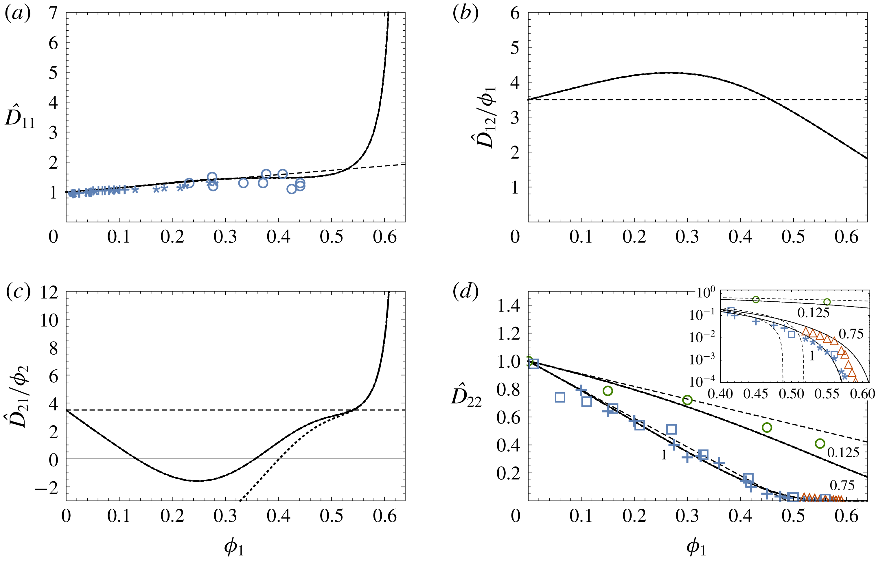
. The
 $\hat{D}_{ij}$
are plotted in figure 4 as functions of
 $\unicode[STIX]{x1D719}_{1}$
for the case
 $\unicode[STIX]{x1D719}_{2}=10^{-5}$
and
 $\unicode[STIX]{x1D706}_{12}=1$
, along with experimental data and Batchelor’s equations (2.9) (dashed lines). When the tracer particles are sufficiently dilute that
 $\unicode[STIX]{x1D719}_{2}\ll \unicode[STIX]{x1D6FC}$
(corresponding via (4.12) to
 $\unicode[STIX]{x1D719}_{r}\ll 1$
), then several terms involving
 $\unicode[STIX]{x1D719}_{2}$
in (3.11) can be neglected, yielding the simpler equations
 $$\begin{eqnarray}\hat{D}_{11}=K\hat{\unicode[STIX]{x1D6F1}}_{1},\quad \hat{D}_{12}=K\unicode[STIX]{x1D70E}\hat{\unicode[STIX]{x03C0}}_{2},\end{eqnarray}$$
 $$\begin{eqnarray}\hat{D}_{21}=\hat{\ell }\hat{D}_{11}-\unicode[STIX]{x1D6FE}\unicode[STIX]{x1D70F},\quad \hat{D}_{22}=\unicode[STIX]{x1D70F}.\end{eqnarray}$$
Equations (5.2) are plotted in figure 4 as the dash-dot curves; for the case
 $\unicode[STIX]{x1D719}_{2}=10^{-5}$
they are nearly indistinguishable from the solid curves. If in addition
 $\unicode[STIX]{x1D70F}\ll 1$
(crowded host matrix), then the
 $\unicode[STIX]{x1D6FE}\unicode[STIX]{x1D70F}$
term in (5.2c
) can also be neglected, so that
 $$\begin{eqnarray}\hat{D}_{21}=\hat{\ell }\hat{D}_{11}.\end{eqnarray}$$
Equation (5.3) is plotted in figure 4(c) as the dotted curve, which agrees with (5.2c
) when
 $\unicode[STIX]{x1D719}_{1}\gtrsim 0.5$
.
Plots of the dimensionless diffusion and cross-diffusion coefficients calculated from (5.1) as functions of
 $\unicode[STIX]{x1D719}_{1}$
for
 $\unicode[STIX]{x1D719}_{2}=10^{-5}$
and
 $\unicode[STIX]{x1D706}_{12}=1$
: (a) host particle Fickian diffusion coefficient
 $\hat{D}_{11}$
; (b) host particle cross-diffusion coefficient
 $\hat{D}_{12}$
; (c) tracer cross-diffusion coeffcient
 $\hat{D}_{21}$
; (d) tracer Fickian diffusion coefficient
 $\hat{D}_{22}$
. The host and tracer cross-diffusion coefficients have been scaled with the volume fractions
 $\unicode[STIX]{x1D719}_{1}$
and
 $\unicode[STIX]{x1D719}_{2}$
. The solid curves are from (5.1); the dash-dot curves (nearly indistinguishable) are from the approximate equations (5.2). The dashed lines are from Batchelor’s equations (2.9). The dotted curve in figure (c) is from (5.3). The experimental data in (a) are from Kops-Werkhoven & Fijnaut (Reference Kops-Werkhoven and Fijnaut1981) (crosses), van Megen et al. (Reference van Megen, Ottewill, Owens and Pusey1985) (circles) and De Kruif & Vrij (Reference De Kruif, Jansen, Vrij, Safran and Clark1987) (stars); the data in (d) are from Segrè et al. (Reference Segrè, Meeker, Pusey and Poon1995) (crosses), Pryamitsyn & Ganesan (Reference Pryamitsyn and Ganesan2005) (squares) and Zaccarelli et al. (Reference Zaccarelli, Liddle and Poon2015) (stars) for
 $\unicode[STIX]{x1D706}_{12}=1$
; from Zaccarelli et al. (Reference Zaccarelli, Liddle and Poon2015) (diamonds) for
 $\unicode[STIX]{x1D706}_{12}=0.75$
; and from Guan et al. (Reference Guan, Wang and Granick2014) (circles) for
 $\unicode[STIX]{x1D706}_{12}=0.125$
. The inset shows the high-concentration
 $\hat{D}_{22}(\unicode[STIX]{x1D719}_{1})$
data and results on a log scale.

The behaviour of
 $\hat{D}_{11}$
(figure 4
a) is similar to that observed in previous works on diffusion in hard-sphere suspensions (Auzerais, Jackson & Russel Reference Auzerais, Jackson and Russel1988; Peppin, Elliott & Worster Reference Peppin, Elliott and Worster2006). The slope of the diffusivity curve is reduced, relative to the dilute case, at intermediate
 $\unicode[STIX]{x1D719}_{1}$
because of viscous drag, but eventually diverges as
 $\unicode[STIX]{x1D719}_{1}\rightarrow \unicode[STIX]{x1D719}_{p}$
owing to the infinite repulsion between hard-sphere particles at contact (Auzerais et al.
Reference Auzerais, Jackson and Russel1988). The host-particle cross-diffusion coefficient
 $\hat{D}_{12}$
, being proportional to
 $\unicode[STIX]{x1D70E}$
, increases with
 $\unicode[STIX]{x1D719}_{1}$
(figure 4
b); viscous drag, accounted for by the mobility
 $K(\unicode[STIX]{x1D719}_{1})$
, works to reduce the value of
 $\hat{D}_{12}$
as
 $\unicode[STIX]{x1D719}_{1}$
approaches
 $\unicode[STIX]{x1D719}_{p}$
. The tracer cross-diffusion coefficient
 $\hat{D}_{21}$
(figure 4
c) is predicted to at first decrease with
 $\unicode[STIX]{x1D719}_{1},$
even dipping below 0, owing to the cross-diffusion factor
 $\ell$
, which is negative at low
 $\unicode[STIX]{x1D719}_{1}$
(4.35). While negative cross-diffusion coefficients have been observed experimentally (Annunziata et al.
Reference Annunziata, Rard, Albright, Paduano and Miller2000), the results for
 $\hat{D}_{21}$
must be viewed with caution as they depend strongly on
 $\unicode[STIX]{x1D70E}(\unicode[STIX]{x1D719}_{1}),$
and without experimental data it is difficult to make firm conclusions.
 $\hat{D}_{21}$
is predicted to diverge as
 $\unicode[STIX]{x1D719}_{1}\rightarrow \unicode[STIX]{x1D719}_{p},$
owing to the fact that
 $\ell \rightarrow 1$
and
 $\hat{D}_{11}\rightarrow \infty$
as
 $\unicode[STIX]{x1D719}_{1}\rightarrow \unicode[STIX]{x1D719}_{p}$
. The main Fickian tracer diffusivity
 $\hat{D}_{22}$
approaches zero in this limit (figure 4
d), suggesting that the transport of tracer particles at concentrations near to and above the glass transition could be strongly affected by cross-diffusion. The tracer diffusivity
 $\hat{D}_{22}(\unicode[STIX]{x1D719}_{1})$
(figure 4
d) decreases with
 $\unicode[STIX]{x1D719}_{1}$
because of the reduced pore space available for diffusion. For
 $\unicode[STIX]{x1D706}_{12}=1,$
 $\hat{D}_{22}$
approaches zero at the glass transition
 $\unicode[STIX]{x1D719}_{1}=\unicode[STIX]{x1D719}_{g}$
, while for
 $\unicode[STIX]{x1D706}_{12}=0.125$
 $\hat{D}_{22}$
remains above zero at all volume fractions including the close-packing limit
 $\unicode[STIX]{x1D719}_{1}=\unicode[STIX]{x1D719}_{p}$
.
Batchelor’s equations (2.9) are in good agreement with the data for
 $\hat{D}_{11}$
and
 $\hat{D}_{22}$
, well beyond the dilute limit up to
 $\unicode[STIX]{x1D719}_{1}\approx 0.45$
. As
 $\unicode[STIX]{x1D719}_{1}$
approaches the glass transition
 $\unicode[STIX]{x1D719}_{g}=0.58$
the data for
 $\hat{D}_{22}$
depart from Batchelor’s solution and agree more closely with (5.1d
), as shown in the inset to figure 4(d). Unfortunately, no data are available for
 $\hat{D}_{11}$
near the glass transition, nor are any data available for the cross-diffusion coefficients in hard-sphere suspensions with which to compare equations (5.1b
), (5.1c
). Data for all four diffusion coefficients have been obtained for a range of polymer and protein solutions (Vergara et al.
Reference Vergara, Annunziata, Paduano, Miller, Albright and Sartorio2004; Annunziata et al.
Reference Annunziata, Vergara, Paduano, Sartorio, Miller and Albright2009). It is possible the results obtained here could be adapted to such systems by using an effective hard-sphere model (Minton Reference Minton2007), although this is beyond the scope of the present work.
6 Discussion
In this section the results are applied to study the breakdown of the Stokes–Einstein equation near the glass transition, to sedimentation in bidisperse suspensions and to the physical interpretation and measurement of the reflection coefficient
 $\unicode[STIX]{x1D70E}$
.
6.1 Viscosity and the Stokes–Einstein equation
When
 $R_{2}\gg R_{1}$
(very large tracer particles) the host suspension behaves like an effective continuum within which the tracer particles diffuse. The diffusivity of a tracer particle is then given by the Stokes–Einstein equation
 $$\begin{eqnarray}D_{t}=D_{SE}=\frac{k_{B}T}{6\unicode[STIX]{x03C0}R_{2}\unicode[STIX]{x1D702}},\end{eqnarray}$$
where
 $\unicode[STIX]{x1D702}(\unicode[STIX]{x1D719}_{1})$
is the viscosity of the host-particle suspension (Sutherland Reference Sutherland1905; Einstein Reference Einstein1956; Kalwarczyk et al.
Reference Kalwarczyk, Sozanski, Jakiela, Wisniewska, Kalwarczyk, Kryszczuk, Hou and Holyst2014). Equations (6.1), (4.16), (4.28) and (4.30)–(4.32) can be combined in the limit
 $\unicode[STIX]{x1D706}_{12}\rightarrow \infty$
to give
 $$\begin{eqnarray}\unicode[STIX]{x1D702}=\lim _{\unicode[STIX]{x1D706}_{12}\rightarrow \infty }\frac{\unicode[STIX]{x1D702}_{0}}{\unicode[STIX]{x1D70F}}=\unicode[STIX]{x1D702}_{0}\left(1-\frac{\unicode[STIX]{x1D719}_{1}(1-\unicode[STIX]{x1D719}_{g})}{\unicode[STIX]{x1D719}_{g}(1-\unicode[STIX]{x1D719}_{1})}\right)^{-2.5(\unicode[STIX]{x1D719}_{g}/(1-\unicode[STIX]{x1D719}_{g}))}.\end{eqnarray}$$
Equation (6.2) is similar to an equation for
 $\unicode[STIX]{x1D702}$
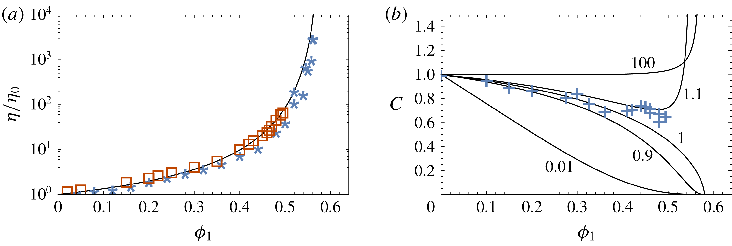
derived by Brouwers (Reference Brouwers2010) and Faroughi & Huber (Reference Faroughi and Huber2015), and is plotted in figure 5(a) along with experimental data from Segrè et al. (Reference Segrè, Meeker, Pusey and Poon1995) and Russel, Wagner & Mewis (Reference Russel, Wagner and Mewis2013). The fit is good, supporting (4.32) for the scaling factor
 $c_{d}.$
(a) Relative low-shear viscosity
 $\unicode[STIX]{x1D702}/\unicode[STIX]{x1D702}_{0}$
of a hard-sphere suspension. The curve is from (6.2); the data are from Segrè et al. (Reference Segrè, Meeker, Pusey and Poon1995) (squares) and Russel et al. (Reference Russel, Wagner and Mewis2013) (stars). (b) Parameter
 $C$
quantifying the breakdown of the Stokes–Einstein equation (6.1). When
 $C=1$
the Stokes–Einstein equation holds, while larger/smaller values of
 $C$
imply reduced/enhanced diffusion of the tracer particles. The solid curves are from (6.4); the numbers next to the curves are the values of
 $\unicode[STIX]{x1D706}_{12}$
. The data are from Segrè et al. (Reference Segrè, Meeker, Pusey and Poon1995) for the self-diffusion case
 $\unicode[STIX]{x1D706}_{12}=1$
.

In studies of the breakdown of the Stokes–Einstein relation the tracer diffusivity is often written in the form
 $$\begin{eqnarray}D_{t}=\frac{k_{B}T}{C6\unicode[STIX]{x03C0}R_{2}\unicode[STIX]{x1D702}},\end{eqnarray}$$
where
 $C=D_{SE}/D_{t}$
is a correction factor (Edward Reference Edward1970; Segrè et al.
Reference Segrè, Meeker, Pusey and Poon1995; Mackowiak, Noble & Kaufman Reference Mackowiak, Noble and Kaufman2011). Comparing with (4.16) gives
 $$\begin{eqnarray}C=\frac{\unicode[STIX]{x1D702}_{0}}{\unicode[STIX]{x1D702}\unicode[STIX]{x1D70F}}.\end{eqnarray}$$
Equation (6.4), with (6.2) for
 $\unicode[STIX]{x1D702}$
and (4.28) for
 $\unicode[STIX]{x1D70F}$
, is plotted in figure 5(b) versus
 $\unicode[STIX]{x1D719}_{1}$
for several values of the particle size ratio
 $\unicode[STIX]{x1D706}_{12}$
, along with data from Segrè et al. (Reference Segrè, Meeker, Pusey and Poon1995) for the self-diffusion case
 $\unicode[STIX]{x1D706}_{12}=1$
. The agreement is good for
 $\unicode[STIX]{x1D719}_{1}<0.4$
, providing additional support for (4.32). In the self-diffusion case
 $C$
is less than 1, implying that self-diffusion is enhanced compared to Stokes–Einstein diffusion. There is a clear breakdown of the Stokes–Einstein equation (
 $C\rightarrow 0$
) as the glass transition is approached (Kumar et al.
Reference Kumar, Szamel and Douglas2006; Mackowiak et al.
Reference Mackowiak, Noble and Kaufman2011). Near the glass transition, however, the value of
 $C$
is very sensitive to the value of
 $\unicode[STIX]{x1D706}_{12}.$
For very small tracers (
 $\unicode[STIX]{x1D706}_{12}\leqslant 0.01$
),
 $\unicode[STIX]{x1D70F}\approx 1$
and
 $C=\unicode[STIX]{x1D702}_{0}/\unicode[STIX]{x1D702}$
so that
 $D_{t}$
is equal to the Stokes–Einstein diffusivity of a tracer in the pure solvent,
 $D_{t}=k_{B}T/6\unicode[STIX]{x03C0}R_{2}\unicode[STIX]{x1D702}_{0}$
. For large tracers (
 $\unicode[STIX]{x1D706}_{12}\geqslant 100$
),
 $C=1$
over nearly the whole range in
 $\unicode[STIX]{x1D719}_{1},$
failing only as
 $\unicode[STIX]{x1D719}_{1}\rightarrow \unicode[STIX]{x1D719}_{g}$
; equation (6.4) suggests that diffusion is reduced (
 $C>1$
) for large tracers near the glass transition (Mackowiak et al.
Reference Mackowiak, Noble and Kaufman2011).
In general the tracer diffusivity can be written in the form of an effective Stokes–Einstein equation
 $$\begin{eqnarray}D_{t}=\frac{k_{B}T}{6\unicode[STIX]{x03C0}R_{2}\unicode[STIX]{x1D702}_{eff}},\end{eqnarray}$$
where
 $\unicode[STIX]{x1D702}_{eff}=C\unicode[STIX]{x1D702}=\unicode[STIX]{x1D702}_{0}/\unicode[STIX]{x1D70F}$
is an effective viscosity that depends on the tracer radius and the pore size of the host matrix (Fan et al.
Reference Fan, Dhont and Tuinier2007; Holyst et al.
Reference Holyst, Bielejewska, Szymaski, Wilk, Patkowski, Gapiski, ywociski, Kalwarczyk, Kalwarczyk and Tabaka2009; Kalwarczyk et al.
Reference Kalwarczyk, Sozanski, Jakiela, Wisniewska, Kalwarczyk, Kryszczuk, Hou and Holyst2014). Physically,
 $\unicode[STIX]{x1D70F}^{-1}=\unicode[STIX]{x1D702}_{eff}/\unicode[STIX]{x1D702}_{0}$
represents a dimensionless viscous drag force experienced by the tracer particles within the host matrix. For
 $\unicode[STIX]{x1D706}_{12}\rightarrow 0$
(vanishingly small tracer particles or infinitely large pores) the effective viscosity is equal to the pure fluid viscosity
 $\unicode[STIX]{x1D702}_{0}$
and
 $\unicode[STIX]{x1D70F}=1$
. As
 $R_{2}$
increases in a given host matrix the effective viscosity
 $\unicode[STIX]{x1D702}_{eff}$
experienced by the tracer particles also increases until, in the limit
 $R_{2}\rightarrow \infty$
,
 $\unicode[STIX]{x1D702}_{eff}$
is equal to the macroscopic viscosity
 $\unicode[STIX]{x1D702}$
of the host suspension (Kalwarczyk et al.
Reference Kalwarczyk, Sozanski, Jakiela, Wisniewska, Kalwarczyk, Kryszczuk, Hou and Holyst2014).
6.2 Physical interpretation of
 $\unicode[STIX]{x1D70E}$

A physical interpretation of the colloidal reflection coefficient
 $\unicode[STIX]{x1D70E}$
can be obtained from (3.11b
), which with (4.1), (4.7b
) and (4.9b
) can be written as
 $$\begin{eqnarray}\unicode[STIX]{x1D70E}=\frac{D_{12}}{n_{1}\unicode[STIX]{x03C0}_{2}k/\unicode[STIX]{x1D702}_{0}}=\frac{\unicode[STIX]{x1D6FC}}{K}\hat{D}_{12},\end{eqnarray}$$
so that
 $\unicode[STIX]{x1D70E}=\hat{D}_{12}$
in the limit
 $\unicode[STIX]{x1D719}_{2}\ll \unicode[STIX]{x1D719}_{1}\ll 1$
. The cross-diffusion coefficient
 $D_{12}$
quantifies diffusiophoresis – the flux of host particles induced by a gradient in tracer concentration (Anderson Reference Anderson1989; Annunziata, Buzatu & Albright Reference Annunziata, Buzatu and Albright2012). Therefore,
 $\unicode[STIX]{x1D70E}$
is a measure of the diffusiophoretic force exerted on the host matrix by the tracer particles in the pore space. Furthermore, combining (3.7a
) and (3.9b
) shows that
 $$\begin{eqnarray}\unicode[STIX]{x1D70E}=-\left(\frac{\unicode[STIX]{x1D735}\unicode[STIX]{x1D6F1}}{\unicode[STIX]{x1D735}\unicode[STIX]{x03C0}}\right)_{\boldsymbol{q}=0}.\end{eqnarray}$$
Given a tracer osmotic pressure gradient
 $\unicode[STIX]{x1D735}\unicode[STIX]{x03C0}$
in compartment B of figure 6, when
 $\unicode[STIX]{x1D70E}=0$
the tracer particles exert no force on the host matrix and
 $\unicode[STIX]{x1D735}\unicode[STIX]{x1D6F1}=0$
. Conversely, when
 $\unicode[STIX]{x1D70E}=1$
the entire tracer thermodynamic force
 $\unicode[STIX]{x1D735}\unicode[STIX]{x03C0}$
is transferred via diffusiophoresis to the host matrix, generating an equal and opposite force
 $\unicode[STIX]{x1D735}\unicode[STIX]{x1D6F1}.$
6.3 Experimental measurement of
$\unicode[STIX]{x1D70E}$

The reflection coefficient
 $\unicode[STIX]{x1D70E}(\unicode[STIX]{x1D719}_{1})$
can in principle be measured using the set-up illustrated in figure 6, which is similar to that studied numerically by Ariza & Puertas (Reference Ariza and Puertas2009) and used by Smit, Eijsermans & Staverman (Reference Smit, Eijsermans and Staverman1975) for porous media. Two reservoirs, A and C, having different pressures and tracer concentrations, are placed in contact with the suspension in B across semi-permeable partitions. The tracer concentration difference
 $\unicode[STIX]{x0394}n_{r}$
between the reservoirs leads to a diffusive flux
 $J$
. The pressure difference
 $\unicode[STIX]{x0394}p$
between the reservoirs is adjusted to ensure no volume flow (
 $q=0$
). For sufficiently small
 $\unicode[STIX]{x0394}n_{r}$
, at steady state,
 $\unicode[STIX]{x1D70E}$
is then determined from (3.9) as
 $\unicode[STIX]{x1D70E}=\unicode[STIX]{x0394}p/\unicode[STIX]{x0394}\unicode[STIX]{x03C0}=\unicode[STIX]{x0394}p/\unicode[STIX]{x0394}n_{r}k_{B}T.$
Repeating the experiment for different initial values of
 $\unicode[STIX]{x1D719}_{1}$
yields the function
 $\unicode[STIX]{x1D70E}(\unicode[STIX]{x1D719}_{1})$
. An alternative method to obtain
 $\unicode[STIX]{x1D70E}$
is to measure
 $D_{12}$
via diffusiophoresis experiments (Anderson Reference Anderson1989; Annunziata et al.
Reference Annunziata, Buzatu and Albright2012) and use (6.6). It may also be possible to obtain
 $\unicode[STIX]{x1D70E}$
from tracer sedimentation experiments, as discussed in the following section.
Illustration of a system for measuring the reflection coefficient
 $\unicode[STIX]{x1D70E}$
of a colloidal suspension. The central compartment B contains a bidisperse suspension at pressure
 $P$
and average host matrix volume fraction
 $\unicode[STIX]{x1D719}_{1}=n_{1}v_{1}$
. The partition on either side of the central compartment is permeable to the fluid and tracer particles, but impermeable to the host particles. A tracer particle concentration difference
 $\unicode[STIX]{x0394}n_{r}$
is maintained between compartments A and C, causing a steady-state tracer diffusive flux
 $J.$
A pressure difference
 $\unicode[STIX]{x0394}p$
between compartments A and C is adjusted to ensure that the volume flux
 $q$
is zero. Measurements of
 $\unicode[STIX]{x0394}n_{r}$
and
 $\unicode[STIX]{x0394}p$
then yield
 $\unicode[STIX]{x1D70E}$
via equation (3.9).

6.4 Sedimentation
As shown by Batchelor (Reference Batchelor1986), the particle fluxes in the homogeneous region of a sedimentation column are
 $$\begin{eqnarray}\displaystyle & \displaystyle n_{1}\boldsymbol{u}_{1}=\unicode[STIX]{x1D613}_{11}\boldsymbol{F}_{1}+\unicode[STIX]{x1D613}_{12}\boldsymbol{F}_{2}, & \displaystyle\end{eqnarray}$$
 $$\begin{eqnarray}\displaystyle & \displaystyle n_{2}\boldsymbol{u}_{2}=\unicode[STIX]{x1D613}_{21}\boldsymbol{F}_{1}+\unicode[STIX]{x1D613}_{22}\boldsymbol{F}_{2}, & \displaystyle\end{eqnarray}$$
 $\boldsymbol{F}_{i}=v_{i}(\unicode[STIX]{x1D70C}_{p}-\unicode[STIX]{x1D70C}_{f})\boldsymbol{g}$
is the buoyancy force acting on particle
 $i,$
with
 $\unicode[STIX]{x1D70C}_{p}$
the particle density and
 $\unicode[STIX]{x1D70C}_{f}$
the fluid density. With (2.2), (3.10), (4.1), (4.8), (4.16) and (4.34) equations (6.8) can be written as
 $$\begin{eqnarray}\displaystyle & \displaystyle \boldsymbol{u}_{1}=K\boldsymbol{u}_{1}^{0}(1+\ell n_{2}\boldsymbol{F}_{2}/n_{1}\boldsymbol{F}_{1}), & \displaystyle\end{eqnarray}$$
 $$\begin{eqnarray}\displaystyle & \displaystyle \boldsymbol{u}_{2}=\unicode[STIX]{x1D70F}\boldsymbol{u}_{2}^{0}+\ell \boldsymbol{u}_{1}, & \displaystyle\end{eqnarray}$$
 $\boldsymbol{u}_{i}^{0}=\boldsymbol{F}_{i}/6\unicode[STIX]{x03C0}R_{i}\unicode[STIX]{x1D702}_{0}$
is the Stokes velocity of particle i in the fluid. Given
 $\unicode[STIX]{x1D70F}(\unicode[STIX]{x1D719}_{1})$
, measurements of
 $\boldsymbol{u}_{i}$
can therefore be used in (6.9b
) to determine the cross-diffusion factor
 $\ell$
; given
 $\unicode[STIX]{x1D6FC}(\unicode[STIX]{x1D719}_{1}),$
the reflection coefficient can then be obtained from (4.34) as
 $\unicode[STIX]{x1D70E}=1-\unicode[STIX]{x1D6FC}(1-\ell )$
.
It is interesting to consider very concentrated suspensions with
 $\unicode[STIX]{x1D719}_{1}\geqslant \unicode[STIX]{x1D719}_{1}^{c}$
, in which case
 $\unicode[STIX]{x1D70F}=0$
,
 $\unicode[STIX]{x1D70E}=1$
and the tracer particles are trapped in the pores (§ 4.5). Equation (4.34) gives
 $\ell =1$
and (6.9b
) becomes
 $\boldsymbol{u}_{2}=\boldsymbol{u}_{1}$
, so that the tracer particles are constrained to sediment at the same speed as the host particles (Kaye & Davies Reference Kaye and Davies1972; Lockett & Al-Habbooby Reference Lockett and Al-Habbooby1974; Snabre et al.
Reference Snabre, Pouligny, Metayer and Nadal2009). Figure 3(b) shows data for the critical trapping volume fraction at which
 $\boldsymbol{u}_{2}=\boldsymbol{u}_{1}$
in the sedimentation experiments of Lockett & Al-Habbooby (Reference Lockett and Al-Habbooby1974) (squares). The data lie close to the lower curve in figure 3(b), suggesting that the expressions for
 $\unicode[STIX]{x1D70E}$
and
 $\unicode[STIX]{x1D70F}$
developed for porous media, equations (4.25) and (4.26), may be appropriate in this case rather than the suspension equations (4.28) and (4.29). This can be explained by the Péclet number,
 $Pe=u_{1}R_{1}/D_{1}^{0},$
which was approximately
 $10^{8}$
in their system (Lockett & Al-Habbooby Reference Lockett and Al-Habbooby1974). The time scale for sedimentation of the particles was therefore much faster than the time scale for diffusive heterogeneities to appear, and the host matrix may have behaved effectively like a porous medium.
7 Conclusion
Equations for the diffusion and cross-diffusion coefficients
 $D_{ij}$
of tracer particles in hard-sphere suspensions have been obtained as functions of the host-particle volume fraction
 $\unicode[STIX]{x1D719}_{1}$
and particle size ratio
 $\unicode[STIX]{x1D706}_{12}=R_{2}/R_{1}$
. By transforming the chemical potentials and phenomenological coefficients into more experimentally convenient quantities such as the permeability
 $k$
and osmotic pressure
 $\unicode[STIX]{x1D6F1}$
, expressions have been obtained for the diffusion coefficients at volume fractions up to the close-packing limit. These expressions contain the reflection coefficient
 $\unicode[STIX]{x1D70E};$
a brief discussion of the physical interpretation and experimental measurement of
 $\unicode[STIX]{x1D70E}$
in suspensions has been included. The tracer Fickian diffusivity
 $D_{t}$
can be written in the form of an effective Stokes–Einstein equation,
 $D_{t}=k_{B}T/6\unicode[STIX]{x03C0}R_{2}\unicode[STIX]{x1D702}_{eff}$
, where
 $\unicode[STIX]{x1D702}_{eff}$
is the effective viscosity experienced by the tracer particle in the host matrix. Tracer Fickian diffusion and segregation during sedimentation cease at a critical trapping volume fraction
 $\unicode[STIX]{x1D719}_{1}^{c}$
, which depends on the effective pore size in the suspension and represents an effective glass transition of the tracer particles. Cross-diffusion of the tracer particles may become increasingly important relative to Fickian diffusion at volume fractions near to and above
 $\unicode[STIX]{x1D719}_{1}^{c}$
.
Acknowledgements
I thank the University of Toronto Mississauga for providing computing facilities and gratefully acknowledge M. G. Worster, J. S. Wettlaufer, J. R. Ockendon, S. Liu, W.-C. Lin, H.-E. Lin, D. W. Lawther, C. S. Lai, J. A. W. Elliott and D. Dahn for inspiring this work, as well as the anonymous referees for valuable suggestions.