1 Introduction
We consider periodic waves at the surface of an incompressible inviscid fluid in two dimensions, propagating with permanent form a long distance at a practically constant velocity. Studies of gravity waves in an irrotational flow date back to Stokes (Reference Stokes1847, Reference Stokes1880) and others, and an immense amount of progress has been made over the past one and a half centuries. Particularly, Stokes’ conjecture about the so-called wave of greatest height or extreme wave was rigorously proved. Yet the steady water wave problem still poses many great difficulties. For instance, there are very few exact solutions or approximate solutions for nearly extreme waves. Such solutions are an invaluable tool both from a numerical and analytical point of view.
Gerstner (Reference Gerstner1802) (see also Constantin Reference Constantin2001) produced an interesting example of gravity waves with non-zero vorticity. The fluid particles for the solution move in perfect circles whose radius decreases with depth, which are explicitly expressible in Lagrangian coordinates. Moreover, any streamline for the solution can itself be taken as a free surface and those below it as streamlines, up until the ‘limiting’ configuration for which the vorticity becomes unbounded and the crest degenerates into a cusp.
On the other hand, Crapper (Reference Crapper1957) discovered a striking and surprising exact solution for capillary waves in an irrotational flow when gravitational acceleration is negligible. The fluid flow for the solution is given in a concise form in terms of a conformal mapping in Eulerian coordinates. Like Gerstner waves, any streamline of Crapper’s solution can be taken as a free surface, up to the limiting wave whose free surface encloses a bubble of air at the trough. Although Crapper waves solve a highly idealized problem without gravity or fixed boundaries, they have nevertheless been instrumental when studying the combined effects of gravity and surface tension (see Chen & Saffman Reference Chen and Saffman1979, Reference Chen and Saffman1980; Schwartz & Vanden-Broeck Reference Schwartz and Vanden-Broeck1979; Longuet-Higgins Reference Longuet-Higgins1992, among others).
To the best of the authors’ knowledge, no other solutions are known explicitly for steady water waves in infinite depth. However, we note that Kinnersley (Reference Kinnersley1976) generalized Crapper’s solution to finite depth (involving elliptic functions).
Recently, Dyachenko & Hur (Reference Dyachenko and Hur2019b,Reference Dyachenko and Hurc) (see also Dyachenko & Hur Reference Dyachenko and Hur2019a) found numerically a family of gravity waves with constant vorticity, in the absence of the effects of surface tension, whose free surface approaches the limiting Crapper wave in an irrotational flow as gravitational acceleration vanishes. Hur & Vanden-Broeck (Reference Hur and Vanden-Broeck2020) took matters further and provided numerical and asymptotic evidence of a new exact solution. The free surface for such solution would be the same as the Crapper wave, but the physical setting and fluid flow would be altogether different. Like Crapper waves, there is no gravitational acceleration, but now there is no surface tension either. Instead, the rounded shape of the free surface is sustained by constant vorticity. Such a connection between rotational and capillary effects is remarkable and wholly unexpected, and remains to be fully explained.
Here we analytically confirm that there is indeed an exact solution of this kind. For a fluid region bounded by a Crapper wave, we find a stream function explicitly in conformal variables (see (4.5)) which has constant vorticity, the desired asymptotics at great depths, and which satisfies the kinematic boundary condition on the free surface. Substituting into the dynamic boundary condition, we are able to solve the problem and determine the value of constant vorticity (see (4.8)). Moreover, the stream function formula allows us a detailed description of the fluid flow beneath the wave, which exhibits Kelvin’s cat’s eye streamline pattern. Such flow pattern beneath gravity waves with constant vorticity has previously been studied both analytically (Wahlén Reference Wahlén2009, and others) and numerically (Ribeiro, Milewski & Nachbin Reference Ribeiro, Milewski and Nachbin2017, and others).
While our new exact solution solves a highly idealized problem, neglecting gravity and fixed boundaries, we believe that, like Crapper waves, it will be significant when investigating more physically realistic scenarios. For instance, by perturbing the solution with gravity, as Akers, Ambrose & Wright (Reference Akers, Ambrose and Wright2014) did for capillary waves in an irrotational flow, it may be possible to prove the existence of overhanging gravity waves with constant vorticity. Such waves have long been suggested by numerical computations (see Simmen & Saffman Reference Simmen and Saffman1985; Teles da Silva & Peregrine Reference Teles da Silva and Peregrine1988; Dyachenko & Hur Reference Dyachenko and Hur2019c, among others), but so far a rigorous proof has been elusive (Constantin, Strauss & Vărvărucă Reference Constantin, Strauss and Vărvărucă2016). Another future direction is to attempt to, as Kinnersley (Reference Kinnersley1976) did for capillary waves, find an analogous exact solution in finite depth. From Teles da Silva & Peregrine (Reference Teles da Silva and Peregrine1988), however, we expect that our solution in infinite depth will well approximate those in finite depth as soon as the depth is moderately large.
2 Formulation and conformal mapping
We consider an incompressible inviscid fluid of constant density  $\unicode[STIX]{x1D70C}$ which occupies a region
 $D$ in
 $\mathbb{R}^{2}$, bounded by a free surface
 $S$, and a wave propagating along
 $S$. Suppose for definiteness that in Cartesian coordinates, the
 $x$ axis points in the direction of wave propagation and the
 $y$ axis vertically upwards. Working in a moving reference frame, we may assume that the wave is stationary and give
 $S$ a parametrization
 $x=x(\unicode[STIX]{x1D6FC})$ and
 $y=y(\unicode[STIX]{x1D6FC})$, where
 $\unicode[STIX]{x1D6FC}\in \mathbb{R}$. We assume that there are no outside forces acting on the fluid (for instance, gravity) so that the velocity of the fluid
 $(u,v)$ and the pressure
 $P$ satisfy the Euler equations for an incompressible fluid:
 $$\begin{eqnarray}\left\{\begin{array}{@{}l@{}}\unicode[STIX]{x1D70C}(uu_{x}+vu_{y})=-P_{x}\\ \unicode[STIX]{x1D70C}(uv_{x}+vv_{y})=-P_{y}\end{array}\right.\quad \text{and}\quad u_{x}+v_{y}=0\text{ in }D.\end{eqnarray}$$
We additionally assume that the scalar vorticity
 $$\begin{eqnarray}\unicode[STIX]{x1D714}=v_{x}-u_{y}\end{eqnarray}$$
is a constant. Requiring that each fluid particle on  $S$ remains on
 $S$, we have a kinematic boundary condition, which can, for instance, be expressed as
 $$\begin{eqnarray}uy_{\unicode[STIX]{x1D6FC}}-vx_{\unicode[STIX]{x1D6FC}}=0\quad \text{ on }S.\end{eqnarray}$$
At great depths, we instead require
 $$\begin{eqnarray}(u+\unicode[STIX]{x1D714}y+c,v)\rightarrow (0,0)\quad \text{ as }y\rightarrow -\infty\end{eqnarray}$$
for some constant  $c$. When
 $\unicode[STIX]{x1D714}=0$,
 $c$ is the speed of the wave in a frame where the fluid is at rest at the infinite bottom. Finally, we require the dynamic boundary condition
 $$\begin{eqnarray}P=\text{constant}-T\unicode[STIX]{x1D705}\quad \text{ on }S,\end{eqnarray}$$
where  $T\geqslant 0$ is the coefficient of surface tension and
 $$\begin{eqnarray}\unicode[STIX]{x1D705}=\frac{x_{\unicode[STIX]{x1D6FC}}y_{\unicode[STIX]{x1D6FC}\unicode[STIX]{x1D6FC}}-y_{\unicode[STIX]{x1D6FC}}x_{\unicode[STIX]{x1D6FC}\unicode[STIX]{x1D6FC}}}{(x_{\unicode[STIX]{x1D6FC}}^{2}+y_{\unicode[STIX]{x1D6FC}}^{2})^{3/2}}\end{eqnarray}$$
is the curvature of  $S$. Throughout we will be interested in motions which are furthermore periodic in
 $x$, and we let
 $k$ be the associated wavenumber.
The second equation in (2.1a) allows us to introduce a stream function, defined by
 $$\begin{eqnarray}\unicode[STIX]{x1D713}_{x}=-v\quad \text{and}\quad \unicode[STIX]{x1D713}_{y}=u.\end{eqnarray}$$
Moreover, (2.1c) allows us to normalize  $\unicode[STIX]{x1D713}$ so that it vanishes on
 $S$. The first equations in (2.1a) then imply that
 $$\begin{eqnarray}\frac{1}{2}|\unicode[STIX]{x1D735}\unicode[STIX]{x1D713}|^{2}+\unicode[STIX]{x1D714}\unicode[STIX]{x1D713}+\frac{P}{\unicode[STIX]{x1D70C}}=\text{constant}\end{eqnarray}$$
throughout  $D$. Switching to dimensionless units with length scale
 $1/k$ and velocity scale
 $c$, (2.1) becomes
 $$\begin{eqnarray}\displaystyle \displaystyle & & \displaystyle \unicode[STIX]{x1D6FB}^{2}\unicode[STIX]{x1D713}=-\unicode[STIX]{x1D6FA}\hspace{45.52458pt}\,\text{in }D,\end{eqnarray}$$
 $$\begin{eqnarray}\displaystyle \displaystyle & & \displaystyle \unicode[STIX]{x1D713}=0\hspace{71.13188pt}\,\text{ on }S,\end{eqnarray}$$
 $$\begin{eqnarray}\displaystyle \displaystyle & & \displaystyle \unicode[STIX]{x1D713}_{y}+\unicode[STIX]{x1D6FA}y+1\rightarrow 0\qquad \text{ as }y\rightarrow -\infty ,\end{eqnarray}$$
 $$\begin{eqnarray}\displaystyle \displaystyle & & \displaystyle {\textstyle \frac{1}{2}}|\unicode[STIX]{x1D735}\unicode[STIX]{x1D713}|^{2}-\unicode[STIX]{x1D70F}\unicode[STIX]{x1D705}=B\qquad \text{ on }S.\end{eqnarray}$$
 $B$ is a dimensionless Bernoulli constant, and
 $$\begin{eqnarray}\unicode[STIX]{x1D6FA}=\frac{\unicode[STIX]{x1D714}}{ck}\quad \text{and}\quad \unicode[STIX]{x1D70F}=\frac{Tk}{\unicode[STIX]{x1D70C}c^{2}}\end{eqnarray}$$
are the dimensionless vorticity and surface tension coefficient. Furthermore,  $\unicode[STIX]{x1D713}$,
 $D$ and
 $S$ are
 $2\unicode[STIX]{x03C0}$ periodic in
 $x$.
Identifying  $\mathbb{R}^{2}$ with the complex plane, in what follows let
 $z=x+\text{i}y$ and suppose that
 $$\begin{eqnarray}z=z(\unicode[STIX]{x1D6FC}+\text{i}\unicode[STIX]{x1D6FD})\end{eqnarray}$$
conformally maps the lower half-plane  $\{\unicode[STIX]{x1D6FC}+\text{i}\unicode[STIX]{x1D6FD}:\unicode[STIX]{x1D6FD}<0\}$ to
 $D$ and that
 $S$ is the restriction of the conformal mapping to
 $\unicode[STIX]{x1D6FD}=0$. We normalize the mapping by requiring that
 $z(\unicode[STIX]{x1D6FC}+\text{i}\unicode[STIX]{x1D6FD})\sim \unicode[STIX]{x1D6FC}+\text{i}\unicode[STIX]{x1D6FD}$ as
 $\unicode[STIX]{x1D6FD}\rightarrow -\infty$ and that
 $x(\unicode[STIX]{x1D6FC})-\unicode[STIX]{x1D6FC}$ and
 $y(\unicode[STIX]{x1D6FC})$ are
 $2\unicode[STIX]{x03C0}$ periodic. For later use, we calculate
 $$\begin{eqnarray}|\unicode[STIX]{x1D6FB}_{(x,y)}\unicode[STIX]{x1D713}|^{2}=\frac{\unicode[STIX]{x1D713}_{\unicode[STIX]{x1D6FD}}^{2}}{|z_{\unicode[STIX]{x1D6FC}}|^{2}}\quad \text{ on }S.\end{eqnarray}$$
This follows from (2.2b) and that  $z(\unicode[STIX]{x1D6FC}+\text{i}\unicode[STIX]{x1D6FD})$ is complex analytic.
3 Crapper’s capillary waves in an irrotational flow
When  $\unicode[STIX]{x1D6FA}=0$ (irrotational flow), note that
 $$\begin{eqnarray}\unicode[STIX]{x1D713}=-\unicode[STIX]{x1D6FD}\end{eqnarray}$$
solves (2.2a)–(2.2c). Plugging into (2.2d) and using (2.3), we arrive at
 $$\begin{eqnarray}\frac{1}{2}\frac{1}{|z_{\unicode[STIX]{x1D6FC}}|^{2}}-\unicode[STIX]{x1D70F}\frac{x_{\unicode[STIX]{x1D6FC}}y_{\unicode[STIX]{x1D6FC}\unicode[STIX]{x1D6FC}}-y_{\unicode[STIX]{x1D6FC}}x_{\unicode[STIX]{x1D6FC}\unicode[STIX]{x1D6FC}}}{|z_{\unicode[STIX]{x1D6FC}}|^{3}}=B\quad \text{ on }\unicode[STIX]{x1D6FD}=0.\end{eqnarray}$$
One can then verify that, for any  $A\geqslant 0$, the parametric curve due to Crapper (Reference Crapper1957)
 $$\begin{eqnarray}z(\unicode[STIX]{x1D6FC})=\unicode[STIX]{x1D6FC}-4\text{i}A\frac{\text{e}^{-\text{i}\unicode[STIX]{x1D6FC}}}{1+A\text{e}^{-\text{i}\unicode[STIX]{x1D6FC}}}\end{eqnarray}$$
extends conformally to the lower half plane and solves (3.2), where
 $$\begin{eqnarray}\unicode[STIX]{x1D70F}=\frac{1+A^{2}}{1-A^{2}}\quad \text{and}\quad B=\frac{1}{2}.\end{eqnarray}$$
Therefore,  $z=z(\unicode[STIX]{x1D6FC}+\text{i}\unicode[STIX]{x1D6FD})$, where
 $z$ is in (3.3), and (3.1) together make an exact solution of (2.2) when
 $\unicode[STIX]{x1D6FA}=0$ and
 $\unicode[STIX]{x1D70F}\neq 0$. For
 $A>A_{max}\approx 0.4546700164520109$, however, the free surface intersects itself and the fluid flow becomes multi-valued, whence the solution is physically unrealistic.
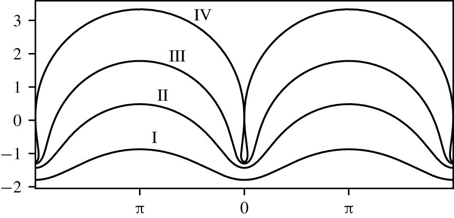
Streamlines for the limiting Crapper wave. Curve IV is the free surface. Alternatively, after an appropriate vertical shift, curves I, II and III may be thought of as the free surface for the Crapper wave for different values of  $A$ and
 $\unicode[STIX]{x1D70F}$.

We observe that the streamlines for the solution are simply the curves  $z=z(\unicode[STIX]{x1D6FC}+\text{i}\unicode[STIX]{x1D6FD})$ for fixed
 $\unicode[STIX]{x1D6FD}({<}0)$ and that any of these streamlines can itself be thought of as a free surface, albeit for a different choice of
 $\unicode[STIX]{x1D70F}$. This is because (3.3) enjoys
 $z(\unicode[STIX]{x1D6FC}+\text{i}\unicode[STIX]{x1D6FD};A)=z(\unicode[STIX]{x1D6FC};e^{\unicode[STIX]{x1D6FD}}A)+\text{i}\unicode[STIX]{x1D6FD}$. Figure 1 provides some examples.
4 Waves in constant vorticity flows
We continue to suppose the conformal mapping  $z=z(\unicode[STIX]{x1D6FC}+\text{i}\unicode[STIX]{x1D6FD})$, where
 $z$ is in (3.3), but now set
 $\unicode[STIX]{x1D70F}=0$ and
 $\unicode[STIX]{x1D6FA}\neq 0$. Note that
 $$\begin{eqnarray}\unicode[STIX]{x1D713}=-{\textstyle \frac{1}{2}}\unicode[STIX]{x1D6FA}y^{2}-y-f\end{eqnarray}$$
solves (2.2a)–(2.2c), provided that  $f$ (uniquely) solves
 $$\begin{eqnarray}\left\{\begin{array}{@{}ll@{}}\unicode[STIX]{x1D6FB}^{2}f=0\quad & \text{ in }D,\\ f=-\frac{1}{2}\unicode[STIX]{x1D6FA}y^{2}-y\quad & \text{ on }S,\\ \unicode[STIX]{x1D735}f\rightarrow 0\quad & \text{ as }y\rightarrow -\infty .\end{array}\right.\end{eqnarray}$$
To calculate  $f$, it is convenient to view it as a function of the variable
 $$\begin{eqnarray}\unicode[STIX]{x1D701}=\text{e}^{\text{i}(\unicode[STIX]{x1D6FC}+\text{i}\unicode[STIX]{x1D6FD})}\end{eqnarray}$$
taking values in the unit disk. The surface  $S$ corresponds to the unit circle
 $|\unicode[STIX]{x1D701}|=1$, where (3.3) gives
 $$\begin{eqnarray}y=\text{Im}\left(\unicode[STIX]{x1D6FC}-\frac{4\text{i}A}{\unicode[STIX]{x1D701}+A}\right)=-\frac{2(\unicode[STIX]{x1D701}^{2}+2A\unicode[STIX]{x1D701}+1)}{(\unicode[STIX]{x1D701}+A)(\unicode[STIX]{x1D701}+1/A)}\end{eqnarray}$$
and hence
 $$\begin{eqnarray}f(\unicode[STIX]{x1D701})=-\frac{1}{2}\unicode[STIX]{x1D6FA}y^{2}-y=-\frac{2(\unicode[STIX]{x1D701}+2A\unicode[STIX]{x1D701}+1)^{2}}{(\unicode[STIX]{x1D701}+A)^{2}(\unicode[STIX]{x1D701}+1/A)^{2}}\unicode[STIX]{x1D6FA}+\frac{2(\unicode[STIX]{x1D701}+2A\unicode[STIX]{x1D701}+1)}{(\unicode[STIX]{x1D701}+A)(\unicode[STIX]{x1D701}+1/A)}.\end{eqnarray}$$
The values of  $f$ in the unit disk can then be calculated using the Poisson integral formula
 $$\begin{eqnarray}f(\unicode[STIX]{x1D701})=\text{Re}\left(\frac{1}{2\unicode[STIX]{x03C0}\text{i}}\oint _{|\unicode[STIX]{x1D701}^{\prime }|=1}f(\unicode[STIX]{x1D701}^{\prime })\frac{\unicode[STIX]{x1D701}^{\prime }+\unicode[STIX]{x1D701}}{\unicode[STIX]{x1D701}^{\prime }-\unicode[STIX]{x1D701}}\frac{\text{d}\unicode[STIX]{x1D701}^{\prime }}{\unicode[STIX]{x1D701}^{\prime }}\right).\end{eqnarray}$$
Note that for  $0<A<A_{max}<1$, the only poles of the integrand in (4.4) with
 $|\unicode[STIX]{x1D701}^{\prime }|<1$ are at
 $\unicode[STIX]{x1D701}^{\prime }=0$ and
 $\unicode[STIX]{x1D701}^{\prime }=-A$. Using the calculus of residues to evaluate the integral, we obtain
 $$\begin{eqnarray}f(\unicode[STIX]{x1D701})=\text{Re}\left(\frac{4\unicode[STIX]{x1D6FA}A^{2}}{A^{2}-1}\frac{\unicode[STIX]{x1D701}^{2}-2A^{2}+1}{(\unicode[STIX]{x1D701}+A)^{2}}+\frac{4A}{\unicode[STIX]{x1D701}+A}\right).\end{eqnarray}$$
Substitution into (4.1) then yields
 $$\begin{eqnarray}\unicode[STIX]{x1D713}=-\unicode[STIX]{x1D6FD}-\frac{1}{2}\unicode[STIX]{x1D6FA}y^{2}-\frac{4\unicode[STIX]{x1D6FA}A^{2}}{A^{2}-1}\text{Re}\left(\frac{\unicode[STIX]{x1D701}^{2}-2A^{2}+1}{(\unicode[STIX]{x1D701}+A)^{2}}\right),\end{eqnarray}$$
where we have simplified using  $y=\unicode[STIX]{x1D6FD}-\text{Re}(4A/(\unicode[STIX]{x1D701}+A))$.
Differentiating (4.5) using  $\unicode[STIX]{x2202}\unicode[STIX]{x1D701}/\unicode[STIX]{x2202}\unicode[STIX]{x1D6FD}=-\unicode[STIX]{x1D701}$, we calculate
 $$\begin{eqnarray}\unicode[STIX]{x1D713}_{\unicode[STIX]{x1D6FD}}=-1-\unicode[STIX]{x1D6FA}yx_{\unicode[STIX]{x1D6FC}}+\frac{8\unicode[STIX]{x1D6FA}A^{2}}{A^{2}-1}\text{Re}\left(\frac{\unicode[STIX]{x1D701}(A\unicode[STIX]{x1D701}+2A^{2}-1)}{(\unicode[STIX]{x1D701}+A)^{3}}\right),\end{eqnarray}$$
so that (2.2d) becomes, by (2.3),
 $$\begin{eqnarray}\left(-1-\unicode[STIX]{x1D6FA}yx_{\unicode[STIX]{x1D6FC}}+\frac{8\unicode[STIX]{x1D6FA}A^{2}}{A^{2}-1}\text{Re}\left(\frac{\unicode[STIX]{x1D701}(A\unicode[STIX]{x1D701}+2A^{2}-1)}{(\unicode[STIX]{x1D701}+A)^{3}}\right)\right)^{2}=\frac{1}{2}B|z_{\unicode[STIX]{x1D6FC}}|^{2}\quad \text{ on }\unicode[STIX]{x1D6FD}=0.\end{eqnarray}$$
Inserting (3.3) leaves us with
 $$\begin{eqnarray}\bigg(-1+2\unicode[STIX]{x1D6FA}\frac{\unicode[STIX]{x1D701}^{2}+2A\frac{A^{2}+1}{A^{2}-1}\unicode[STIX]{x1D701}+1}{(\unicode[STIX]{x1D701}+A)(\unicode[STIX]{x1D701}+1/A)}\bigg)^{2}=2B\frac{(\unicode[STIX]{x1D701}-A)^{2}(\unicode[STIX]{x1D701}-1/A)^{2}}{(\unicode[STIX]{x1D701}+A)^{2}(\unicode[STIX]{x1D701}+1/A)^{2}},\end{eqnarray}$$
which must hold for all  $|\unicode[STIX]{x1D701}|=1$. Indeed, since the two sides of (4.7) are rational functions of
 $\unicode[STIX]{x1D701}$, the equation must hold for all
 $\unicode[STIX]{x1D701}\in \mathbb{C}$ where the denominators do not vanish. Plugging in
 $\unicode[STIX]{x1D701}=0$ and
 $\unicode[STIX]{x1D701}=A$, and recalling that
 $0<A<A_{max}<1/2$, we find at once that
 $$\begin{eqnarray}\unicode[STIX]{x1D6FA}=\frac{1-A^{2}}{1-3A^{2}}\quad \text{and}\quad B=\frac{1}{2}\left(\frac{1+A^{2}}{1-3A^{2}}\right)^{2}.\end{eqnarray}$$
Note that  $\unicode[STIX]{x1D6FA}>0$. Somewhat miraculously, a direct calculation shows that the choice (4.8) in fact solves (4.7) for all
 $\unicode[STIX]{x1D701}$ where the denominators do not vanish. In particular, (4.6) holds and hence
 $\unicode[STIX]{x1D713}$ solves (2.2).
To recapitulate,  $z=z(\unicode[STIX]{x1D6FC}+\text{i}\unicode[STIX]{x1D6FD})$, where
 $z$ is in (3.3), and (4.5) together make a new exact solution of (2.2) when
 $\unicode[STIX]{x1D6FA}>0$ and
 $\unicode[STIX]{x1D70F}=0$. The vorticity
 $\unicode[STIX]{x1D6FA}$ and Bernoulli constant
 $B$ are specified in terms of
 $0<A<A_{max}$ by (4.8), yielding a one-parameter family of solutions.
5 The fluid flow beneath the waves
Free surfaces and streamlines, in the  $(x,y)$ plane, for the new exact solutions in (4.5) for
 $A=A_{max}/4$,
 $A_{max}/2$,
 $3A_{max}/4$ and
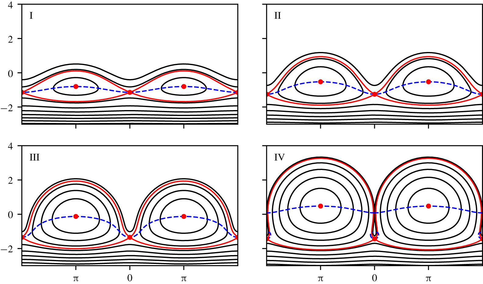
 $A_{max}$. Up to a vertical shift, the free surfaces I–IV coincide with the streamlines I–IV for the Crapper wave in figure 1. The stagnation points are shown in red, together with the heteroclinic connections between the saddle points. These heteroclinic orbits enclose a so-called critical layer of closed streamlines, which in particular contains the dashed blue curve across which the horizontal velocity changes sign.

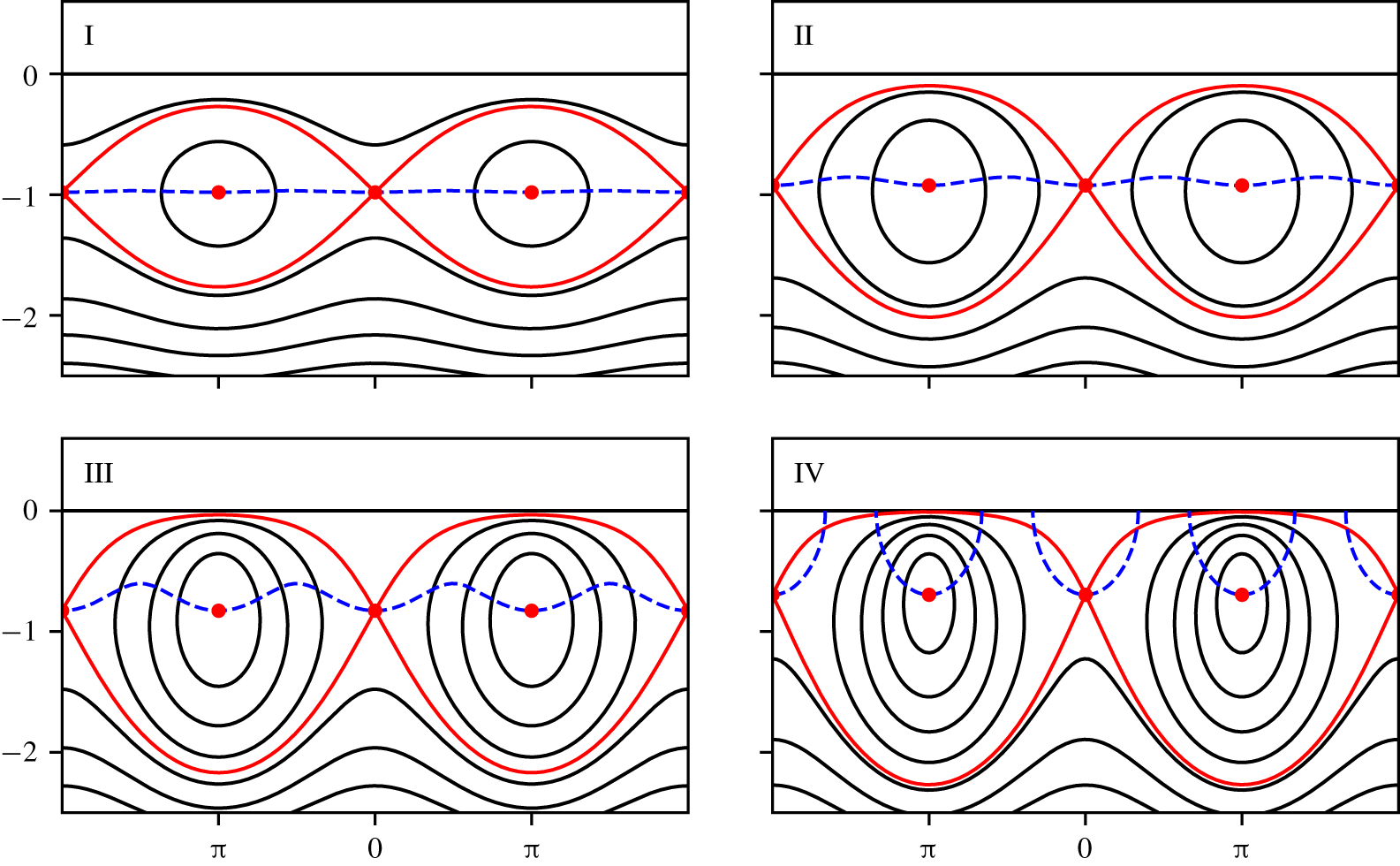
Since we have an explicit formula (4.5) for the stream function, it is straightforward to plot streamlines. Figure 2 shows the streamlines associated with the Crapper wave profiles I–IV in figure 1 in the  $(x,y)$ plane, while figure 3 shows the same streamlines in the
 $(\unicode[STIX]{x1D6FC},\unicode[STIX]{x1D6FD})$ plane.
The examples from figure 2 in the  $(\unicode[STIX]{x1D6FC},\unicode[STIX]{x1D6FD})$ plane. Here the streamline
 $\unicode[STIX]{x1D6FD}=0$ corresponds to the free surface. Note that the stagnation points in a given wave all have the same value of
 $\unicode[STIX]{x1D6FD}$.

Unlike for Crapper’s capillary waves in an irrotational flow, there are now closed streamlines as well as stagnation points, where  $\unicode[STIX]{x1D713}_{x}=\unicode[STIX]{x1D713}_{y}=0$ or, equivalently,
 $\unicode[STIX]{x1D713}_{\unicode[STIX]{x1D6FC}}=\unicode[STIX]{x1D713}_{\unicode[STIX]{x1D6FD}}=0$. Since
 $y_{\unicode[STIX]{x1D6FC}}(\unicode[STIX]{x1D6FC}+\text{i}0)$ alternates sign on each half-period, a maximum principle argument shows that the same is true of
 $\unicode[STIX]{x1D713}_{\unicode[STIX]{x1D6FC}}$ as well as the vertical velocity
 $v=-\unicode[STIX]{x1D713}_{x}$. Hence, stagnation points can only occur on the vertical lines
 $x=\unicode[STIX]{x1D6FC}=\pm \unicode[STIX]{x03C0},\pm 3\unicode[STIX]{x03C0},\ldots$ below the crests or the lines
 $x=\unicode[STIX]{x1D6FC}=\pm 2\unicode[STIX]{x03C0},\pm 4\unicode[STIX]{x03C0},\ldots$ below the troughs. In either case, they can be calculated numerically using a simple root-finding algorithm. Interestingly, the stagnation point below the crest and the stagnation point below the trough have precisely the same value of
 $\unicode[STIX]{x1D6FD}$, as can be confirmed analytically by calculating the ratio
 $$\begin{eqnarray}\frac{\unicode[STIX]{x1D713}_{\unicode[STIX]{x1D6FD}}(\unicode[STIX]{x03C0},\unicode[STIX]{x1D6FD})}{\unicode[STIX]{x1D713}_{\unicode[STIX]{x1D6FD}}(0,\unicode[STIX]{x1D6FD})}=\bigg(\frac{1+Ae^{\unicode[STIX]{x1D6FD}}}{1-Ae^{\unicode[STIX]{x1D6FD}}}\bigg)^{4}>0.\end{eqnarray}$$
The stagnation points below the troughs are saddles, and are connected by pairs of heteroclinic orbits enclosing regions of closed streamlines. The dashed blue curve in the figures shows where the horizontal velocity
 $$\begin{eqnarray}u=\unicode[STIX]{x1D713}_{y}=\frac{\unicode[STIX]{x1D713}_{\unicode[STIX]{x1D6FC}}y_{\unicode[STIX]{x1D6FC}}+\unicode[STIX]{x1D713}_{\unicode[STIX]{x1D6FD}}x_{\unicode[STIX]{x1D6FC}}}{x_{\unicode[STIX]{x1D6FC}}^{2}+y_{\unicode[STIX]{x1D6FC}}^{2}}\end{eqnarray}$$
vanishes. It is a single closed curve in cases I–III where the surface is single-valued, but not for the overhanging wave in IV.
6 Remark on a single equation for constant vorticity
In § 3, in an irrotational flow, the boundary-value problem (2.1) for the stream function and the free surface reduced to a single equation (3.2) for the conformal parametrization of the free surface alone. In § 4, in a constant vorticity flow, on the other hand, we inserted the ansatz (3.3) and solved (2.1) for the stream function. A single equation does exist for constant vorticity (see Dyachenko & Hur Reference Dyachenko and Hur2019b,Reference Dyachenko and Hurc, for instance), however, and in our notation can be written
 $$\begin{eqnarray}\frac{1}{2}\frac{\big(1+\unicode[STIX]{x1D6FA}\big(yx_{\unicode[STIX]{x1D6FC}}-{\mathcal{H}}(yy_{\unicode[STIX]{x1D6FC}})\big)\big)^{2}}{|z_{\unicode[STIX]{x1D6FC}}|^{2}}=B\quad \text{on }\unicode[STIX]{x1D6FD}=0.\end{eqnarray}$$
Here  ${\mathcal{H}}$ is the periodic Hilbert transform, defined by
 $$\begin{eqnarray}{\mathcal{H}}f(\unicode[STIX]{x1D6FC})=\frac{1}{2\unicode[STIX]{x03C0}}\operatorname{PV}\int _{-\unicode[STIX]{x03C0}}^{\unicode[STIX]{x03C0}}f(\unicode[STIX]{x1D6FC}^{\prime })\cot \left(\frac{\unicode[STIX]{x1D6FC}-\unicode[STIX]{x1D6FC}^{\prime }}{2}\right)\text{d}\unicode[STIX]{x1D6FC}^{\prime },\end{eqnarray}$$
where  $\operatorname{PV}$ means the principal value integral. Using
 $x(\unicode[STIX]{x1D6FC})=\unicode[STIX]{x1D6FC}+{\mathcal{H}}y(\unicode[STIX]{x1D6FC})$, one can in fact write (6.1) (or indeed (3.2)) in terms of
 $y$ alone.
By the argument in the previous section, the conformal mapping in (3.3) satisfies (6.1), provided that  $\unicode[STIX]{x1D6FA}$ and
 $B$ are in (4.8). This can also be verified directly. It is convenient to introduce
 $\unicode[STIX]{x1D701}=\text{e}^{\text{i}(\unicode[STIX]{x1D6FC}+\text{i}\unicode[STIX]{x1D6FD})}$ as before, so that (3.3) means
 $y(\unicode[STIX]{x1D6FC})$ is given by (4.3). We use the Plemelj formula (see King Reference King2009, chap. 3, for instance, for details) to find that for
 $|\unicode[STIX]{x1D701}|=1$,
 $$\begin{eqnarray}\displaystyle {\mathcal{H}}f(\unicode[STIX]{x1D701}) & = & \displaystyle \frac{1}{\unicode[STIX]{x03C0}}\operatorname{PV}\oint _{|\unicode[STIX]{x1D701}^{\prime }|=1}\frac{f(\unicode[STIX]{x1D701}^{\prime })}{\unicode[STIX]{x1D701}-\unicode[STIX]{x1D701}^{\prime }}\,\text{d}\unicode[STIX]{x1D701}^{\prime }\nonumber\\ \displaystyle & = & \displaystyle \frac{1}{\unicode[STIX]{x03C0}}\lim _{r\rightarrow 1}\oint _{|\unicode[STIX]{x1D701}^{\prime }|=r<1}\frac{f(\unicode[STIX]{x1D701}^{\prime })}{\unicode[STIX]{x1D701}-\unicode[STIX]{x1D701}^{\prime }}\,\text{d}\unicode[STIX]{x1D701}^{\prime }-\text{i}f(\unicode[STIX]{x1D701}).\nonumber\end{eqnarray}$$
We can then evaluate the Hilbert transform using the calculus of residues. In particular,
 $$\begin{eqnarray}y{\mathcal{H}}y_{\unicode[STIX]{x1D6FC}}-{\mathcal{H}}(yy_{\unicode[STIX]{x1D6FC}})=\frac{-8A\unicode[STIX]{x1D701}}{(A^{2}-1)(\unicode[STIX]{x1D701}+A)(\unicode[STIX]{x1D701}+1/A)}.\end{eqnarray}$$
We omit the details.
7 Summary
We have found a new exact solution for periodic travelling waves in a constant vorticity flow of infinite depth, in the absence of the effects of gravity or surface tension, confirming numerical and asymptotic evidence (Dyachenko & Hur Reference Dyachenko and Hur2019b,Reference Dyachenko and Hurc; Hur & Vanden-Broeck Reference Hur and Vanden-Broeck2020). The free surface is the same as that of Crapper’s capillary wave in an irrotational flow (Crapper Reference Crapper1957), but the fluid flow beneath the wave, which is also explicit, is completely different, exhibiting Kelvin’s cat’s eye streamline pattern. The zero-gravity assumption may not be physically realistic for surface water waves. On the other hand, the very few exact solutions for free surface flows all solve highly idealized problems. Such solutions can nevertheless be significant for both rigorous analysis and numerical computation. Moreover, in our case, the zero-gravity assumption reveals a striking connection between rotational and capillary effects.
Acknowledgements
The authors thank the anonymous reviewers for their helpful comments and suggestions. V.M.H. is supported by the US National Science Foundation under the Faculty Early Career Development (CAREER) Award DMS-1352597. The research was partly done while the authors participated in the Mathematisches Forschungsinstitut Oberwolfach (MFO) Workshop: Mathematical Theory of Water Waves. V.M.H. thanks the Simons Foundation and MFO for their financial support.
Declaration of interests
The authors report no conflict of interest.