
1. Introduction
Turbulent boundary layers on rough surfaces are of both fundamental and practical interest, and have been studied extensively. From a fundamental standpoint, roughness changes the mechanism producing drag on a surface, which could affect the structure of the rest of the boundary layer. From a practical standpoint, the atmospheric boundary layer, flows over aircraft and naval vessels, boundary layers on turbomachinery airfoils, and many other flows in naturally occurring and engineering applications occur on rough surfaces. Understanding and predicting their behaviour is, therefore, of great importance. The study of rough-wall boundary layers has focused primarily on the canonical zero pressure gradient (ZPG) case, and has been reviewed in articles such as those of Jiménez (Reference Jiménez2004) and Chung et al. (Reference Chung, Hutchins, Schultz and Flack2021). Roughness increases the drag on the wall, expressed as the skin friction coefficient, Cf, or the friction velocity, uτ, due to the form drag on the roughness elements. The effect of the roughness can be quantified as the roughness function, ΔU +, which is the shift downward of the mean velocity profile in inner coordinates below the canonical log law:
 \begin{equation}{U^ + } = \frac{1}{\kappa }\ln ({y^ + }) + B - \Delta {U^ + },\end{equation}
where  ${U^ + } = U/{u_\tau }$ with U the mean streamwise velocity, and
 ${y^ + } = y{u_\tau }/\nu$ with y the distance from the wall and ν the kinematic viscosity. For the present work, the von Kármán constant, κ, is taken to be 0.384 and the smooth-wall intercept B = 4.2. For a fully rough surface, the roughness function is directly related to the equivalent sandgrain roughness height, ks, of the surface by the function:
 \begin{equation}\Delta {U^ + } = \frac{1}{\kappa }\ln (k_s^ + ) + B - 8.5,\end{equation}
based on the work of Nikuradse (Reference Nikuradse1933). Although ks is a hydrodynamic quantity (a function of the increase in uτ compared to the smooth wall, not a physical dimension of the surface), it has been observed under ZPG conditions to remain approximately constant for a given physical roughness as long as there is sufficient scale separation between the size of the roughness and the boundary layer thickness, δ. Jiménez (Reference Jiménez2004) proposed that δ/ks > 40 provides sufficient scale separation and Volino & Schultz (Reference Volino and Schultz2022) discuss the possible need for modification of (1.2) when δ/ks is small. Predicting ks from the physical roughness geometry has been the subject of considerable research as discussed by Flack & Chung (Reference Flack and Chung2022). Once ks is obtained for a given rough surface, it can be used for computational predictions at any Reynolds number as long as fully rough conditions are met (typically taken as  $k_s^ + > 80$).
Another observation under ZPG conditions is that there is outer layer similarity, as proposed by Townsend (Reference Townsend1976), between rough- and smooth-wall boundary layers when scaled with δ, taken here as the 99 % boundary layer thickness, and uτ. Roughness affects the flow structure near the wall, in the so-called roughness sublayer. Outside of this sublayer, however, similarity implies that the structure in the outer part of the boundary layer is the same in rough- and smooth-wall cases, with the wall shear serving only as a boundary condition. Many studies (e.g. Volino, Schultz & Flack Reference Volino, Schultz and Flack2007) have observed similarity to be quite robust, and to hold for mean velocity and Reynolds stress profiles, higher order moments, spectra of the velocity components and spatial correlations of turbulence quantities. Castro (Reference Castro2007) found that it held for a wide range of roughness types, including three-dimensional ordered roughness (e.g. staggered cubes), two-dimensional roughness (e.g. transverse bars or rods) and stochastic (random) roughness (e.g. sandpaper). Some exceptions to similarity have been observed, such as when the roughness height is a large fraction of δ (e.g. the transverse bars of Volino, Schultz & Flack Reference Volino, Schultz and Flack2011).
The combination of a constant ks and outer layer similarity is the basis for most modelling of rough-wall boundary layers. The ks value, via (1.2), effectively sets the drag boundary condition at the wall and similarity allows the use of smooth-wall models for the rest of the boundary layer.
While some flows of practical interest occur under approximately ZPG conditions (e.g. the boundary layer on the side of a large ship), many others include significant non-zero pressure gradients. Examples include the flows around lifting surfaces and in turbomachinery, and in many cases, the surfaces in question are rough. Devenport & Lowe (Reference Devenport and Lowe2022) provide a review that describes several studies with non-zero pressure gradients and roughness. Perry & Joubert (Reference Perry and Joubert1963) measured mean velocity profiles in mild adverse pressure gradient (APG) boundary layers and concluded that the roughness function was not affected by the pressure gradient. Song & Eaton (Reference Song and Eaton2002) and Aubertine, Eaton & Song (Reference Aubertine, Eaton and Song2004) found that roughness increases the velocity deficit in an APG, causing earlier separation than on a smooth wall. Pailhas, Touvet & Aupoix (Reference Pailhas, Touvet and Aupoix2008) studied ZPG and APG boundary layers over rough surfaces and found a dependence of ks on the pressure gradient. Tay, Kuhn & Tachie (Reference Tay, Kuhn and Tachie2009) noted that an APG thickens the boundary layer and enhances turbulence production more on a rough wall than on a smooth wall. Shin & Song (Reference Shin and Song2015b) reported that roughness has less effect on APG boundary layers than on ZPG boundary layers.
In favourable pressure gradient (FPG) boundary layers, Coleman, Moffat & Kays (Reference Coleman, Moffat and Kays1977) saw that acceleration reduced the turbulence in rough-wall boundary layers, as it does in smooth-wall cases, and that in the near-wall region, the isotropy of the turbulence was reduced due to less change in the streamwise component than in the other components. Yuan & Piomelli (Reference Yuan and Piomelli2014, Reference Yuan and Piomelli2015) conducted direct numerical simulations (DNS) of strong FPG boundary layers. They found that the acceleration did not cause reverse transition on rough walls as it did on smooth walls, but observed changes in the turbulence structure with the pressure gradient. In cases that were not close to reverse transition, they reported similarity in the outer flow between rough- and smooth-wall cases, but a faster response to the pressure gradient in the rough-wall cases. The FPG caused an upward shift in the log region of the boundary layer in both the rough- and smooth-wall cases. Shin & Song (Reference Shin and Song2015a) found that an FPG increases the roughness effect on a boundary layer.
Although these studies provide valuable insight into non-ZPG rough-wall boundary layers, there has been considerably less work than in the canonical ZPG case. Important questions remain to be answered, as discussed by Volino, Devenport & Piomelli (Reference Volino, Devenport and Piomelli2022). Does ks for a surface remain constant in the presence of a pressure gradient? Is outer layer similarity between rough- and smooth-wall cases preserved under non-ZPG or non-equilibrium conditions, and if so, what flow parameters result in similarity? The present study investigates rough-wall boundary layers with non-equilibrium pressure gradients that included ZPG, FPG and APG regions. The inlet velocity to the test section and the test section geometry were varied independently to produce cases with a range of Reynolds number and pressure gradient conditions. Experiments were done in the same facility and under the same flow conditions as the smooth-wall study of Volino (Reference Volino2020).
The present paper begins with an examination of how the mean velocity and turbulence statistics, along with the integral quantities and wall shear determined from them, change in response to the pressure gradient and roughness. Comparisons are made to equivalent smooth-wall cases, and similarity between the rough- and smooth-wall flows is evaluated. This is followed by spatial correlations of the turbulence, which illustrate how turbulence structures respond to the roughness and pressure gradient. Through the analysis and comparisons, the extent of the outer layer similarity between the rough- and smooth-wall cases in the presence of varying pressure gradients is presented for the flows in questions.
2. Experiments
Experiments were conducted in the water tunnel described by Volino et al. (Reference Volino, Schultz and Flack2007). The test section was 2 m long, 0.2 m wide and nominally 0.1 m tall at the inlet of the test section. The lower wall was a flat plate that served as the test wall and included a trip near the leading edge, as shown in figure 1. Immediately downstream of the trip, the wall was smooth, followed by uniform roughness beginning 0.23 m downstream of the trip. The roughness was random and mathematically generated with the parameters listed in table 1. This is the same positively skewed roughness used in the ZPG studies of Flack, Schultz & Volino (Reference Flack, Schultz and Volino2020) and Volino & Schultz (Reference Volino and Schultz2022). The upper wall was composed of four flat plates that were independently adjusted to set the pressure gradient. The upper wall and sidewalls provided optical access.
Cross-section of test section in streamwise-wall normal plane. Three positions of upper wall shown: blue = ramp 1; red = ramp 2; green = ramp 3. Numbers in test section indicate streamwise measurement stations.

Rough surface statistics.

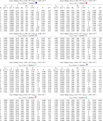
Experimental conditions.

Flow was supplied to the test section from a 4000 L cylindrical tank. Water was drawn from the tank to two variable speed pumps operating in parallel and then sent to a flow conditioning section consisting of a diffuser containing perforated plates, a honeycomb, three screens and a three-dimensional contraction. Following the contraction was a second honeycomb and two additional screens. The test section followed these screens. The free stream turbulence level was 0.3 %. Water exited the test section through a perforated plate emptying into the cylindrical tank. The test fluid was filtered and deaerated water. A chiller was used to keep the water temperature constant to within 0.5 °C during all tests.
Boundary layer velocity measurements were obtained with a TSI FSA3500 two-component laser Doppler velocimeter. A four-beam fibre optic probe was used to collect data in backscatter mode. The beams entered the test section through one of the sidewalls. A custom designed beam displacer was added to the probe to shift one of the four beams, resulting in three co-planar beams that were aligned parallel to the test wall. Additionally, a 2.6 : 1 beam expander was located at the exit of the probe to reduce the size of the measurement volume. The resulting probe volume diameter (d) was 45 μm and the probe volume length (l) was 340 μm. The corresponding diameter and length in viscous units were d + ≤ 7.4 and l + ≤ 56. The flow was seeded with 2 μm diameter silver coated glass spheres. The data were collected in coincidence mode. For each velocity profile, the laser Doppler velocimetry (LDV) probe was traversed to 43 locations within the boundary layer using an Isel three-axis traverse with a resolution of ±6.25 μm in all directions. Data were acquired at each location for 10 000 large eddy turnover times, δ/U∞, where U∞ is the local free stream velocity. Due to the varying data rate with distance from the wall, the number of realizations typically varied from roughly 40 000 near the wall, to approximately 80 000 in the free stream.
The uncertainty in the mean streamwise velocity was 0.5 % of the free stream velocity. The 95 % confidence interval uncertainty in the turbulence quantities was determined using the bootstrapping method and ranged from 1 % to 4 % in the Reynolds stresses. Uncertainties in triple products ranged from 5 % to 30 % depending on the quantity and the location in the boundary layer. More details of the uncertainty estimates are reported by Volino & Schultz (Reference Volino and Schultz2022).
The friction velocity and skin friction coefficient,  ${C_f}/2 = {({u_\tau }/{U_\infty })^2}$, were determined for each velocity profile using the method described by Volino & Schultz (Reference Volino and Schultz2018) with an uncertainty in uτ of 3 %. The method is based on the streamwise momentum equation and uses the measured mean streamwise velocity and Reynolds shear stress profiles. The Clauser chart method, which is based on fitting the mean profile to the law of the wall, may not be applicable in all of the present cases because the strong pressure gradients may cause deviation from the standard log law. In ZPG regions, uτ from the present method and the Clauser chart method agreed to within 3 %. The location of y = 0 was found by shifting the data in the y direction so that the data in the range recommended by Squire et al. (Reference Squire, Morrill-Winter, Hutchins, Schultz, Klewicki and Marusic2016) for ZPG boundary layers,
 $3.4\sqrt {{\delta ^ + }} < {y^ + } < 0.19{\delta ^ + }$, agreed with the log law as closely as possible. This method of finding y = 0 presumes that a log region exists and that the ZPG slope is preserved. There is no way of checking this assumption using existing data, but it appears to be a reasonable approximation based on the response of smooth-wall boundary layers to pressure gradients. Since the y shift is of the order of the physical roughness height, which is much smaller than the boundary layer thickness, it has little effect on the appearance of the results in the outer boundary layer. The determination of ΔU + is based on the downward shift of the data below the smooth-wall log law with κ = 0.384 and B = 4.2. As explained by Volino & Schultz (Reference Volino and Schultz2022), the uncertainty in uτ results in a 5 % uncertainty in ΔU + for ZPG cases, which causes a 15 % uncertainty in ks found using (1.2). For non-ZPG cases, the appropriate value of B to use in finding ΔU + is not obvious. Smooth-wall experiments and DNS such as those of Spalart (Reference Spalart1986), Aubertine & Eaton (Reference Aubertine and Eaton2005) and Volino (Reference Volino2020), indicate that B does not change noticeably for APG cases or with a mild FPG, but it may go up by as much as approximately 1.5 with a strong FPG. For consistency and because of the lack of certainty in what might be a more appropriate B for non-ZPG rough-wall cases, B = 4.2 is used to find ΔU + for all of the present cases. It is recognized that other choices for B are possible and these could increase the value reported for ΔU + by as much as 1.5 for the strong FPG cases.
Velocity field measurements were made using planar particle image velocimetry (PIV) at the same streamwise locations as the LDV profiles. At each location, a streamwise-wall normal (x–y) plane was acquired at the spanwise centreline of the test section, and streamwise-spanwise (x–z) planes were acquired at y/δ = 0.15 and 0.4. The flow was seeded with the same particles used in the LDV measurements. For each plane, 1000 image pairs were acquired using a CCD camera with a 3320 × 2496 pixel array. Velocity vectors were obtained with TSI Insight 4G software using 32 pixel square windows with 50 % overlap. The field of view was 80 mm × 61 mm in the x–z plane, and in the x–y plane was varied from 50 mm × 38 mm to 82 mm × 62 mm depending on the local boundary layer thickness.
2.1. Test cases
All test cases included a 0.6 m long ZPG development region at the inlet of the test section. The first measurement station was near the end of this section. The top wall of the test section was slightly diverging in this region to account for the growth of the boundary layers on all four walls.
The following section was set for an FPG from x = 0.6 m to 1.1 m, where x is the streamwise distance downstream of the trip. The FPG had a constant acceleration parameter:
 \begin{equation}K = \frac{\nu }{{U_\infty ^2}}\frac{{\textrm{d}{U_\infty }}}{{\textrm{d}\kern0.06em x}}.\end{equation}
On a smooth wall, a constant K FPG is a sink flow, which will reach equilibrium in all dimensionless quantities if given sufficiently long to develop. On a wall with uniform roughness, equilibrium will not be reached since δ/ks will, at some point, begin to decrease continuously in the streamwise direction.
The FPG region was followed by a ZPG recovery region extending from x = 1.1 m to 1.6 m. This was followed by a constant K APG region. The K value in the APG was set to half the magnitude of the upstream FPG in each case. A free stream core was maintained between the test-wall and upper-wall boundary layers at all measurement locations. As explained by Bobke et al. (Reference Bobke, Vinuesa, Orlu and Schlatter2017) based on the work of Mellor & Gibson (Reference Mellor and Gibson1966), near equilibrium, in which the mean velocity is streamwise invariant in defect coordinates, is possible in some APG cases when the pressure gradient parameter
 \begin{equation}\beta = \frac{{{\delta ^\ast }}}{{\rho u_\tau ^2}}\frac{{\textrm{d}P}}{{\textrm{d}\kern0.06em x}} = R{e_{{\delta ^\ast }}}\frac{{ - K}}{{{C_f}/2}}\end{equation}
(where δ* is the displacement thickness and P is pressure) is constant. In the present cases, β continuously increased in the streamwise direction, so equilibrium was not achieved or approached.
Three positions of the upper wall were used, as shown in figure 1. Three different inlet velocities, U∞o, = 0.5, 1 and 2 m s−1, were used, resulting in eight experimental cases with K values shown in table 2. The highest K was 2 × 10⁻⁶, which is strong enough to significantly reduce the turbulence in the boundary layer, but below the threshold needed to produce relaminarization in a smooth-wall case. The largest negative K values caused the rough-wall boundary layer to approach, but not reach, separation. The K values reported in table 2 were determined by fitting the measured U∞ at each station to the integral of (2.1). The K for each case was then used to compute the expected U∞ at each station, and these computed values agreed with the measured U∞ to within 0.5 % at all stations. This indicates that K is essentially constant in the FPG and APG regions. The momentum thickness Reynolds number, Reθ, dropped slightly with streamwise distance through the FPG region with the aggressive setting of the upper wall, and rose with the weaker pressure gradients, although more slowly than with a ZPG. The three positions of the upper wall will be referred to below as ramps 1, 2 and 3 for the strong, moderate and mild pressure gradients, respectively.
The twelve streamwise stations used for measurements are shown in table 3 and figure 1. Station 1 was near the end of the ZPG entry region, stations 2–6 were in the FPG region, stations 7–9 spanned the ZPG recovery and stations 10–12 were in the APG region. Table 2 gives boundary layer parameters for all cases including the friction Reynolds number,  $R{e_\tau } = {u_\tau }\delta /\nu$, and the shape factor, H = δ*/θ. The wake strength,
 $\varPi $, is defined as the difference between the measured velocity in wall coordinates at δ and the log law
 \begin{equation}\varPi = \frac{\kappa }{2}\left( {0.99U_\infty^ +- \left( {\frac{1}{\kappa }\ln {\delta^ + } + B - \Delta {U^ + }} \right)} \right).\end{equation}
In addition to the non-ZPG cases, data were also acquired for comparison cases with the same inlet free stream velocities and a ZPG along the entire test section. These cases are presented by Volino & Schultz (Reference Volino and Schultz2022).
Measurement station streamwise locations.

3. Results
3.1. Reynolds number independence
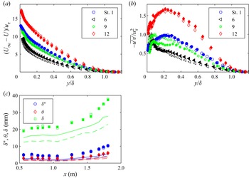
As noted by Pullin, Hutchins & Chung (Reference Pullin, Hutchins and Chung2017), δ is not a function of Reynolds number at a fixed downstream location in a fully rough ZPG turbulent boundary layer. The boundary layer will grow in the streamwise direction but, at any fixed streamwise location, δ will not vary if the free stream velocity is changed. This is unlike the smooth-wall case where δ varies inversely with U∞ due to viscous effects. In the rough-wall case, the skin friction coefficient and all dimensionless flow quantities normalized using uτ and δ are also invariant with U∞. Although one might expect the same invariance in non-ZPG cases, there is limited direct evidence in the literature to confirm this. The present results do confirm it in all cases. Figure 2 shows profiles of the mean velocity in defect coordinates, the Reynolds shear stress and boundary layer thicknesses from cases 3 and 5 at stations 1, 6, 9 and 12, which correspond to the ends of the initial ZPG, FPG, ZPG recovery and APG regions, respectively. Cases 3 and 5 have the same test section geometry with the moderate pressure gradient. The open symbols in the figure correspond to the U∞o = 0.5 m s−1 case, and the filled symbols to the U∞o = 2 m s−1 case. There is considerable variation in the quantities in the streamwise direction, but at each station, there is essentially no difference between the case 3 and 5 results. The same is true for all other turbulence quantities and β. The largest variation with Reynolds number visible is in the  $- \overline {u^{\prime}v^{\prime}} $ profile at station 9 in figure 2(b). Even in this case, the difference between the U∞o = 0.5 m s−1 and U∞o = 2 m s−1 profiles is only slightly outside the uncertainty bands. The boundary layer thicknesses in figure 2(c) show Reynolds number independence for the rough-wall cases. Also shown for comparison are the corresponding smooth-wall cases. As expected, the boundary layer is thinner on the smooth wall. There is also a clear variation with Reynolds number, with the boundary layer thicknesses lower for the high U∞o case. The Reynolds number independence in figure 2 is also seen when comparing cases 1 and 2 with the strong pressure gradient, and when comparing cases 6, 7 and 8 with the mild pressure gradient. It is interesting to note that the agreement between cases includes those with U∞o = 0.5 m s−1, which resulted in
 $k_s^ + < 80$ (i.e. below the cutoff for fully rough conditions) at all locations and below 30 at some locations. Since the results do not vary with the free stream velocity, the focus below is on cases 2, 4 and 7 with U∞o = 1 m s−1.
Data from moderate ramp cases showing Reynolds number independence: (a) mean velocity profiles at stations (St.) 1, 6, 9 and 12 at end of initial ZPG, FPG, ZPG recovery and APG regions; (b) Reynolds shear stress profiles; (c) boundary layer thicknesses. Open symbols from the U∞,o = 0.5 m s−1 case, solid symbols from the U∞,o = 2 m s−1 case. Lines show values for corresponding smooth-wall cases with colours corresponding to quantities in the legend, solid lines for the U∞,o = 0.5 m s−1 case, dashed lines for U∞,o = 2 m s−1 case.

3.2. Mean velocity profiles
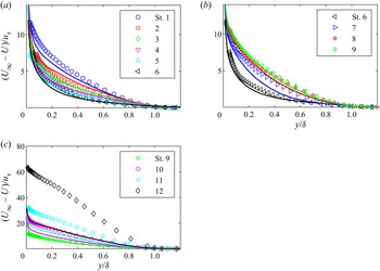
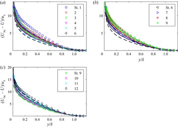
Mean velocity profiles in defect coordinates are shown in figure 3 for case 2 with ramp 1. The symbols in each plot correspond to the 12 streamwise stations of the present rough-wall case. The solid lines correspond to the stations of the corresponding smooth-wall case with ramp 1 from Volino (Reference Volino2020), with the colour of the symbol and line matching at each station. The FPG region is shown in figure 3(a). The acceleration causes a drop in the profiles. There is good agreement between the rough- and smooth-wall cases at each station, with the rough-wall case appearing to proceed slightly faster through the non-equilibrium, in agreement with the findings of Yuan & Piomelli (Reference Yuan and Piomelli2015). The β values in the FPG are close for the two cases, varying from −1.15 to −0.7 in the smooth-wall case and from −0.84 to −0.62 in the rough-wall case. The rough-wall profiles at stations 5 and 6 are essentially the same, suggesting that although a true equilibrium cannot be reached with a constant K on a wall with uniform roughness, δ/ks may remain large enough in the present case so that an approximate or local equilibrium is achieved.
Mean streamwise velocity profiles in defect coordinates for case 2, ramp 1: (a) St. 1–6; (b) St. 6–9; (c) St. 9–12. Symbols for rough-wall case, lines for smooth-wall case of Volino (Reference Volino2020). Symbol and line colour match at each station.

The agreement of the smooth- and rough-wall profiles is also good in the ZPG recovery shown in figure 3(b). Again, the rough-wall case proceeds somewhat faster toward the new equilibrium, but by the end of the recovery region at station 9, there is good similarity between the rough and smooth cases and good agreement with canonical ZPG results, indicating that the recovery from the FPG is complete. In the APG region shown in figure 3(c), the similarity is lost. The APG causes the profiles to rise above the ZPG result, and this rise is much higher for the rough-wall case. The boundary layer grows much faster on the rough wall, resulting in a much larger velocity deficit and a much lower friction velocity as the boundary layer approaches separation. The dimensionless pressure gradient history is very different for the rough- and smooth-wall cases in the APG, with β an order of magnitude higher on the rough wall by station 12.
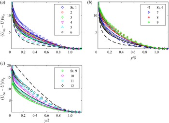
Figure 4 shows the rough-wall case 4 profiles with the moderate pressure gradient of ramp 2 in the same format as figure 3. For comparison, the corresponding ramp 2 smooth-wall case is shown with solid lines, and the ramp 1 smooth-wall case of figure 3 is shown with dashed lines. The extent of the change in the streamwise direction is lower in figure 4 than in figure 3 because the pressure gradient is weaker, but the trends are the same. In the FPG and ZPG recovery, there is similarity between the rough-wall case and the smooth-wall case with the same ramp, but the rough-wall case appears to respond slightly more quickly to the changes in pressure gradient and reach a new equilibrium in a shorter distance. In the FPG region, the β values for the rough-wall case are nearly equal those of the smooth-wall case with the same ramp. In the APG region, the rough-wall profiles are above the smooth-wall ramp 2 profiles, and the β values for the rough-wall case are approximately 70 % higher than in the ramp 2 smooth-wall case. The rough wall profiles in figure 4(c) match more closely with those of the ramp 1 smooth-wall case. The β values in these two cases agreed to within 8 % at stations 11 and 12. This suggests that if the β history for a rough- and smooth-wall case were matched, as opposed to matching the dimensional pressure gradient, then similarity might be achieved.
Mean streamwise velocity profiles in defect coordinates for case 4, ramp 2: (a) St. 1–6; (b) St. 6–9; (c) St. 9–12. Symbols for rough-wall case; solid lines for smooth-wall ramp 2 case; dashed lines for smooth-wall ramp 1 case. Symbol and line colour match at each station.

The ramp 3 mild pressure gradient case is shown in figure 5 in the same format as figure 4. The ramp 2 and 3 smooth-wall cases are shown for comparison. The effect of the pressure gradient on the profiles is weak, but the trends are consistent with those in the cases above. In the FPG and ZPG regions, in agreement with the cases above, the smooth and rough cases with the same ramp exhibit good similarity at each station and the β values for the two cases are approximately equal. In the APG region, β values for the rough-wall case fall between those of the ramp 2 and 3 smooth-wall cases. The rough-wall profiles agree better with those of the smooth-wall ramp 2 case, but the differences among all of the profiles of figure 5(c) are small.
Mean streamwise velocity profiles in defect coordinates for case 7, ramp 3: (a) St. 1–6; (b) St. 6–9; (c) St. 9–12. Symbols for rough-wall case; solid lines for smooth-wall ramp 3 case; dashed lines for smooth-wall ramp 2 case. Symbol and line colour match at each station.

To quantify the rate at which the profiles in figures 3–5 approach or depart from equilibrium, figure 6 show the difference between the measured defect velocity and the corresponding defect velocity under ZPG conditions for the same wall. As was done by Volino (Reference Volino2020), the difference is taken at y/δ = 0.4 and is shown as a function of dimensionless streamwise location. As explained by Volino (Reference Volino2020), the location y/δ = 0.4 was chosen as approximately the centre of the region where the change in the profiles was most pronounced. The streamwise coordinate in the FPG region is (x − xf)/L, where xf is the location at the start of the FPG and  $L = \nu /({K_{FPG}}{U_{\infty f}})$ is the sink flow length, with U∞f the free stream velocity at the start of the FPG. Results from the FPG region for all of the smooth- and rough-wall cases are shown in figure 6(a). All cases follow the same general trend. In the strong and moderate ramp cases, the change in the velocity defect appears to approach the same equilibrium values in the smooth- and rough-wall cases, but it is reached approximately 20 % faster in the rough-wall cases.
Difference in  $A = {(({U_\infty } - U)/{U_\infty })_{ZPG}} - (({U_\infty } - U)/{U_\infty })$ between ZPG and non-ZPG mean velocity defect profiles at y/δ = 0.4. (a) FPG St. 1–6, (b) ZPG St. 6–9, (c) APG St. 9–12, (d) all stations as a function of β, (e) all stations as a function of G. Symbols for rough-wall cases as in table 2, symbols for smooth-wall cases match shapes and filling of table 2 with cyan, magenta and black for U∞,o = 0.5 m s−1, U∞,o = 1 m s−1 and U∞,o = 2 m s−1, respectively.

Figure 6(b) shows results from the ZPG recovery stations. As was done by Volino (Reference Volino2020), the sink flow length is again used to normalize the streamwise coordinate (x − xr)/L, where xr is the location at the start of the ZPG, and an offset  ${x_s}/L = 0.7({x_r} - {x_f})/L$ is applied to account for the cases with stronger pressure gradients (lower L) having departed more from ZPG conditions in the FPG, thereby requiring a longer recovery distance to return to canonical ZPG behaviour. The constant 0.7 was determined empirically to collapse the data by Volino (Reference Volino2020). All cases follow the same trend in the ZPG recovery, with all cases returning to canonical ZPG conditions, and no obvious difference between the rough- and smooth-wall cases.
Adverse pressure gradient region results are shown in figure 6(c). The streamwise coordinate is  $(x - {x_a})/{L_a}$, where xa is the location at the start of the APG and
 ${L_a} = \nu /({K_{APG}}{U_{\infty a}})$, with U∞a the free stream velocity at the start of the APG. As discussed above, the results in this region do not collapse, with the rough-wall cases departing much more strongly from ZPG conditions. Figure 6(d) shows the results from all regions as a function of the Clauser pressure gradient parameter β. All cases fall along the same curve and the larger differences from ZPG conditions on the rough wall, particularly in the APG region, are shown to be a function of the higher β on the rough wall. Figure 6(e) shows a somewhat better collapse when the results are shown as a function of the Clauser shape factor,
 $G = ({U_\infty }/{u_\tau })(H - 1)/H$. The significance of G with respect to equilibrium will be discussed further below.
Various quantities can be extracted from the mean profiles and some of these are considered next. Figure 7 shows the friction Reynolds number, Reτ, as a function of Reθ for all stations and cases. A linear fit to the ZPG data of Volino & Schultz (Reference Volino and Schultz2022) is included for reference. The APG causes Reτ to fall below the ZPG line. If an empirical correction of (1 + β/12) is applied to Reτ, as shown in figure 7(b), better agreement with the ZPG line is achieved. There are two points that are clearly overcorrected above the ZPG line. These points are from the most downstream station of the ramp 1 cases, where β is very high and the boundary layer is near separation. The rough wall results in figure 7 are similar to those of the smooth-wall cases of Volino (Reference Volino2020), with the only differences being that the slope of the ZPG line was approximately 20 % higher and the coefficient on β in the correction term approximately 20 % lower in the rough-wall case.
Friction Reynolds number as function of momentum thickness Reynolds number for rough-wall cases, (a) uncorrected results, (b) correction using Clauser pressure gradient parameter applied. Symbols as in figure 6 for non-ZPG cases, black filled stars are for ZPG cases of Volino & Schultz (Reference Volino and Schultz2022). Solid black line is fit to ZPG results from Volino & Schultz (Reference Volino and Schultz2022).

The skin friction coefficients for all of the rough- and smooth-wall cases are shown as a function of θ/yo in figure 8, where yo is the roughness length:
 \begin{equation}{y_o} = \frac{\nu }{{{u_\tau }}}\,{\textrm{e}^{\kappa (\Delta {U^ + } - B)}},\end{equation}
which is the distance from the wall where the log region of the mean velocity profile extrapolates to zero. For the smooth wall, ΔU + = 0 and  ${y_o} = \nu /{u_\tau }\,{\textrm{e}^{ - \kappa B}} = 0.2\nu /{u_\tau }$. The curve in the figure is a theoretical expression from Castro (Reference Castro2007) for ZPG conditions:
 \begin{equation}\frac{\theta }{{{y_o}}} = \frac{{\sqrt {2/{C_f}} - I}}{{2/{C_f}}}\,{\textrm{e}^{\kappa \left( {\sqrt {2/{C_f}} - {K_c}} \right)}},\end{equation}
where  ${K_c} = 2{\varPi _c}/\kappa - (1/\kappa )\ln ((1 + {\varPi _c})/\kappa )$ and I are constants. Typical values from Castro (Reference Castro2007) of I = 7 and Πc = 0.7 are used, resulting in Kc = −0.228. The ZPG data from both the smooth- and rough-wall cases agree well with the theoretical curve, but the APG results fall below it and the FPG results are above. Kays & Crawford (Reference Kays and Crawford1980) suggest an empirical correction to Cf of (1 + β/5). For the present results, (1 + β/6) provided a somewhat better fit and this is shown in figure 8(b). Although the correction was originally proposed for equilibrium flows with constant β, it works well for most of the present cases, which are not in equilibrium. This may be due to the near-wall flow, which has the most direct influence on Cf, adjusting more rapidly to changes in the pressure gradient and reaching equilibrium faster than the rest of the boundary layer. Volino (Reference Volino2020) showed a more rapid response to changes in the pressure gradient closer to the wall in turbulence spectra results for the smooth-wall cases, and further evidence of this for the present cases will be shown below using spatial correlations. At the most downstream station of the APG in the ramp 1 cases, (1 + β/6) produces an overcorrection. This may be due to the flow being in the transitionally rough regime and/or it being farther from equilibrium as the boundary layer approaches separation.
Skin friction coefficient as a function of momentum thickness over roughness length: (a) uncorrected results; (b) corrected using Clauser pressure gradient parameter. Symbols for non-ZPG cases as in figure 6. Black filled stars are for ZPG cases. Solid black line is ZPG correlation from Castro (Reference Castro2007).

Figure 9 shows the shape factor, H, as a function of θ/yo. A theoretical curve for ZPG boundary layers from Castro (Reference Castro2007),
 \begin{equation}H = {\left( {1 - I\sqrt {{C_f}/2} } \right)^{ - 1}},\end{equation}
is also included. The ZPG results for both the smooth- and rough-wall cases agree well with the theoretical curve, as also shown by Volino & Schultz (Reference Volino and Schultz2022). The APG results lie above the curve as the boundary layer proceeds toward separation, causing H to increase. A correction, similar to that used with Cf in figure 8, is applied in figure 9(b) and results in a better collapse of the data.
Shape factor, H, as a function of momentum thickness divided by roughness length, as done by Castro (Reference Castro2007): (a) uncorrected results; (b) corrected using Clauser pressure gradient parameter. Symbols as in figure 8.

The Clauser shape factor, G, can be used to evaluate the extent of the departure of a boundary layer from equilibrium. It is shown in figure 10 as a function of β along with a curve derived from the equilibrium results presented by Mellor & Gibson (Reference Mellor and Gibson1966). The APG results depart significantly from the equilibrium curve in the ramp 1 cases on both the smooth and rough walls, with the data points lying approximately 20 % below the equilibrium curve. The ramp 2 APG results lie approximately 8 % below the equilibrium curve and for ramp 3, the data match the equilibrium curve. In the FPG region, the results lie above the equilibrium curve and approach the curve as the flow proceeds in the streamwise direction. In the strong and moderate pressure gradient cases, the FPG results are noticeably closer to equilibrium on the rough wall than on the smooth wall, in agreement with the observation in figures 3, 4 and 6 that the rough-wall cases appeared to proceed towards a new equilibrium more rapidly after a change in pressure gradient, possibly due to the increased turbulence and mixing induced by the roughness.
Clauser shape factor as a function of Clauser pressure gradient parameter, (b) and (c) expanded views of panel (a). Symbols as in figure 6. Solid line is equilibrium condition from Mellor & Gibson (Reference Mellor and Gibson1966).

The equivalent sandgrain roughness height was determined for each profile using (1.2). The average obtained from all profiles with  $k_s^ + > 80$ was 2.3 mm. Figure 11(a) shows ΔU + as a function of
 $k_s^ +$, with
 $k_s^ +$ computed for each profile using the average ks = 2.3 mm. The general trend of the data agrees with (1.2), but there is considerable scatter. The dashed lines in the figure show (1.2) shifted relative to the data for ks values of 1.2 mm and 3.5 mm, indicating the variability in ks found from individual profiles. Volino & Schultz (Reference Volino and Schultz2022) found an average ks of 1.7 mm for the same surface considering only the ZPG case data. They also noted that the ks values computed from (1.2) generally tended to be higher for profiles with lower δ, and suggested that as δ/ks became large, ks tended toward a value of ksh = 1.3 mm. In figure 11(b), ks/ksh is shown as a function of δ/ksh. Results from profiles with
 $k_s^ + < 80$ are not included. Also excluded are results from the FPG region of the ramp 1 cases, in which changes in the log law explained above raise the uncertainty in ΔU +. The scatter in figure 11(b) makes any firm conclusion impossible, but there is a general trend of higher ks when δ is small. As explained by Volino & Schultz (Reference Volino and Schultz2022), this may be due to a lack of separation between the inner and outer scales of the flow when δ is small, and suggests that (1.2) may be missing a dependence on δ/ks. The data were examined to consider the possibility that ks might depend on the pressure gradient. No obvious dependence on pressure gradient was observed, but there was some tendency for higher ks at FPG stations and lower ks at APG stations. The boundary layer thickness is reduced by an FPG and increases with an APG, however, so any tendencies in ks observed with the pressure gradient can also be explained in terms of a δ/ks dependency, which was also observed in ZPG cases.
Equivalent sandgrain roughness height: (a) roughness function as function of  $k_s^ +$ with ks = 2.3 mm assumed; (b) locally determined ks as function of δ with both normalized on estimated ksh at high δ/ks. Solid line is (1.2), dashed lines are displaced from solid line to correspond to ks = 3.5 mm (upper) and 1.2 mm (lower). Symbols as in figure 8.

3.3. Reynolds stresses
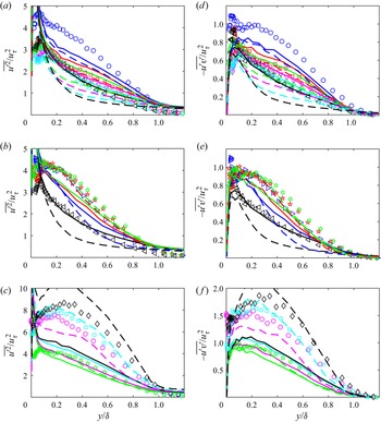
The boundary layer turbulence is considered next. Figure 12 shows profiles of the streamwise component of the Reynolds normal stress,  $\overline {{{u^{\prime}}^2}} $, and the Reynolds shear stress,
 $- \overline {u^{\prime}v^{\prime}} $, for the ramp 1 case of figure 3. The smooth-wall peak in
 $\overline {{{u^{\prime}}^2}} $ at y + = 15, which is due to viscous shear near the wall, is absent in the rough-wall case, as expected. Outside the roughness sublayer, there is similarity in both
 $\overline {{{u^{\prime}}^2}} $ and
 $- \overline {u^{\prime}v^{\prime}} $ between the rough- and smooth-wall cases in the FPG and ZPG recovery regions. As with the mean velocity, the rough-wall case proceeds more rapidly towards a new equilibrium after each change in the pressure gradient. In the APG region, the similarity is lost and the rough-wall values are an order of magnitude higher than the smooth. The high peaks in the APG region are caused primarily by the drop in the normalizing quantity, uτ. The dimensional values of
 $\overline {{{u^{\prime}}^2}} $ and
 $- \overline {u^{\prime}v^{\prime}} $, in both the rough- and smooth-wall cases, do not change significantly in the outer region in response to the APG. Close to the wall in the APG region, the dimensional Reynolds stresses actually drop in the streamwise direction due to the reduction in the mean velocity gradient, from which they are produced. The wall-normal component of the Reynolds normal stress,
 $\overline {{{v^{\prime}}^2}} $, is not shown, but behaves in all ways very similarly to
 $- \overline {u^{\prime}v^{\prime}} $. Figure 13 shows the
 $\overline {{{u^{\prime}}^2}} $ and
 $- \overline {u^{\prime}v^{\prime}} $ results for the ramp 2 case of figure 4. As with the mean velocity, there is again similarity between the ramp 2 rough- and smooth-wall cases in the FPG and ZPG regions, with the rough-wall case proceeding towards a new equilibrium more quickly. In the APG region, the rough-wall profiles lie well above the ramp 2 smooth-wall profiles, but are in better agreement with the ramp 1 profiles.
Reynolds stress profiles for case 2, ramp 1: (a)  $\overline {{{u^{\prime}}^2}} $, St. 1–6; (b)
 $\overline {{{u^{\prime}}^2}} $, St. 6–9; (c)
 $\overline {{{u^{\prime}}^2}} $, St. 9–12; (d)
 $- \overline {u^{\prime}v^{\prime}} $, St. 1–6; (e)
 $- \overline {u^{\prime}v^{\prime}} $, St. 6–9; (f)
 $- \overline {u^{\prime}v^{\prime}} $, St. 9–12. Symbols as in figure 3.

Reynolds stress profiles for case 4, ramp 2: (a)  $\overline {{{u^{\prime}}^2}} $, St. 1–6; (b)
 $\overline {{{u^{\prime}}^2}} $, St. 6–9; (c)
 $\overline {{{u^{\prime}}^2}} $, St. 9–12; (d)
 $- \overline {u^{\prime}v^{\prime}} $, St. 1–6; (e)
 $- \overline {u^{\prime}v^{\prime}} $, St. 6–9; (f)
 $- \overline {u^{\prime}v^{\prime}} $, St. 9–12. Symbols as in figure 4.

The extent of the departure of the  $- \overline {u^{\prime}v^{\prime}} $ profiles from ZPG conditions is shown for all cases in figure 14 in the format of figure 6. As with the mean velocity, the smooth- and rough-wall cases follow the same trends in the FPG and ZPG regions, but the rough-wall cases tend to reach a plateau quicker, particularly with the stronger pressure gradient. In the APG regions, there are large differences between the rough- and smooth-wall results. Figures 14(d) and 14(e) show the difference from the ZPG case as functions of β and G, respectively. As with the mean velocity, there is agreement between all cases. Equivalent results (not shown) were seen for the
 $\overline {{{u^{\prime}}^2}} $ data.
Difference in  $A = \; - \overline {u^{\prime}v^{\prime}} /u_\tau ^2$ between ZPG and non-ZPG Reynolds shear stress profiles at y/δ = 0.4: (a) FPG St. 1–6; (b) ZPG St. 6–9; (c) APG St. 9–12; (d) all stations as function of β; (e) all stations as function of G. Symbols as in figure 6.

Quadrant analysis (Willmarth & Lu Reference Willmarth and Lu1972) was used to further examine the effect of the pressure gradient on the Reynolds shear stress. On the smooth wall, Volino (Reference Volino2020) found that within each quadrant, the response of the  $- \overline {u^{\prime}v^{\prime}} $ profiles was essentially the same as for the composite
 $- \overline {u^{\prime}v^{\prime}} $. As expected, and in agreement with ZPG results, quadrants 2 (Q2, ejections, u′ < 0, v′ > 0) and 4 (Q4, sweeps, u′ > 0, v′ < 0) were most significant. At the y location where the Reynolds shear stress was largest, approximately twice as many events and four times the contribution to the Reynolds shear stress occurred in quadrants 2 and 4 than in quadrants 1 and 3, respectively. The present rough-wall cases exhibit approximately the same behaviour. The pressure gradient changes the relative contributions of Q2 to Q4, and profiles of the ratio of these contributions are shown in figure 15 for the ramp 1 and ramp 2 rough- and smooth-wall cases. Also shown for comparison is a profile from a rough-wall ZPG case. In the ZPG cases, the profiles were invariant in the streamwise direction and changed only slightly with the free stream velocity. For the ZPG cases, the ratio rises from the wall to approximately 1.2 at y/δ = 0.07. The ratio remains at 1.2 to y/δ = 0.4. For locations very near the wall, there is little fluid even closer from which ejections can originate, so Q2 contributions are low. Farther out, Q2 and Q4 come more into balance and the ratio is near one. Beyond y/δ = 0.4, the ratio rises to a peak of approximately 2.4 near the edge of the boundary layer as ejections remain significant but the intensity of sweeps decreases as the free stream is approached. Beyond y/δ = 1, the ratio drops towards 1.0 as the turbulence becomes uncorrelated in the free stream and u′v′ has the same magnitude in all four quadrants. For smooth-wall ZPG cases, Volino (Reference Volino2020) saw a slight drop in the ratio from a peak of 1.2 at y/δ = 0.07 to 1.1 between y/δ = 0.07 and 0.4, and the outer peak magnitude at the edge of the boundary layer was approximately 2.2. Other than these differences, the rough- and smooth-wall ZPG cases are similar. In all of the cases in figure 15, the peak near the edge of the boundary layer is lower for the smooth-wall cases. The reason for this is not clear, but it is consistent for all stations of both the ramp 1 and ramp 2 cases. Nearer the wall, there is better agreement between the rough- and smooth-wall cases at station 1. For the ramp 1 cases in figure 15(a–c), the Q2/Q4 ratio rises in the middle of the boundary layer in the FPG region to approximately 1.6. The same behaviour is seen in the smooth-wall case, but the magnitude of the increase is lower for the smooth wall, particularly near the end of the FPG region. For both cases, the rise in the ratio can be attributed to the acceleration straining the turbulence in the outer flow, which reduced the Reynolds stresses as shown in figure 12 and the effect of sweeps. Ejections are still generated due to the high mean shear near the wall, whether due to viscous effects in the smooth-wall cases or the roughness in the present cases. The result is the rising Q2/Q4 ratio. Near the edge of the boundary layer, the FPG reduces the effect of both sweeps and ejections, causing the outer peak to drop. For ejections originating very near the wall, within the roughness sublayer, there may be a difference in the mechanism by which they are generated in the rough- and smooth-wall cases. While the FPG may have some effect in damping the turbulence generated by viscous effects close to the wall, it may not have the same effect on ejections caused by roughness elements. As these ejections move outward into the boundary layer, they may explain the higher ratio seen in the rough-wall cases. In the ZPG recovery region, the ratio returns towards the ZPG value and by the end of the recovery, the smooth- and rough-wall cases are in agreement for y/δ < 0.7. In the APG, the mean shear drops near the wall, reducing the near-wall turbulence and the strength of ejections. In the outer flow, the dimensional turbulence quantities do not change rapidly, so sweeps from the outer region become more significant relative to ejections and the Q2/Q4 ratio drops below the ZPG profile. The same drop in the ratio near the wall was seen in the APG region of the smooth-wall case.
Profiles of the ratio of contributions to  $\overline {u^{\prime}v^{\prime}} $ from Q2 and Q4: (a) case 2, St. 1–6; (b) case 2, St. 6–9; (c) case 2, St. 9–12; (d) case 4, St. 1–6; (e) case 4, St. 6–9; (f) case 4, St. 9–12. Symbols from table 2. Solid lines for corresponding smooth-wall cases with line colour matching symbol colour at each station. Dashed line for rough-wall ZPG comparison case.

For the ramp 2 case shown in figure 15(d–f), the same trends are present as in the ramp 1 case, but they are much less pronounced with the moderate pressure gradient. In the ramp 3 case (not shown), the weak pressure gradient results in no discernible variation from the ZPG profile.
3.4. Turbulence budget terms
Some of the terms in the budget equations of the Reynolds stresses, as presented for example by Reynolds (Reference Reynolds1976), were quantified in the present experiments, and are useful for understanding the development of the turbulence. The triple products of the turbulent fluctuations,  $\overline {{{u^{\prime}}^3}} $,
 $\overline {{{v^{\prime}}^3}} $,
 $\overline {{{u^{\prime}}^2}v^{\prime}} $ and
 $\overline {u^{\prime}{{v^{\prime}}^2}} $, are related to the transport of the Reynolds stresses. Volino (Reference Volino2020) described their physical meaning and explained their behaviour in response to changing pressure gradients for the smooth-wall cases. Profiles of
 $\overline {{{u^{\prime}}^2}v^{\prime}} $, which is primarily related to the wall-normal transport of
 $\overline {{{u^{\prime}}^2}} $, are shown in figure 16, with the ramp 1 case in figure 16(a–c). In the smooth-wall profiles, there is a positive peak near the wall that is caused when ejections with positive v′ carry
 ${u^{\prime 2}}$ away from the near wall
 $\overline {{{u^{\prime}}^2}} $ peak. For the rough-wall cases, this
 $\overline {{{u^{\prime}}^2}v^{\prime}} $ peak is absent, because the near wall
 $\overline {{{u^{\prime}}^2}} $ peak is suppressed by the roughness. In the outer region of the boundary layer in the FPG and ZPG recovery regions, there is a broad peak in
 $\overline {{{u^{\prime}}^2}v^{\prime}} $ centred between y/δ = 0.3 and 0.6. This peak is generated by transport of the outer region
 $\overline {{{u^{\prime}}^2}} $ fluctuations, centred at y/δ = 0.2 in figure 12(a,b), towards the free stream by ejections. As these fluctuations are suppressed by the FPG, the corresponding
 $\overline {{{u^{\prime}}^2}v^{\prime}} $ is also suppressed. The transport of outer region
 $\overline {{{u^{\prime}}^2}} $ towards the wall by sweeps (with negative v′) produces the negative
 $\overline {{{u^{\prime}}^2}v^{\prime}} $ closer to the wall in the rough-wall case. The near wall negative
 $\overline {{{u^{\prime}}^2}v^{\prime}} $ does not appear in the smooth-wall case because it is overwhelmed by the effect of the inner smooth-wall
 $\overline {{{u^{\prime}}^2}} $ peak. In the FPG and ZPG recovery regions, there is outer layer similarity between the rough- and smooth-wall cases, but as in the Reynolds stresses, the rough-wall case proceeds to its new equilibrium faster than the smooth-wall case when the pressure gradient is changed. In the APG region shown in figure 16(c), the
 $\overline {{{u^{\prime}}^2}v^{\prime}} $ peak is much higher in the rough-wall case than in the smooth, following the behaviour of
 $\overline {{{u^{\prime}}^2}} $.


Profiles of  $\overline {{{u^{\prime}}^2}v^{\prime}} $ for the ramp 2 case are shown in figure 16(d–f). In the FPG and ZPG regions, the behaviour is essentially the same as with the stronger pressure gradient. In the APG region, the ramp 2 rough-wall case agrees better with the ramp 1 smooth-wall case than the ramp 2 smooth-wall case. This matches the behaviour of the Reynolds stresses for these cases.
The other triple products are not shown, but they were also examined and they exhibited the same similarity between the rough- and smooth-wall cases as  $\overline {{{u^{\prime}}^2}v^{\prime}} $.
The production terms for the Reynolds stresses were determined from the measurements. The production terms for  $\overline {{{u^{\prime}}^2}} $ are
 $- 2\overline {u^{\prime}v^{\prime}} \partial U/\partial y$ and
 $- 2\overline {{{u^{\prime}}^2}} \partial U/\partial x$, as explained by Reynolds (Reference Reynolds1976). The former is the dominant term since the gradient of the mean velocity is much stronger in the wall-normal direction than in the streamwise direction even for the strong pressure gradient cases. Profiles of
 $- 2\overline {u^{\prime}v^{\prime}} \partial U/\partial y$ are shown in figure 17. In the ramp 1 case, the FPG suppresses the production, which is consistent with the lower
 $\overline {{{u^{\prime}}^2}} $ associated with the FPG. There is similarity between the rough- and smooth-wall cases in the FPG region. The similarity continues in the ZPG recovery, where the production term rises. In the APG region, the production is much higher for the rough-wall case, again consistent with the
 $\overline {{{u^{\prime}}^2}} $ profiles. The ramp 2 rough-wall case agrees with the ramp 2 smooth-wall case in the FPG and ZPG regions. In the APG, the ramp 2 rough-wall case agrees better with the ramp 1 smooth-wall case, again consistent with all of the other quantities presented above.
Profiles of  $- 2\overline {u^{\prime}v^{\prime}} \partial U/\partial y$ (production term for
 $\overline {{{u^{\prime}}^2}} $): (a) case 2, St. 1–6; (b) case 2, St. 6–9; (c) case 2, St. 9–12; (d) case 4, St. 1–6; (e) case 4, St. 6–9; (f) case 4, St. 9–12. Symbols and lines for panels (a–c) as in figure 3 and for panels (d–f) as in figure 4.

The production terms for  $- \overline {u^{\prime}v^{\prime}} $ are
 $\overline {{{u^{\prime}}^2}} \partial V/\partial x$,
 $\overline {u^{\prime}v^{\prime}} \partial V/\partial y$,
 $\overline {u^{\prime}v^{\prime}} \partial U/\partial x$ and
 $\overline {{{v^{\prime}}^2}} \partial U/\partial y$. Of these, the last is the dominant term. Profiles of it are not shown, but they were computed and they agreed very closely with the profiles of figure 17.
3.5. Turbulence structure, x–y plane
Two-point correlations were used to examine the effect of the roughness and pressure gradient on the turbulence structure. In the x–y plane, the correlation, as explained by Volino et al. (Reference Volino, Schultz and Flack2007), is defined as
 \begin{equation}{R_{AB}}({y_{ref}}) = \frac{{\overline {A(x,{y_{ref}})B(x + \Delta x,{y_{ref}} + \Delta y)} }}{{{\sigma _A}({y_{ref}}){\sigma _B}({y_{ref}} + \Delta y)}},\end{equation}
where A and B are the quantities of interest at two locations separated in the streamwise and wall-normal directions by Δx and Δy, and σA and σB are the standard deviations of A and B at yref and yref + Δy, respectively. At every yref, the overbar indicates the correlations were averaged among locations with the same Δx and Δy, and then time averaged over the 1000 vector fields acquired. Figure 18 shows contours of the streamwise fluctuating velocity correlation, Ruu, with the correlation centred at yref/δ = 0.4 for all stations of case 2 with ramp 1. The location yref/δ = 0.4 is representative of the middle of the boundary layer. At station 1, the shape and extent of the contours agree with the ZPG results in the literature, such as those of Volino et al. (Reference Volino, Schultz and Flack2007). The correlated region shown can be associated with the extent of a hairpin packet. In the FPG region, the streamwise extent of the contours increases and the inclination angle of the contours with respect to the wall is reduced. In the ZPG recovery region, the trends are reversed. In the APG region, the streamwise extent of the contours is decreased and the inclination angle increases. The reduced inclination angle of the contours in the FPG suggests higher streamwise shearing relative to the ZPG region for a given boundary layer thickness, which agrees with the skin friction coefficients being above the ZPG correlation in figure 8(a). In the APG region, the increased inclination angle of the structures suggests reduced streamwise shearing, in agreement with the lower Cf for the APG locations in figure 8(a). Since the change in inclination angle is directly caused by the pressure gradient, it appears to be reasonable that a correction to Cf based on the pressure gradient parameter, β, might be useful for producing agreement with the ZPG correlation, as shown in figure 8(b). These trends in figure 18 are more clearly illustrated in figure 19, which shows streamwise cuts through the self-correlation point for yref/δ = 0.15 and 0.4. At yref/δ = 0.15, the increase in streamwise extent is visible in the FPG, as is the reversal in the ZPG recovery. In the FPG, the rough- and smooth-wall cases agree well at all stations, providing evidence of similarity. In the ZPG recovery, the streamwise extent of the correlation is somewhat higher for the rough-wall case at each station, but both the rough- and smooth-wall cases show the same trend of decreasing streamwise extent. The streamwise length decreases in the APG region for the rough-wall cases, but remains nearly constant for the smooth wall. This departure from similarity is consistent with that observed in the mean velocity and turbulence statistics in the APG region described above. Farther from the wall, at yref/δ = 0.4, the correlation lengths in the FPG and ZPG recovery regions are higher than at yref/δ = 0.15, and the extent of the changes from ZPG conditions are more pronounced, but the trends in each region are the same. There is no consistent trend regarding the agreement of the smooth- and rough-wall results. They generally agree at all stations, supporting the observations of outer region similarity discussed above. The larger streamwise variation in the results at yref/δ = 0.4 supports the statement made above regarding figure 8, that the near-wall flow will be closer to equilibrium in a changing pressure gradient than the flow farther from the wall. In the APG region, shown in figures 19(c) and 19(f), there is less difference between the results at yref/δ = 0.15 and 0.4. The APG reduces the wall shear, which appears to result in less of an influence of the wall on the near-wall region and less difference between the correlations lengths at the two locations.
Contours of Ruu centred at y/δ = 0.4 for 12 stations of case 2, outermost contour Ruu = 0.1, contour spacing 0.1.

Streamwise slices through self-correlation point of Ruu of case 2 centred at (a–c) yref/δ = 0.15 and (d–f) yref/δ = 0.4: (a,d) St. 1–6; (b,e) St. 6–9; (c,f) St. 9–12. Symbols from table 2, lines for smooth-wall case with line colour matching symbol colour at each station.

To quantify the changes in the correlation for all cases, the inclination angle, θuu, of Ruu was determined, as done by Volino et al. (Reference Volino, Schultz and Flack2007) using a least-squares fit to a line through the points farthest, both upstream and downstream, from the self-correlation peak on each of the Ruu = 0.5, 0.6, 0.7, 0.8 and 0.9 contours. As was done by Volino et al. (Reference Volino, Schultz and Flack2007), the angle was determined for all yref/δ between 0.2 and 0.7 and then averaged. Figure 20 shows the variation of θuu with streamwise location for all smooth- and rough-wall cases. The streamwise coordinate is normalized for each region as in figure 6. Volino et al. (Reference Volino, Schultz and Flack2007) noted that ZPG studies in the literature reported angles ranging from 6° to 20°, so the scatter in the data in figure 20 is to be expected. There are still, however, observable trends. In the FPG, the angle decreases from approximately 12° to approximately 7°, with the lowest angles in the strong pressure gradient cases. In the moderate pressure gradient cases, there is less change in angle and in the weak pressure gradient cases, there is no discernible change from the ZPG angle. In the ZPG recovery, all cases return to approximately 12°. In the APG, the angle continues to rise to approximately 17°. Outer layer similarity is again seen, as there is no clear difference between the rough- and smooth-wall results, except possibly for a slightly higher angle at the end of the APG region in the strong ramp cases. The highest angle for the rough-wall case is 18°, which matches the angle reported by Lee & Sung (Reference Lee and Sung2009) for an APG boundary layer. In their case, the boundary layer was in equilibrium with β = 1.68 and G = 12.4, which are much lower than in some of the present cases. Perhaps the absence of higher θuu in the present cases is due to their not having reached equilibrium. The angle remains nearly constant through the APG in the present strong pressure gradient cases, so another explanation may be that 18° is an upper limit for the angle. Even with a strong APG, the flow in the boundary layer is still moving in the streamwise direction, so the inclination angle of the turbulent structures cannot increase indefinitely. An upper limit for the inclination angle is therefore plausible. Figure 21 shows θuu as a function of β. There is a sharp rise in the angle as β increases from −1 to 1, followed by a more gradual rise as β increases to approximately 6, and then an approximately constant angle as β increases further. There is a line of data points at β = 0 ranging from θuu = 9° to 14° that may be attributed to non-equilibrium behaviour in the ZPG recovery. To possibly account for the departure from equilibrium, figure 21(b) shows θuu as a function of G.
Average inclination angle of Ruu contours as a function of dimensionless streamwise location: (a) St. 1–6; (b) St. 6–9; (c) St. 9–12. Symbols as in figure 6.

Average inclination angle of Ruu contours: (a) as a function of β; (b) as a function of Clauser shape factor, G. Symbols as in figure 6.

The streamwise extent of Ruu, Lxuu, is defined as by Christensen & Wu (Reference Christensen and Wu2005) as twice the distance from the self-correlation peak to the most downstream location on the Ruu = 0.5 contour. It was determined for all yref/δ between 0.2 and 0.7 and then averaged. It is shown in figure 22 as a function of the same dimensionless streamwise locations as in figure 20. As with θuu, there is scatter in the results, but also observable trends. The correlation length increases with the FPG, decreases back towards its original value in the ZPG recovery and decreases slightly in the APG. The changes are largest for the strongest pressure gradient cases and negligible with the mild pressure gradient. There is no obvious difference between the rough- and smooth-wall cases. Volino (Reference Volino2020) attributed the increased streamwise length and decreased inclination of the structures in the FPG to streamwise stretching caused by the acceleration. The decrease in outer region turbulence and the reduced impact of Q4 events noted above would also result is less disturbance from above, so that coherent regions closer to the wall might persist longer in the streamwise direction. The APG would effectively compress the structures instead of stretching them, which would tend to increase the inclination angle. The reduction of Q2 events by an APG might reduce the strength of near-wall structures and make them more susceptible to disruption by sweeps, resulting in lower correlation lengths.
Average streamwise extent of Ruu = 0.5 contour as a function of dimensionless streamwise location: (a) St. 1–6; (b) St. 6–9; (c) St. 9–12. Symbols as in figure 8.

Correlations of the wall-normal component of the turbulence and the signed swirl strength, λ, were also computed, as were cross-correlations between u′, v′ and λ. The swirl strength was defined by Zhou et al. (Reference Zhou, Adrian, Balachandar and Kendall1999) as the imaginary part of the complex eigenvalue of the local velocity gradient tensor. It is closely related to the vorticity resulting from rotation, as opposed to pure shear. It is used here in a two-dimensional form, as explained by Volino, Schultz & Flack (Reference Volino, Schultz and Flack2009) and Hutchins, Hambleton & Marusic (Reference Hutchins, Hambleton and Marusic2005). Prograde swirl, as used by Wu & Christensen (Reference Wu and Christensen2006), is defined as positive in the present figures and refers to vortices rotating in the direction of hairpin vortex heads, which is the direction induced by the mean shear. Contours of Rvv, Ruv, Rλu and Rλv for stations 1, 6, 9 and 12 of the rough-wall strong pressure gradient case are shown in figure 23. The correlations are centred at yref/δ = 0.4, as in figure 18. The Rvv and Rλv correlations show an increase in spatial extent in the FPG region, a reverse in the ZPG recovery and a further reduction in size in the APG. The Rλv contours can be associated with the head of a hairpin vortex (prograde swirl) at the centre of the correlation. Fluid is pulled away from the wall on the upstream side and directed towards the wall on the downstream side. The rough-wall results are similar to the smooth-wall results of Volino (Reference Volino2020) with the exception that the reduction in size of the correlated region is more pronounced for the rough-wall case. This is consistent with all of the results shown above and the larger β in the rough-wall case.
Contours of correlations for case 2: (a) Rvv, innermost contour Rvv = 0.8, contour spacing 0.2; (b) Ruv, innermost contour Rvv = −0.45, contour spacing 0.1; (c) Rλu, outermost contours Rλu = ±0.015, contour spacing 0.04; (d) Rλv, outermost contours Rλv = ±0.01, contour spacing 0.04.

The Ruv and Rλu correlations involve u′ and exhibit inclination angles. In the same manner as θuu, the magnitude of the angle decreases in the FPG, returns to its original value in the ZPG recovery and increases further in the APG. The correlation Rλu can be associated with the head of a hairpin vortex. Fluid is directed downstream above the centre of the correlation and upstream below. The inclination of the line between the positively and negatively correlated region of Rλu decreases with the FPG, and then increases in the recovery and APG regions. The streamwise extent of the correlation, particularly between the correlation centre and the wall, increases with the FPG and then drops in the following regions. There is similarity with the smooth-wall result of Volino (Reference Volino2020), but as with Ruu, the effect of the APG is stronger for the rough-wall case.
The Ruv contours are inclined at a negative angle with respect to the wall, which is consistent with Q2 and Q4 events. The angle, θuv, was quantified using a least-squares fit to define a line though the upstream and downstream points farthest from the centre of the correlation on the −0.3 and −0.35 contours, and is shown in figure 24 as a function of G. The behaviour of θuv is essentially the same as that of θuu in figure 20. With the exception of a few points which appear anomalous in the ramp 2 rough-wall cases, the magnitude of the angle increases with G and for G > 15, reaches a limit of approximately −42°.
Average inclination angle of Ruv contours as a function of Clauser shape factor, G. Symbols as in figure 6.

3.6. Turbulence structure, x–z plane
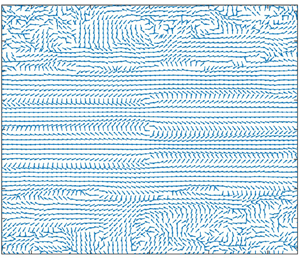
Linear stochastic estimation (LSE) was used in the x–z plane to illustrate the high- and low-speed streaks in the boundary layer, and the legs of hairpin vortices and their spacing, as in studies such as by Hutchins et al. (Reference Hutchins, Hambleton and Marusic2005). The technique, as used here, is explained by Volino et al. (Reference Volino, Schultz and Flack2009), and is similar to that used by Hambleton, Hutchins & Marusic (Reference Hambleton, Hutchins and Marusic2006) and Christensen & Adrian (Reference Christensen and Adrian2001), based on the derivation of Adrian & Moin (Reference Adrian and Moin1988). In LSE, the average velocity field associated with a conditioning event is computed. Whenever the conditioning event occurred, the instantaneous fluctuating velocity field at locations Δx and Δz from the event was identified. Streamwise averaging was then done among all locations with the same Δx and Δz in the field, and then over the 1000 vector fields acquired. Clockwise swirl in the planes shown was used as the conditioning event, as by Volino (Reference Volino2020), to find the average velocity field associated with the leg of a hairpin vortex. Figure 25 shows an example LSE result for case 2 at the end of the ZPG recovery (station 9) in the plane at y/δ = 0.4. Each vector is normalized for presentation by its own magnitude to prevent those closest to the reference point from dominating the field. The arrows, therefore, are all the same length and indicate only direction. The conditioning event is at the origin and appears as a clockwise vortex. Areas of organized vectors indicate correlation with the conditioning event, while regions with random appearing vectors are uncorrelated. The conditioning event can be associated with one leg of a hairpin vortex. Although cane vortices, consisting of only a single leg as opposed to a fully formed hairpin, can occur in the instantaneous flow, in the average that LSE shows, the leg of a hairpin should be accompanied by the opposite leg. This is seen as oppositely rotating vortices spaced at approximately Δz/δ = ±0.5 from the vortex at the centre of the field. Although not as clear in the figure, there is another set of vortices at approximately Δz/δ = ±1 with the same rotation direction as the conditioning vortex. Between the vortices are high- and low-speed streaks of positive and negative u′ induced by the vortices. These streaks extend the full length of the field of view. All the LSE results in the x–z plane were qualitatively similar, but the spanwise spacing of the vortices varied. This spacing is shown as a function of G for all stations of all cases in figure 26 for planes at y/δ = 0.15 and 0.4. The spacing is generally higher at y/δ = 0.4 than closer to the wall. At both locations, the spacing drops with G, which is equivalent to the spacing increasing in the FPG region and decreasing in the APG. As with the streamwise lengths considered above, the changes in spanwise spacing are largest for the strong pressure gradient cases. There is a visible difference between the rough- and smooth-wall cases, with the changes in spacing larger for the smooth-wall case. The size and spacing of the structures decrease as the wall is approached, and the roughness may cause the lower limit of this size to be different than in the smooth-wall case.
LSE conditioned on clockwise swirl events at y/δ = 0.4 for St. 9 of case 2.


Two-point correlations in the x–z plane are defined as
 \begin{equation}{R_{AB}} = \frac{{\overline {A(x,z)B(x + \Delta x,z + \Delta z)} }}{{{\sigma _A}{\sigma _B}}},\end{equation}
where A and B are the quantities of interest at two locations separated by Δx and Δz, and σA and σB are the standard deviations of A and B based on data in the full measurement plane for the 1000 vector fields acquired. Streamwise, spanwise and time averaging were done for all location pairs with the same Δx and Δz. Contours of the correlations Ruu, Rww, Rλu and Rλw are shown in figure 27 for stations 1, 6, 9 and 12 of case 2 with ramp 1 at y/δ = 0.4. In the FPG region, the correlated regions of all quantities increase in size relative to δ in both the streamwise and spanwise directions. In the recovery region, they return to their original size. The decrease in size continues in the APG region. The changes are shown with spanwise cuts through the centre of the Ruu correlation in figure 28. Negatively correlated regions that correspond to oppositely signed u′ streaks are present on either side of the central peak. Additional alternating, low magnitude, positive and negative peaks at larger Δz/δ would be visible if the scale of figure 28 were changed, and are seen in both the Ruu and Rλu contours of figure 27, which include as many as 12 low magnitude streamwise streaks of alternating sign extending across the entire measurement span. The number of spanwise streaks at any given station is roughly 20 % higher at y/δ = 0.15 than at y/δ = 0.4, indicating that the flow structures at y/δ = 0.15 are approximately 80 % of the size of those at y/δ = 0.4. The trend of smaller sized structures closer to the wall is consistent with the hierarchy of scales in the attached eddy hypothesis of Townsend (Reference Townsend1976), as discussed by Marusic & Monty (Reference Marusic and Monty2019). The rough- and smooth-wall results in figure 28 are not identical, but there are no consistent or large differences between the cases at any location. The comparison tends to confirm the outer region similarity observed in other quantities.
Contours of correlations for case 2 at y/δ = 0.4: (a) Ruu, innermost contour Ruu = 0.9, contour spacing 0.1; (b) Rww, same contour levels as for Ruu; (c) Rλu, contour level 0 at centre of correlation, contour spacing 0.04, red positive, blue negative; (d) Rλw, same contours as for Ruw.

Spanwise slices through self-correlation point of Ruu of case 2: (a) centred at y/δ = 0.15, St. 1–6; (b) y/δ = 0.15, St. 6–9; (c) y/δ = 0.15, St. 9–12; (d) y/δ = 0.4, St. 1–6; (e) y/δ = 0.4, St. 6–9; (f) y/δ = 0.4, St. 9–12. Symbols and lines as in figure 19.

Contours of the Ruw correlation are shown in figure 29 for planes at y/δ = 0.15 and 0.4. The four peaks around the centre of the correlation correspond to the expected signs for u′ and w′ caused by counter rotating hairpin vortex legs on either side of a high- or low-speed streak. The structures increase in size in both the spanwise and streamwise directions in response to the FPG. This is followed by a return to the ZPG size and a further decrease in size in the APG. As noted for the smooth-wall case of Volino (Reference Volino2020), the shape of the contours is different at y/δ = 0.15 and 0.4. Ganapathisubramani, Longmire & Marusic (Reference Ganapathisubramani, Longmire and Marusic2006) attributed this to a different inclination angle of the vortex legs at different distances from the wall. Closer to the wall where the inclination angle is presumably smaller, there is more asymmetry between the upstream and downstream sides of the correlation. Farther from the wall, where the legs are presumably more vertical, there is more symmetry. The inclination angle of the structures in the x–y plane was shown above to decrease in the FPG and increase in the APG. This change in angle presumably affects the legs of the hairpin vortices, and as the angle decreases and the vortices become more inclined, the asymmetry increases. The APG has the opposite effect causing the Ruw pattern to become more symmetric. The rough-wall results in figure 29 are similar to the smooth-wall results of Volino (Reference Volino2020), with the exception that the rough-wall contours at y/δ = 0.15 in the APG region are noticeably more symmetric than in the smooth-wall case. As explained above, the boundary layer is thicker and closer to separation in the rough-wall case, increasing the inclination angle of structures as shown in figures 20, thereby increasing the symmetry at station 12 in figure 29.
Contours of Ruw correlation for case 2: (a) y/δ = 0.15; (b) y/δ = 0.4. Contour level is 0 at the centre of correlation, contour spacing 0.04, red positive, blue negative.

The correlations in the x–z plane for the ramp 2 cases exhibit the same type of behaviour as with the stronger pressure, but with less streamwise change due to the lower magnitude pressure gradient. The pressure gradient is sufficiently mild in the ramp 3 cases that there is no significant streamwise change.
4. Conclusions
Experimental measurements from rough wall boundary layers have been presented and compared to smooth wall boundary layers subject to the same free stream velocity conditions. The non-equilibrium response of the turbulence statistics and structure to changing pressure gradients was documented. In each experimental case, the boundary layer was subject to a ZPG development region followed by an FPG with a constant K, a ZPG recovery region and an APG region with a constant K. Reynolds numbers and the strength of the pressure gradient were varied. Two component velocity profiles were acquired at 12 streamwise stations along the spanwise centreline of the test section. Velocity fields were acquired at the same streamwise station using planar PIV in streamwise-wall normal planes at the spanwise centreline and streamwise-spanwise planes at y/δ = 0.15 and 0.4.
In both the rough- and smooth-wall cases, the FPG reduced the turbulence level in the boundary layer, and increased the streamwise and spanwise extent of turbulence structures, while lowering their inclination angle with respect to the wall. In the subsequent ZPG region, the turbulence statistics and structures returned to canonical ZPG conditions. The APG had the opposite effect of the FPG, increasing turbulence levels relative to the friction velocity, reducing the size of turbulence structures and increasing their inclination angle.
The rough-wall results were invariant with inlet free stream velocity, in agreement with previous observations in ZPG flows. In the FPG and ZPG regions, the profiles of all quantities showed outer layer similarity between the smooth- and rough-wall results, with the rough-wall cases moving somewhat more quickly to a new equilibrium when the pressure gradient was changed. The similarity was observed in the mean velocity, Reynolds stresses, triple products of the turbulent fluctuations and two-point spatial correlations of the turbulence. In the APG regions, large departures from similarity were observed, particularly in the mean flow and turbulence statistics. These were attributed to the more rapid growth of the rough-wall boundary layer, particularly in the strongest pressure gradient cases. When cases with different dimensional pressure gradients but more similar β histories were compared, the smooth- and rough-wall cases were more similar. There was no clear evidence that the relationship between the equivalent sandgrain roughness and the roughness function varied with the pressure gradient, but there was some indication that it may have some dependence on the ratio of the boundary layer thickness to the roughness height. This may have implications for the determination of ks from experimental data and the prediction of the wall shear as the ratio of δ to ks varies for a given surface.
Acknowledgement
The authors acknowledge the United States Naval Academy Hydromechanics Laboratory and Project Support Branch for providing technical support.
Funding
The authors thank the Office of Naval Research for providing financial support under grant N0001419WX01233.
Declaration of interests
The authors report no conflict of interest.