Implications
Producing protein feeds locally in Sweden instead of importing them would decrease life cycle greenhouse gas emissions from pig meat and milk produced in Sweden. The protein crops would increase the diversity of existing cereal-based crop rotations, reduce resource use and improve the sustainability of livestock systems in Sweden. However, these benefits would increase the land occupied for feed production in Sweden and induce other land use changes globally. The extent of land use change would influence the emission reductions achieved from the local production of protein feed.
Introduction
World livestock production accounts for around 14.5% of global anthropogenic greenhouse gas (GHG) emissions (Gerber et al., Reference Gerber, Steinfeld, Henderson, Mottet, Opio, Dijkman, Falcucci and Tempio2013a). Even though feed production is the major source of emissions from livestock, emissions from livestock enteric fermentation and manure are also influenced by the composition of livestock diets (Canh et al., Reference Canh, Aarnink, Schutte, Sutton, Langhout and Verstegen1998; Beauchemin et al., Reference Beauchemin, Kreuzer, O’Mara and McAllister2008). Included in feed production is the expansion of agricultural land into natural areas, which accounts for 9% of livestock’s emissions (Barona et al., Reference Barona, Ramankutty, Hyman and Coomes2010; Gerber et al., Reference Gerber, Steinfeld, Henderson, Mottet, Opio, Dijkman, Falcucci and Tempio2013a). Thus, the type of feed used for livestock and where it is produced are important factors influencing livestock’s GHG emissions.
In Sweden, it is common for farmers to produce feed grain for livestock while importing protein feedstuff from other regions. Recent developments in biofuels from oilseeds have increased the availability of oilseed meals (e.g. rapeseed meal) on the feed market. However, soya meal produced from soya beans remains the preferred high-quality protein feedstuff in livestock diets. Sweden imports soya beans mainly from South America (FAOSTAT, 2014), where its production has in several studies been linked to deforestation and associated GHG emissions (Barona et al., Reference Barona, Ramankutty, Hyman and Coomes2010). The connection to deforestation has been a major reason behind an increased effort to replace imported soya meal with locally available protein crops (Hortenhuber et al., Reference Hortenhuber, Lindenthal and Zollitsch2011; Meul et al., Reference Meul, Ginneberge, Van Middelaar, de Boer, Fremaut and Haesaert2012).
A matter yet to receive much attention is the disconnect between soya bean production and feed production in Sweden and its impact on the ecology and sustainability of Swedish livestock farms. Several ecological functions (e.g. nutrient recycling, pest and disease control) are closely linked with the species diversity achieved from integrating protein crops with grains, forage and animal productions (Fageria and Baligar, Reference Fageria and Baligar2005; Nemecek et al., Reference Nemecek, von Richthofen, Dubois, Casta, Charles and Pahl2008; Dumont et al., Reference Dumont, Fortun-Lamothe, Jouven, Thomas and Tichit2013). Several protein crops grown in Sweden (e.g. peas, clover and rapeseed) can be integrated into existing feed production systems and can replace soya meal in livestock diets while maintaining livestock productivity (Emanuelson et al., Reference Emanuelson, Cederberg, Bertilsson and Rietz2006). Protein crops incorporated into specialised grain crop rotations can reduce nitrogen (N) fertilisation, decrease pest and weed populations, and increase grain yields (Kirkegaard et al., Reference Kirkegaard, Christen, Krupinsky and Layzell2008; Nemecek et al., Reference Nemecek, von Richthofen, Dubois, Casta, Charles and Pahl2008). Therefore, local protein crop production has the potential to influence GHG emissions and land use of livestock production.
Analysing the environmental impacts of protein feed substitutions is not new (Lehuger et al., Reference Lehuger, Gabrielle and Gagnaire2009; Hortenhuber et al., Reference Hortenhuber, Lindenthal and Zollitsch2011; Mogensen et al., Reference Mogensen, Kristensen, Nguyen and Knudsen2012). However, in our paper we extend the analysis to cover not only feed production but also the impact of protein feed substitution on emissions from animal production. The few studies that considered GHG emissions from animal production, for example Eriksson et al. (Reference Eriksson, Elmquist, Stern and Nybrant2005), overlooked the impacts of some important interactions which we consider, such as the impact of local protein production on crop yields and the impact of double-cropping on land use.
The aim of this paper, therefore, was to assess the impact of localising protein feed production on the GHG emissions and land use of pig and dairy cow production in Sweden. We focused on life cycle GHG emissions (feed and animal production) and emissions from changes in land use.
Material and methods
We used life cycle assessment (LCA) method (ISO, 2006) to compare life cycle GHG emissions and land use associated with feeding scenarios for pigs and dairy cows. Emissions of GHG from land use change (LUC) were assessed using three recently published methods (Audsley et al., Reference Audsley, Brander, Chatterton, Murphy-Bokern, Webster and Williams2009; BSI, 2012; Gerber et al., Reference Gerber, Steinfeld, Henderson, Mottet, Opio, Dijkman, Falcucci and Tempio2013a). We analysed the sensitivity of our results to several important assumptions used in our study.
Scope
To analyse the impact of localising protein feed production for pigs and dairy cows in Sweden, we compared GHG emissions and land use of two feeding scenarios: an ‘import scenario’ and a ‘local scenario’. Here, a feeding scenario refers to a mixed arable-livestock farm system with a specified livestock diet. The import scenario represents typical feeding systems in Sweden that use high-quality imported protein feed (mainly soya meal). The local scenario is an alternative feeding system that uses protein feedstuff grown in Sweden instead of imported protein feed. We assumed that soya meal is imported from Centre West Brazil.
Life cycle GHG emissions comprised emissions from the production of farm inputs for feed crops, production and transport of feed, animals’ emissions from digestion and manure emissions on the field and in storage. We excluded the rearing of replacement animals since heifer's feed ration includes only minor amounts of protein concentrates (Henriksson et al., Reference Henriksson, Cederberg and Swensson2014). Emissions from minor inputs, for example medicine, were not included. GHG emissions were aggregated into CO2-equivalents (CO2-eq) using 100-year global warming potential of 1 for CO2, 25 for methane (CH4) and 298 for nitrous oxide (N2O) (IPCC, 2007). The functional unit was the production of 1 kg carcass weight (CW) in the pig production system and 1 kg of energy corrected milk (ECM) in the dairy system. Land use was calculated as the agricultural area needed to produce feed for 1 kg CW and 1 kg ECM annually.
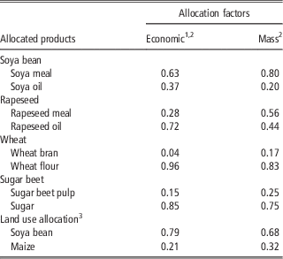
Table 1 shows the allocation factors used to partition GHG emissions and land use among feed co-products of a particular process. Economic allocation is our reference allocation method. Further discussion on allocation methods is presented in the sensitivity analysis.
Economic and mass allocation factors for co-products used in the two feeding scenarios for pig and dairy cow production in Sweden

1 Economic allocation is the default method, mass allocation is used in the sensitivity analysis.
2 Flysjö et al. (Reference Flysjo, Cederberg, Henriksson and Ledgard2012).
3 Land is allocated between soya bean and maize, which are double-cropped in the Centre West region of Brazil. Allocation is based on production data and supply prices (averaged for 2004–2009), taken from IBGE (2014).
Farm characteristics and data
The pig farms for the import and local scenarios are models of typical pig farms in south-eastern Sweden. Its dry climate and clayey soils favour cereal production for pigs. A farm in each scenario has 300 sows that produce 25 piglets/sow yearly with 1% mortality. The pigs are fattened to a live weight of 105 kg/pig (76.6 kg CW) over a 16.6-week period. The dairy farms for the import and local scenarios are models of typical dairy farms located in south-western Sweden. Humid weather conditions in this region favour forage crop production. The 100 cows on each farm produce 9000 kg ECM/cow annually. Data for feed resources on the pig and dairy farms were taken from a Swedish feed database (Flysjö et al., Reference Flysjö, Cederberg and Strid2008) that includes transportation distances for farm inputs, purchased feed and background assumptions applicable to feed resources. Background assumptions include emissions from fertiliser manufacturing, emissions from transport and data for purchased concentrate feed.
Pig production
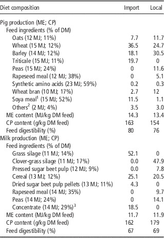
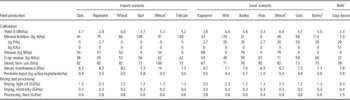
Table 2 shows the diets used for pigs in both scenarios. Feed intake is 3.64 kg dm feed/kg CW for the import and local scenarios (Cederberg and Flysjö, Reference Cederberg and Flysjö2004). The diet in the import scenario is composed of grains grown at the farm and imported soya meal. The crops are produced in a 5-year crop rotation of oats/rapeseed, winter wheat, barley, winter wheat, and triticale. Rapeseed is included in the first year to serve as an alternative in the otherwise cereal-based rotation. This rapeseed is sold to the market. The diet for the local scenario consists of grains, and the main protein part of rapeseed and peas, all grown at the farm. Rapeseed and peas are included in the crop rotation, resulting in a 7-year rotation: winter rape, winter wheat, barley, peas, winter wheat, oats and barley. Table 3 summarises the data for crop production taken from Flysjö et al. (Reference Flysjö, Cederberg and Strid2008) and Cederberg and Flysjö (Reference Cederberg and Flysjö2004). The effect of crop rotations on crop yields were based on field trials (Cederberg and Flysjö, Reference Cederberg and Flysjö2004; Engström, Reference Engström2010). Data on production of synthetic amino acids included in the pig diet were taken from Mosnier et al. (Reference Mosnier, van der Werf, Boissy and Dourmad2011).
Diet composition and characteristics of the two feeding scenarios (local and import) for pig (top panel) and dairy cow milk (bottom panel) production

ME=metabolisable energy; DM=dry matter.
1 Small amount of soya meal is used in the local scenario during the early fattening phase of the pigs.
2 Mainly straw and some minerals (mono-calcium phosphate).
3 Consists (by mass) of rapeseed meal (36%), soya meal (20%), sugar beet pulp (18%), palm kernel meal (7%) and small shares of other feed products.
Input parameters for the cultivation, drying and processing of crops used in two feeding scenarios for pig production in Sweden

DM=dry matter.
1 Both=both local and import feeding scenarios.
2 Last occurrence of a particular crop cultivated more than once in a crop rotation.
The pigs produced 690 and 870 kg fresh manure/pig per year, respectively, in the import and local scenarios. We calculated the amount of manure produced by assuming 87% volatile solids/kg dm manure and 8.8% dm content of manure (Dustan, Reference Dustan2002). The higher manure output of the local scenario is due to a large share of low digestible feeds (oats, rapeseed meal and wheat bran) in the diet (Table 2). N excreted in manure was 4.8 and 4.6 kg N/pig per year, respectively, for the import and local scenarios. N excreted is calculated as the difference between N in feed intake and N in carcass output. The higher N excretion of the import scenario is due to high N in feed intake from the large share of soya meal. Manure is stored for 10 months in well covered slurry tanks and spread on the farms (75% in spring, 25% in autumn) based on good agricultural practices and fertiliser guidelines (SBA, 2012).
Milk production
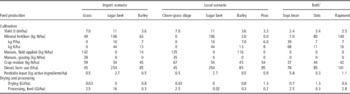
The diets were taken from Liljeholm et al. (Reference Liljeholm, Bertilsson and Strid2009) (Table 2). Feed intake was 0.72 and 0.69 kg dm feed/kg ECM for the import and local scenarios, respectively. The molasses is a by-product from sugar milling in southern Sweden. For the local scenario, the diet is designed to avoid feed from outside Sweden and includes grass/clover silage (25% clover). We assumed that rapeseed and peas are from neighbouring farms. In both scenarios, grains (barley and oats) are grown on one-third of the farm area. Any grain deficit is met by importing from neighbouring farms, where they are grown without input of manure. Table 4 summarises the data for crop production taken from Flysjö et al. (Reference Flysjö, Cederberg and Strid2008) and Liljeholm et al. (Reference Liljeholm, Bertilsson and Strid2009).
Input parameters for the cultivation, drying and processing of crops used in two feeding scenarios for dairy cow milk production in Sweden

DM=dry matter.
1 Both=both local and import feeding scenarios.
Manure output was estimated at 2100 and 1900 kg dry matter/cow per year, respectively, for the import and local scenarios, assuming 87% volatile solids/kg dm manure and 9.8% dm content of manure (Dustan, Reference Dustan2002). The cows graze for 2.5 months each year and excrete about 15% of the total manure on pasture. Manure is stored for 8 months as slurry with floating crust and spread on the farm (70% in late autumn, 30% in spring) at a rate of up to 170 kg N/ha. Mineral N fertilisers are used to fill the gap between the N input from manure and the N application rates recommended by SBA (2012). N excreted in manure is calculated as was done in pig production and amounts to 113 and 125 kg N/cow per year, respectively, for the import and local scenarios (Liljeholm et al., Reference Liljeholm, Bertilsson and Strid2009).
Life cycle GHG emission
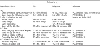
Table 5 shows the relevant emission factors and methods employed to estimate life cycle GHG emissions. CH4 emissions from enteric fermentation and manure management were calculated following relevant IPCC (2006) methods and tier I and tier II emission factors. Further discussion on the impact of different models for estimating enteric CH4 emission is presented in the sensitivity analysis. Emissions of NH3, N2O and leached nitrates were based on N excreted and applied on the field in the form of manure, synthetic fertilisers and crop residues. N in crop residues was taken from IPCC (2006). Emission factors for NH3 emissions were taken from Karlsson and Rodhe (Reference Karlsson and Rodhe2002). Other N emissions were based on IPCC (2006) emission factors at time of deposition, storage and application (Table 5). In the sensitivity analysis, we assess the impact of different emission factors on soil N2O emissions. Emissions from transporting farm inputs and feedstuff were calculated by multiplying transport distances and emission factors of the respective transport mode (Flysjö et al., Reference Flysjö, Cederberg and Strid2008). We assumed a distance of 10 km to neighbouring farms. GHG emissions from energy production were taken from the Ecoinvent (2007) database.
Emission factors quantifying greenhouse gas emissions from life cycle activities related to pig and dairy cow milk production in Sweden

GE=gross energy intake (import scenario=311 MJ/cow, local scenario=289 MJ/cow).
Ym=methane conversion factor (6.5%); MCF=methane conversion factor (Pigs=10%, Cows=8.5%); Bo=methane production capacity (Pigs=0.45, Cows=0.24); Vs=volatile solids excreted (calculated following IPCC (2006) method).
EF1=10% (spring application), 7% (autumn application).
EF2=forage crops 13.3%, grain crops 7%.
Land use
Land occupied was calculated as the product of crop yield and the feed required for pig or milk production while applying the allocation factors (Table 1). About 35% of soya bean land is cultivated with maize as a second crop in Centre West Brazil (IBGE, 2014). We handle this double cropping by allocating land use between soya bean and maize (Table 1).
LUC emissions
LUC is a key source of GHG emissions from agriculture (Gerber et al., Reference Gerber, Steinfeld, Henderson, Mottet, Opio, Dijkman, Falcucci and Tempio2013a); however, to date, there is no standardised approach in LCA to quantify LUC and translate it into GHG emissions. In this paper, we applied three alternative methods used to determine GHG emissions from LUC.
First, we estimated LUC emissions following the method of Gerber et al. (Reference Gerber, Steinfeld, Henderson, Mottet, Opio, Dijkman, Falcucci and Tempio2013a), which assumes that new soya bean crop area in Brazil is gained at the expense of forest land. LUC emission from soya bean expansion was calculated as the accumulated emissions for 1 year resulting from the total area deforested during the period 1991 to 2011 divided by the total soya bean production in 2011. We used FAOSTAT data to determine mean annual LUC rates for soya bean production, about 0.62 Mha/year, for the period 1991 to 2011. Forest conversion to annual cropland releases a mean of 37 t CO2-eq/ha during the 20 years (Gerber et al., Reference Gerber, Steinfeld, Henderson, Mottet, Opio, Dijkman, Falcucci and Tempio2013a). Based on these data, LUC emission was 6.2 kg CO2-eq/kg soya bean. We used 3.8 kg CO2-eq/kg of soya meal in this study after applying the allocation factors (including double-crop allocation) in Table 1.
With the second method, from BSI (2012), crop expansion in a given country is assumed to be at the expense of four land use types: forest, pasture, annual and perennial crops. Using FAOSTAT data, crop expansion 20 years before 2011 and the shares of LUC for the four land use types were determined. LUC emissions were calculated assuming that the new cropland is gained from other land types, either in equal proportion or in proportion to their relative rates of LUC change. We selected the higher of the two estimates as the LUC emission factor. Using the BSI (2012) calculation tool, three crops were attributed LUC emissions: 12.47 kg CO2-eq/m2 for soya bean in Brazil, 3.67 kg CO2-eq/m2 for wheat in Sweden and 5.31 kg CO2-eq/m2 for oil palm in Malaysia. The emission intensities were 2.8, 0.56 and 0.29 kg CO2-eq/kg, respectively, for soya meal, wheat and palm kernel meal after applying the allocation factors (Table 1) and crop yields (Tables 3 and 4).
The method of Audsley et al. (Reference Audsley, Brander, Chatterton, Murphy-Bokern, Webster and Williams2009) assumes that all demand for agricultural land contributes to LUC and should be allocated a share of worldwide LUC emissions. We assumed a LUC emission factor of 1.43 t CO2-eq/ha, as calculated in (Audsley et al., Reference Audsley, Brander, Chatterton, Murphy-Bokern, Webster and Williams2009), based on total LUC emission of 8.5 Gt CO2-eq, of which 58% is attributable to commercial agriculture (FAOSTAT, 2014), and 3475 Mha of land used globally for commercial agriculture. We allocated the emissions to the crops in our study based on their land area requirements per unit of production (Tables 3 and 4).
Results and discussion
GHG emissions
Following recommendations of Flysjo et al. (Reference Flysjo, Cederberg, Henriksson and Ledgard2012), we separate LUC GHG emissions and life cycle GHG emissions. The former is presented in the section on LUC. We categorised life cycle GHG emissions into three main GHG source categories: manure management, feed production and enteric fermentation.
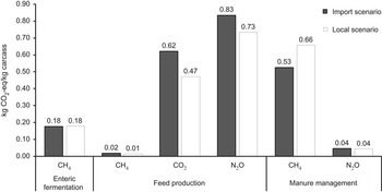
Total life cycle GHG emissions for pig production are 2.2 and 2.1 kg CO2-eq/kg CW for the import and local scenarios, respectively (Figure 1). The lower N2O emissions from feed production in the local scenario are closely linked to the inclusion of peas in the crop rotation. Peas fix N in their root nodules and subsequent crops in a crop rotation benefit from this activity as relatively less N input from external fertiliser is required (Nemecek et al., Reference Nemecek, von Richthofen, Dubois, Casta, Charles and Pahl2008). Less fertiliser use, in turn, decreases N2O emissions. The lower CO2 emission from feed production in the local scenario is explained by the diversity of the crop rotation practised. First, peas and rapeseed provide suitable home-grown protein in the diet so that a significant (ca. 62%) part of the emissions from transporting soya meal from Brazil to Sweden is avoided. In addition, the high frequency of break crops (peas and rapeseed) in the rotation benefits the local scenario in terms of lower diesel use on the farm (Table 3). Break crops do not carry over diseases in the stubble and have lower residual stubble loads than grains, which facilitates the adoption of conservation farming strategies such as reduced mechanical weeding (Kirkegaard et al., Reference Kirkegaard, Christen, Krupinsky and Layzell2008). Furthermore, less fertiliser use in the local scenario reduces CO2 emissions from fertiliser production. However, much of these benefits, in terms of reduced N2O under the local scenario are offset by the increased CH4 emissions associated with manure management. This is explained by relatively lower digestibility of several feed ingredients included in the local scenario. Relatively larger proportion of wheat bran, oats and rapeseed meal contributed to a lower digestibility of the diet under local scenario resulting in a higher manure output, which in turn resulted in higher CH4 emissions from manure management.
Life cycle greenhouse gas emissions of the two feeding scenarios for pig production, expressed as kg CO2-eq per kg pig carcass, and subdivided into three main source categories.

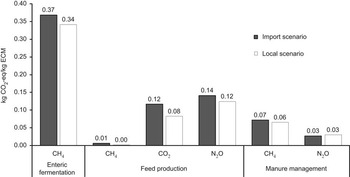
Total life cycle GHG emissions for milk production are 0.73 and 0.64 kg CO2-eq/kg CW for the import and local scenarios, respectively (Figure 2). When comparing the feed scenarios, the largest difference in emissions occurs during feed production. Under the local scenario, clover incorporated into forage production reduces the need for N and makes more manure available for the cereals produced; this, together with the N fertiliser avoided on the neighbouring pea farms, decreases N2O emissions and accounts for a significant (ca. 70%) part of the reduction in CO2 emissions from feed production. In our study, forage and grains are produced on the livestock farm, while other crops are imported from neighbouring farms. Based on our earlier observation from pig production, it may be argued that integrating the peas and rapeseed on the dairy farm could lead to further reductions in GHG emissions in milk production. The trade off, however, is that increasing crop diversity also limits economies of scale and may decrease farm net revenues and increase labour cost (Di Falco and Perrings, Reference Di Falco and Perrings2005). The clover-grass silage used in the local scenario decreases the roughage content of the diet, resulting in about 3% increase in feed digestibility (Table 2), which in turn reduces enteric CH4 emissions per unit of feed intake (McAllister et al., Reference McAllister, Okine, Mathison and Cheng1996).
Life cycle greenhouse gas emissions of the two feeding scenarios for dairy cow milk production, expressed as kg CO2-eq per kg energy corrected milk (ECM), and subdivided into three main source categories.

Life cycle GHG emissions are available in literature for some import and local feeding scenarios, although several methodological aspects make comparison difficult, such as different feedstuff compositions and system boundaries. Meul et al. (Reference Meul, Ginneberge, Van Middelaar, de Boer, Fremaut and Haesaert2012) estimated GHG emissions of import and local pig feed scenarios as 0.45 and 0.44 kg CO2-eq/kg feed, respectively. Our results, based on their system boundary, are 0.35 and 0.29 kg CO2-eq/kg feed, respectively, for the import and local scenarios. The 17% reduction in emission of our local scenario, compared with only 2% for Meul et al. (Reference Meul, Ginneberge, Van Middelaar, de Boer, Fremaut and Haesaert2012), is closely linked to the benefits of diverse crop rotations included in our local scenario. For milk production, Lehuger et al. (Reference Lehuger, Gabrielle and Gagnaire2009) obtained 0.39 and 0.47 kg CO2-eq/kg feed, respectively, for import and local feed scenarios; compared with 0.36 and 0.30 kg CO2-eq/kg feed, respectively, obtained in this study. The increase in diversity we observe from multiple crops in our local scenario may explain the contradiction in results. But it is difficult to compare our results with Lehuger et al. (Reference Lehuger, Gabrielle and Gagnaire2009) since they used the mass allocation method. Lehuger et al. (Reference Lehuger, Gabrielle and Gagnaire2009) and Meul et al. (Reference Meul, Ginneberge, Van Middelaar, de Boer, Fremaut and Haesaert2012) limit their system boundaries to capture only emissions from feed production. However, reductions in emissions in the field may not necessarily correspond to emissions in the stable (Gerber et al., Reference Gerber, Hristov, Henderson, Makkar, Oh, Lee, Meinen, Montes, Ott, Firkins, Rotz, Dell, Adesogan, Yang, Tricarico, Kebreab, Waghorn, Dijkstra and Oosting2013b). In our study, focusing on only feed production for pigs would ignore the higher manure emissions of the local scenario and exaggerate the avoided GHG emissions of local feed production (Figure 1).
Land use
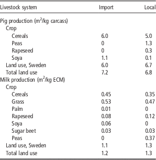
Total yearly land use for pig production is 7.2 and 6.8 m2/kg CW, respectively, for the import and local scenarios (Table 6). The lower land use for the local scenario is due to the increase in wheat yields achieved from the diverse crop rotation (Kirkegaard et al., Reference Kirkegaard, Christen, Krupinsky and Layzell2008). However, the difference in land use between the two scenarios is not as large as one would expect due to the substantial increase (ca. 24% of total) in land use for domestic protein crops, especially peas in the local scenario (Table 6). Generally, land use is determined by the crop yield, allocation factors of co-products, and in the case of soya bean, allocation of land due to double cropping of maize and soya beans (Table 1). Peas have higher mean crop yields than rapeseed in the region studied, but the low land requirement for rapeseed meal is related to the fact that when the impacts of rapeseed cultivation is shared between the two co-products (meal and oil), rapeseed meal benefits because of its low economic value (Table 1).
Land use on annual basis under two feeding scenarios for pig production (top panel) and dairy cow milk production (bottom panel) in Sweden

ECM=energy corrected milk.
For milk production, total yearly land use is 1.2 and 1.3 m2/kg ECM, respectively, for the import and local scenarios (Table 6). A significant part of the land area in both scenarios is used for forage crop production. Despite the decrease in forage and grain areas, land use for the local scenario increases due to additional land required for producing peas.
When Eriksson et al. (Reference Eriksson, Elmquist, Stern and Nybrant2005) compared import and local feed scenarios for Swedish pigs, the local scenarios required more land than the import scenario. The conflict between their results and ours is because we consider the yield effect of crop rotations.
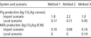
GHG emission from LUC
In this study, localising protein feed production increased the land required in Sweden for producing pig and dairy diets (Table 6). Increased demand for land in Sweden would be at the expense of other land use in Sweden (direct LUC) and elsewhere (indirect LUC). Thus, it is important to account for emissions from the LUC. Table 7 shows LUC emissions for the feed scenarios, calculated with three alternative methods. For pig production, the ranking of LUC emissions of the feed scenarios is the same for the three methods (and similar to the ranking for the life cycle GHG emissions). For milk production, however, the method from Audsley et al. (Reference Audsley, Brander, Chatterton, Murphy-Bokern, Webster and Williams2009) assigns more emissions to the local scenario because of its higher land use.
Greenhouse gas emissions from land use change estimated by three alternative methods for pig and dairy cow milk production

Method 1=calculation based on Gerber et al. (2013a); Method 2=calculation based on BSI (2012); Method 3=calculation based on Audsley et al. (Reference Audsley, Brander, Chatterton, Murphy-Bokern, Webster and Williams2009).
ECM=energy corrected milk.
The accounting methods show that both import and local scenarios contribute to LUC emissions globally. How accurately the accounting methods capture the potential LUC from both feeding scenarios can be a matter for further discussion. The method of Gerber et al. (Reference Gerber, Steinfeld, Henderson, Mottet, Opio, Dijkman, Falcucci and Tempio2013a) focuses only on the expansion of soya beans in Brazil; thus, LUC from protein crop expansion in Sweden is ignored, and feed scenarios with soya bean products are penalised. The method of BSI (2012) captures the LUC emissions from all crops in a given country. However, it is not possible with this method to analyse how protein feed production in Sweden influences LUC outside Sweden. The method of Audsley et al. (Reference Audsley, Brander, Chatterton, Murphy-Bokern, Webster and Williams2009) captures total LUC (direct and indirect) but it does not distinguish between feeds with similar land requirements. An implication of using the Audsley et al. (Reference Audsley, Brander, Chatterton, Murphy-Bokern, Webster and Williams2009) method is that rapeseed on established cropland in Sweden would be assigned the same LUC emissions as soya bean on recently deforested land in Brazil, given that they have the same yields.
In reality, LUC are far more complex than presented above, and establishing a link between a specific land occupation and an observed LUC can be difficult. Demand for land is influenced by feed demand but also subject to competition from food and bioenergy demands and trade between countries, all of which influence LUC (Hertel et al., Reference Hertel, Golub, Jones, O’Hare, Plevin and Kammen2010). Recent efforts to account for such complex interactions have been in the bioenergy sector, where mostly economic models of bioenergy markets are used to simulate competition for land in response to market demands. Similar models comprising relevant agricultural markets can improve accounting of LUC from agriculture if challenges of data availability are resolved (Cederberg et al., Reference Cederberg, Henriksson and Berglund2013).
Sensitivity analysis
The results of this study depend on our assumptions about the farm systems. Due to differences in agronomic and climatic factors across regions, our assumptions may be applicable only in the studied regions of Sweden and Brazil. Several aspects of our study were also analysed in a three-part sensitivity analysis to check their influence on the results.
Allocation factors for co-products
We used economic allocation as the main method in our study to reflect the economic driving force behind agriculture and feed production. In the sensitivity analysis, we applied mass-based allocation. Allocation due to double cropping was also contrasted with a scenario of no double cropping. Using mass allocation, there was no difference in GHG emissions for the feeding scenarios in pig production, resulting in about 2.3 kg CO2-eq/kg CW. This is because mass allocation assigns more emissions to rapeseed meal and wheat bran (Table 1), which are important ingredients in the local ration. For similar reasons, the local pig scenario required 4% more land than the import scenario. However, the local scenario requires about 9% less land when we exclude the allocation for double cropping. For milk production, the local scenario decreased GHG emissions by 12% compared with the import scenario after applying mass allocation. Similar reduction was observed with the economic allocation method. Land use was relatively unchanged, that is, higher land use for the local scenario than the import scenario.
N2O emissions
Direct N2O emissions are often estimated using the IPCC (2006) emission factor of 1%, but actual emissions for a given input may vary substantially with soil type, climate conditions and source of N input. In the sensitivity analysis, we applied differentiated emission factors from Lesschen et al. (Reference Lesschen, Velthof, de Vries and Kros2011): 0.1%, 0.6%, 1.2%, and 2.5% for crop residues of cereals, rapeseed, peas and soya bean, respectively; 0.4% for manure; and 0.2% and 1% from N fertiliser in Sweden and Brazil, respectively. The differentiated emission factors reduced total GHG emissions by 16% in both pig scenarios, but the ranking of the scenarios remained unchanged. Differences in N2O emission factors are important, but of little relevance when comparing GHG emissions from the two scenarios. This is because a large share of feedstuff was cultivated on farms in Sweden with similar systems and climatic conditions.
Enteric CH4 emissions
The composition of dairy cow diets influenced enteric CH4 emissions of the animals. However, the emissions estimated depend on the model used. As a base case, we used the IPCC (2006) model to estimate enteric CH4 emissions as 132 and 123 kg CH4/cow, respectively, for the import and local scenarios. Liljeholm et al. (Reference Liljeholm, Bertilsson and Strid2009) assessed seven other models for estimating enteric CH4 emissions, which we used in a sensitivity analysis. When applied to our study, outputs from the seven models ranged from 108 to 153 kg CH4/cow for the import scenario and 106 to 140 kgCH4/cow for the local scenario. The ranking of dairy scenarios in our study according to their total GHG emissions remain unchanged for all model estimates. Thus, our choice of CH4 emission model does not change the results.
Conclusions
We assessed impacts of local protein feed production on GHG emissions and land use for pig and dairy cow production in Sweden, compared with importing protein feed from outside Sweden. We find that local protein feed production presents an opportunity to reduce GHG emissions by about 4.5% and 12%, respectively, for pigs and dairy cows fed with locally produced feedstuff. Decreased emissions come at a cost of increased land occupation in Sweden for feed production. Additional land in Sweden for feed production was 11% for pigs and 25% for dairy cows.
Local production of protein feed decreases inputs needed for production and improves some ecological processes of the farming system, which largely explain the decreases in emissions. For pig production, local production of protein feeds improves the diversity of a cereal-based crop rotations, leading to decreased use of mineral fertiliser and fossil fuels, and higher yields of grain crops. However, there is no corresponding decrease in GHG emissions from rearing the pigs due to lower digestibility of the feed ration when using the locally produced protein feedstuff. This latter conclusion highlights the importance of focusing on both feed production and animal production when assessing feed substitutions. For milk production, legumes reduce mineral fertiliser input, and the grass–legume mixture increases the digestibility of the animal feed, which explain the decreases in emissions.
The performance of local protein feed production depends on characteristics of the farm systems compared, as well as on the choice of methods, such as impact allocation method and LUC accounting method. In the case of pig production, the benefit of local production is relatively small and sensitive to the impact allocation method applied. Local feed production induces LUC in Sweden and elsewhere. However, we find that the LUC accounting methods available may not adequately account for the potential LUC and the emissions associated with local protein feed production.
Acknowledgement
The authors gratefully acknowledge financial support by the Swedish Farmers’ Foundation for Agricultural Research.