1. Introduction
Baroclinic instability is recognized to be one of the dominant energetic processes in the large-scale atmospheres of terrestrial planets, such as the Earth and Mars (Pierrehumbert & Swanson Reference Pierrehumbert and Swanson1995), and in the oceans (Orlanski & Cox Reference Orlanski and Cox1973). Its fully developed form as sloping convection is strongly nonlinear and has a major role in the transport of heat and momentum in the atmospheric and oceanic motions. Its time-dependent behaviour also exerts a dominant influence on the intrinsic predictability of the atmospheric circulation and the degree of chaotic variability in its large-scale meteorology (Pierrehumbert & Swanson Reference Pierrehumbert and Swanson1995; Read et al. Reference Read, Collins, Früh, Lewis and Lovegrove1998; Read Reference Read2001). Inertia–gravity waves (IGWs) are ubiquitous in the atmosphere and the oceans and are known to play a fundamental role in a wide variety of processes. The contributions mainly concern the transport of a significant amount of energy and momentum, the initiation and organization of convection, the induction and modulation of turbulence, as well as the modification of the mean circulation and thermal structure of atmospheric and oceanic motions (Fritts & Alexander Reference Fritts and Alexander2003). We refer to the reference books by LeBlond & Mysak (Reference LeBlond and Mysak1978), Lighthill (Reference Lighthill1978), Gill (Reference Gill1982) and Nappo (Reference Nappo2003) for the fundamental wave properties of IGWs. These waves, exhibiting rotational and gravitational oscillations, are supported by rotating, stably stratified flows, where buoyancy and Coriolis forces act as restoring forces. Observations and simulations have revealed their spontaneous occurrence during the development of baroclinic instability. In spite of intensive research activities carried out over recent decades, the generation mechanism and the propagation of IGWs, as well as their interaction with large-scale structures, remain poorly understood. A better understanding of these phenomena is therefore mandatory for the improvement of the IGW parameterization schemes required to upgrade numerical global weather predictions. On the other hand, Orlanski & Cox (Reference Orlanski and Cox1973) reported the close analogy between the dynamics of the ocean and the atmosphere, and concluded that the same baroclinic mechanism may operate in both environments.
Since the pioneering work of Hide (Reference Hide1958), the differentially heated, rotating cylindrical annulus has been an archetypal means of studying the properties of fully developed baroclinic instability in the laboratory. The system is well-known to exhibit a rich variety of different flow regimes, depending upon the imposed conditions (primarily the temperature contrast
 ${\rm\Delta}T$
and rotation rate
 ${\it\Omega}$
in a fixed geometry for a given fluid), ranging from steady, axisymmetric circulations through highly symmetric, regular wave flows to fully developed geostrophic turbulence (Hide Reference Hide1958; Fowlis & Hide Reference Fowlis and Hide1965).
The main sources proposed for gravity wave generation are mountain waves forced by flow over topography, convection, unstable shear zones and jets/fronts, although other sources may also be significant (see the review articles by Lindzen Reference Lindzen, Holton and Matsuno1984, Fritts & Alexander Reference Fritts and Alexander2003, Vanneste Reference Vanneste2013 and Plougonven & Zhang Reference Plougonven and Zhang2014). In the ocean the internal gravity waves can be generated by fluctuations of atmospheric pressure, by buoyancy flow at the ocean surface and by wind. Nonlinear mechanisms have been studied during the generation of nonlinear resonant waves by the coupling of surface waves (Miropol’sky Reference Miropol’sky and Shishkina2001).
Gravity waves generated by mountains have been extensively studied in the past four decades using observational, theoretical and numerical methods, and the responses to the topography have been reasonably well understood (Belcher & Hunt Reference Belcher and Hunt1998; Fritts & Alexander Reference Fritts and Alexander2003). Several mechanisms have been proposed for the generation of gravity waves associated with convection, including the effect of obstacles, the mechanical oscillator effect (excitation by vertical oscillation of updrafts and downdrafts, convective plumes (Ansong & Sutherland Reference Ansong and Sutherland2010)) and pure thermal forcing (Fritts & Alexander Reference Fritts and Alexander2003). The generation and propagation of IGWs in shear flows have also been the subject of theoretical studies using idealized models. In an earlier paper, Lindzen (Reference Lindzen1974) showed that a Helmholtz velocity profile in an infinite fluid with constant stable stratification throughout would sustain not only Kelvin–Helmholtz instabilities but also neutral internal gravity waves radiating energy away from the interface. Although Lindzen (Reference Lindzen1974) only investigated solutions with zero real phase speed, neutral radiating solutions with non-zero phase speed also exist which are continuations of Kelvin–Helmholtz instabilities at low wavenumbers (Lindzen & Rosenthal Reference Lindzen and Rosenthal1976). The linear stability of an unbounded stratified shear layer has provided results on resonant over-reflection and on the propagating wave instabilities that can develop when the shear layer becomes unstable. Energy analysis indicates that the physical mechanisms driving trapped modes and propagating modes are very similar and the radiating wave instability can be viewed as the linear excitation of propagating waves by a Kelvin–Helmholtz unstable mode existing at the shear layer (Lott, Kelder & Teitelbaum Reference Lott, Kelder and Teitelbaum1992).
Other sources of internal gravity waves are wave excitation by geostrophic adjustment of unbalanced flows in the vicinity of jet streams and frontal systems, body forces accompanying localized wave dissipation, wave–wave interactions and spontaneous emission. Gravity wave excitation by geostrophic adjustment occurs when a flow is forced away from a state governed by geostrophic balance, where the pressure gradients are nearly balanced by Coriolis force in the horizontal plane and by buoyancy gradients in the vertical (hydrostatic balance). Flows with a small Rossby number, corresponding to strong rotation, are well-balanced and have time scale separation between slow-balanced motion and fast IGWs (see the review article by Vanneste Reference Vanneste2013). Recent comprehensive reviews on the waves emitted near jets and fronts in the atmosphere have been made by Vanneste (Reference Vanneste2013) and Plougonven & Zhang (Reference Plougonven and Zhang2014). In particular, Plougonven & Zhang (Reference Plougonven and Zhang2014) brought further clarification on the distinction between the different mechanisms involved, namely geostrophic adjustment, spontaneous adjustment emission where waves originate from initially balanced flow, including Lighthill radiation, unbalanced instabilities and transient generation (Lighthill Reference Lighthill1978; Ford Reference Ford1994), and reported on the further evolution of internal waves. (See also Staquet & Sommeria Reference Staquet and Sommeria2002 for a comprehensive review of the mechanisms of steepening and breaking of internal gravity waves in a continuous density stratification, as well as of the parameterization of their effects in turbulence models.)
Many observational studies on gravity waves have been conducted using time series of velocity profiles, that provide evidence and characteristics of the waves such as group velocity and the energy source (Leaman & Sanford Reference Leaman and Sanford1975; Thompson Reference Thompson1978; Thomas, Worthingthon & McDonald Reference Thomas, Worthingthon and McDonald1999; Tateno & Sato Reference Tateno and Sato2008). Tateno & Sato (Reference Tateno and Sato2008) studied the source of IGW packets in the middle stratosphere using a ray-tracing method and the results indicated that IGWs packets were generated in the vicinity of the unbalanced westerly jet due to spontaneous adjustment processes.
Different theoretical models have been used to investigate numerically the emission of IGWs in simulated flows, such as jets within a vortex dipole, an evolving baroclinic flow, or a stratified shear flow. Some studies of gravity wave excitation have been focused on the generation of IGWs by geostrophic adjustment of the tropospheric jet stream as it is distorted by a developing baroclinic wave (O’Sullivan & Dunkerton Reference O’Sullivan and Dunkerton1995; Zhang Reference Zhang2004). Zhang (Reference Zhang2004) proposed a generalization of the geostrophic adjustment hypothesis, balance adjustment, as the likely mechanism in generating these mesoscale gravity waves in the unbalanced upper-tropospheric jet–front systems. Spontaneous generation by balanced flows has been obtained from simulations of the propagation of IGWs from vortex dipoles. For instance, an initially balanced flow consisting of an unstable baroclinic jet was observed to break up into a street of cyclonic and anticyclonic vortices (Viúdez & Dritschel Reference Viúdez and Dritschel2006; Pàllas-Sanz & Viúdez Reference Pàllas-Sanz and Viúdez2008). The instability of a three-dimensional (baroclinic) jet was also reported using a triply periodic non-hydrostatic numerical model (Dritschel & Viúdez Reference Dritschel and Viúdez2003; Viúdez & Dritschel Reference Viúdez and Dritschel2006). In this model, a balanced flow spontaneously emits bursts of IGWs from a source located at the largest curvature side of the emerging highly ageostrophic anticyclonic vortex in a region of large advection. They propagate both outward – away from the vortex – as a wave packet and inward, where they appear trapped. The behaviour of a small-amplitude IGW packet propagating in a baroclinic shear flow has been investigated using WKB theory and direct numerical simulations (DNS) by Edwards & Staquet (Reference Edwards and Staquet2005).
The generation of internal waves in the laboratory has been studied in an annular cavity by Williams, Read & Haine (Reference Williams, Read and Haine2003) and Williams, Haine & Read (Reference Williams, Haine and Read2005) within a two-layer fluid. Using the ray approach proposed by Ford (Reference Ford1994) to locate sources of IGWs, Williams et al. (Reference Williams, Read and Haine2003) investigated the possibility of the generation of IGWs from a Kelvin–Helmholtz shear instability by correlating regions of laboratory IGW production and regions where the Richardson number is subcritical. They found that spontaneous emission, rather than a Kelvin–Helmholtz shear instability, is responsible for the production of the observed laboratory IGWs.
Jacoby et al. (Reference Jacoby, Read, Williams and Young2011) carried out DNS in a differentially heated, rotating annulus, the baroclinic cavity, filled with a high-Prandtl-number fluid (
 $Pr=24$
). When baroclinic instability sets in, some small-scale wave packets characterized by a short period are observed attached to the ridges of the baroclinic waves, near the inner cylindrical cold wall, and identified as IGWs. A boundary layer flow develops with the axial velocity directed downward along this vertical wall, and the authors explored the instability of this layer as a source of the IGWs. Based on linear theory results in buoyancy-driven systems without rotation (Gill & Davey Reference Gill and Davey1969) these authors concluded that the instability of the boundary layer along the cold inner cylinder might be responsible for the generation of the numerically obtained IGWs. Recently, Borchert, Achatz & Fruman (Reference Borchert, Achatz and Fruman2014) reported from DNS the occurrence of additional IGWs with respect to those found by Jacoby et al. (Reference Jacoby, Read, Williams and Young2011) when using water (
 $Pr=7$
) in a baroclinic configuration characterized by a Brunt–Väisälä frequency larger than the inertial frequency, unlike in the situation studied by Jacoby et al. (Reference Jacoby, Read, Williams and Young2011). This was to mimic the behaviour commonly observed in the actual atmosphere, by imposing a larger temperature difference associated with a smaller rotation rate but requiring radial extent larger than the height. They mentioned that the source of IGWs was spontaneous emission from imbalances of the large-scale baroclinic wave, similarly to the findings of O’Sullivan & Dunkerton (Reference O’Sullivan and Dunkerton1995) and Plougonven & Snyder (Reference Plougonven and Snyder2007) during their simulations of idealized baroclinic life cycles. Jacoby et al. (Reference Jacoby, Read, Williams and Young2011) used a cavity covered by a rigid lid at the top, while in the case of Borchert et al. (Reference Borchert, Achatz and Fruman2014), an open upper free surface was considered.
In the present work some characteristics of the IGWs within a baroclinic cavity are determined from the analysis of the velocity and temperature fields provided by DNS. The working fluid corresponds to a liquid defined by
 $Pr=16$
following the experimental investigations carried out by Wordsworth (Reference Wordsworth2009). A three-term decomposition is introduced to isolate the fluctuation field from the large-scale baroclinic waves and the mean flow. The aim is to apply the results of the linear theory to better understand the wave propagation and to analyse the source.
2. Mathematical model and solution method for the direct numerical simulation
2.1. Governing equations
The physical model, the so-called ‘baroclinic cavity’, consists of an annular domain of inner radius
 $a$
, outer radius
 $b$
and height
 $d$
, uniformly rotating around its vertical axis of symmetry with an angular velocity
 ${\it\Omega}$
. The cavity is filled with a liquid defined by a Prandtl number
 $Pr$
and is subjected to a temperature difference
 ${\rm\Delta}T$
between the inner, cold cylinder at temperature
 $T_{a}$
, and outer, hot cylinder at temperature
 $T_{b}$
, closed by horizontal insulating rigid endplates.
In the meridional plane, the dimensional space variables
 $(r^{\ast },z^{\ast })$
 $\in$
 $[a,b]\times [0,d]$
have been normalized into the square
 $[-1,1]\times [-1,1]$
, a prerequisite for the use of Chebyshev polynomials (* denotes dimensional variables):
 $$\begin{eqnarray}\displaystyle r=\frac{2r^{\ast }}{(b-a)}-\frac{(b+a)}{(b-a)},\quad z=\frac{2z^{\ast }}{d}-1. & & \displaystyle\end{eqnarray}$$
However, in the graphical representations, the dimensionless axial coordinate was in the range
 $z\in [0,A\equiv d/(b-a)]$
to enhance vertical variations.
The fluid is assumed to satisfy the Boussinesq approximation (see Lopez, Marques & Avila Reference Lopez, Marques and Avila2013), with constant properties except for the density when applied to the centrifugal and gravitational accelerations where
 ${\it\rho}={\it\rho}_{0}(1-{\it\alpha}(T-T_{0}))$
, where
 ${\it\alpha}$
is the coefficient of thermal expansion and
 $T_{0}$
is a reference temperature
 $T_{0}=(T_{b}+T_{a})/2$
. The reference scales are the velocity
 $U^{\ast }=g{\it\alpha}{\rm\Delta}T/2{\it\Omega}$
and the time
 $t^{\ast }=(2{\it\Omega})^{-1}$
, and the non-dimensional normalized temperature is
 $2(T^{\ast }-T_{0})/{\rm\Delta}T$
, where
 ${\rm\Delta}T=(T_{b}-T_{a})$
(see Randriamampianina et al.
Reference Randriamampianina, Früh, Maubert and Read2006; Randriamampianina & Crespo del Arco Reference Randriamampianina, Crespo del Arco, von Larcher and Williams2014).
In the present case, a water–glycerol mixture defined by a Prandtl number
 $Pr=16$
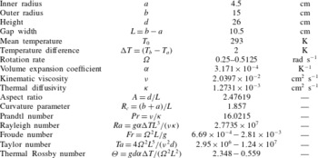
has been considered, following experimental investigations carried out by Wordsworth (Reference Wordsworth2009). The details of the system, the fluid properties and the governing parameters are summarized in table 1. The configuration consists of an annular domain of inner radius
 $a=4.5~\text{cm}$
, outer radius
 $b=15~\text{cm}$
and height
 $d=26~\text{cm}$
(Wordsworth Reference Wordsworth2009). The cavity is subjected to a temperature difference
 ${\rm\Delta}T=2~\text{K}$
between the inner, cold, and outer, hot, cylinders closed by horizontal insulating rigid endplates. The simulations concern three values of the rotation rate, covering different flow regimes of baroclinic waves:
 ${\it\Omega}=0.25,0.35$
and
 $0.5125~\text{rad}~\text{s}^{-1}$
.
Summary of the dimensions of the system, the fluid properties and units, and the governing parameters for the liquid-filled cavity.

Depending on the type of solution sought, axisymmetric or non-axisymmetric, two different approaches are considered independently for the governing equations of the flow dynamics. In the first case, a vorticity–streamfunction with azimuthal velocity formulation is introduced. Not only does it reduce the number of equations to solve, in comparison with the primitive variables velocity–pressure formulation, but it also ensures a divergence-free velocity field irrespective of the mesh used. An influence matrix technique is implemented to treat the lack of boundary conditions for the vorticity coupled with the streamfunction (Chaouche, Randriamampianina & Bontoux Reference Chaouche, Randriamampianina and Bontoux1990; Randriamampianina, Schiestel & Wilson Reference Randriamampianina, Schiestel and Wilson2001, Reference Randriamampianina, Schiestel and Wilson2004). For the three-dimensional solution, the primitive variables are directly solved. We recall below the details of the governing equations and the numerical method used.
In a reference frame rotating with the cavity, the resulting dimensionless system is written (Randriamampianina et al. Reference Randriamampianina, Früh, Maubert and Read2006; Randriamampianina & Crespo del Arco Reference Randriamampianina, Crespo del Arco, von Larcher and Williams2014)
 $$\begin{eqnarray}\displaystyle & \displaystyle \frac{\partial \boldsymbol{V}}{\partial t}+\frac{2Ra}{A^{2}PrTa}N(\boldsymbol{V})+\boldsymbol{e}_{z}\times \boldsymbol{V}=-\boldsymbol{{\rm\nabla}}{\it\Pi}+\frac{4}{A^{3/2}Ta^{1/2}}{\rm\nabla}^{2}\boldsymbol{V}+\boldsymbol{F}, & \displaystyle\end{eqnarray}$$
 $$\begin{eqnarray}\displaystyle & \displaystyle \boldsymbol{{\rm\nabla}}\boldsymbol{\cdot }\boldsymbol{V}=0, & \displaystyle\end{eqnarray}$$
 $$\begin{eqnarray}\displaystyle & \displaystyle \frac{\partial T}{\partial t}+\frac{2Ra}{A^{2}PrTa}\boldsymbol{{\rm\nabla}}\boldsymbol{\cdot }(\boldsymbol{V}T)=\frac{4}{A^{3/2}PrTa^{1/2}}{\rm\nabla}^{2}T, & \displaystyle\end{eqnarray}$$
 $$\begin{eqnarray}\displaystyle & \displaystyle N(\boldsymbol{V})={\textstyle \frac{1}{2}}\boldsymbol{V}\boldsymbol{\cdot }\boldsymbol{{\rm\nabla}}\boldsymbol{V}+{\textstyle \frac{1}{2}}\boldsymbol{{\rm\nabla}}\boldsymbol{\cdot }(\boldsymbol{V}\boldsymbol{V}), & \displaystyle\end{eqnarray}$$
 $$\begin{eqnarray}\displaystyle & \displaystyle {\it\Pi}=\frac{p+{\it\rho}_{0}gz-\frac{1}{2}{\it\rho}_{0}{\it\Omega}^{2}r^{2}}{{\it\rho}_{0}g{\it\alpha}(T_{b}-T_{a})d/2}, & \displaystyle\end{eqnarray}$$
 $$\begin{eqnarray}\displaystyle & \displaystyle \boldsymbol{F}=\frac{1}{2}T\boldsymbol{e}_{z}-\frac{Fr}{4A}(r+R_{c})T\boldsymbol{e}_{r}, & \displaystyle\end{eqnarray}$$
 $\boldsymbol{e}_{r}$
and
 $\boldsymbol{e}_{z}$
are the unit vectors in the radial and axial directions respectively, and
 $N(\boldsymbol{V})$
represents the nonlinear advection terms. The external force
 $\boldsymbol{F}$
results from the application of the Boussinesq approximation to the gravity and the centrifugal acceleration, corresponding to the perturbation of the density (Randriamampianina et al.
Reference Randriamampianina, Früh, Maubert and Read2006; Lopez et al.
Reference Lopez, Marques and Avila2013). The parameters governing the flow and the heat transfer are the aspect ratio
 $A$
, the curvature parameter
 $R_{c}$
, the Prandtl number
 $Pr$
, the Rayleigh number
 $Ra$
, the Froude number
 $Fr$
, and the Taylor number
 $Ta$
(see the definitions in table 1). For a given fluid within a fixed geometry, the Taylor number is one of the two main control parameters traditionally used to analyse this system, following Fowlis & Hide (Reference Fowlis and Hide1965) and Hide & Mason (Reference Hide and Mason1975). The second parameter is the thermal Rossby number,
 $$\begin{eqnarray}{\it\Theta}=\frac{gd{\it\alpha}(T_{b}-T_{a})}{{\it\Omega}^{2}L^{2}}\equiv \frac{4Ra}{PrTa},\end{eqnarray}$$
introduced by Hide (Reference Hide1958) as a stability parameter, which gives a measure of the buoyancy strength compared to the Coriolis term and appears explicitly as coefficient of the convection terms in (2.2) and (2.4).
The ‘skew-symmetric’ form proposed by Zang (Reference Zang1990) was chosen for the nonlinear advection terms
 $N(\boldsymbol{V})$
in the momentum equations to ensure the conservation of kinetic energy, a necessary condition for a simulation to be numerically stable in time.
2.2. Boundary conditions
The boundary conditions are no-slip velocity conditions at all rigid surfaces,
 $$\begin{eqnarray}\displaystyle \boldsymbol{V}=\mathbf{0}\quad \text{at }r=\pm 1\text{ and at }z=\pm 1, & & \displaystyle\end{eqnarray}$$
thermal insulation at horizontal rigid surfaces,
 $$\begin{eqnarray}\displaystyle \frac{\partial T}{\partial z}=0\quad \text{at }z=\pm 1 & & \displaystyle\end{eqnarray}$$
and constant temperature conditions at the vertical sidewalls,
 $$\begin{eqnarray}\displaystyle T=\pm 1\quad \text{at }r=\pm 1. & & \displaystyle\end{eqnarray}$$
2.3. Temporal scheme
The time integration used is second-order accurate and is based on a combination of Adams–Bashforth and backward differentiation formula schemes, chosen for its good stability properties (Vanel, Peyret & Bontoux Reference Vanel, Peyret, Bontoux, Morton and Baines1986). The resulting AB/BDF scheme is semi-implicit, and for the transport equation of the velocity components in (2.2) is written
 $$\begin{eqnarray}\displaystyle \frac{3f^{l+1}-4f^{l}+f^{l-1}}{2{\it\delta}t}+2\mathscr{N}(f^{l})-\mathscr{N}(\,f^{l-1})=-\boldsymbol{{\rm\nabla}}{\it\Pi}^{l+1}+\frac{4}{A^{3/2}Ta^{1/2}}{\rm\nabla}^{2}f^{l+1}+F_{i}^{l+1},\hspace{20.00003pt} & & \displaystyle\end{eqnarray}$$
where
 $\mathscr{N}(f)$
is a ‘global’ term which includes the nonlinear advection terms with the Coriolis term and the cross-terms in the diffusion part in the
 $(r,{\it\theta})$
plane resulting from the use of cylindrical coordinates in (2.2). This ‘global’ term
 $\mathscr{N}(f)$
is discretized in time with an explicit second-order Adams–Bashforth scheme (2.12), in order to maintain an overall second-order time accuracy.
 $F_{i}$
corresponds to the component of the forcing term
 $\boldsymbol{F}$
,
 ${\it\delta}t$
is the time step and the superscript
 $l$
refers to time level. An equivalent discretization applies for the transport equation of the temperature (2.4). For the initial step, we have taken
 $f^{-1}=f^{0}$
. At each time step, the problem then reduces to the solution of successive Helmholtz and Poisson equations.
2.4. Numerical approach
A pseudospectral collocation–Chebyshev method is implemented in the meridional plane
 $(r,z)$
, in association with a Galerkin Fourier approximation in azimuth
 ${\it\theta}$
for the three-dimensional flow regimes, to solve the primitive variables formulation described above. Each dependent variable is expanded in the approximation space
 $\mathscr{P}_{NM}$
, composed of Chebyshev polynomials of degrees less than or equal to
 $N$
and
 $M$
in the
 $r$
- and
 $z$
- directions respectively, while Fourier series are introduced in the azimuthal direction with
 $K$
modes.
For each dependent variable
 $f$
(
 $f\equiv V_{r},V_{{\it\theta}},V_{z},T,p$
) it is written as
 $$\begin{eqnarray}f_{NMK}(r,{\it\theta},z,t)=\mathop{\sum }_{n=0}^{N}\,\mathop{\sum }_{m=0}^{M}\,\mathop{\sum }_{k=-K/2}^{K/2-1}\,\hat{f}_{nmk}(t)T_{n}(r)T_{m}(z)\exp (\text{i}k{\it\theta}),\end{eqnarray}$$
where
 $T_{n}$
and
 $T_{m}$
are Chebyshev polynomials of degrees
 $n$
and
 $m$
.
This approximation is applied at collocation points, where the differential equations are assumed to be satisfied exactly (Gottlieb & Orszag Reference Gottlieb and Orszag1977; Canuto et al.
Reference Canuto, Hussaini, Quarteroni and Zang1987). We have chosen the Chebyshev–Gauss–Lobatto distribution defined by a high concentration of points towards the boundaries, well-suited to handle the thin dynamical and thermal boundary layers expected to develop at high values of the Taylor and Rayleigh numbers, which scale as
 $Ta^{-1/4}$
(Ekman layer, along horizontal walls) or
 $Ta^{-1/6}$
(Stewartson layer, along vertical cylinders) and
 $Ra^{-1/4}$
respectively:
 $$\begin{eqnarray}\displaystyle & \displaystyle r_{i}=\cos \left(\frac{i{\rm\pi}}{N}\right)\quad \text{for }i\in [0,N], & \displaystyle\end{eqnarray}$$
 $$\begin{eqnarray}\displaystyle & \displaystyle z_{j}=\cos \left(\frac{j{\rm\pi}}{M}\right)\quad \text{for }j\in [0,M], & \displaystyle\end{eqnarray}$$
 $$\begin{eqnarray}\displaystyle {\it\theta}_{k}=\frac{2k{\rm\pi}}{K}\quad \text{for }k\in [0,K\ $Pr=13.07$
) with respect to the detailed results reported by Hignett et al. (Reference Hignett, White, Carter, Jackson and Small1985) from a combined laboratory and numerical study. Comparisons have been carried out between our computations and measurements for a regular steady wave-3 flow (characterized by a dominant azimuthal wavenumber
 $m=3$
). Very close agreement has been obtained for the qualitative structure of the flow pattern and for the quantitative comparison of the radial variation of the azimuthal velocity at different heights. Particular attention has been paid to the grid effect on the solution, which has served as basis for the subsequent studies. For the imposed temperature gradient and rotation rates considered in the present study, a grid resolution composed of
 $N\times M\times K=128\times 150\times 256$
in the radial, axial and azimuthal directions has been used with a dimensionless time step
 ${\it\delta}t=0.0125$
.
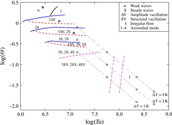
Regime diagram in the
 $({\it\Theta},Ta)$
plane established from experimental investigations (Wordsworth Reference Wordsworth2009); the control parameter values from the measurements are represented by open circles, and from the computations by filled circles along the line for
 ${\rm\Delta}T=2$
K. The traverses in dotted lines correspond to values obtained when varying the rotation rate at fixed temperature difference
 ${\rm\Delta}T$
(here 1 K, 2 K and 4 K). The continuous lines in blue indicate the transition between two flow regimes defined by different azimuthal dominant wavenumbers, while the dashed lines in red delimit the transition between two types of temporal dependence, and the two red dot-dashed lines delimit the transition zone between regular and irregular waves.

3. Results
The present work uses and extends the initial investigation concerned with the baroclinic instability by Randriamampianina & Crespo del Arco (Reference Randriamampianina, Crespo del Arco, von Larcher and Williams2014) and the preliminary analysis related to IGWs by Randriamampianina (Reference Randriamampianina2013).
Hide (Reference Hide1958), from his pioneering experimental investigations of baroclinic instability using liquids, has delineated three main classes of flow regimes: axisymmetric regimes, regular waves and irregular waves or geostrophic turbulence (see also Fowlis & Hide Reference Fowlis and Hide1965 and Hide & Mason Reference Hide and Mason1975). The regime where all perturbations decay to an axisymmetric flow is traditionally split into a lower symmetric (LS) regime, where the flow is strongly affected by viscous diffusion, and an upper symmetric (US) regime, where the flow is stabilized by stratification due to the background rotation. Despite the different labels and processes involved, no clear phase transition separates them. Experiments have also revealed the presence of the so-called ‘weak waves’ prior to the onset of regular waves (Hide & Mason Reference Hide and Mason1978; Castrejón-Pita & Read Reference Castrejón-Pita and Read2007; Wordsworth Reference Wordsworth2009).
However, one of the most intriguing problems comes from the mechanism responsible for the transition from regular waves to irregular waves. The regular wave regimes are composed of steady waves, denoted S, and vacillation regimes subdivided into amplitude vacillation, AV or MAV (modulated amplitude vacillation), and structural vacillation, SV. The steady waves are determined by a dominant azimuthal wavenumber
 $m$
in space, and characterized by periodic oscillations in time induced by the uniform angular drift of the waves with constant amplitude (such flows are denoted by
 $m\text{S}$
in figure 1). The amplitude vacillation regimes are defined by either periodic (AV), quasi-periodic or chaotic (MAV) temporal behaviour of the amplitude of the dominant wavenumber (see Read et al.
Reference Read, Bell, Johnson and Small1992 and Randriamampianina et al.
Reference Randriamampianina, Früh, Maubert and Read2006). The SV regime, an intermediate step before the transition towards geostrophic turbulence, is characterized by a spatio-temporal chaos but still with a well-defined dominant wavenumber, as pointed out by the experimental evidence of Früh & Read (Reference Früh and Read1997) (see also Read et al.
Reference Read, Maubert, Randriamampianina and Früh2008). In a previous paper (Read et al.
Reference Read, Maubert, Randriamampianina and Früh2008), direct numerical simulation in an air-filled baroclinic cavity has shown that small-scale fluctuations gradually break the regularity of the baroclinic waves, leading to the SV regime before the transition to geostrophic turbulence. This phenomenon was observed at high rotation rates, involving high values of the centrifugal acceleration in comparison with gravity, characterized by values of a local Froude number,
 $Fr_{r}={\it\Omega}^{2}r/g$
, larger than one everywhere inside the cavity. Therefore fluctuations were generated by rotating Rayleigh–Bénard-like instability in the radial direction, resulting from the application of the Boussinesq approximation to the centrifugal term (see (2.2)). Different behaviours are obtained in the present computations when using a liquid, and hence with a higher value of Prandtl number,
 $Pr=16$
, but where the Froude number remains small (
 $Fr_{r}\ll 1$
) for all rotation rates considered (see table 1).
The Prandtl number
 $Pr$
is a parameter of particular interest, also in the context of other convection problems (Gill & Davey Reference Gill and Davey1969). This can be easily understood through the ratio between the dynamical
 ${\it\delta}$
and thermal
 ${\it\delta}_{T}$
boundary layer thicknesses,
 ${\it\delta}/{\it\delta}_{T}=Pr^{1/3}$
. Then for air,
 $Pr=0.7$
,
 ${\it\delta}<{\it\delta}_{T}$
, unlike the behaviour for liquids, where
 $Pr>1$
. Fein & Pfeffer (Reference Fein and Pfeffer1976), who carried out a careful survey of the main flow regimes in a thermally driven rotating annulus using either mercury, water or silicon oils, found significant differences in the onset of baroclinic instability at low values of the Taylor number in the region of the so-called LS transition, where viscous and thermal diffusion terms are expected to play a major role. Hide (Reference Hide1958) mentioned that the transition from axisymmetric flow to regular waves at the US limit does not depend on the value of the Prandtl number but rather on the value of the thermal Rossby number with respect to an empirical critical value:
 ${\it\Theta}\leqslant {\it\Theta}_{c}=1.58\pm 0.05$
. Some substantial differences in the onset of various types of regular waves were noted at higher Taylor numbers. Jonas (Reference Jonas1981) investigated the influence of Prandtl number on the incidence of various forms of vacillation, using fluids with
 $Pr$
ranging from 11 to 74. He reported that amplitude vacillation, in particular, was significantly more widespread at high Prandtl number, though the onset of the ‘structural vacillation’ regime close to the transition zone at high Taylor number was less sensitive to
 $Pr$
. The Prandtl number was also found to play an important role in the occurrence of IGWs simultaneously with baroclinic instability. Indeed, from direct numerical simulations in a similar configuration, Jacoby et al. (Reference Jacoby, Read, Williams and Young2011) reported the presence of IGWs when using a liquid defined by
 $Pr=24$
, and recently so did Borchert et al. (Reference Borchert, Achatz and Fruman2014) with
 $Pr=7$
. On the other hand, in previous works with air,
 $Pr=0.7$
(Randriamampianina et al.
Reference Randriamampianina, Früh, Maubert and Read2006; Read et al.
Reference Read, Maubert, Randriamampianina and Früh2008), no emission of these small-scale fluctuations associated with baroclinic regular waves was observed.
The operating control parameters involved in the present simulations are plotted in figure 1 in a (
 ${\it\Theta},Ta$
) regime diagram established from experiments by Wordsworth (Reference Wordsworth2009). The slight difference between the measurements and the computations along the traverse at temperature difference
 ${\rm\Delta}T=2~\text{K}$
comes from the changes made to the experimental setup when drawing the diagram (
 $b_{exp}=14.3~\text{cm}$
, instead of the value
 $b=15~\text{cm}$
in the simulations, see Wordsworth (Reference Wordsworth2009)). However no significant differences were observed in the nature of the flow regime from the two approaches. In agreement with experimental findings, the first value at
 ${\it\Omega}=0.25~\text{rad}~\text{s}^{-1}$
, corresponding to
 $({\it\Theta},Ta)=(2.348,2.95\times 10^{6})$
, yields a weak wave flow while for the two others at
 ${\it\Omega}=0.35$
and
 $0.5125~\text{rad}~\text{s}^{-1}$
, located at
 $({\it\Theta},Ta)=(1.198,5.78\times 10^{6})$
and
 $(0.559,1.24\times 10^{7})$
in the regime diagram, the flow evolves to a regular wave regime, characterized temporally by an amplitude vacillation but with different dominant azimuthal wavenumbers: 2AV and 3AV, respectively. Even though measurements were not made at these specific values of the rotation rate, the regime diagram confirmed the nature of the computed flow regimes in the corresponding range of control parameters values, as clearly shown in figure 1.
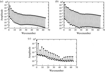
Spatial spectra of the time-averaged amplitudes of the azimuthal wave mode
 $m$
at mid-radius and mid-height of the cavity for the different values of
 ${\it\Omega}$
: (a)
 ${\it\Omega}=0.25~\text{rad}~\text{s}^{-1}$
; (b)
 $0.35~\text{rad}~\text{s}^{-1}$
; (c)
 $0.5125~\text{rad}~\text{s}^{-1}$
.

3.1. Background baroclinic flow
3.1.1. Weak waves
At the lowest value of rotation rate considered,
 ${\it\Omega}=0.25~\text{rad}~\text{s}^{-1}$
 $(Ta=2.95\times 10^{6})$
, the simulation predicts a ‘weak wave’ flow, with a dominant azimuthal wavenumber
 $m=2$
, in agreement with experimental findings, as can be seen in figure 1. Similarly to the observations of Castrejón-Pita & Read (Reference Castrejón-Pita and Read2007) from their experimental investigations in an air-filled cavity, the corresponding thermal Rossby number
 ${\it\Theta}=2.348$
is larger than the empirical critical value
 ${\it\Theta}_{c}=1.58\pm 0.05$
determined by Hide (Reference Hide1958) for the occurrence of the regular wave regime. This particular flow, developing prior to the onset of regular steady waves, is characterized by a small amplitude of the azimuthal variations of the temperature
 $A_{m}/{\rm\Delta}T<5\,\%$
(Hide & Mason Reference Hide and Mason1978), where the subscript
 $m$
refers to the dominant azimuthal wavenumber.
Figure 2 shows the time-averaged spatial spectra of the amplitude of the azimuthal wave mode of the temperature taken at mid-radius and at mid-height of the cavity
 $(r_{mid},z_{mid})$
from Fourier analysis. The dimensionless amplitude of the temperature for the dominant azimuthal wavenumber
 $m=2$
at
 ${\it\Omega}=0.25~\text{rad}~\text{s}^{-1}$
is
 $A_{2}=0.037$
, which can be considered as the normalized amplitude according to the scaling introduced for the temperature (
 ${\rm\Delta}T/2\equiv 1~\text{K}$
), and thus gives an actual amplitude 3.7 % of the imposed temperature difference. The amplitude calculated at the next higher rotation rate,
 ${\it\Omega}=0.35~\text{rad}~\text{s}^{-1}$
, is
 $A_{2}=0.12$
, which corresponds to the usual value linked to regular waves for large-Prandtl-number fluids (Fein & Pfeffer Reference Fein and Pfeffer1976). Furthermore an equivalent value of the amplitude
 $A_{3}=0.11$
was obtained at
 ${\it\Omega}=0.5125~\text{rad}~\text{s}^{-1}$
, characterized by a dominant azimuthal wavenumber
 $m=3$
. Similar behaviours have been mentioned by Castrejón-Pita & Read (Reference Castrejón-Pita and Read2007) from their experiments in an air-filled cavity, and by Hide & Mason (Reference Hide and Mason1978) when using liquids. It is worth recalling that the present solution is close to the transition from axisymmetric to non-axisymmetric flows at relatively high values of the Taylor number (see table 2).
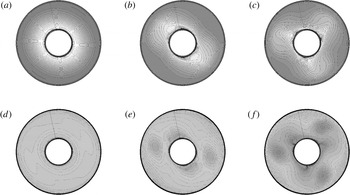
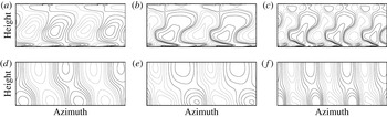
It was observed that the flow structure towards the upper half of the cavity remains broadly axisymmetric while the baroclinic waves are trapped towards the bottom of the cavity (figure 3). This is consistent with the observations of Hide & Mason (Reference Hide and Mason1978) with liquids, but in contrast with the flow pattern reported by Castrejón-Pita & Read (Reference Castrejón-Pita and Read2007), who found that the weak waves were visible at all heights of the cavity filled with air. This difference can be ascribed to thermal stratification levels resulting from the different fluid properties, namely the Prandtl number. In the case of air, the Prandtl number is one order of magnitude lower than for liquids, yielding a more uniform density gradient along the vertical direction than in liquids, where higher density gradient prevails in the lower part of the cavity. Castrejón-Pita & Read (Reference Castrejón-Pita and Read2007) suggested that this difference may come from a possible different physical origin of the two instabilities: barotropic for the air-filled cavity and fundamentally baroclinic for the liquid-filled cavity. Therefore the baroclinic instability first develops towards the bottom region in cavities filled with liquids.
Instantaneous isotherms for the three rotation rate values at different heights of the liquid-filled cavity: (a–c) at
 $z_{mid}=A/2=1.238$
, (d–f) at
 $z_{bot}=0.47$
, with
 $z\in [0,A]$
: (a,d)
 ${\it\Omega}=0.25~\text{rad}~\text{s}^{-1}$
; (b,e)
 $0.35~\text{rad}~\text{s}^{-1}$
; (c,f)
 $0.5125~\text{rad}~\text{s}^{-1}$
.

Another feature of the weak waves comes from their angular drift velocity relative to the cavity. Hide & Mason (Reference Hide and Mason1978) reported that weak waves drifted faster than the closest strong waves, even though the drift increases again with rotation rate for regular waves. Castrejón-Pita & Read (Reference Castrejón-Pita and Read2007) mentioned a ratio up to 10 between weak and strong waves in their air-filled experiment. In the present case, similar behaviour was also observed for the dimensionless drift frequency, with a ratio of 2.02 between the weak wave at
 ${\it\Omega}=0.25~\text{rad}~\text{s}^{-1}$
and the next strongest wave at
 ${\it\Omega}=0.35~\text{rad}~\text{s}^{-1}$
, and a ratio of 1.23 between the two regular waves with an increase of the drift with rotation rate. In dimensional values, since the reference time scale involves the rotation rate as
 $(2{\it\Omega})^{-1}$
, these ratios correspond to 1.44 and 1.19 respectively (see table 2).
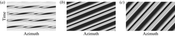
We have also detected significant differences in temporal behaviours between the weak and regular wave solutions when following the structures in the azimuthal direction with time. We have displayed in figure 4 the azimuth–time maps of the temperature taken at the centre of the cavity
 $(r_{mid},z_{mid})$
for the three rotation rates. It appears that the computed weak waves move like ‘pulsating’ azimuthally travelling waves. This can be ascribed to the faster drift of waves at
 ${\it\Omega}=0.25~\text{rad}~\text{s}^{-1}$
than at
 ${\it\Omega}=0.35~\text{rad}~\text{s}^{-1}$
: the ratio
 ${\it\omega}_{d}/{\it\Omega}$
for the weak wave is twice the value for the regular wave, where
 ${\it\omega}_{d}$
is the angular velocity drift of the baroclinic waves (see table 2). Indeed the pattern at
 ${\it\Omega}=0.25~\text{rad}~\text{s}^{-1}$
seems to remain in the azimuthal direction independently of the selected time length, unlike the regular waves at
 ${\it\Omega}=0.35$
and
 $0.5125~\text{rad}~\text{s}^{-1}$
with a characteristic slope, which varies as a function of the time duration considered for the map. We have used for
 ${\it\Omega}=0.25~\text{rad}~\text{s}^{-1}$
about
 $2\times T_{d}$
where
 $T_{d}$
is the dimensionless period of the wave drift,
 $T_{d}/2{\it\Omega}=2{\rm\pi}/{\it\omega}_{d}$
, while for
 ${\it\Omega}=0.35$
and
 $0.5125~\text{rad}~\text{s}^{-1}$
, it is about
 $2.5\times T_{d}$
and
 $1.5\times T_{d}$
respectively (see table 2 for the values of
 ${\it\omega}_{d}$
).
Azimuth–time map of the temperature at mid-radius and mid-height of the cavity for the three rotation rates: (a)
 ${\it\Omega}=0.25~\text{rad}~\text{s}^{-1}$
; (b)
 $0.35~\text{rad}~\text{s}^{-1}$
; (c)
 $0.5125~\text{rad}~\text{s}^{-1}$
.

Summary of computed results, with
 $m$
the dominant azimuthal wavenumber:
 ${\it\omega}_{d}$
is the drift frequency of baroclinic waves and
 ${\it\omega}_{v}$
the vacillation frequency (corresponding to the oscillations of the amplitude of the dominant azimuthal wavenumber).

These behaviours are consistent with the measurements of Hide & Mason (Reference Hide and Mason1978) in a liquid-filled cavity, keeping in mind that the computed solutions at
 ${\it\Omega}=0.25$
and
 $0.35~\text{rad}~\text{s}^{-1}$
are characterized by the same dominant wavenumber
 $m=2$
, while at
 ${\it\Omega}=0.5125~\text{rad}~\text{s}^{-1}$
, the dominant azimuthal wavenumber is
 $m=3$
. Both experimental investigations, using either liquids (Hide & Mason Reference Hide and Mason1978) or air (Castrejón-Pita & Read Reference Castrejón-Pita and Read2007), mentioned the marked transition between weak and strong waves. However, the baroclinic nature of the present computed flows has been clearly identified from the misalignment of eddy isobars with isotherms, as illustrated in figure 5. These eddy fields are obtained by removing the azimuthal flow corresponding to the azimuthally averaged field. This behaviour reflects the sloping convection reported by Hide & Mason (Reference Hide and Mason1975).
Instantaneous azimuth–height maps of the eddy fields (with azimuthal flow removed), (a–c) pressure, (d–f) temperature, for the three rotation rates: (a,d)
 ${\it\Omega}=0.25~\text{rad}~\text{s}^{-1}$
; (b,e)
 $0.35~\text{rad}~\text{s}^{-1}$
; (c,f)
 $0.5125~\text{rad}~\text{s}^{-1}$
.

3.1.2. Amplitude vacillation flow regime
At
 ${\it\Omega}=0.35$
and
 $0.5125~\text{rad}~\text{s}^{-1}$
, corresponding to
 $({\it\Theta},Ta)=(1.198,5.78\times 10^{6})$
and
 $(0.559,1.24\times 10^{7})$
in figure 1, the simulation predicts two regular wave flows characterized spatially by a dominant azimuthal wavenumber
 $m=2$
and
 $m=3$
, respectively, as shown in figures 2 and 3, and temporally by an amplitude vacillation. These solutions have been directly obtained by increasing progressively the rotation rate, e.g. the solution at the higher rotation rate was computed using as initial conditions the one at a lower rotation rate. The simulations were not able to capture any steady regular wave flow, although experiments reported 2S and 3S regimes in figure 1, recalling that the AV regime is obtained experimentally from steady waves by decreasing the rotation rate when using liquids
 $2\text{S}\rightarrow 2\text{AV}$
and
 $3\text{S}\rightarrow 3\text{AV}$
(Koschmieder & White Reference Koschmieder and White1981; Hignett et al.
Reference Hignett, White, Carter, Jackson and Small1985; Read et al.
Reference Read, Bell, Johnson and Small1992), unlike with air, which is by increasing rotation rate
 $2\text{S}\rightarrow 2\text{AV}\rightarrow 2\text{MAV}\rightarrow 3\text{S}$
(Randriamampianina et al.
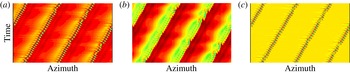
Reference Randriamampianina, Früh, Maubert and Read2006; Castrejón-Pita & Read Reference Castrejón-Pita and Read2007). Moreover, as soon as the regular baroclinic structures arose, we have observed the development of small-scale fluctuations initially along the cold inner cylinder, even though experimental studies did not mention such a behaviour. However, it can be ascribed to possible technical limitations in detecting the low level of these fluctuations (Read Reference Read1992). Thus, in some particular regions, the computed flow locally exhibits a spatio-temporal chaotic behaviour. We have presented in figure 6 the Hovmöller diagram in azimuth–time of the temperature at the onset of baroclinic instability for the three values of
 ${\it\Omega}$
at radius close to the inner cold cylinder and at height towards the bottom of the cavity
 $(r_{bl},z_{bot})$
(defined below). Starting from an axisymmetric solution, the spontaneous occurrence of small-scale features associated with the development of the large-scale baroclinic wave flow is seen, appearing as waves disturbances. However, these fluctuations clearly show a more prominent activity when increasing the rotation rate. The presence of these time-dependent fluctuations, discussed in following sections, indicates that the solution does not belong to the steady wave regime.
Azimuth–time map of the temperature at the onset of baroclinic instability for the different values of
 ${\it\Omega}$
at location
 $(r_{bl},z_{bot})$
: (a)
 ${\it\Omega}=0.25~\text{rad}~\text{s}^{-1}$
; (b)
 $0.35~\text{rad}~\text{s}^{-1}$
; (c)
 $0.5125~\text{rad}~\text{s}^{-1}$
.

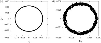
As already done by Randriamampianina et al. (Reference Randriamampianina, Früh, Maubert and Read2006) to describe the temporal characteristics, we use the representation in the phase-space based on time series of cosine and sine components of the dominant azimuthal wavenumber from Fourier analysis of the temperature at two specific fixed
 $(r,z)$
locations. We present these behaviours in figure 7 for
 ${\it\Omega}=0.5125~\text{rad}~\text{s}^{-1}$
, at which the intensity of the small-scale features is found to be the highest for the rotation rates considered. This was done long after the transient when the motion was fully established. In agreement with experimental findings of Wordsworth (Reference Wordsworth2009), figure 7(a) at mid-radius and mid-height of the cavity
 $(r_{mid},z_{mid})$
shows a classical 3AV profile defined by two frequencies: the wave drift represented by the large circle and the periodic oscillations of the wave amplitude, both related to the baroclinic instability (Randriamampianina et al.
Reference Randriamampianina, Früh, Maubert and Read2006). Figure 7(b), taken at radius location
 $r_{bl}$
inside the boundary layer along the inner cold cylinder and at height towards the bottom wall
 $z_{bot}$
, clearly exhibits a chaotic behaviour, referring to a 3MAV regime.
Phase-space diagrams for the temperature field at two fixed
 $(r,z)$
locations: (a)
 $(r_{mid},z_{mid})$
and (b) (
 $r_{bl},z_{bot}$
), for
 ${\it\Omega}=0.5125~\text{rad}~\text{s}^{-1}$
, showing the time series from Fourier analysis of the sine component
 $S_{3}$
against that of the cosine component
 $C_{3}$
of the azimuthal dominant mode
 $m=3$
.

Since such different AV regimes were not observed concurrently under fixed values of control parameters within the air-filled cavity (Randriamampianina et al.
Reference Randriamampianina, Früh, Maubert and Read2006) but successively when increasing the value of the rotation rate, this localized 3MAV solution is directly ascribed to the presence of small-scale features (see figure 6). These fluctuations, occurring spontaneously and simultaneously with the large-scale baroclinic waves, have been identified as inertia–gravity waves, IGWs (Jacoby et al.
Reference Jacoby, Read, Williams and Young2011). The magnitudes in figure 7 are related to IGW activity, more specifically to the balance between the two phenomena, with higher values associated with baroclinic instability. It reflects the variability of IGWs and the interaction between these very different waves scales, in time as well as in space. In particular, it puts forward the ability of the IGWs to locally induce a chaotic flow regime of the large-scale motion. Such a behaviour was not mentioned in descriptions of experiments (Wordsworth Reference Wordsworth2009). Moreover it clearly reveals the strong dependence on the Prandtl number of the baroclinic instability characteristics through the thermal stratification of the flow. These features cannot be attributed to the geometrical dimensions of the cavity, as we have obtained the same flow structures as reported by Randriamampianina et al. (Reference Randriamampianina, Früh, Maubert and Read2006) when using air in the present geometry, e.g. without any presence of these small-scale fluctuations. Finally, it is concluded that a steady wave regime cannot exist for liquids due to the presence of IGWs, but the non-axisymmetric flow enters directly into an AV regime. Früh & Read (Reference Früh and Read1997) reported from their experimental investigations using a liquid defined by
 $Pr=26$
that most of the observed wave-2 and wave-3 domains were time-dependent.
3.2. Identification of inertia–gravity waves at
 ${\it\Omega}=0.5125~\text{rad}~\text{s}^{-1}$

The analysis concerning the IGWs in the following sections is made for
 ${\it\Omega}=0.5125~\text{rad}~\text{s}^{-1}$
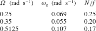
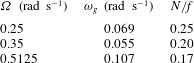
, which shows the highest intensity of fluctuations of the three rotation rates considered, as seen in figure 6. Some characteristics of the small-scale features are given in table 3 for the different rotation rates.
Some characteristics of IGWs for the different values of the rotation rate
 ${\it\Omega}$
:
 ${\it\omega}_{g}$
is the absolute frequency of IGWs in the rotating frame,
 $N$
is the buoyancy frequency and
 $f$
the Coriolis parameter.
To separate the two scales in time and in space of the fluctuations and the baroclinic waves, we introduce the three-term decomposition proposed by Hussain & Reynolds (Reference Hussain and Reynolds1970):
 $$\begin{eqnarray}f(\boldsymbol{X},t)=f^{\prime }(\boldsymbol{X},t)+\tilde{f}(\boldsymbol{X},t)+\overline{f}(\boldsymbol{X}),\end{eqnarray}$$
where
 $f$
represents each dependent variable of the flow,
 $\boldsymbol{X}$
is the position vector and
 $t$
denotes the time;
 $f^{\prime }$
corresponds to the fluctuations,
 $\tilde{f}$
to the large-scale structures and
 $\overline{f}$
to the time-averaged solution (see also Randriamampianina et al.
Reference Randriamampianina, Schiestel and Wilson2004).
Three-term decomposition in azimuth–time map of the temperature: (a)
 $T$
, (b)
 $\tilde{T}$
and (c)
 $T^{\prime }$
, at
 $(r_{bl},z_{bot})$
for
 ${\it\Omega}=0.5125~\text{rad}~\text{s}^{-1}$
: azimuth
 $0\leqslant {\it\theta}\leqslant 2{\rm\pi}$
and dimensionless time
 $0\leqslant t\leqslant 5600$
.

Temporal evolution at a fixed point, of (a) the temperature
 $T$
and (b) the corresponding fluctuations
 $T^{\prime }$
, with (c) an enlargement of the fluctuations, for
 ${\it\Omega}=0.5125~\text{rad}~\text{s}^{-1}$
.

To check its efficiency in capturing the different scales, the technique was applied to the azimuth–time map of the temperature at the location
 $(r_{bl},z_{bot})$
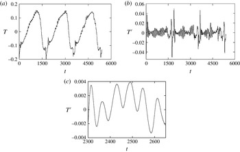
where the chaotic 3MAV behaviour was observed in figure 7. The three components are displayed in figure 8 for about three fundamental periods of the large-scale motion, showing the different waves structures and their strong links. From the temporal evolution plotted in figure 9, we can deduce the dimensionless periods in the reference frame rotating with the cavity,
 $T_{d}=T_{d}^{\ast }\times 2{\it\Omega}\sim 1800$
and
 $T_{g}=T_{g}^{\ast }\times 2{\it\Omega}\sim 60$
, giving the dimensional drift frequency
 ${\it\omega}_{d}^{\ast }=2{\rm\pi}/T_{d}^{\ast }\sim 3.578\times 10^{-3}~\text{rad}~\text{s}^{-1}$
for the large-scale background flow and absolute frequency
 ${\it\omega}_{g}^{\ast }=2{\rm\pi}/T_{g}^{\ast }\sim 0.107~\text{rad}~\text{s}^{-1}$
for the fluctuations, respectively (
 $^{\ast }$
denotes dimensional variables, and
 $(2{\it\Omega})^{-1}$
is the reference time scale). It is worth mentioning the characteristic stiff jump of the temperature during AV regimes (Randriamampianina et al.
Reference Randriamampianina, Früh, Maubert and Read2006), which is reflected in the evolution of the fluctuations. Note the difference of time scales between the two phenomena,
 $T_{d}/T_{g}\sim 30$
, as well as of the amplitudes of oscillations.
To determine the nature of these small-scale features, this absolute frequency
 ${\it\omega}_{g}^{\ast }$
obtained from computations can be compared with another value provided independently from the Doppler effect, involving the intrinsic frequency calculated from the IGW dispersion relation. This frequency corresponds to the one that would be observed in a frame moving with the background flow. The dispersion relation can be written (Gill Reference Gill1982; Fritts & Alexander Reference Fritts and Alexander2003) (dropping the *)
 $$\begin{eqnarray}\hat{{\it\omega}}^{2}=\frac{N^{2}(k^{2}+l^{2})+f^{2}m^{2}}{k^{2}+l^{2}+m^{2}},\end{eqnarray}$$
where
 $N=\sqrt{g{\it\alpha}\partial T/\partial z}$
is the buoyancy frequency,
 $f=2{\it\Omega}$
is the Coriolis parameter, and
 $k,l,m$
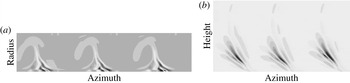
are the wavenumbers in the radial, zonal and vertical directions. Similarly to the frequencies, the wavenumbers can be estimated from cross-sections of instantaneous fluctuation fields (figure 10). The horizontal velocity divergence
 $\boldsymbol{{\rm\nabla}}_{H}\boldsymbol{\cdot }\boldsymbol{V}$
, presented in the azimuth–height map of figure 10(b), is commonly used to give a measure of the intensity of IGWs. Then, applying the same approach as used by Jacoby et al. (Reference Jacoby, Read, Williams and Young2011) in a similar configuration, we have estimated the dimensional values of the wavenumbers as
 $(k,l,m)\sim (5.27~\text{cm}^{-1},5.4~\text{cm}^{-1},1.45~\text{cm}^{-1})$
. The value of the zonal wavenumber
 $l$
was taken at radial distance
 $r_{bl}\sim 5~\text{cm}$
, corresponding to the radial location of the highest intensity of fluctuations.
 $N\sim 0.17~\text{rad}~\text{s}^{-1}$
is estimated from the mean temperature gradient
 ${\rm\Delta}T/{\rm\Delta}z\sim 0.1~\text{K}~\text{cm}^{-1}$
in the region where IGWs prevail, while
 $f=1.025~\text{rad}~\text{s}^{-1}$
, giving
 $N/f\sim 0.17$
. Finally from (3.2) we obtain
 $\hat{{\it\omega}}\sim 0.26~\text{rad}~\text{s}^{-1}$
(see Randriamampianina Reference Randriamampianina2013).
Instantaneous fields in different planes for
 ${\it\Omega}=0.5125~\text{rad}~\text{s}^{-1}$
: (a)
 $T^{\prime }({\it\theta},r)$
at
 $z_{bot}$
with
 ${\it\theta}\in [0,2{\rm\pi}]$
and
 $r\in [0.3,1]$
, and (b)
 $\boldsymbol{{\rm\nabla}}_{H}\boldsymbol{\cdot }\boldsymbol{V}({\it\theta},z)$
at
 $r_{bl}$
with
 $z\in [0,A=2.476]$
.

These characteristics,
 $N<\hat{{\it\omega}}<f$
, with
 $\hat{{\it\omega}}\sim N<f$
, are consistent with the findings of Jacoby et al. (Reference Jacoby, Read, Williams and Young2011), described by
 $N/f\sim 0.12$
. This is in contrast with the behaviour observed in the real atmosphere and oceans where
 $f<\hat{{\it\omega}}<N$
. In their numerical simulations studying these ranges of frequencies with their ‘atmosphere-like’ model where
 $N/f>1$
, Borchert et al. (Reference Borchert, Achatz and Fruman2014) reported the occurrence of IGWs propagating along the inner cold cylinder, similarly to the features observed by Jacoby et al. (Reference Jacoby, Read, Williams and Young2011) and in the present work. They also mentioned the development of additional IGWs toward the interior of the cavity, almost stationary with respect to the baroclinic waves and found to originate from spontaneous gravity wave emission. These authors obtained a strongly stratified flow configuration with
 $N/f\sim 4$
for shallow water, using
 $(b-a)/d>1$
associated with a small value of the Coriolis parameter and a large temperature difference. Indeed, in the atmosphere and oceans, the horizontal extent is very large compared with the vertical distance, combined with small value of the Coriolis parameter, with typically
 $N/f\sim 100$
.
Then we can deduce another absolute frequency,
 ${\it\omega}_{a}$
, for the fluctuations using the Doppler relation (Jacoby et al.
Reference Jacoby, Read, Williams and Young2011):
 $$\begin{eqnarray}{\it\omega}_{a}=\hat{{\it\omega}}-l\,\overline{v},\end{eqnarray}$$
since the motion of the background flow corresponds to the uniform drift of the baroclinic waves in the zonal direction:
 $\overline{v}=r_{bl}{\it\omega}_{d}$
. We find that
 ${\it\omega}_{a}\sim 0.16~\text{rad}~\text{s}^{-1}$
, which is to be compared with the computed value
 ${\it\omega}_{g}\sim 0.107~\text{rad}~\text{s}^{-1}$
. The consistency of these values confirms the nature of these small-scale features to be IGWs. Exact agreement cannot be obtained due in particular to the waves variability, keeping in mind that wavenumbers have been estimated from instantaneous fields characterized by chaotic behaviour. The intrinsic frequency can be also affected by the non-uniformity of the flow in the vertical direction. For instance, the vertical shear and the variation of
 $N$
in the vertical direction modify the intrinsic frequency and the phase velocity, as has been stated by Booker & Bretherton (Reference Booker and Bretherton1967) (see also Staquet & Sommeria Reference Staquet and Sommeria2002). We will see in following sections that the flow has both features. Moreover, the dispersion relation (3.2) has been established from linear analysis, but nonlinear terms play a key role during the development of the present time-dependent flows.
3.3. Wave parameters
In an unbounded stratified fluid, the inertia–gravity waves may propagate vertically as well as horizontally. Defining the angle
 ${\it\varphi}$
of the wavenumber vector,
 $\boldsymbol{K}=(k,l,m)$
, with the horizontal, we can write (Gill Reference Gill1982)
 $$\begin{eqnarray}\displaystyle m=K\sin {\it\varphi},\quad {\it\kappa}_{H}=K\cos {\it\varphi}, & & \displaystyle\end{eqnarray}$$
where
 ${\it\kappa}_{H}=(k^{2}+l^{2})^{1/2}$
is the magnitude of the horizontal wavenumber vector,
 $\boldsymbol{k}_{H}=(k,l)$
, and
 $K=({\it\kappa}_{H}^{2}+m^{2})^{1/2}$
the magnitude of the wavenumber vector. Then the dispersion relation may be rewritten as
 $$\begin{eqnarray}\hat{{\it\omega}}^{2}=N^{2}\cos ^{2}{\it\varphi}+f^{2}\sin ^{2}{\it\varphi}.\end{eqnarray}$$
The phase velocity vector is directed along
 $\boldsymbol{K}$
whereas the group velocity is perpendicular to
 $\boldsymbol{K}$
. The aspect ratio of the phase velocity vector is (Gill Reference Gill1982)
 $$\begin{eqnarray}\frac{\text{vertical scale}}{\text{horizontal scale}}=\frac{{\it\kappa}_{H}}{m}=\sqrt{\frac{f^{2}-\hat{{\it\omega}}^{2}}{\hat{{\it\omega}}^{2}-N^{2}}}=\cot {\it\varphi}.\end{eqnarray}$$
By using the known values of the wavenumbers
 $k,l,m$
, we obtain the angle
 ${\it\varphi}\approx 11^{\circ }$
.
3.3.1. Wave regimes
In oceans and atmosphere the stratification is more important than the rotation rate, the representative parameters being commonly
 $N\geqslant \hat{{\it\omega}}\geqslant f$
(typically
 $N/f\sim 100$
).
In the present baroclinic cavity
 $f>N$
and the dispersion relation can be rewritten as
 $$\begin{eqnarray}\frac{m^{2}}{{\it\kappa}_{H}^{2}}=\frac{\hat{{\it\omega}}^{2}-N^{2}}{f^{2}-\hat{{\it\omega}}^{2}}.\end{eqnarray}$$
Then in the limit
 $m^{2}<{\it\kappa}_{H}^{2}$
, the different regimes in this range can be delineated as follows (Gill Reference Gill1982; Fritts & Alexander Reference Fritts and Alexander2003).
-
(1) High-frequency regime (
$\hat{{\it\omega}}\sim f$
but
$\hat{{\it\omega}}\leqslant f$
): in this case
$N^{2}$
is negligible in comparison with
$\hat{{\it\omega}}^{2}$
in the numerator of the dispersion relation (3.7), which reduces to (3.8)
$$\begin{eqnarray}\hat{{\it\omega}}\cong \left[\frac{f^{2}\,m^{2}}{m^{2}+{\it\kappa}_{H}^{2}}\right]^{1/2}.\end{eqnarray}$$
-
(2) Low-frequency regime (
$\hat{{\it\omega}}\sim N$
but
$\hat{{\it\omega}}\geqslant N$
): in this regime
$\hat{{\it\omega}}^{2}$
can be neglected in comparison with
$f^{2}$
in the dispersion relation, which becomes (3.9)
$$\begin{eqnarray}\hat{{\it\omega}}\cong \left[N^{2}+\frac{f^{2}m^{2}}{{\it\kappa}_{H}^{2}}\right]^{1/2}.\end{eqnarray}$$
-
(3) Mid-frequency regime (
$f\gg \hat{{\it\omega}}\gg N$
): the dispersion relation simplifies to (3.10)
$$\begin{eqnarray}\hat{{\it\omega}}\cong \left[f^{2}\frac{m^{2}}{{\it\kappa}_{H}^{2}}\right]^{1/2}.\end{eqnarray}$$


The analytical solution derived from linear theory
 $\hat{{\it\omega}}(m)$
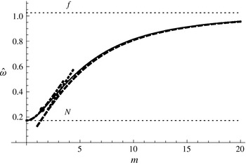
is plotted in figure 11 with the three approximations to the frequency regimes in (3.8)–(3.10). As
 $f$
is greater than
 $N$
, but not by too much, the three regimes are not fully developed. The characteristics of the wave packet are represented in figure 11 with a filled circle; thus the IGWs fit very well with the low-frequency regime approximation
 $\hat{{\it\omega}}\sim N$
. In these low-frequency inertia waves the stratification plays an important role. For small vertical wavenumber (waves long compared with the horizontal wavelength) the frequency
 $\hat{{\it\omega}}$
is only slightly above the Brunt–Väisälä frequency,
 $N$
. For larger vertical wavenumbers the waves are affected by gravity and are governed by the inertial wave dispersion relation for a non-stratified medium.
The dispersion relation for internal waves,
 $\hat{{\it\omega}}(m)$
is represented with a continuous thin line. The approximations for the different regimes are indicated with a long-dashed line (high-frequency regime), a short-dashed line (medium-frequency regime) and a dot-dashed line (low-frequency regime). The filled circle represents the internal wave obtained at
 ${\it\Omega}=0.5125~\text{rad}~\text{s}^{-1}$
. The horizontal lines represent the values at
 $f=2{\it\Omega}$
and
 $N=0.17~\text{rad}~\text{s}^{-1}$
.

3.3.2. Group velocity direction
The dispersion relation is written
 $$\begin{eqnarray}\hat{{\it\omega}}=\sqrt{\frac{f^{2}m^{2}+N^{2}{\it\kappa}_{H}^{2}}{{\it\kappa}_{H}^{2}+m^{2}}}\end{eqnarray}$$
and the intrinsic group velocity is
 $$\begin{eqnarray}\boldsymbol{c}_{\boldsymbol{g}}=\frac{1}{\hat{{\it\omega}}\,K^{2}}[\boldsymbol{e}_{z}m(f^{2}-\hat{{\it\omega}}^{2})-\boldsymbol{k}_{H}(\hat{{\it\omega}}^{2}-N^{2})].\end{eqnarray}$$
Using (3.9) the vertical component of the group velocity can be rewritten as
 $$\begin{eqnarray}{\hat{c}}_{gz}=\frac{\hat{{\it\omega}}}{m}\left(1-\frac{N^{2}}{\hat{{\it\omega}^{2}}}\right).\end{eqnarray}$$
Note that here the vertical group velocity,
 ${\hat{c}}_{gz}$
, and the vertical phase velocity,
 ${\hat{c}}_{pz}=\hat{{\it\omega}}/m$
, have the same sign, while in the more common situations like the atmosphere and the oceans where
 $N\gg f$
they are in opposite directions. Then, in this case an inertia–gravity wave propagating upward, with positive
 ${\hat{c}}_{gz}$
, has upward phase propagation.
The slope of constant phase lines is
 ${\it\kappa}_{H}/m=\cot {\it\varphi}$
, with
 ${\it\varphi}\approx 11^{\circ }$
.
The ratio of horizontal to vertical group velocity in the low-frequency regime defined in (3.9),
 $$\begin{eqnarray}\left|\frac{{\hat{c}}_{gH}}{{\hat{c}}_{gz}}\right|=\left|\frac{m}{{\it\kappa}_{H}}\right|\approx \frac{(\hat{{\it\omega}}^{2}-N^{2})^{1/2}}{f},\end{eqnarray}$$
is small relatively to its high-frequency counterpart. This regime is equivalent to the low-frequency regime observed in the ocean and atmosphere (Gill Reference Gill1982; Fritts & Alexander Reference Fritts and Alexander2003), where
 $f\ll N$
and
 $\hat{{\it\omega}}\cong f$
, associated with a large horizontal extent compared with the vertical distance. In the present case the low-frequency regime is attained when
 $\hat{{\it\omega}}\cong N$
and from (3.14) associated with a large horizontal extent compared with the vertical distance. Then
 ${\it\kappa}_{H}\ll m$
means that inertia–gravity waves can be found at large horizontal distances from the sources. In the present case with
 $f>N$
, the small value of the ratio of the group velocity components yields
 ${\hat{c}}_{gH}\ll {\hat{c}}_{gz}$
; thus the IGWs in this regime can be transmitted to large vertical distances from their source.
In the top region of the cavity, the increasing distance between the isolines of the temperature field reveals that
 $N$
tends to zero for increasing radius (see the instantaneous isotherms
 $T(r,z)$
displayed in figure 14 below). Then the dispersion relation formulated in (3.5) yields
 $\hat{{\it\omega}}\approx f\sin {\it\varphi}$
and from (3.12) we have
 $$\begin{eqnarray}\displaystyle |{\hat{c}}_{g}|=\frac{f\cos {\it\varphi}}{K}. & & \displaystyle\end{eqnarray}$$
The energy propagation is vertical in this zone,
 ${\it\varphi}\approx 0$
but
 $|{\hat{c}}_{g}|\neq 0$
, and the flow is steady in the rotating reference frame attached to the cavity,
 $\hat{{\it\omega}}\approx 0$
. In this situation the energy is concentrated in the cone whose apex angle is
 ${\it\varphi}$
, and the onset of three stagnation zones relative to the steady source at the bottom is observed, corresponding to Taylor columns (see LeBlond & Mysak Reference LeBlond and Mysak1978) as illustrated in figure 10(b).
3.3.3. Polarization relations
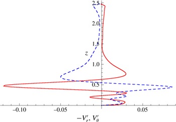
The polarization relationships between the variables characterizing IGWs are obtained by substituting the wave form in the relevant governing equations for the linear flow, i.e. neglecting viscosity and thermal diffusivity terms as well as nonlinear terms (Fritts & Alexander Reference Fritts and Alexander2003). The axial variations of the computed fluctuations of the meridional velocity
 $-V_{r}^{\prime }$
and of the zonal velocity
 $V_{{\it\theta}}^{\prime }$
are displayed in figure 12, at fixed
 $(r,{\it\theta})$
location corresponding to highest level of IGWs. We can clearly see that both maximum absolute values occur at
 $z_{bot}=0.47$
, revealing the location of highest intensity of IGWs. Note that the thickness of the Ekman boundary layer along the horizontal walls is about
 ${\it\delta}_{E}\approx \sqrt{{\it\nu}/{\it\Omega}}\approx 0.2~\text{cm}$
, which corresponds to a dimensionless value
 $z_{E}\approx 0.02$
, with
 $z\in [0,A=2.476]$
.
Instantaneous axial variation of the fluctuations of the meridional velocity
 $-V_{r}^{\prime }$
(red, solid), and of zonal velocity
 $V_{{\it\theta}}^{\prime }$
(blue, dashed) for
 ${\it\Omega}=0.5125~\text{rad}~\text{s}^{-1}$
, at an
 $(r,{\it\theta})$
location where the intensity of the gravity wave is highest (
 $z\in [0,A=2.476]$
).

The linear theory provides polarization equations for the variables (see Fritts & Alexander Reference Fritts and Alexander2003), including the background wind effects. The relationship between
 $V_{r}^{\prime }$
and
 $V_{{\it\theta}}^{\prime }$
for constant background wind
 $\boldsymbol{U}$
, is written
 $$\begin{eqnarray}-\!V_{r}^{\prime }=\frac{\text{i}{\it\omega}_{g}k+f\hspace{0.0pt}l}{\text{i}{\it\omega}_{g}l-fk}V_{{\it\theta}}^{\prime }.\end{eqnarray}$$
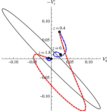
The hodograph in figure 13 represents the meridional velocity fluctuations
 $-V_{r}^{\prime }$
versus the zonal velocity fluctuations
 $V_{{\it\theta}}^{\prime }$
taken from figure 12, together with the theoretical ellipse drawn from the polarization relationship in (3.16). The elliptical shape of the hodograph is recognized to be a signature of IGWs (Tateno & Sato Reference Tateno and Sato2008). The main ellipse is turning clockwise with height indicating a vertically upward propagation in the region
 $0.4<z<1.8$
, delimiting the location of IGW activity pointed out in figure 12. For
 $z<0.4$
and for
 $z>1.8$
the ellipse rotates counterclockwise and the wave travels downward,
 ${\hat{c}}_{gz}<0$
and
 ${\hat{c}}_{pz}<0$
. Thomas et al. (Reference Thomas, Worthingthon and McDonald1999) reported a similar change in the atmosphere, where hodographs of the fluctuations reveal that the wave moves upward below the tropopause and downward above.
Polarization relation representing instantaneous meridional velocity
 $-V_{r}^{\prime }$
versus zonal velocity
 $V_{{\it\theta}}^{\prime }$
for
 ${\it\Omega}=0.5125~\text{rad}~\text{s}^{-1}$
. The polarization relation from linear theory is represented with a black continuous line. The hodograph rotates clockwise with height in
 $z\in [0.4,1.8]$
, indicating upward energy propagation (red line), and counterclockwise in the zones
 $z>1.8$
and
 $z<0.4$
(blue lines).

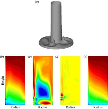
(a) Instantaneous isosurface of the total temperature, and (b–e) three-term decomposition of the temperature field at fixed azimuth
 ${\it\theta}$
, together with the time-averaged temperature field, for
 ${\it\Omega}=0.5125~\text{rad}~\text{s}^{-1}$
: (b)
 $T(r,z)$
, (c)
 $\tilde{T}(r,z)$
, (d)
 $T^{\prime }(r,z)$
and (e)
 $\bar{T}(r,z)$
.

The orientation of the major axis of the hodograph’s ellipse in figure 13 corresponds to that of the wavenumber with an
 $180^{\circ }$
ambiguity, and the direction of vertical energy propagation of the IGWs is obtained from the rotation of the hodograph ellipses: clockwise (anticlockwise) rotation with height indicates upward (downward) propagation.
3.4. Generation mechanism
For the same kind of IGWs, Jacoby et al. (Reference Jacoby, Read, Williams and Young2011) concluded that a localized boundary layer instability was the generation mechanism, irrespective of the rotation effect involved and therefore of the baroclinic instability. In the present simulation, the IGWs clearly remain attached to the baroclinic waves, as illustrated in figures 6–8. According to the theoretical study by Gill & Davey (Reference Gill and Davey1969), the values of parameters considered in the present simulation, such as the Rayleigh number, the Prandtl number and the aspect ratio, should lead to the development of such a buoyancy layer instability, as discussed later. The present IGWs were observed spreading from the inner cold cylinder, appearing in the form of a ‘hook’, following the baroclinic wave-3 structure for
 ${\it\Omega}=0.5125~\text{rad}~\text{s}^{-1}$
, as revealed by the instantaneous isotherms in an
 $(r,{\it\theta})$
plane taken towards the bottom wall of the cavity (see figure 3). We can also clearly see the presence of three ‘extra outgrowths’ of cold fluid just outside the cyclonic vortices, attached to the baroclinic waves, involving another instability. These phenomena are also visible in the temperature field obtained for the regular wave flow 2AV at
 ${\it\Omega}=0.35~\text{rad}~\text{s}^{-1}$
in figure 3 at the same height
 $z_{bot}$
. These features were not observed during the simulation of baroclinic instability within an air-filled cavity.
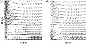
Enlargement of the velocity field towards the bottom wall in an
 $(r,z)$
plane for
 ${\it\Omega}=0.5125~\text{rad}~\text{s}^{-1}$
, with
 $0.3\leqslant r\leqslant 0.65$
and
 $0\leqslant z\leqslant 0.9$
: (a) total flow; (b) large-scale baroclinic flow (the cold wall is at the left, and
 $(r,z)\in [0.3,1]\times [0,A=2.476]$
).

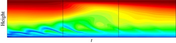
The small-scale fluctuations propagate vertically along the inner cold wall over three ridges following the baroclinic wave-3 flow, as seen from an instantaneous isosurface of the temperature (figure 14). The intensity decreases with height, as the IGWs are absorbed by the hot zone dominating the upper region of the cavity, conspicuous on the instantaneous temperature field
 $T(r,z)$
shown in figure 14, where
 $\hat{{\it\omega}}\rightarrow N$
and
 $m\rightarrow 0$
giving rise to Taylor columns (LeBlond & Mysak Reference LeBlond and Mysak1978), as illustrated in figure 10(b) where the wavenumber vector becomes horizontal. These Taylor columns result from the excitation of the baroclinic waves by the IGWs. This is supported by the behaviour of the group velocity, with a change of direction near
 $z=1.8$
to become a Taylor column (see figure 13). Intense activity of IGWs prevails towards the bottom wall due to the high value of
 $Pr$
, with a strong stratification, while toward the top part of the cavity the characteristics of the IGW develop to almost inertial waves with vertical propagation. Just before the emission of IGWs along the inner cylinder, represented by the broken isosurface, a density overturn was observed, as shown by the presence of the outgrowth of cold fluid outside the baroclinic waves revealed by
 $T(r,{\it\theta})$
in figure 3 and of a hump on the isosurface in figure 14. To determine the nature of this new instability the Richardson number, defined by
 $$\begin{eqnarray}\displaystyle Ri=\frac{N^{2}}{(\partial V_{{\it\theta}}/\partial z)^{2}}, & & \displaystyle\end{eqnarray}$$
has been calculated and found to satisfy the criterion
 $Ri\sim 0.20<Ri_{c}=0.25$
in this zone, a necessary condition for the onset of a localized Kelvin–Helmholtz instability (KHI).
We have displayed in figure 14 the instantaneous fields of the three components of the temperature in an
 $(r,z)$
plane at fixed azimuth, resulting from the three-term decomposition defined in (3.1). The time-averaged temperature field is also presented. We can see the occurrence of the IGWs along the inner cold cylinder, but also just before, a thickening of the horizontal boundary layer induced by the presence of an overturn of temperature visible in the large-scale background baroclinic field
 $\tilde{T}$
towards the bottom wall. This is represented by the aforementioned outgrowth of cold fluid in the
 $(r,{\it\theta})$
plane. However, this is not observed in the fluctuations of temperature
 $T^{\prime }(r,z)$
, which mainly exhibit the IGWs along the cold inner cylinder. Note that the height
 $z_{bot}$
corresponds to the vertical location of the upper ‘red bubble’, and the IGWs structure is to be connected to the axial profiles of radial and zonal components of the velocity fluctuations displayed in figure 12. An enlargement of the velocity field in the meridional plane
 $(r,z)$
in the region showing the IGWs and the temperature overturn is presented in figure 15 for the total and the large-scale flows. The large-scale baroclinic velocity field exhibits a flow reversal associated with a stagnation point located along the horizontal boundary layer toward the inner cold wall. The KHI occurs at this stagnation point and then gives rise to IGWs when arriving at the vertical wall. The IGWs appear along the inner cold cylinder at the meeting of the strong advected flow directed downward with the reversed flow moving upward along this wall. This scenario is consistent with the theoretical study by Lott et al. (Reference Lott, Kelder and Teitelbaum1992) in an unbounded stratified shear layer. These authors mentioned that Kelvin–Helmholtz instability in a shear layer can develop propagating waves in the presence of a rigid wall, invoking resonant over-reflection, as the present IGWs are also characterized by
 $Ri<0.25$
(Lindzen Reference Lindzen1974; Lindzen & Rosenthal Reference Lindzen and Rosenthal1976), as can be seen later.
The time–height map of the temperature, displayed in figure 16 at this fixed azimuth and radius location corresponding to the stagnation point in the large-scale baroclinic flow (outside the boundary layer), shows the characteristic detached layer of KHI, oscillating with the same (dimensionless) period as the IGWs with
 $T_{KH}\sim 60$
. The temperature overturn is clearly seen. The oscillations are not damped but the instability is transported by the drifting background wave-3 flow, similarly to the IGWs. This behaviour still confirms the strong links of these instabilities with the large-scale baroclinic motion. Such a shear layer instability along the horizontal bottom wall may be associated with the stronger stratification induced by the high Prandtl number value
 $Pr=16$
combined with the confinement with an aspect ratio
 $(b-a)/d<1$
and especially with the insulating boundary condition imposed at this wall.
Time–height map of the temperature at a fixed
 $(r,{\it\theta})$
location for
 ${\it\Omega}=0.5125~\text{rad}~\text{s}^{-1}$
: dimensionless time
 $0\leqslant t\leqslant 540$
, and
 $0\leqslant z\leqslant A=2.476$
.

During their simulation of large-scale atmospheric circulation in a spherical cavity, O’Sullivan & Dunkerton (Reference O’Sullivan and Dunkerton1995) mentioned that KHI was responsible for the breakdown of IGWs associated with baroclinic waves. As observed in figure 7, the present IGWs have locally triggered a spatio-temporal chaotic flow regime. The IGW emission is different from the behaviour obtained by Plougonven & Snyder (Reference Plougonven and Snyder2007) from simulations of idealized baroclinic life cycles, where the IGWs develop at the exit of the jet generated by the shear between the cyclonic and anticyclonic parts. The latter flow is characterized by a higher stratification level compared with inertial frequency,
 $N\gg f$
, and associated with an aspect ratio (horizontal extent/vertical distance)
 $\gg$
1. Borchert et al. (Reference Borchert, Achatz and Fruman2014) reported the occurrence of similar IGWs in their ‘atmosphere-like’ configuration, which may be also ascribed to the presence of an open upper free surface, unlike in the present configuration where the top is covered by a rigid lid. When using air (
 $Pr=0.7$
) as working fluid in the present cavity, we did not observe any occurrence of IGWs, confirming the important role played by the Prandtl number through the stratification.
4. Discussion
A survey of the gravity wave sources, including references using different methodologies, is provided by Fritts & Alexander (Reference Fritts and Alexander2003) and more recently by Plougonven & Zhang (Reference Plougonven and Zhang2014). The proposed sources for inertia–gravity wave generation include mainly topography, wind shear, convection and geostrophic adjustment. While unstable shear zones in the flow radiate waves with phase speeds equal to the flow speed in shear zones, waves forced by topography are associated with phase speeds close to zero.
We have studied the properties of two unstable shear zones in the flow: the boundary layer developing along the inner cylindrical wall and the shear induced by the periodic passing of the baroclinic wave. The instability of the boundary layer flow along the inner cylindrical wall was suggested by Jacoby et al. (Reference Jacoby, Read, Williams and Young2011) to be the origin of the IGWs. The formation of a mixed layer of fluid by the passing of the baroclinic wave and the emission of shear-generated IGWs as a consequence are explored in this section.
The flow and the stratification vary inside the cavity and undergo changes due to the baroclinic waves. We will attempt to determine the characteristics and the propagation of the wave in order to see whether it is reasonable to postulate the aforementioned phenomena as the source of the IGWs.
4.1. Instability of the boundary layer in a buoyancy-driven system
According to the theoretical results of Gill & Davey (Reference Gill and Davey1969), the stability of the boundary layer may be estimated using the width of the boundary layer
 $\ell$
and the associated vertical velocity
 $W$
, defined as
 $$\begin{eqnarray}\displaystyle & \displaystyle \ell ^{2}=2({\it\nu}{\it\kappa})^{1/2}/N, & \displaystyle\end{eqnarray}$$
 $$\begin{eqnarray}\displaystyle & \displaystyle W={\it\alpha}g{\rm\Delta}T/Pr^{1/2}N. & \displaystyle\end{eqnarray}$$
The estimated value of the Brunt–Väisälä frequency in the present configuration is
 $N\sim 0.17~\text{rad}~\text{s}^{-1}$
. Equations (4.1), (4.2) provide the values of the boundary layer width and of the vertical velocity:
 $$\begin{eqnarray}\displaystyle \ell =0.24\text{ cm}\quad \text{and}\quad W=0.89\text{ cm s}^{-1}. & & \displaystyle\end{eqnarray}$$
Then a theoretical Reynolds number can be deduced (Gill & Davey Reference Gill and Davey1969):
 $$\begin{eqnarray}\displaystyle Re=\frac{W\ell }{{\it\nu}}=\frac{{\it\alpha}g{\rm\Delta}T\ell ^{3}}{2{\it\nu}^{2}}=10.5. & & \displaystyle\end{eqnarray}$$
From figure 3 of Gill & Davey (Reference Gill and Davey1969) the stability boundary layer graphics predicts a critical value
 $Re_{c}\approx 5$
for a value of the Prandtl number,
 $Pr=20$
, close to the one considered in the present study.
The characteristics of the wave packet found in the present numerical results can be compared with the characteristics of the boundary layer instability near threshold provided in table 1 of Gill & Davey (Reference Gill and Davey1969). For
 $Pr=20$
and
 $Re_{c}=5$
the critical wavenumber predicted is approximately
 $0.46/\ell \approx 2~\text{cm}^{-1}$
and the frequency of the travelling wave at the threshold is about
 $0.033~\text{rad}~\text{s}^{-1}$
. In the present computations, with
 $Pr=16$
and
 $Re=10.5$
the characteristic values of the wave packet correspond to
 ${\it\omega}_{g}\approx 0.1~\text{rad}~\text{s}^{-1}$
and
 $1.5~\text{cm}^{-1}$
for the vertical component of the wavenumber. These values are thus of the same order, suggesting that the boundary layer instability may be a candidate for a generation mechanism of the inertia–gravity waves. However, it is clearly seen that the IGWs remain attached to the large-scale background baroclinic waves. Even though the interaction between the two phenomena is not yet clearly understood, it was observed that IGWs locally trigger chaotic motion of the background large-scale baroclinic waves. Therefore it is thought that the computed IGWs are different from the travelling waves obtained by Gill & Davey (Reference Gill and Davey1969) in their theoretical study. Moreover, in a subsequent analytical study, Bergholz (Reference Bergholz1978) mentioned that, when the temperature difference is greater than a certain critical value, ‘the critical disturbance modes are stationary when
 $Pr<12.7$
, but they are travelling waves when
 $Pr\geqslant 12.7$
’, corresponding to IGWs. Therefore the presence of IGWs in water-filled cavity (
 $Pr=7$
), as recently reported by Borchert et al. (Reference Borchert, Achatz and Fruman2014), should suggest that this localized boundary layer instability is not the generation mechanism of IGWs within the present baroclinic cavity. Moreover, the instabilities investigated by Gill & Davey (Reference Gill and Davey1969) are purely two-dimensional, while in the present study, the solution exhibits three-dimensional characteristics. In particular, the azimuthal wavenumber of the observed IGWs is similar in value to the radial wavenumber in the present study as well as in Jacoby et al. (Reference Jacoby, Read, Williams and Young2011).
The estimated value of the Stewartson boundary layer along this inner cold wall is
 ${\it\delta}_{S}\approx ({\it\nu}/{\it\Omega})^{1/3}\approx 0.34~\text{cm}$
 ${>}\ell$
. Then
 $a+{\it\delta}_{S}=4.84~\text{cm}$
, to be compared with the radial distance
 $r_{bl}\approx 5~\text{cm}$
where the intensity of the IGWs is found highest, recalling that this value was obtained from an instantaneous solution. However, as reported by Jacoby et al. (Reference Jacoby, Read, Williams and Young2011), the IGWs are associated with a localized boundary layer instability.
4.2. Instability of the shear flow
It is known that unstable velocity shear may excite Kelvin–Helmholtz instability and also internal gravity waves. Therefore a candidate for the generation mechanism is a shear instability. In order to examine this possibility, we have investigated the flow field, searching for unstable shear velocity profiles where the gravity waves can be excited.
The field distributions of the flow in an (open) baroclinic annulus were studied numerically by Williams (Reference Williams1971, Reference Williams1972), providing the mean and the deviatoric fields corresponding to the baroclinic wave. It was shown that the radially averaged zonal velocity of the flow exhibits a vertical shear profile and the radially averaged temperature increases with height, as is characteristic in a stratified flow. These features can be observed in figure 17, where the time-averaged zonal velocity
 $\bar{V}_{{\it\theta}}(z)$
and the temperature
 $\bar{T}(z)$
are represented at a radial position near the inner cold wall. The velocity profile reflects the zonal shear flow, with thin boundary layers along the horizontal walls.
Axial variation of time-averaged zonal velocity (blue) and temperature (red) for
 ${\it\Omega}=0.5125~\text{rad}~\text{s}^{-1}$
.

The Richardson number stability criterion for continuously stratified inviscid parallel flow states that
 $Ri<1/4$
is a necessary condition for onset of Kelvin–Helmholtz instability and also for emission of gravity waves (Lindzen Reference Lindzen1974; Lindzen & Rosenthal Reference Lindzen and Rosenthal1976). An estimate from figure 17 provides a Richardson number
 $Ri>1/4$
, indicating that the time-averaged flow is dynamically stable to KHI.
It has been shown (Lindzen Reference Lindzen1974; Lindzen & Rosenthal Reference Lindzen and Rosenthal1976) that a strong shear zone in a stably stratified flow can generate both growing disturbance waves due to Kelvin–Helmholtz instability, which are confined to the shear zone, and internal gravity waves, which propagate away from the shear zone. In a Helmholtz velocity profile, the nature of the solutions depends on whether
 $N/({\it\kappa}_{H}{\rm\Delta}V)$
is greater than or less than 1 (Lindzen Reference Lindzen1974; Lindzen & Rosenthal Reference Lindzen and Rosenthal1976), where
 ${\rm\Delta}V=V_{top}-V_{bottom}$
is the jump of the velocity and
 ${\it\kappa}_{H}$
is the wavenumber in the horizontal direction. Using the values of
 ${\rm\Delta}V$
and
 $N$
from the mean flow represented in figure 17, the present solution is found to satisfy this criterion with
 $N/({\it\kappa}_{H}{\rm\Delta}V)\sim O(10^{-1})$
. Therefore at large
 ${\it\kappa}_{H}$
there could be unstable solutions which correspond to Kelvin–Helmholtz instabilities. We recall that in the Helmholtz velocity profile used by Lindzen (Reference Lindzen1974) and Lindzen & Rosenthal (Reference Lindzen and Rosenthal1976)
 $N$
is uniform along
 $z$
and the shear of the velocity is limited to a small horizontal zone which remains the same all the time.
The zonal velocity pattern varies considerably along the wave. Williams (Reference Williams1972) reported vertical and horizontal cross-section graphics at different angles. It is observed that at the ridge region of the baroclinic wave, the zonal jet reaches its maximum value. We have already shown that the IGWs are attached to the ridge of the baroclinic waves. In figure 18 we have plotted the axial profiles of the time-averaged zonal velocity together with the total and the large structure zonal velocity in a
 ${\it\theta}$
plane corresponding to a ridge of the baroclinic wave. The axial profile of the baroclinic component reflects the overturn of temperature toward the bottom wall, as illustrated in figure 14. The features of the total instantaneous velocity at the ridge qualitatively agree with the flow pattern reported by Williams (Reference Williams1972), as shown in figure 19. From the instantaneous fields, we report in figure 20(a) the temporal evolution of the Richardson number in localized areas located towards the occurrence of IGWs. We found
 $Ri<0.05$
for the time duration considered (about 2.5 times the dimensionless IGWs period). In figure 20(b) the corresponding radial and axial locations are presented, with
 $r\sim r_{bl}$
and
 $z\sim z_{bot}$
, where highest intensity of IGWs prevails. Therefore the total flow can be dynamically unstable according to the Richardson criterion in the region located within the large ellipse in the hodograph presented in figure 13. Thus the KHI represented by the time–height map of the temperature in figure 16 is assumed to be the best candidate for the generation mechanism of the present IGWs propagating along the inner cold wall, according to the theoretical study of Lott et al. (Reference Lott, Kelder and Teitelbaum1992) invoking resonant over-reflection.
Axial variation of zonal velocity in a ridge for
 ${\it\Omega}=0.5125~\text{rad}~\text{s}^{-1}$
: total (continuous line), time-averaged (blue dashed line), and baroclinic (red dot-dashed line).

Instantaneous axial profiles of zonal velocity (blue) and temperature (red) for
 ${\it\Omega}=0.5125~\text{rad}~\text{s}^{-1}$
.

Temporal evolution of (a) the local Richardson number
 $Ri$
, and (b) the corresponding radial
 $r$
and axial
 $z$
location;
 $t$
is the dimensionless time.

5. Conclusions
Direct numerical simulations based on high-resolution pseudospectral methods were carried out for detailed investigations of the instabilities occurring in a differentially heated rotating cylindrical annulus, the baroclinic cavity. Following a previous study using air as working fluid (Randriamampianina et al.
Reference Randriamampianina, Früh, Maubert and Read2006), a liquid defined by
 $Pr=16$
was considered, based on the experimental investigations of Wordsworth (Reference Wordsworth2009). Two different instabilities have been observed within the cavity for the non-axisymmetric flow regimes. The first one corresponds to the baroclinic instability, resulting from the sloping convection illustrated by the misalignment of eddy isobars with isotherms. The second concerns the spontaneously emitted fluctuations developing simultaneously with the baroclinic waves, and identified as inertia–gravity waves (IGWs) from their dispersion relation. Strong links between these phenomena, characterized by very different scales in time and in space, have been clearly shown.
The regime diagram, established from experiments by Wordsworth (Reference Wordsworth2009) confirmed the nature of the computed flow regimes in the corresponding range of control parameter values. The simulations report realistic solutions of weak waves and amplitude vacillation regimes in agreement with experimentally observed flows. The transition from the upper symmetric (US) regime to regular waves is found to occur via the weak waves. By further increasing the rotation rate, the regular wave moves directly into amplitude vacillation (AV) regime due to the presence of localized time-dependent fluctuations, locally triggering spatio-temporal chaos. This behaviour is to be ascribed to the high value of the Prandtl number considered in the present study, in contrast with the previous computed solutions within an air-filled cavity (Randriamampianina et al. Reference Randriamampianina, Früh, Maubert and Read2006).
A three-term decomposition technique has allowed the small-scale fluctuation field to be separated from the background baroclinic waves and the time-averaged flow. The characteristics of the obtained IGWs are consistent with the findings of Jacoby et al. (Reference Jacoby, Read, Williams and Young2011) with a similar value of
 $N/f<1$
. However, a different generation mechanism is proposed, instead of the localized boundary layer instability. In the baroclinic flow field it is observed that near the horizontal boundary layer, associated with a temperature overturn and a flow reversal, a billow appears which is similar to the billow pattern characteristic of Kelvin–Helmhotz instability. This billow travels in the azimuthal direction attached to the baroclinic wave and oscillates with the same period as the IGWs. Moreover, the flow at this location is found to satisfy the criterion based on the Richardson number, i.e.
 $Ri\,\sim \,0.20<Ri_{c}=0.25$
. According to the theoretical study of Lott et al. (Reference Lott, Kelder and Teitelbaum1992) (see also Lindzen & Rosenthal Reference Lindzen and Rosenthal1976), this shear flow generates the propagating IGWs, as the wavenumber is sufficiently large, when coming in contact with the vertical cold cylinder through resonant over-reflection. Indeed, localized IGWs are also characterized by
 $Ri\sim 0.05<Ri_{c}=0.25$
, but with smaller value than for the Kelvin–Helmholtz instability.
The results demonstrate the ability of the present numerical tool to reproduce the complex spatio-temporal behaviours and to capture the small-scale fluctuations responsible for the breakdown of the regular waves to chaotic motion in baroclinic cavities. Finally, the computations point out the important role played by the Prandtl number in the baroclinic instability characteristics through the thermal stratification.
Acknowledgements
The authors would like to acknowledge fruitful discussions with Dr T. Jacoby and Professor P. L. Read (AOPP, Oxford, UK), Professor U. Harlander (BTU, Cottbus-Senftenberg, Germany) and Dr R. Plougonven (LMD, Paris, France). The authors are indebted to Dr R. Wordsworth (Department of Geophysical Sciences, University of Chicago, USA) for his help in providing experimental measurements. The authors are grateful to the Spanish government for its financial support, research project numbers FIS2011-24642 and FIS2014-54101-P. The authors thank Dr P. Fournier (Head of the Language Department of Aix-Marseille University’s Faculty of Science) for his help in revising this manuscript. This work was granted access to the HPC resources NEC-SX5/ NEC-SX8 of CCRT (CEA, France) and IDRIS (CNRS, France) under the allocation 21444 made by GENCI ‘(Grand Equipement National de Calcul Intensif)’. The authors acknowledge the anonymous referees for their constructive criticisms and suggestions.