


Introduction
Melts and fluids, collectively referred to as geofluids, play a vital role in a variety of solid Earth processes, including partial melting, ore genesis, and mantle rheology (Hacker, Reference Hacker2008; Hirth and Kohlstedt, Reference Hirth and Kohlstedt2003; Kohlstedt and Zimmerman, Reference Kohlstedt and Zimmerman1996; Kesler, Reference Kesler2005). Such geofluids are present across a range of tectonic settings and probably deep into the interior of Earth, from the upper mantle down to the core–mantle boundary (Naif et al., Reference Naif, Key, Constable and Evans2013; Key et al., Reference Key, Constable, Liu and Pommier2013; Rost et al., Reference Rost, Garnero, Williams and Manga2005; Vidale and Hedlin, Reference Vidale and Hedlin1998). For instance, in subduction zones, lowered electrical resistivities and seismic wave velocities suggest the presence of geofluids (Hu et al., Reference Hu, Dai, Li, Hui and Sun2017; Manthilake et al., Reference Manthilake, Bolfan-Casanova, Novella, Mookherjee and Andrault2016, Reference Manthilake, Koga, Peng and Mookherjee2021; Wang et al., Reference Wang, Guo, Yu and Karato2012). Volatile-rich fluids are released from the downgoing plate, or ‘slab’, by destabilization of hydrous minerals with increasing pressure and temperature (Hacker, Reference Hacker2008). The low density of the geofluids provides a positive buoyancy to rise, but the viscosity (η) of the geofluids influences their transport from the slab into the overlying mantle wedge (Wilson et al., Reference Wilson, Spiegelman, van Keken and Hacker2014; Wada and Behn, Reference Wada and Behn2015; Cerpa et al., Reference Cerpa, Wada and Wilson2017). In the mantle wedge, the addition of volatiles, especially H2O, by the fluids will lower the mantle solidus and promote hydrous melting of the wedge (Grove et al., Reference Grove, Till and Krawczynski2012; Green et al., Reference Green, Hibberson, Rosenthal, Kovács, Yaxley, Falloon and Brink2014; Tatsumi et al., Reference Tatsumi1989; Ulmer, Reference Ulmer2001). The resulting magma also tends to rise due to a positive buoyancy contrast, and its viscosity will influence the timescales of ascent, potential locations for accumulation (i.e. ‘pooling’ or ‘ponding’), and the styles of eruption if it breaches the surface (Ashley et al., Reference Ashley, Mookherjee, Xu, Yu, Manthilake and Wang2025; Dingwell, Reference Dingwell1995; Castro and Dingwell, Reference Castro and Dingwell2009; Richet, Reference Richet1984; Sakamaki et al., Reference Sakamaki, Suzuki, Ohtani, Terasaki, Urakawa, Katayama, Funakoshi, Wang, Hernlund and Ballmer2013). Hydrous melts produced by dehydration melting and aqueous-rich fluids can, under appropriate thermodynamic conditions relevant to subduction zone environments, become a single miscible phase known as a supercritical fluid (Shen and Keppler, Reference Shen and Keppler1997; Bureau and Keppler, Reference Bureau and Keppler1999; Kessel et al., Reference Kessel, Ulmer, Pettke, Schmidt and Thompson2005a). Such supercritical fluids may serve as ideal transport agents from the subducting slab to the mantle wedge, as they can dissolve substantial amounts of trace elements (Kessel et al., Reference Kessel, Schmidt, Ulmer and Pettke2005b) and probably exhibit high mobility due to their low viscosity (Audétat and Keppler, Reference Audétat and Keppler2004; Sun et al., Reference Sun, Liu and Lu2023, Ke et al., Reference Ke, Zhang, Liu, Wang and Lu2025, Long and Sun, Reference Long and Sun2025).
The depths relevant to subduction zones and deeper within the interior of Earth translate to pressures of multiple gigapascals (GPa). Viscosity is an activated transport process which will vary with pressure (P) and such high pressures will have a significant effect. Yet, the P-effect on geofluid viscosity also varies significantly with composition, especially with increasing silica contents (Wang et al., Reference Wang, Sakamaki, Skinner, Jing, Yu, Kono and Sutton2014; Ashley et al., Reference Ashley, Mookherjee, Xu, Yu, Manthilake and Wang2025). The viscosity of pure water tends to display a positive P-dependence (Abramson, Reference Abramson2007; Eichler et al., Reference Eichler, Stefanski, Roca, Daniel, Issenmann, Valeriani and Caupin2025). In stark contrast, aluminosilicate-rich melts display an anomalous P-dependence which first decreases viscosity to a minimum which then begins to increase with continued compression (Ashley et al., Reference Ashley, Bajgain and Mookherjee2024a, Reference Ashley, Mookherjee, Xu, Yu, Manthilake and Wang2025; Richet Reference Richet1984; Sakamaki et al., Reference Sakamaki, Suzuki, Ohtani, Terasaki, Urakawa, Katayama, Funakoshi, Wang, Hernlund and Ballmer2013). As migrating geofluids in the Earth tend to undergo reactive transport, such a compositional control on the P-dependence of viscosity may be significant. Increasing the solute contents of a fluid by even a few weight percent is already known to cause the viscosity to increase dramatically (Audétat and Keppler, Reference Audétat and Keppler2004; Hack and Thompson, Reference Hack and Thompson2011). Crucially, however, it is not well known how the P-effect varies with solute-contents of a fluid. The lack of experimental data has driven geodynamic studies to assume a constant geofluid η, which may not accurately describe the geofluid movement (Wilson et al., Reference Wilson, Spiegelman, van Keken and Hacker2014; Wada and Behn, Reference Wada and Behn2015; Cerpa et al., Reference Cerpa, Wada and Wilson2017).
Constraining the viscosity of fluids at high pressures is technically challenging. Among the available techniques, the falling sphere method is the most commonly used approach for investigating the viscosity (η) of fluids and molten silicates, carbonates, salts, and metals at high pressure, due to its compatibility with pressure-generating devices (see review by Ashley et al., Reference Ashley, Mookherjee, Xu, Yu, Manthilake and Wang2024b, and references therein). This method involves tracking a sinking sphere, typically a dense and inert metal, through a less dense molten sample. Alternatively, an ascending sphere may also be tracked for cases with denser samples, such as metal alloys relevant to the Earth’s core. As the sphere descends (ascends), the viscosity of the geofluid is determined from the terminal velocity (U ∞) of the sphere using Stokes’ Law.
Because many geologically relevant materials are solids at ambient conditions, natural minerals/rocks or synthetic-analogue samples are loaded into a sealed or enclosed capsule with the sphere placed near the top (or bottom). The assembly is then compressed to the target pressure using a hydraulic press with a piston-cylinder, multi-anvil, or Paris-Edinburgh design. Once the desired pressure is reached, the sample is heated to temperatures above its solidus/liquidus to induce melting. The sphere then sinks (ascends) through the melt. The terminal velocity may be estimated by ex situ measurement after quenching (Kushiro, Reference Kushiro1978). The U ∞ can be more accurately determined by in situ observation, as often done using X-ray radiography as these hydraulic press experiments are optically opaque (Kanzaki et al., Reference Kanzaki, Kurita, Fujii, Kato, Shimomura, Akimoto, Manghnani and Syono1987).
Crucially, these hydraulic press devices are generally unsuitable for falling sphere experiments involving aqueous or volatile-rich fluids as these do not typically form solids at ambient conditions. As the metal sphere is denser than the fluid, at room temperature, it will sink before pressure can be applied. This makes it extremely difficult or impossible to position the sphere within the fluid and track it only at the target high-pressure and -temperature conditions (King et al., Reference King, Herbolzheimer and Cook1992).
Instead of a targeted release of the sphere in a hydraulic press device, fluid-based falling sphere experiments have been conducted in diamond-anvil-cells (DAC). The DAC design helps to contain liquid materials and can be easily rotated or flipped to promote sphere movement at target conditions (King et al., Reference King, Herbolzheimer and Cook1992). The diamonds act as optically transparent windows which allow tracking of the sphere descent. However, the geometry of DAC requires that the sphere fall parallel to the diamond culet faces, that is, perpendicular to the longitudinal axis of the sample chamber. This unique geometry produces key challenges to applying the falling sphere technique in DAC. (1) In falling sphere experiments, the finite size of the sample chamber enhances drag acting on the sphere due to the chamber boundaries. Many corrections have been developed for such drag (see references in Brizard et al., Reference Brizard, Megharfi, Mahé and Verdier2005; Ashley et al., Reference Ashley, Mookherjee, Xu, Yu, Manthilake and Wang2024b). However, it is unclear which corrections, if any, may be most suitable for the unique DAC geometry (Audétat and Keppler, Reference Audétat and Keppler2004). (2) The boundary drag effects are strongly affected by spin of the sphere, which is promoted by the rotation of the DAC (King et al., Reference King, Herbolzheimer and Cook1992). The direction of spin further affects the drag effects and is very challenging to determine. To control the spin direction, the DAC can be tilted so that the sphere rolls along a culet face instead of falling freely. However, the physical contact between the ball and culet face in DAC-based experiments also modifies the boundary effects to include non-hydrodynamic forces (e.g. friction) as well as torque of the spinning sphere (King et al., Reference King, Herbolzheimer and Cook1992; Eichler et al., Reference Eichler, Stefanski, Roca, Daniel, Issenmann, Valeriani and Caupin2025). It is non-trivial to analytically account for these contributions, and the small size of the chamber and sphere makes it impractical or impossible to calibrate the drag effects in a DAC (King et al., Reference King, Herbolzheimer and Cook1992). (3) The contact between the sphere and sample chamber (culets or walls), either before a measurement or to control the spin direction, allows adhering of the sphere which can prevent its movement. Increasing the solute contents of the fluid can also promote crystallization which cements the sphere in place or affects its roll along a culet face.
As an alternative to the falling sphere method, in this study, we explored the Brownian motions of suspended particles to constrain the viscosity of fluids at high pressures. These motions describe random and thermally agitated ‘perturbations’ within the fluid at the atomistic scale which are related to the viscosity of the fluid (Einstein, Reference Einstein1926). This method is appealing compared to the falling sphere method for fluids as the particles are: (1) at least several times smaller than the rolling spheres and; (2) ideally suspended throughout the fluid away from chamber boundaries. Together, these aspects may help to reduce undesirable drag acting on the particles and adhering to the chamber surfaces. We explored the viscosity of pure water at pressures < 2.5 GPa as water is already very well-studied and hence should serve as a reliable reference for comparison (Huber et al., Reference Huber, Perkins, Laesecke, Friend, Sengers, Assael, Metaxa, Vogel, Mareš and Miyagawa2009). Previous studies have also shown promise in applying Brownian motions to determine the viscosity of water at high pressures (Mukai et al., Reference Mukai, Deguchi and Tsujii2006; Pigott Reference Pigott2011; Bowman et al., Reference Bowman, Gibson, Padgett, Saglimbeni and Di Leonardo2013; Frost and Glenzer, Reference Frost and Glenzer2020; Eichler et al., Reference Eichler, Stefanski, Roca, Daniel, Issenmann, Valeriani and Caupin2025). Most of these studies utilized polystyrene particles which could dissolve or melt in hydrothermal or supercritical conditions due to the low melting temperatures of polystyrene, i.e. < 300°C (Al-Hussein and Strobl, Reference Al-Hussein and Strobl2002). In contrast, two of these previous studies have also used silica particles (Bowman et al., Reference Bowman, Gibson, Padgett, Saglimbeni and Di Leonardo2013; Frost and Glenzer, Reference Frost and Glenzer2020). These previous silica-based studies did not, however, investigate the effect of temperature which is crucial with respect to hydrothermal and supercritical processes. Silica should provide a significant advantage over polystyrene in being more chemically resistant at high temperatures. For example, quartz, as a form of crystalline silica, does not significantly dissolve in water until ≥600°C, as determined by small changes in vibrational Raman spectra (Zotov and Keppler, Reference Zotov and Keppler1998, Reference Zotov and Keppler2000, Reference Zotov and Keppler2002; Hunt et al., Reference Hunt, Kavner, Schauble, Snyder and Manning2011; Hunt and Manning, Reference Hunt and Manning2012). Although water decreases the melting temperature of silicates, the water-saturated melting temperature of quartz is still several hundred degrees greater than that of polystyrene (Cruz and Manning, Reference Cruz and Manning2015). Hence, silica particles might facilitate exploration at high temperatures which have been an obstacle for polystyrene-based work. In this study, we expand on previous efforts by testing the use of very finely powdered quartz to constrain the viscosity of fluids at both high pressures and temperatures. The results allow us to constrain simultaneously the P–T effects on the viscosity of water at higher P than previous Brownian-motion-based studies (P > 1.7 GPa).
Methods
To generate high pressures and temperatures, we used a Bassett-type hydrothermal diamond-anvil-cell (HDAC) (Bassett et al., Reference Bassett, Shen, Bucknum and Chou1993b, Reference Bassett, Shen, Bucknum and Chou1993a; Bassett, Reference Bassett2003). We used a pair of low-fluorescence diamonds with a culet diameter of ∼500 µm. The diamonds were seated in tungsten carbide (WC) cups and resistively heated using coils of molybdenum (Mo) wire around the WC (Fig. 1). We used a ∼150 µm thick sheet of iridium as the gasket metal and did not pre-indent the metal. We drilled sample chambers of ∼300 µm diameter into the Ir gaskets by spark erosion using an automated Almax−Boehler micro-Driller. The gaskets were then seated and aligned on the lower diamond before loading with fluid and particles. A small ruby sphere ≤75 µm in diameter was placed on the top anvil to monitor pressure (Mao et al., Reference Mao, Xu and Bell1986; Shen et al., Reference Shen, Wang, Dewaele, Wu, Fratanduono, Eggert, Klotz, Dziubek, Loubeyre and Fat’yanov2020) (Fig. 1).
(a) Schematic illustration of the experiment setup. (b) Expanded view of panel (a) with annotated sources of potential drag. The symbols z, D, d, r and L indicate the height of the particle from the top or bottom (btm) culet, the chamber diameter, the sphere diameter and radius, and the distance between interacting particles, respectively. (c) Transmitted light photomicrograph of experiment 230908 at 25× magnification and ambient temperature. The ruby pressure marker (indicated by the dashed circle) is adhered to the top diamond culet and is hence out of focus. The small dark circles are the quartz particles. (d) The time series of the video recording is shown after 30 seconds from the initial recording and is on a linear scale. The thin dashed lines show the entire frame rate profile. The solid lines highlight the sections of the videos in which the frame rates stabilized. We take the relatively stable sections of the videos for the MSD measurements. The horizontal dashed lines and faded bands show the mean frame rate and ± 1 σ of uncertainty (Table 2).

To create the particles, we crushed a sample of milky quartz from the Ward’s collection. We repeatedly crushed and powdered the sample using an agate mortar-and-pestle and an alumina ceramic disc mill with a SPEX8510 ShatterBox at Florida State University. The density of quartz at ambient conditions is ∼2.65 g cm–3 and hence several times greater than that of water, i.e. ∼1 g cm–3. This large density contrast should promote settling and may prevent adequate time for data collection. The settling of the particles follows Stokes’ Law, given by
 \begin{equation}U_\infty=\frac{gd^2\Delta\unicode{x03C1}}{18\unicode{x03B7}}\end{equation}
where U ∞ is the terminal velocity, g is acceleration due to gravity, d is the particle diameter, Δρ is the density contrast, and η is the fluid viscosity. At ambient conditions in which the viscosity of water is ∼ 1 mPa s (Huber et al., Reference Huber, Perkins, Laesecke, Friend, Sengers, Assael, Metaxa, Vogel, Mareš and Miyagawa2009), we estimate at least one minute is needed for particles of d ≈ 1–2 µm to settle 150 µm, which is the maximum height of the chamber. We expect that this is a minimum settling time, as the particles must first accelerate before achieving U ∞. Drag effects from the chamber walls and bottom can also slow the settling of the particles (Ashley et al., Reference Ashley, Mookherjee, Xu, Yu, Manthilake and Wang2024b). To ensure such small particles with longer settling times, we performed a preliminary settling step to remove large grains from our powdered sample. After crushing, we mixed the quartz powder with de-ionized water in a beaker and allowed settling to occur over several minutes. We then siphoned with a pipette an aliquot of liquid which was semi-cloudy due to the presence of still-suspended grains. We retained this sampled slurry and discarded the remaining mixture. This settling step was repeated several times on the retained slurry to further sort and retain only the smallest grains. We deposited the final slurry onto a glass slide to allow the slurry to spread and lower the concentration density of grains. We inspected the final ‘film’ of quartz powder for homogeneity and grain size. We measured the particle size on the glass slide using a Leica DM2700 P microscope with 20× and 50× superlong working distance (WD), infinity-corrected objective lenses from Olympus at the Earth Material Laboratory, Department of Earth Ocean and Atmospheric Sciences, Florida State University, USA. For the objective lenses, the numerical aperture sizes are 0.25 and 0.35 and the focal lengths are 9.00 and 3.60 mm, respectively. The lenses have a reported resolution of 1.34 and 0.96 µm, respectively. We analysed 20 particles which appeared spherical at 50× magnification due to their small sizes, as these particles were most likely to remain suspended during the experiments. The diameter of these particles ranged from 1.19 to 2.08 µm with an average of 1.5 ± 0.2 µm.
To complete an experiment loading, we added a small droplet of HPLC-grade water to the HDAC sample chamber using a micro-syringe. We used a needle to transfer small amounts of the quartz particles from the glass slide to the HDAC chamber by dipping it into the water. We then closed the cell and visually inspected it to ensure successful suspension of the particles, which we identified by their Brownian motions. Notably, we found that most of the quartz particles would not settle in the HDAC chamber for significantly longer time periods than predicted above by equation 1. These longer timescales permitted the particle motion measurements during our experiments, which were typically ≥90 minutes in duration. We identified settling by a stop in the random motions of the particles.
After loading, the chamber was compressed to a target pressure prior to heating. We measured the initial and final pressures at ambient temperature using ruby fluorescence which is calibrated to constrain pressure (Mao et al., Reference Mao, Xu and Bell1986; Shen et al., Reference Shen, Wang, Dewaele, Wu, Fratanduono, Eggert, Klotz, Dziubek, Loubeyre and Fat’yanov2020) (Table 1). To measure the ruby fluorescence peak positions, we used the Horiba Jobin Yvon LabRam HR Evolution spectrometer at Florida State University. The Raman spectrometer is equipped with a thermoelectrically cooled CCD detector with a spectral resolution of ~0.01 nm. We used an 1800-lines/mm grating, and a 532 nm laser from a frequency-doubled Nd-YAG crystal. The laser power was < 1% of a maximum 300 mW. We estimate the uncertainty in the measured pressure to be ± 0.1 GPa.
Summary of experiment conditions in this study

Notes:
a Videos were recorded along the heating paths. Maximum temperatures indicate those before all particles had settled.
b Pressures are estimated using the shift in ruby fluorescence with a minimum uncertainty of ± 0.1 GPa.
c Calculated using the equation of state of water (Pitzer and Sterner, Reference Pitzer and Sterner1994).
d Measurements could not be made at lower temperatures due to freezing, i.e. formation of ice.
We used the Leica DM2700 P microscope, which was orientated upright, to conduct the Brownian motion experiments. The HDAC was placed on the microscope sample stage such that the longitudinal axis of the sample chamber was vertical. We controlled and monitored the temperature of the HDAC using an integrated power controller from PES Enterprise. The temperature is measured using two K-type thermocouples in contact with the diamonds and close to the sample chamber (Fig. 1). The automated feedback system allowed us to maintain the average temperature within <1°C between the upper and lower diamonds. We estimated the fluid density using the equation of state of H2O (Pitzer and Sterner, Reference Pitzer and Sterner1994) in combination with our ruby-fluorescence-based pressure measurements before and after the experiments (Table 1). We estimated the in situ pressure during heating and cooling using the equation of state of H2O (Pitzer and Sterner, Reference Pitzer and Sterner1994) (Table 2). During the experiments, we flushed the HDAC with a mixture of 98% argon and 2% hydrogen gases to prevent the diamond and heater wires from oxidizing. We used a slow stream of compressed air to cool the microscope objective lenses.
Results from each experiment in this study

Notes:
a Videos were recorded along the heating path with increasing temperature until all particles had fully settled.
b The pressure at ambient temperature is measured using the shift in ruby fluorescence with a minimum uncertainty of ± 0.1 GPa. The pressure at higher temperatures (T) > 25°C is estimated using the equation of state of water (Pitzer and Sterner, Reference Pitzer and Sterner1994).
c Corrected according to equation 10.
We recorded ∼5-minute videos of the particle motions in 5 to 10°C increments along the heating path (Table 2). We used the 50× superlong WD objective lens and focused on a region at the centre of the HDAC (Fig. 1). We adjusted the optical focus prior to each video to ensure good visibility of most of the particles. We used a high-speed Leica FLEXCAM C1 Camera with a reported maximum frame rate of 30 frames per second (fps), which is controlled by the Leica image analysis suite LAS X software. We tracked the particle motions using a Python-based Particle-Tracking-Toolkit, named ‘TrackPy’, which applies the Crocker-Grier algorithm (Crocker and Grier, Reference Crocker and Grier1996; Allan et al., Reference Allan, Caswell, Keim, van der Wel and Verweiji2024). We adjusted parameters in TrackPy to target particles which were consistent with those previously measured for the average size. We note that variations in the sphericity and size of the particles can significantly affect their Brownian motions. However, these parameters are difficult to track in real time especially at the resolution of the objective lenses. To limit additional uncertainties due to particle variability, we also tuned the tracking parameters in TrackPy to filter larger and more irregular or non-spherical particles. Also to note, the video frame rate is an essential input parameter for TrackPy as it dictates the time between frames and recognized particle ‘hops’ between identified positions. Therefore, we carefully examined the video frame rates of the FLEXCAM C1 using image time stamps reported by LAS X. We tracked the variation of the image frame rates with the progression of the recording time (Fig. 1). The camera frame rate typically stabilized after ≥30 seconds of recording. We analysed only sections of the videos with relatively stable frame rates (Fig. 1). For the TrackPy analyses, we input the average frame rates from these sections which were calculated using a blocking method (Flyvbjerg and Petersen, Reference Flyvbjerg and Petersen1989) (Table 2).
Results
The particles undergo Brownian motion with no obvious preferential direction (Supplementary Videos 1, 2). We observe a clear increase in the total travel distance of most of the particles with heating (Fig. 2). The overall Brownian motion of the particles with time argues against significant convection effects in the cell which should cause a directional flow pattern to develop (Bartlett et al., Reference Bartlett, Gomez-Perez, Hermes and McWilliams2020). Yet, we also found that the number of tracked particles tends to decrease with heating. This is due to increased settling of the particles, which we observed visually. The increased settling with heating qualitatively indicates that the fluid viscosity is decreasing. We do not expect a significant change in the density contrast between the fluid and particles with heating, as the experiments are nearly isochoric (Table 1) and thermal expansion of quartz is one to two orders of magnitude smaller than H2O (Kell et al., Reference Kell1975; Lager et al., Reference Lager, Jorgensen and Rotella1982).
(a) Photomicrograph at 50× magnification from experiment 230908 showing the target region for recording particle movement. (b–c) The total distances travelled for particles in panel (a) across the horizontal (X) and vertical (Y) axes at (b) 25°C and (c) 150°C. Each colour represents a single particle and its total movement over the duration of the video analysis. Annotated recordings are available in Videos S1 and S2.

To quantify the fluid viscosity from each video, we used the Stokes-Einstein formulation given by
 \begin{equation}\unicode{x03B7}=\frac{4{\text{k}}_\text{B}Tt}{6\unicode{x03C0}\left\langle\Delta{\mit\ c_{\mathrm i}^2}\left(\ t\right)\right\rangle r}\end{equation}
where η is viscosity, kB is the Boltzmann constant, T is temperature, t is time,  $\langle {{\Delta }}c_i^2\left( t \right)\rangle $ is the ensemble mean square displacement (MSD) of the particles, and r is the average particle radius (Einstein, Reference Einstein1926). The ensemble MSD is determined from the change in all tracked particle positions during the videos, given by
 \begin{equation}\left\langle\Delta c_i^2(t)\right\rangle=\sum_{i=1}^N\left\langle c_i\left[t+t_0\right]-c_i\lbrack t_0\rbrack\right\rangle^2\end{equation}
where c i[t 0] and c i[t + t 0] are the centre positions of an i th particle at time t 0 and its position after t (Fig. 3).
(a) The mean square displacement (MSD) versus lag time (Δt = t i – t 0) of particles from experiment 230908 at 50°C, shown on a logarithmic scale for clarity. The thin black lines represent the mean square displacement (MSD) of individual particles. The blue markers and line highlight the MSD from all particles, i.e.  $\left\langle\Delta c_i^2\left(t\right)\right\rangle$ (equation 3). Note that the individual particle results are filtered to select only particles which travel farther than the minimum cutoff distance, in this case ≥1 radius length of the average particle. (b) The ensemble MSD versus lag time of several videos. The results are plotted on a linear scale to highlight the relatively constant slope (indicated by the solid lines) after one or two lag seconds. Abbreviations T and P indicate temperature and pressure, respectively.

The individual MSD of the particles broadly increases with time, as expected with the increase in particle movement (Fig. 3). Yet, there is considerable scatter in the individual MSDs which is probably due to short or discontinuous paths as the particles move in-and-out of focus or settle (Allan et al., Reference Allan, Caswell, Keim, van der Wel and Verweiji2024). Broad vibrations in the entire video recording, due to heated air turbulence rising from the HDAC, may also introduce small but false distances in the particle tracking. Applying these short paths increases the uncertainty in our measurements dramatically and results in scatter of the measured η values. To refine the results, we discarded particle paths from 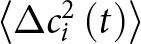 $\left\langle\Delta c_i^2\left(t\right)\right\rangle$ which did not meet a minimum travel distance of ≥1 particle radius (Fig. 3). The refined results yield consistent results in which
 $\left\langle\Delta c_i^2\left(t\right)\right\rangle$ increases with temperature and decreases with pressure. To calculate η (equation 2), we used only the
 $\left\langle\Delta c_i^2\left(t\right)\right\rangle$ which was consistently linear with time, that is, after it reaches a steady-state (Fig. 2). We estimate the uncertainty in our results is typically <16% at one standard deviation, which is consistent with previous work (Catipovic et al., Reference Catipovic, Tyler, Trapani and Carter2013) (Table 2).
We find clear and consistent trends in our viscosity results η values (Fig. 4). The positive temperature- and negative pressure-effects agree well with previous studies on water viscosity (Mukai et al., Reference Mukai, Deguchi and Tsujii2006; Abramson, Reference Abramson2007; Huber et al., Reference Huber, Perkins, Laesecke, Friend, Sengers, Assael, Metaxa, Vogel, Mareš and Miyagawa2009). Yet, while our results are internally consistent, we note our measured values are ∼4 to 9 times higher than predicted by the standard reference water viscosity given by the International Association for the Properties of Water and Steam (IAPWS) (Table 2; Fig. S1). Dissolution of the quartz particles into the water could significantly raise the fluid viscosity (Audétat and Keppler, Reference Audétat and Keppler2004). However, quartz solubility in water is also strongly temperature dependent. At room temperatures, only trace amounts of several parts per million (ppm) SiO2 dissolve in water (Morey et al., Reference Morey, Fournier and Rowe1962; Manning et al., Reference Manning1994; Makhluf et al., Reference Makhluf, Newton and Manning2023). In contrast, at least a thousand ppm of dissolved SiO2 may be needed to begin affecting the fluid viscosity significantly (Audétat and Keppler, Reference Audétat and Keppler2004). If the particle dissolution in our experiments is so extensive during heating, the fluid viscosity should increase with temperature as more quartz dissolves. Yet, this trend is not observed (Fig. 4).
The viscosity (η) of water as a function of pressure and temperature. Solid squares represent the results from this study. Small circles represent previous results which also used the Brownian motion method, but with polystyrene spheres (Mukai et al., Reference Mukai, Deguchi and Tsujii2006). Diamonds show constraints from rolling sphere experiments (Abramson, Reference Abramson2007). The solid lines and star represent the viscosity of water from the IAPWS reference (Huber et al., Reference Huber, Perkins, Laesecke, Friend, Sengers, Assael, Metaxa, Vogel, Mareš and Miyagawa2009). The lines are calculated using the reference IAPWS model with the approximate densities of H2O from our experiments (Table 1). All results are colour-coded by pressure.

Instead, we suspect that the higher measured viscosity is more likely to be due, at least in part, to undesirable drag effects acting on the particles due to the finite size of the sample chamber (Ashley et al., Reference Ashley, Mookherjee, Xu, Yu, Manthilake and Wang2024b). The main sources of drag are probably the gasket chamber walls and the diamond culets, meaning the bottom and top of the chamber (Fig. 1). In falling sphere experiments, drag due to the walls, known as the ‘wall effect’, is proportional to the sphere/particle-to-chamber diameters, i.e. d/D (Faxén, Reference Faxén1922). The tiny diameter of the particles compared to the gasket chamber diameter in our study results in d/D ≈ 0.005 which should yield negligible drag from the chamber walls (Brizard et al., Reference Brizard, Megharfi, Mahé and Verdier2005; Ashley et al., Reference Ashley, Mookherjee, Xu, Yu, Manthilake and Wang2024b). Previous Brownian motion experiments also found that the wall effect on the particles may be minimized when d/D ≤ 0.01 (Pigott et al., Reference Pigott2011). Our recording region also focused on the centre of the chamber to maximize the particle distance from the walls and further minimize any wall effect.
Many of the particles clearly settled over time to the bottom culet (Fig. 2; Videos S1, S2). The decreasing distance between the particles and diamond culet will increase the drag acting on the particles, often referred to as an ‘end effect’ (Ashley et al., Reference Ashley, Mookherjee, Xu, Yu, Manthilake and Wang2024b). The correction for such drag acting on the particles undergoing Brownian motion is described by
 \begin{equation}\unicode{x03B7}\left(z\right)=\unicode{x03B7}\cdot\left[1-\frac9{16}\left(\frac rz\right)\!+\frac18\left(\frac rz\right)^3\!\!-\frac{45}{256}\left(\frac rz\right)^4\!\!-\frac1{16}\left(\frac rz\right)^5\!\!+\dots\right]^{-1}\end{equation}
where η(z) represents the apparent viscosity as a function of distance z from the bottom culet (Fig. 1) and … represents higher order and negligible terms which are omitted (Goldman et al., Reference Goldman, Cox and Brenner1967; Feitosa and Mesquita, Reference Feitosa and Mesquita1991; Lin et al., Reference Lin, Yu and Rice2000). Terms at the 3rd and higher orders are also often omitted due to their negligible influence on η(z) (Pralle et al., Reference Pralle, Florin, Stelzer and Hörber1998; Dufresne et al., Reference Dufresne, Altman and Grier2001).
Notably, it is somewhat challenging to directly determine the z-distance of the particles. The Brownian motions are three-dimensional, hence the particles are likely to undergo random fluctuation in z-values between the bottom and top diamond culets. At a minimum, the particles must maintain a z-distance greater than their radius to avoid adhering to the culet, i.e. z ≥ r (Fig. 1). Further constraints on z may be made by comparing η(z) (equation 4) to our measurements.
While equation 4 does predict a dramatic increase in the apparent η with decreasing z (i.e. η(z)), it requires z < r (Fig. S1). These unrealistically small z-values suggest that equation 4 does not sufficiently describe the drag acting on the particles. We may also consider additional drag coming from the top culet, as in
 \begin{equation}{{\unicode{x03B7}}}\left( z \right) = {{\unicode{x03B7} }} \cdot {\left[ {1 - \frac{9}{{16}}\left( {\frac{r}{{{z_{btm}}}}} \right) - \frac{9}{{16}}\left( {\frac{r}{{{z_{top}}}}} \right)} \right]^{ - 1}}\end{equation}
where zbtm and zTop represent the distances from the bottom and top culets, respectively (Russel et al., Reference Russel, Saville and Schowalter1991) (Fig. 1). This function improves the agreement between η(z) with our measured values but again requires z < r (Fig. S1). We have also considered other corrections for η(z) (Dufresne et al., Reference Dufresne, Altman and Grier2001). Regardless of correction, we find that these functions require unrealistically small z-distances for the particles. This suggests that another source of drag must also be acting on the particles and increasing the measured viscosity.
We suspect that the additional drag needed to explain the high viscosities come from interactions among the particles themselves (Fig. 1). Two randomly vibrating spheres will influence the diffusivity relative to each other but also introduce a diffusivity for the centre-of-mass (Batchelor, Reference Batchelor1976; Crocker and Grier, Reference Crocker and Grier1996). As diffusivity (D) is directly related to MSD, and hence inversely related to viscosity (equation 2), these particle–particle interactions will also affect the viscosity measurements. Previous work (Batchelor, Reference Batchelor1976) considered expressions for the separate particle diffusivities and the combined centre-of-mass. The diffusivities relative to the centre-of-mass are given by:
 \begin{equation}D_{RM}^{{\parallel}} = \frac{{{D_0}}}{2}\left[ {1 - \frac{3}{2}\left( {\frac{r}{L}} \right){\text{ }} + {{\left( {\frac{r}{L}} \right)}^3} - \frac{{15}}{4}{{\left( {\frac{r}{L}} \right)}^4} + \ldots } \right]
\end{equation}
and
 \begin{equation}D_{RM}^ \bot = \frac{{{D_0}}}{2}\left[ {1 - \frac{3}{4}\left( {\frac{r}{L}} \right) - \frac{1}{2}{{\left( {\frac{r}{L}} \right)}^3} + \ldots } \right]\end{equation}
where  $D_{RM}^\parallel $ and
 $D_{RM}^ \bot $ represent the diffusivities along (||) the centre-centre line and perpendicular (⊥) to it, the subscript RM indicates relative to the centre-of-mass, and L is the length distance between the interacting particles (Fig. 1). The centre-of-mass diffusivity is described by:
 \begin{equation}D_{CM}^\parallel = \frac{{{D_0}}}{2}\left[ {1 + \frac{3}{2}\left( {\frac{r}{L}} \right) - {{\left( {\frac{r}{L}} \right)}^3} - \frac{{15}}{4}{{\left( {\frac{r}{L}} \right)}^4} + \ldots } \right]\end{equation}
and
 \begin{equation}D_{CM}^ \bot = \frac{{{D_0}}}{2}\left[ {1 + \frac{3}{4}\left( {\frac{r}{L}} \right) + \frac{1}{2}{{\left( {\frac{r}{L}} \right)}^3} + \ldots } \right]\end{equation}
where the subscript CM indicates the centre of mass.
Previous experiments showed that the DRM are suppressed by closing the gap between particles, whereas the DCM is enhanced (Crocker and Grier, Reference Crocker and Grier1996). The centre-of-mass motions are not tracked in TrackPy, hence the RM results are most applicable to our data. We would expect the suppressed diffusivity to also enhance the measured viscosity, which is consistent with our observations (Fig. S1). However, there is a challenge in precisely correcting this influence for these experiments. To ensure that our experiments contained enough suspended particles for tracking at high temperatures, it was necessary to provide significantly more particles than the two considered above. Although particle tracking software works quite well to identify the particles, significant care and testing is needed to filter false detections or non-robust movements, that is, particles which move in-and-out of focus or have short MSDs (Catipovic et al., Reference Catipovic, Tyler, Trapani and Carter2013; Allan et al., Reference Allan, Caswell, Keim, van der Wel and Verweiji2024). For a many-particle system as in this study (e.g. Fig. 2), filtering will ignore particles that still contribute to particle interactions. At the same time, poor filtering could introduce additional detections which may be false or increase the uncertainty of the measurements (Catipovic et al., Reference Catipovic, Tyler, Trapani and Carter2013; Allan et al., Reference Allan, Caswell, Keim, van der Wel and Verweiji2024). In the case of false detections, the particle–particle interactions may be over-estimated. Beyond this analytical challenge, the addition of more than two particles, as in this study, probably affects the particle–particle flow dynamics beyond that considered by equations 5 to 8. These inter-particle interactions may be further affected by variations in particle size or shape. Regardless, assuming that particle-pair-interactions are representative of our system, the interactions may increase the measured viscosity by a factor of two or three for nearby particles (Crocker and Grier, Reference Crocker and Grier1996). This effect could help explain the discrepancy in equations 4 and 5 with the high viscosities measured in our study (Fig. S1).
Based on the challenge to clearly account for the drag of a many-particle system, we chose to correct our results using the IAPWS reference model for the viscosity of water (Huber et al., Reference Huber, Perkins, Laesecke, Friend, Sengers, Assael, Metaxa, Vogel, Mareš and Miyagawa2009) (Fig. S1). To maintain the internal consistency of our dataset, we used only experiment 230908 to develop a correction for our results. The viscosity measured in this experiment is typically 4–9 times higher than predicted by the IAPWS reference at the same pressure, i.e. 0.3 GPa (Fig. S1). The ratio varies with temperature, which can be explained by the settling of particles and hence a decreasing z-distance. A similar trend was observed in previous Brownian motion experiments (Mukai et al., Reference Mukai, Deguchi and Tsujii2006). We find the ratio trend is well-described by an empirical exponential function given by
 \begin{equation}\frac{{{{{\unicode{x03B7}}}_{\text{M}}}}}{{{{{\unicode{x03B7} }}_{\text{C}}}}} = {\text{ }}{m_1}\exp \left( { - {m_2}T} \right) + {m_3}\end{equation}
where ηM and ηC are the measured and corrected viscosities, respectively, and serves as the correction coefficient, while the fit coefficients m 1, m 2 and m 3 are –7.6 ± 0.7, 0.016 ± 0.003 and 8.9 ± 0.4, respectively. While broadly empirical, equation 10 allows us to correct the results without assumption of the type(s) of drag acting on the particles.
Discussion
The viscosity results from our study compare broadly well with other constraints on the viscosity of water at high pressures ≥0.3 GPa (Fig. 4). However, the absolute values of viscosity from the Brownian motion tracking viscometry are significantly lower than those from rolling sphere measurements at higher pressures ≥1.6 GPa and temperatures >25°C (Fig. S2). We suspect the difference might be in part due to deformation of the DAC gaskets with heating, especially at high pressures. The change in gasket form would enhance boundary drag effects and require careful reconsideration for any drag corrections (King et al., Reference King, Herbolzheimer and Cook1992). However, no such deformation was reported in the previous rolling sphere experiments at >1.6 GPa (Abramson, Reference Abramson2007). Corrections for drag effects in the previous study (Abramson, Reference Abramson2007) were also not clearly documented or were assumed to be constant from earlier work (King et al., Reference King, Herbolzheimer and Cook1992; Abramson, Reference Abramson2005). It is therefore unclear if changing drag effects influenced the results of the previous study. Rotation resistance due to sphere roughness and the spacing length between the diamond culets might also be significant controls on the drag affecting rolling spheres (Eichler et al., Reference Eichler, Stefanski, Roca, Daniel, Issenmann, Valeriani and Caupin2025). In our present study, the small particle size relative to the DAC gasket walls (d/D < 0.01) should minimize the influence of changing drag effects from gasket deformation with heating. We also did not observe obvious gasket deformation in our experiments, due to the low P < 2.5 GPa and T ≤ 200°C. The drag effects observed in our experiments should then be largely independent of pressure. This suggests that the previous rolling sphere results at ≥1.6 GPa and >25°C may be overestimated.
We note an excellent agreement between our measured pressure-dependence, which is not affected by the drag correction (eq. 10), with that of the standard reference model for water (Huber et al., Reference Huber, Perkins, Laesecke, Friend, Sengers, Assael, Metaxa, Vogel, Mareš and Miyagawa2009) (Fig. 4). The pressure-dependence can be further evaluated by the activation volume (V ɑ) given by an Arrhenius function which describes our results, or
 \begin{equation}{{\unicode{x03B7}}} = {{{\unicode{x03B7} }}_0}.\exp \left( {\frac{{{E_a} + P{V_a}}}{{RT}}} \right)\end{equation}
where η0 is the pre-exponential viscosity term, P is pressure, R is the ideal gas constant, and T is absolute temperature, and E ɑ is the activation energy. Notably, there is also a nice agreement in the pressure-effects constrained by the rolling sphere and particle tracking methods, regardless of the disparity in viscosity values at high P ≥1.6 GPa (Table 3).
Comparison of Arrhenian function coefficients for various geofluids

Notes: The abbreviations HDAC, DAC, FPMD and MA refer to hydrothermal diamond-anvil-cell, diamond-anvil-cell, first-principles molecular dynamics (simulations) and multi-anvil, respectively.
The available constraints on the viscosities of various geofluids provide a first-order insight into their movement and roles within the Earth (Fig. 5). For instance, magmatism in subduction zones involves a wide range of geofluids from water-rich, aqueous fluids to aluminosilicate-rich melts (Grove et al., Reference Grove, Till and Krawczynski2012; Green et al., Reference Green, Hibberson, Rosenthal, Kovács, Yaxley, Falloon and Brink2014; Tatsumi et al., Reference Tatsumi1989; Ulmer Reference Ulmer2001; Stern, Reference Stern2002; Ducea et al., Reference Ducea, Saleeby and Bergantz2015). Erupting lavas along these convergent boundaries are typically aluminosilicate-rich melts produced from chemical evolution of more aluminosilicate-poor, parental magma (Stern, Reference Stern2002; Ducea et al., Reference Ducea, Saleeby and Bergantz2015). Such aluminosilicate-rich melt is often highly viscous (>103 Pa s) due to a highly polymerized network of silicon and aluminium (Si,Al) connected by ‘bridging’ oxygens, i.e. (Si,Al)–O–(Si,Al), which dominate the atomistic-scale melt structure and restrict movement of atoms (Richet, Reference Richet1984; Dingwell, Reference Dingwell1995) (Fig. 5). Increasing temperature helps to break some of the network linkages and thereby decrease the melt viscosity (Mysen, Reference Mysen1990; Stebbins and Xu, Reference Stebbins and Xu1997). Yet, addition of H2O to silicate melt may also break connections in the network by reacting with bridging oxygens to produce terminal hydroxyl units (Stolper, Reference Stolper1982; Hui et al., Reference Hui, Zhang, Xu and Behrens2008). The effect of adding several wt.% H2O to the melt may be comparable to increasing the temperature by a couple of hundred degrees (Ashley et al., Reference Ashley, Bajgain and Mookherjee2024a; Xie et al., Reference Xie, Andrault, Yoshino, Han, Hammond, Xu and Dobson2025). The silica-poor, parental magmatism is driven by hydrous melting of the mantle wedge, which is promoted by water-rich fluids ascending from the downgoing slab (Tatsumi et al., Reference Tatsumi1989; Grove et al., Reference Grove, Till and Krawczynski2012). Our results highlight that such water-rich fluids are likely to be highly mobile due to very low viscosities at even low temperatures (Fig. 5). Magmatic processes can therefore be strongly promoted by the addition of H2O.
(a) Schematic illustration of a subduction zone with potential geofluids and their migration paths. (b) The viscosity of water-rich fluids and aluminosilicate-rich melts as a function of pressure and temperature. Due to being very well-studied across a range of geofluid compositions from water- to silicate-rich, only albitic (NaAlSi3O8) compositions are shown for clear comparison. Solid and stippled lines indicate calculated viscosities from a modified Arrhenius model based on experiments and first-principles molecular dynamics (FPMD) simulations (Ashley et al., Reference Ashley, Mookherjee, Xu, Yu, Manthilake and Wang2025). Solid circles show experimental results on comparable supercritical fluids (Audétat and Keppler, Reference Audétat and Keppler2004). Hollow circles and dashed lines show results from FPMD simulations on aluminosilicate-rich, supercritical fluids (Long and Sun, Reference Long and Sun2025). Solid squares show results from this study (Table 2). Crosses (‘×’ and ‘+’) and hollow triangles show ambient temperature results from previous Brownian motion studies (Bowman et al., Reference Bowman, Gibson, Padgett, Saglimbeni and Di Leonardo2013; Frost and Glenzer, Reference Frost and Glenzer2020; Eichler et al., Reference Eichler, Stefanski, Roca, Daniel, Issenmann, Valeriani and Caupin2025). The dashed lines for pure H2O (this study) and supercritical fluids at 1727°C (Long and Sun, Reference Long and Sun2025) are calculated via the Arrhenian function (Table 3). For clarity, data or models from corresponding temperatures are highlighted by faded fields, and only a few temperature conditions from this study are shown. For supercritical fluids at ∼627 to 827°C (Audétat and Keppler, Reference Audétat and Keppler2004), data with comparable water contents are connected with faded lines. Abbreviations ‘aq.’ and ‘sc.’ indicate aqueous and supercritical, respectively.

We also note a dramatic change in the effect of pressure on the viscosities of geofluids (Fig. 5). The constraints on the viscosity of water display a positive pressure-dependence at P < 6 GPa (Table 3). Hence, water-rich fluids should become more mobile as they ascend and the viscosity decreases. The final aluminosilicate-rich melts in a subduction zone display an anomalous pressure-dependence in which viscosity first decreases and then increases with pressure, producing minima along isotherms (Fig. 5). The activation volume for silicate melt is typically negative at low pressures and becomes positive with compression (Table 3). This suggests that the melt may become less mobile as it ascends from sources at depth and could accumulate at depths relevant to the viscosity minima (Ashley et al., Reference Ashley, Bajgain and Mookherjee2024a, Reference Ashley, Mookherjee, Xu, Yu, Manthilake and Wang2025; Bajgain et al., Reference Bajgain, Peng, Mookherjee, Jing and Solomon2019; Bajgain and Mookherjee, Reference Bajgain and Mookherjee2020, Reference Bajgain and Mookherjee2021; Long and Sun, Reference Long and Sun2025; Sakamaki et al., Reference Sakamaki, Suzuki, Ohtani, Terasaki, Urakawa, Katayama, Funakoshi, Wang, Hernlund and Ballmer2013). The anomalous pressure-dependence has been explained by complex changes in the polymerized network of the melt, including collapsing (Si,Al)–O–(Si,Al) bond angles, breaking of network linkages, increasing coordination numbers of O around (Si, Al), compaction of atoms to a critical packing limit, and formation of new connections at high pressures (Allwardt et al., Reference Allwardt, Poe and Stebbins2005a, Reference Allwardt, Stebbins, Schmidt, Frost, Withers and Hirschmann2005b; Allwardt et al., Reference Allwardt, Stebbins, Terasaki, Du, Frost, Withers, Hirschmann, Suzuki and Ohtani2007; Kelsey et al., Reference Kelsey, Stebbins, Mosenfelder and Asimow2009; Malfait et al., Reference Malfait, Verel, Ardia and Sanchez-Valle2012; Wang et al., Reference Wang, Sakamaki, Skinner, Jing, Yu, Kono and Sutton2014). Supercritical fluids, which could serve as effective transport agents in appropriate conditions in subduction zones, might be both water- and silicate-rich (Shen and Keppler, Reference Shen and Keppler1997; Bureau and Keppler, Reference Bureau and Keppler1999; Kessel et al., Reference Kessel, Ulmer, Pettke, Schmidt and Thompson2005a, Reference Kessel, Schmidt, Ulmer and Pettke2005b; Audétat and Keppler, Reference Audétat and Keppler2004). We note that such fluids with 30 to 50 wt.% H2O may display a weak but positive linear pressure-dependence (Long and Sun, Reference Long and Sun2025) (Table 3; Fig. 5). This suggests that the supercritical fluid structure is already mostly depolymerized and comparable to pure water at these H2O contents. Furthermore, the mobility of such supercritical fluids should not be significantly influenced by depth-induced changes to the viscosity. However, fluids with lower water contents could display a more melt-like viscosity trend and hence an anomalous pressure-dependence (Fig. 5). This may occur as the supercritical fluids ascend, potentially react with the mantle, and ultimately destabilize as they approach conditions relevant to partial melting of the mantle wedge in a subduction zone.
Conclusions
Our results indicate that the Brownian motion method has potential for investigating the viscosities of fluids at high-pressure, hydrothermal to supercritical conditions. Our experiments show that small quartz grains in water can display measurable Brownian motions even at high temperatures. This study highlights the potential to use materials which are more chemically resistant/refractory than plastics such as polystyrene, but also relatively more dense. However, there are still obstacles in exploring high temperatures due to the negative buoyancy of such denser materials. The enhanced settling with heating, due to decreasing fluid viscosity, effectively removes particles to track. Modifications to a DAC, such as recessed cavities (Saha et al., Reference Saha, Anderson, Lee and Klemm2017), could perhaps allow targeted release of the particles similar to the trap method in falling sphere experiments (Terasaki et al., Reference Terasaki, Kato, Urakawa, Funakoshi, Suzuki, Okada and Kasai2001, Reference Terasaki, Suzuki, Ohtani, Nishida, Sakamaki and Funakoshi2006; Liebske et al., Reference Liebske, Schmickler, Terasaki, Poe, Suzuki, Funakoshi, Ando and Rubie2005). Yet, a substantial number of particles may still be needed to ensure a usable suspension. The higher particle concentration will probably increase drag effects from particle–particle interactions. Updates to particle tracking codes may help to quantify such interactions, but this may also become more challenging with increasing particle density. Until these challenges are overcome, the Brownian motion method may still be limited in exploring novel systems. Alternative viscometry methods, such as the falling sphere method or finite element modelling of induced convection currents (Bartlett et al., Reference Bartlett, Gomez-Perez, Hermes and McWilliams2020), will provide helpful comparisons. These complementary methods will help to further identify the movement and transport roles of various geofluids at conditions relevant to the interior of Earth and other planets.
Supplementary material
The supplementary material for this article can be found at https://doi.org/10.1180/mgm.2026.10195.
Acknowledgements
We thank two anonymous reviewers and the editor, Roger Mitchell, for their constructive feedback and careful handling of our manuscript.
Funding statement
A.W. A. acknowledges the Buie, DeVore, and Watkins Fund from the Department of Earth, Ocean and Atmospheric Sciences, Florida State University. M.M. acknowledges the National Science Foundation grant (EAR-2246802) for funding this research. The experiments were performed at Florida State University within the Earth Materials Lab.
Competing interests
The authors declare none.



