I. INTRODUCTION
In wireless communication, it is necessary to boost the power of the transmitted signal to such a level that the signal is not masked by the noise and interference when it reaches the intended receiver. The necessary amplification is handled by the radio frequency (RF) power amplifier (PA). However, RF PAs tend to have either low distortions and low-power efficiency (a small fraction of consumed power is converted into useful RF signal), or large distortions and high-power efficiency [Reference Cripps1].
The distortions introduced by the RF PA are dynamic and nonlinear. The linear dynamic distortions, also known as linear frequency dependency or linear memory effects, introduce errors in the transmitted signal within the band. These errors degrade the performance of the communication system in the form of increased bit error rate (BER) at the intended receiver. The nonlinear distortions, which typically also are dynamic, also decrease the performance of the communication system by distorting the transmitted signal within the band [Reference Schreurs, O'Droma, Goacher and Gadringer2, Reference Cripps3]. However, nonlinear distortions do also cause spectral regrowth, i.e. a spectral spreading of the input signal. This spectral spreading means that energy is leaking into adjacent channels, possibly interfering with other transmitter–receiver pairs operating in that frequency range. In order to limit these effects, regulatory bodies have put limitations on the amount of allowed power leaking into adjacent channels or requirements of passing a spectral mask. Two examples are the limits on adjacent channel leakage power ratio (ACLR) specified by 3rd Generation Partnership Project (3GPP) [4, 5].
In order to reduce the distortions, linear PAs can be used at the cost of significant loss of power efficiency which is not acceptable. Therefore, one method is to design a nonlinear and power efficient PA and then apply a correction technique to reduce the distortions. In this way a linearly behaving and power efficient transmitter is achievable. The linearization can be implemented using a number of techniques. Among these are feedforward, feedback, predistortion, and linear amplification using nonlinear components (LINC), to mention a few [Reference Vuolevi and Rahkonen6].
One popular method is through digital pre-distortion (DPD), i.e. to place an inverse of the PA distortions in front of the PA such that this inverse cancels the distortions generated by the PA. When designing the inverse it is first necessary to know how the distortions are affecting the signal, i.e. the direct model of the PA should be known such that the inverse of the distortions can be computed. However, it also turns out that under the assumption of negligible linear frequency dependency, the inverse model has the same form, considered as Volterra kernels, as the direct model [Reference Isaksson and Rönnow7]. This is commonly used in DPD by utilizing the same model structure for direct modeling as for linearization, see [Reference Isaksson and Rönnow7–Reference Ghannouchi and Hammi11] for a few examples.
Memory polynomial (MP) models appear to have become the de facto standard for RF PA modeling [Reference Landin, Isaksson and Händel12]. One of the most commonly used MP models is the parallel Hammerstein (PH) [Reference Kim and Konstantinou8, Reference Heutmaker, Wu and Welch13]. Another commonly used model structure is the generalized memory polynomial (GMP) proposed in [Reference Morgan, Ma, Kim, Zierdt and Pastalan14]. Other MP models have also been proposed, but most of them appear to have been constructed in a, more or less, ad hoc manner. The performance of the models have then verified by measurements of different PA in labs throughout the world. Not until recently has physical motivations for some of these models been given by [Reference Cunha, Lima and Pedro15].
In this paper, we propose to start from general physical knowledge of a RF PA and use this to derive two novel MP model structures. The derivations and necessary assumptions are given so that it is possible to derive other model structures, if desired.
The performance of the derived models is tested using measured data from two RF amplifiers, one high-power PA and one general purpose low-PA. The model error of the two novel model structures is shown to be lower than for previously proposed model structures given a certain number of parameters. A relation between one of the derived models and the third-order Volterra kernel of the tested PA is also shown.
The background and the derivations are given in Section II. Experimental setup is described in Section III and results together with the discussion in Section IV. Conclusions are then drawn in Section V.
II. THEORY
This section introduces the background knowledge in the form of the nonlinear feedback system from [Reference Pedro, Carvalho and Lavrador16] and derives the two novel MP models, given certain properties of the RF PA.
The information-carrying signal in most wireless communication signal is a so-called (real-valued) band-pass signal [Reference Proakis17], i.e. it is a narrowband modulated signal centered at a high-frequency carrier. Typical examples are telecommunication signals with bandwidths of 5 MHz and carrier frequencies of several GHz as in the universal mobile telecommunications system (UMTS). However, because the only behavior of interest is that close to the carrier a more commonly used representation is the (possibly complex-valued) equivalent lowpass [Reference Proakis17]. In this section, all equivalent low-pass signals use the subscript LP, i.e. x LP(t),y LP(t) whereas the corresponding band-pass signals are x(t),y(t).
The relation between lowpass and bandpass can be expressed as [Reference Proakis17]
 $$\eqalign{x\lpar t\rpar &= \alpha \lpar t\rpar \cos \lpar \omega_c t + \phi \lpar t\rpar \rpar = \Re \left\{\alpha \lpar t\rpar e^{j\varphi \lpar t\rpar } e^{j\omega_{c} t} \right\}\cr &= \Re \left\{x_{LP} \lpar t\rpar e^{j \omega_{c} t} \right\}\comma \; }$$
where α(t) is the amplitude modulation, ϕ(t) is the phase modulation and ω c is the carrier frequency. ℜ{·} denotes the real part of a complex number. We assume that the input signal x(t) to a PA is narrowband, i.e. that the modulation bandwidth is narrow compared to the carrier frequency. This means that the signal spectrum centered at one harmonic does not overlap with the spectrum from another harmonic.
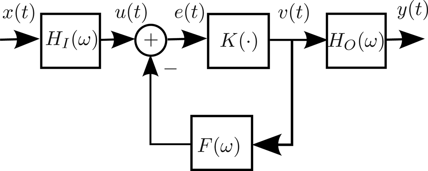
The physical knowledge about the PA behavior comes from a nonlinear circuit representation in [Reference Pedro, Carvalho and Lavrador16] transformed to a nonlinear feedback system [Reference Pedro, Carvalho and Lavrador16] shown in Fig. 1. The passive input and output matching networks are represented by dynamic linear band-pass filters H I(ω) and H O(ω) centered at the carrier frequency. The feedback filter F(ω) is a low-pass filter representing low-frequency or “long-term memory” such as thermal memory and bias modulation [Reference Pedro and Maas18]. The frequency regions of the three linear filters are illustrated in Fig. 2.
The model structure proposed in [Reference Pedro, Carvalho and Lavrador16], which represents the band-pass behavior of a RF PA. H I(ω) and H O(ω) are linear filters representing the input and output matching networks, F(ω) is a linear filter for the feedback representing bias modulation and thermal memory effects, and K(·) is a static nonlinearity [Reference Pedro and Maas18]. x(t) is the input voltage, and y(t) is the output voltage.

Illustration of the filter behavior with the input and output signals from the static nonlinearity K(·). The low-pass filter F(ω) removes all signal components above a given frequency, which is here illustrated as retaining the spectral components close to DC. The filters H I(ω) and H O(ω) are band-pass filters that pass the frequency components close to the carrier.
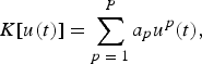
The block K(·) is the nonlinear current source generating the nonlinear distortion. This nonlinearity mainly depends on the class of operation, i.e. A, AB, B etc. It is assumed that the static nonlinearity K(·) can be represented by the polynomial
 $$K\lsqb u\lpar t\rpar \rsqb = \sum\limits_{p \;=\; 1}^P a_p u^p \lpar t\rpar \comma \;$$
where a p are the polynomial coefficients. For simplicity we also assume that P is odd. We can equally well use an even P; the only change would be the upper summation limits. Note that the model in Fig. 1 is used as a model at a given operating point, i.e. a 0 is 0.
Using the assumption of a polynomial static nonlinearity makes it impossible to derive terms involving x(n)|x(n)|2p−1, where p is a positive integer. However, in [Reference Landin and Rönnow19] it was shown that these “even” terms only induce a difference in the truncation error already present in the models due to finite nonlinear order, i.e. the model representations are identical up to the truncation error of order  ${\cal O}\lpar P+2\rpar $, where P is the odd model order. However, it should be noted that these “even” terms also have a physical meaning for systems that have two (or more) inputs. In [Reference Stauth and Sanders20], it was discussed how the supply voltage ripple is mixed onto the carrier through the multiplication between the low-frequency ripple and the carrier signal in the even order nonlinearities. Thus, the ripple appears in the high-frequency band-pass region. The results in [Reference Cunha, Lima and Pedro15] can be interpreted in a similar fashion, namely that there is a second input signal that also affects the nonlinear behavior in the pass-band region.
We assume that the frequency dependency of the input matching network is negligible so that the signal u(t) is only a delayed and linearly scaled version of x(t), i.e.
 $$u\lpar t\rpar = h_I x\lpar t - \delta_I\rpar \comma \;$$
where h I is the amplitude scaling and δ I is the delay. This is reasonable as a strong frequency dependency would degrade the error vector magnitude (EVM) of an amplified signal considerably. Without this assumption the resulting system would be a Wiener-type system, i.e. a dynamic linear block followed by a static nonlinearity. If a PA would present significant memory effects in the input matching network, Hammerstein and MP approaches would result in large model errors, which is not normally the case.
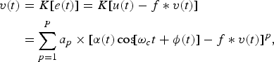
The output of the static nonlinearity can then be expressed as
 $$\eqalign{v\lpar t\rpar &= K\lsqb e\lpar t\rpar \rsqb = K\lsqb u\lpar t\rpar - f \ast v\lpar t\rpar \rsqb \cr & = \sum\limits_{p = 1}^P a_p \times \lsqb \alpha \lpar t\rpar \cos \!\lsqb \omega_c t + \phi \lpar t\rpar \rsqb - f \ast v\lpar t\rpar \rsqb ^p\comma \; }$$
where α(t) and ϕ(t) are the amplitude and phase modulation, respectively. Here, f is the impulse response of the feedback filter F(ω).
v(t) is really the result of an infinite sum of loops in the feedback path. However, for practical MP models it is assumed that both the nonlinear order P and the memory depth is finite. Thus, it is assumed that the feedback can be broken to get the signal v 1(t) which denotes the output from K(·) after one loop in the feedback path:
 $${v_1}\lpar t\rpar = \sum\limits_{p=1}^P a_p \lcub \alpha \lpar t\rpar \cos \!\lsqb \omega t + \phi \lpar t\rpar \rsqb - f \ast v\lpar t\rpar \rcub ^p + {\cal O} \lpar \lsqb f \ast v\lpar t\rpar \rsqb ^2\rpar .$$
The notation  ${\cal O}\lpar{\cdot}\rpar $ denotes the Ordo-notation [Reference Adams21] which tracks the largest order of the truncation error. In this case the truncation errors are on the order of [f*v(t)]2.
Maintaining the feedback leads to a kind of repeated Wiener structure because the filtering of v(t) by F(ω) followed by the static nonlinearity K(·) is indefinitely repeated in the feedback loop. This repetition results in a signal v(t) of infinite nonlinear order and infinite memory. Breaking the feedback loop is discussed in [Reference Pedro and Maas18, Reference Wisell and Isaksson22–Reference Cunha, Pedro and Cabral25].
If the filter F(ω) is assumed to be a low-pass filter, it is possible to split v(t) into two components
 $${v_1}\lpar t\rpar = v_{DC} \lpar t\rpar + v_{CC} \lpar t\rpar + {\cal O} \lpar \lsqb f \ast v\lpar t\rpar \rsqb ^2\rpar \comma \;$$
such that
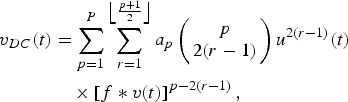 $$\eqalign{v_{DC} \lpar t\rpar &= \sum\limits_{p = 1}^P \sum\limits_{r = 1}^{\left\lfloor {p + 1 \over 2} \right\rfloor} a_p \left(\matrix{p \cr 2\lpar r - 1\rpar } \right)u^{2\lpar r - 1\rpar } \lpar t\rpar \cr &\quad \times \left[f \ast v\lpar t\rpar \right]^{p - 2\lpar r - 1\rpar }\comma \; }$$
has spectral components close to DC and
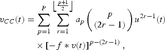 $$\eqalign{v_{CC} \lpar t\rpar &= \sum\limits_{p = 1}^P \sum\limits_{r = 1}^{\left\lfloor{p + 1 \over 2} \right\rfloor} a_p \left(\matrix{p \cr \lpar 2r - 1\rpar } \right)u^{2r - 1} \lpar t\rpar \cr &\quad \times \left[- f \ast v\lpar t\rpar \right]^{p - \lpar 2r - 1\rpar }\comma \; }$$
has spectral components close to the carrier. If the feedback filter F(ω) is also allowed to pass signal components at the fundamental and second harmonic the resulting model becomes more complex, as shown in the Appendix.
F(ω) is assumed to be of low-pass character which means that only the signal components close to DC are kept. Thus, the signal components that are output from F(ω) contain even orders of u(t). Furthermore, because the feedback is broken after one round, there is no additional filtering taking place, i.e. the output signal is given by
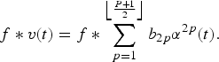 $$f \ast{v} \lpar t\rpar = f \ast \sum\limits_{p = 1}^{\left\lfloor {P + 1 \over 2} \right\rfloor} b_{2p} \alpha^{2p} \lpar t\rpar .$$
The coefficients b 2p = a 2p/2p are scaled versions of the a 2p-coefficients. This scaling comes from considering  $a_{2p} u^{2p} \lpar t\rpar = a_{2p} \left\{\alpha^2 \lpar t\rpar /2\left[1 + \cos \lpar 2 \omega_c t\rpar \right]\right\}^p$ and comparing with (9).
The signal components close to the carrier should now be found. Only odd powers of u(t) can be present. Even powers are located either at DC or at the even harmonics. However, a common form of MP models also uses the so called “even order” terms  $x_{LP} \lpar t\rpar \vert x_{LP} \lpar t\rpar \vert^{\lpar 2p - 1\rpar }$, where p is an integer, in addition to the standard odd terms x LP(t)|x LP(t)|2(p−1). These “even order” terms cannot explicitly be derived using the assumptions in this paper. However, in [Reference Landin and Rönnow19], it was shown that the representations using “even order” terms is nothing but a change of basis compared to the standard odd order terms, up to a truncation error that is of the same order as the model truncation. Thus, in terms of descriptive performance there is no essential difference between odd and “even” order MP terms.
The signal components close to the carrier can then be expressed as
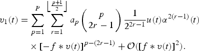 $$\eqalign{v_1 \lpar t\rpar &= \sum\limits_{p = 1}^P \sum\limits_{r = 1}^{\left\lfloor {p + 1 \over 2} \right\rfloor} a_p \left(\matrix{ p \cr 2r - 1} \right){1 \over 2^{2r - 1}} u\lpar t\rpar \alpha^{2\lpar r - 1\rpar } \lpar t\rpar \cr &\quad \times \left[- f \ast v\lpar t\rpar \right]^{p - \lpar 2r - 1\rpar } + {\cal O}\lpar \lsqb f \ast v\lpar t\rpar \rsqb ^2\rpar .}$$
This result follows from using the broken feedback of (9) in (5).
Two models are derived in the following starting from (10). We present them in separate sub sections in the following.
Before continuing, some notation related to bandwidth and sampling of the continuous time signals is introduced. The low-pass equivalent MP models are sampled in time at a sampling rate of T s. The low-pass equivalent signal sampled at time instance nT s is denoted by x LP(n). To avoid confusion the following definition of relevant bandwidth is introduced: By the relevant bandwidth of a signal, we mean a closed neighborhood around DC for low-pass equivalent signals and around the carrier for band-pass signals.
A) Model 1: EEMP
The first, to the knowledge of the authors, novel model is an extension of the envelope memory polynomial (EMP) proposed in [Reference Hammi, Ghannouchi and Vassilakis10, Reference Ghannouchi and Hammi11]. The EMP model lacks linear memory terms, making it less suitable for describing systems where there is a linear frequency dependency.
To derive the extended envelope memory polynomial (EEMP), we assume that the only significant mixing between the feedback term and the input signal is given by the second-order nonlinearity in K(·) as
 $$u\lpar t\rpar \lsqb - f \ast v\lpar t\rpar \rsqb .$$
Mixing of higher orders of the feedback signal −f*v(t) and odd harmonics of u(t) are assumed to be negligible. However, terms containing the static nonlinear behavior from K(·) are still included. In other words, the terms from (10) that are relevant fulfill either r = 1, p − (2r − 1) = 1 or p − (2r − 1) = 0 irrespectively of r.
These reductions lead to rewriting (10) as
 $$v_1 \lpar t\rpar = \sum\limits_{p = 1}^{\left\lfloor {P + 1 \over 2} \right\rfloor + 1} \hat{a}_{2p - 1} u\lpar t\rpar \hat{f} \ast \alpha^{2\lpar p - 1\rpar } \lpar t\rpar + {\cal O} \lpar \lsqb f \ast v\lpar t\rpar \rsqb ^2\rpar \comma \;$$
with  $\hat{a}_{2p - 1} = a_{2p - 1} - {a_1 \over 2} b_{2\lpar p - 1\rpar }$,
 $\hat{a}_{2\left(\left\lfloor {P + 1 \over 2} \right\rfloor + 1 \right)- 1} = - {a_1 \over 2} b_{2 \left\lfloor {P + 1 \over 2} \right\rfloor}$, and
 $\hat{f} = 1 - f$. Details of the derivation are provided in [Reference Landin, Barbé, Van Moer, Isaksson and Händel26].
Filtering v 1(t) from (12) by the output filter H O(ω) results in
 $$y\lpar t\rpar = \sum\limits_{p = 1}^{\left\lfloor {P + 1 \over 2} \right\rfloor + 1} \hat{a}_{2p - 1} h_O \ast \left\{u\lpar t\rpar \hat{f} \ast \alpha ^{2\lpar p - 1\rpar } \lpar t\rpar \right\}.$$
Converting (13) to baseband would result in a model similar to the GMP. However, the interest is not in the GMP model. Instead, using two additional assumptions, one related to the relative power of the linear and nonlinear signal components and the other to the frequency dependency of H O(ω) and F(ω), a model with reduced parameter-complexity can be found.
The first assumption states that the power of the linear signal component is significantly larger than the power of the nonlinear signal components in (13). This is a reasonable assumption as the PA is assumed to be weakly nonlinear.
The second assumption means that the frequency dependency of H O(ω) is considerably smaller than the frequency dependency of F(ω), within their relevant bandwidths. Frequency dependency here means any deviation from constant gain and linear phase. The exact definitions are clarified in [Reference Landin, Barbé, Van Moer, Isaksson and Händel26].
These two assumptions together means that the linear filtering by H O(ω) affects the linear term of (13) but can be ignored for the nonlinear signal components. This results in
 $$y\lpar t\rpar = a_1 h_O \ast u\lpar t\rpar + \sum\limits_{p = 2}^{\left\lfloor {P + 1 \over 2} \right\rfloor + 1} \hat{a}_{2p - 1} u\lpar t\rpar \hat{f} \ast \alpha^{2\lpar p - 1\rpar } \lpar t\rpar .$$
The above assumptions might seem controversial at first. However, the difference in signal power between linear and nonlinear components is significant. Thus, the total model error incurred by these assumptions is negligible when viewed as a total model error, e.g. the normalized mean square error (NMSE). However, it does not hold for the adjacent channel error power ratio (ACEPR), which focuses on the nonlinear signal components that are affected by the filtering.
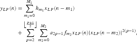
Transforming (14) to baseband and sampling results in
 $$\eqalign{y_{LP} \lpar n\rpar &= \sum\limits_{m_1 = 0}^{M_1} h_{m_1} x_{LP} \lpar n - m_1\rpar \cr&+ \sum\limits_{p = 2}^{\left\lfloor {P + 1 \over 2} \right\rfloor} \sum\limits_{m_2 = 0}^{M_2} a_{2p - 1} f_{m_2} x_{LP} \lpar n\rpar \vert x_{LP} \lpar n - m_2\rpar \vert^{2\lpar p - 1\rpar }\comma \;}$$
where h and f are the resulting impulse responses. However, (15) is nonlinear in the parameters a 2p−1 and  $g_{m_2}$. By applying a “parallelization”, i.e. allowing the filters to vary independently between the nonlinear orders, the EEMP model is found as
 $$\eqalign{y_{LP} \lpar n\rpar &= \sum\limits_{m_1 = 0}^{M_1} h_{m_1} x_{LP} \lpar n - m_1\rpar \cr&+ \sum\limits_{p = 2}^{\left\lfloor {P + 1 \over 2} \right\rfloor} \sum\limits_{m_2 = 0}^{M_2} g_{2p - 1\comma m_2} x_{LP} \lpar n\rpar \vert x_{LP} \lpar n - m_2\rpar \vert^{2\lpar p - 1\rpar }\comma} \;$$
where  $h_{m_1}$ and
 $g_{2p - 1\comma m_2}$ are the model parameters that are to be identified. Note that this operation is only done to provide an estimation problem that is linear in the parameters. The “parallelization” of filters is the same that transforms a Hammerstein structure into a PH, as shown in [Reference Söderström and Stoica27]. This parallelization brings the disadvantage of significantly increased parameter count.
The EEMP is a model that to the knowledge of the authors is a novel model structure for RF PA behavioral modeling.
B) Model 2: MNOMP
The mixed nonlinear order memory polynomial (MNOMP) model is a, to the knowledge of the authors, novel model structure that puts less restrictive assumptions on the mixing between the feedback signal components and the input signal in (10). Discarding all terms that do not fulfill either of
 $$p + \lpar 2r - 1\rpar = 0\comma \;$$
 $$p + \lpar 2r - 1\rpar = 1\comma \;$$
in (10), the result is
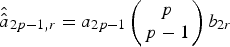
 $$v_1 \lpar t\rpar = \sum\limits_{p \;=\; 1}^{\left\lfloor {P + 1 \over 2} \right\rfloor} \sum\limits_{r \;=\; 1}^{\left\lfloor {P + 1 \over 2} \right\rfloor} \hat{\hat{a}}_{2p - 1\comma r} u\lpar t\rpar \alpha^{2\lpar p - 1\rpar } \lpar t\rpar \hat{f} \ast \alpha^{2r} \lpar t\rpar \comma \;$$
where  $\hat{\hat{a}}_{2p - 1\comma 0} = a_{2p - 1} \left(\matrix{p \cr p - 2} \right)- b_0 a_{2p - 1} \left(\matrix{p \cr p - 1} \right)$,
 $\hat{\hat{a}}_{2p - 1\comma r} = a_{2p - 1} \left(\matrix{p \cr p - 1} \right)b_{2r}$ if r ≥ 1 and
 $\hat{f} = 1 - f$.
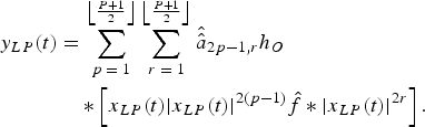
Apply the filter H O(ω) to (18) and convert to baseband to get
 $$\eqalign{y_{LP} \lpar t\rpar &= \sum\limits_{p \;=\; 1}^{\left\lfloor {P + 1 \over 2} \right\rfloor} \sum\limits_{r \;=\; 1}^{\left\lfloor {P + 1 \over 2} \right\rfloor} \hat{\hat{a}}_{2p - 1\comma r} h_O \cr &\quad \ast \left[x_{LP} \lpar t\rpar \vert x_{LP} \lpar t\rpar \vert^{2\lpar p - 1\rpar } \hat{f} \ast \vert x_{LP} \lpar t\rpar \vert^{2r} \right].}$$
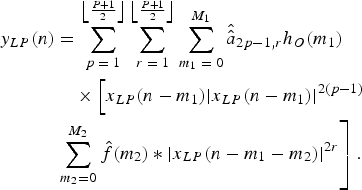
Sampling (19) results in
 $$\eqalign{y_{LP} \lpar n\rpar &= \sum\limits_{p \;=\; 1}^{\left\lfloor {P + 1 \over 2} \right\rfloor} \sum\limits_{r \;=\; 1}^{\left\lfloor {P + 1 \over 2} \right\rfloor} \sum\limits_{m_1 \;=\; 0}^{M_1} \hat{\hat{a}}_{2p - 1\comma r} h_O \lpar m_1\rpar \cr &\quad \times \left[x_{LP} \lpar n - m_1\rpar \vert x_{LP} \lpar n - m_1\rpar \vert^{2\lpar p - 1\rpar } \right. \cr & \left. \sum\limits_{m_2 = 0}^{M_2} \hat{f}\lpar m_2\rpar \ast \vert x_{LP} \lpar n - m_1 - m_2\rpar \vert^{2r} \right].}$$
If the filters h O(m 1) and  $\hat{f}\lpar m_2\rpar $ are considered to be independent of nonlinear order, i.e. parallelizing the filters [Reference Söderström and Stoica27] as was done for the EEMP, (20) results in
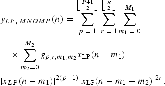 $$\eqalign{&y_{LP\comma \; MNOMP} \lpar n\rpar = \sum\limits_{p \;=\; 1}^{\left\lfloor {P + 1 \over 2} \right\rfloor} \sum\limits_{r \;=\; 1}^{\left\lfloor {R \over 2} \right\rfloor} \sum\limits_{m_1 \;=\; 0}^{M_1} \cr &\quad \times \sum\limits_{m_2 = 0}^{M_2} g_{p\comma r\comma m_1\comma m_2} x_{\rm LP} \lpar n - m_1\rpar \cr & \vert x_{LP} \lpar n - m_1\rpar \vert^{2\lpar p - 1\rpar } \vert x_{\rm LP} \lpar n - m_1 - m_2\rpar \vert^{2r}.}$$
Note that the upper summation limit over r has been given additional freedom compared to (20) by allowing R to vary independently of P. This is reasonable as the relative size of the feedback terms is not known. Thus, in order to have efficient parameterizations it is necessary to allow R to vary independently. The coefficients of the MNOMP model  $g_{p\comma r\comma m_1\comma m_2}$ are to be determined using suitable identification methods.
Note that the MNOMP is a superset of commonly used model structures. The MNOMP results in the following special cases if the nonlinear orders and/or memory depths are restricted:
• PH, if R = 1
• GMP, if P = 1
• EMP, if P = 1 and M 1 = 0.
C) Review of memory polynomials
As mentioned in the introduction, a large number of MP models have been proposed in the literature. The most commonly used of these models are here introduced for purposes of comparison with the models derived in the previous section.
The model structures considered here are only allowed to use the odd order representation [Reference Ding and Zhou28, Reference Ding and Zhou29], i.e. terms containing x LP(n)|x LP(n)|2(p−1) and no “even” order terms x LP(n)|x LP(n)|2p−1. It was in [Reference Landin and Rönnow19] shown that these two representations are equivalent up to the nonlinear order of the model.
The PH was introduced in [Reference Kim and Konstantinou8, Reference Heutmaker, Wu and Welch13] as
 $$\eqalign{y_{LP\comma PH} \lpar n\rpar = \sum\limits_{p \;=\; 1}^P \sum\limits_{m \;=\; 0}^M b_{p\comma m} x_{LP} \lpar n - m\rpar \vert x_{LP} \lpar n - m\rpar \vert^{2\lpar p - 1\rpar }\comma} \;$$
with coefficients b p,m, nonlinear order 2P−1 and memory depth M.
The GMP was proposed in [Reference Morgan, Ma, Kim, Zierdt and Pastalan14] as
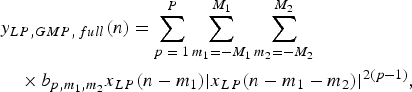 $$\eqalign{&y_{LP\comma GMP\comma \,full} \lpar n\rpar = \sum\limits_{p \;=\; 1}^P \sum\limits_{m_1 = - M_1}^{M_1} \sum\limits_{m_2 = - M_2}^{M_2} \cr &\quad \times b_{p\comma m_1\comma m_2} x_{LP} \lpar n - m_1\rpar \vert x_{LP} \lpar n - m_1 - m_2\rpar \vert^{2\lpar p - 1\rpar }\comma \; }$$
with coefficient  $b_{p\comma m_1\comma m_2}$, nonlinear order 2P−1 and memory depths M 1 and M 2. The original publication [Reference Morgan, Ma, Kim, Zierdt and Pastalan14] also allowed even order terms but we have chosen not to include these.
A common reduced version of (23) is obtained by removing the negative time-indexes to get
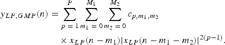 $$\eqalign{y_{LP\comma GMP} \lpar n\rpar &= \sum\limits_{p \;=\; 1}^P \sum\limits_{m_1 \;=\; 0}^{M_1} \sum\limits_{m_2 \;=\; 0}^{M_2} c_{p\comma m_1\comma m_2} \cr &\quad \times x_{LP} \lpar n - m_1\rpar \vert x_{LP} \lpar n - m_1 - m_2\rpar \vert^{2\lpar p - 1\rpar }.}$$
The number of parameters,  $c_{p\comma m_1\comma m_2}$ is significantly reduced for a given memory depth and nonlinear order compared to (23).
The extended parallel Hammerstein (EPH) model was proposed in [Reference Wisell and Isaksson22] based on the same feedback system as was used in this paper. The EPH is given by
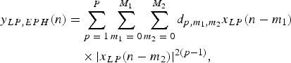 $$\eqalign{y_{LP\comma EPH} \lpar n\rpar &= \sum\limits_{p \;=\; 1}^P \sum\limits_{m_1 \;=\; 0}^{M_1} \sum\limits_{m_2 \;=\; 0}^{M_2} d_{p\comma m_1\comma m_2} x_{LP} \lpar n - m_1\rpar \cr &\quad \times \vert x_{LP} \lpar n - m_2\rpar \vert^{2\lpar p - 1\rpar }\comma \; }$$
with parameters  $d_{p\comma m_1\comma m_2}$ and memory depths and nonlinear order as earlier.
The EMP model was first given in [Reference Hammi, Ghannouchi and Vassilakis10, Reference Ghannouchi and Hammi11] as
 $$y_{LP\comma EMP} \lpar n\rpar = \sum\limits_{p \;=\; 1}^P \sum\limits_{m \;=\; 0}^{M_1} h_{p\comma m} x_{LP} \lpar n\rpar \vert x_{LP} \lpar n - m\rpar \vert^{2\lpar p - 1\rpar }\comma \;$$
with parameters h p,m.
With these commonly used behavioral models, we will compare the model performance using data from a class-AB RF PA.
III. MEASUREMENT SETUP
The performances of the previously derived models are to be compared using data measured on two commercially available RF amplifiers. One is a class-AB triple-stage PA from Ericsson AB. It had 52 dB small-signal gain and a rated 1 dB compression point output power of 53 dBm. The PA operated in the 2110–2170 MHz band and was intended as a multi-carrier PA in the UMTS using WCDMA-signals and feedforward linearization. The feedforward linearization was disabled during the tests.
The other amplifier was a Mini-Circuits ZVE-8G general purpose wideband linear amplifier. It had a nominal small-signal gain of 30 dB and output 1 dB compression point of 30 dBm. The used center frequency was 2.15 GHz.
The used test signals were of wideband code division multiple access (WCDMA)-type with peak-to-average power ratio reduction (PAPR) of approximately 7.3 dB. These signals are chosen as test-signals because the high-power PA was designed for use with this kind of signals. The signal was generated using a clock of 30.72 MHz and sampled at 40.8 MHz. Two different data sets are used, one for identification of the parameters and one for validation of the performance. The number of samples in both identification and validation data set was 54 400. The amplitude to amplitude conversion (AM/AM) and amplitude to phase conversion (AM/PM) plots using the identification signal are shown in Fig. 3 for both amplifiers.
AM/AM and AM/PM for the tested amplifiers. The amplifiers were operated in a compression of approximately 2.5 and 1.4 dB, respectively. (a) AM/AM Ericsson PA, (b) AM/PM Ericsson PA, (c) AM/AM ZVE-8G, (d) AM/PM ZVE-8G.
The measurement setup consisted of a vector signal analyzer, a R&S FSQ26, and a vector signal generator, a R&S SMU200A. In order to reduce the effect of non-idealities in the signal generator and analyzer, not only the output from the PA under test was measured, but also the input signal [Reference Isaksson, Wisell and Rönnow30]. The noise in the measured input signal turns the identification problem into a nonlinear error-in-variables problem [Reference Ljung31]. In order to reduce the impact of the noise, 250 coherent averages [Reference Isaksson, Wisell and Rönnow30] were used. After averaging, the input data to the PA had an ACPR of approximately −76 dB for both identification and validation data sets.
Input and output data are synchronized using a coarse synchronization based on cross-correlation followed by a sub-sample synchronization in frequency domain, essentially a linear-phase interpolation [Reference Isaksson, Wisell and Rönnow30].
IV. MODEL VALIDATION RESULTS
The model performance evaluation criteria are introduced and motivated, and the performance of the models are compared based on the introduced criteria.
A) Parameter extraction and performance evaluation
To evaluate the performance of the RF PA behavioral models, two aspects of behavioral model performance are normally considered [Reference Landin, Isaksson and Händel12]: the in-band and the out-of-band performance measured by the NMSE and the ACEPR, respectively. It should be recalled that the models are derived by discarding terms that are expected not to influence the total error, i.e. the NMSE, significantly. However, it is not necessarily true that the discarded terms are insignificant for the ACEPR. It is not uncommon to have more than 10 dB difference in NMSE and ACEPR, which means that a term that reduces the ACEPR significantly does not necessarily have any significant impact on the NMSE. We have nevertheless chosen to include the ACEPR to give an indication of the out-of-band model performance because this commonly is of great interest [Reference Landin, Isaksson and Händel12].
In frequency domain the NMSE is given by
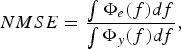 $$NMSE = \displaystyle{\vint \Phi_e \lpar f\rpar df \over \vint \Phi_y \lpar f\rpar df}\comma \;$$
where Φe(f) is the spectrum of the model error e LP(t) = y LP(n) − y mod, LP(n) and Φy(f) is the spectrum of the measured output signal. The integrations are carried out over the available bandwidth.
The ACEPR is given by
 $$ACEPR = \displaystyle{\vint_{max.\; adj.\; ch.} \Phi_e \lpar f\rpar df \over \vint_{ch.} \Phi_y \lpar f\rpar df}\comma \;$$
where the integration in the numerator is performed over the adjacent channel with the largest power and the integration in the denominator is performed over the channel containing the signal. The channel bandwidth is in this case 5 MHz, similar to the 3GPP specifications for ACPR [5].
It is impractical to show the NMSE and ACEPR versus a given nonlinear order or memory depth due to the large number of possible combinations. Therefore, we have chosen to compare the performance (NMSE and ACEPR) as functions of the number of complex-valued model parameters using the convex hull. The settings of nonlinear order and memory depths that result in the convex hull are then separately reported to give an idea of which has the largest influence, memory depth or nonlinear order.
The approach is motivated by two reasons. One is that the complexity in terms of memory and computational load is approximately proportional to the number of parameters when the models have some structure [Reference Soltani Tehrani, Cao, Afsardoost, Eriksson, Isaksson and Fager32]. As an example consider the model x(n)(a 0|x(n − 0)|2 + a 1|x(n − 1)|2) with signal x(n) and (known) parameters a 0 and a 1. When n goes from 1 to 2 the term |x(1)|2 can be re-used. This was the approach taken in [Reference Soltani Tehrani, Cao, Afsardoost, Eriksson, Isaksson and Fager32] by evaluating the number of floating-points operations that a model of given order (nonlinear order and memory depth) needs when it is evaluated. The second motivation comes from the parsimony principle [Reference Söderström and Stoica27] which (simplified) states that of two models with the same performance the simplest model should be used. This is because the variance of the parameter estimates in general increases when more parameters are estimated from a given set of noisy data [Reference Söderström and Stoica27, Reference Kay33]. Thus, model performance is evaluated by considering NMSE and ACEPR as functions of the number of model parameters.
The chosen error criterion for parameter extraction is the standard sum-square error. Thus, for models that are linear in the parameters, the standard linear least-squares method can be used for parameter extraction. To reduce the problems with badly conditioned regression matrices, a scaling and shifting [Reference Golub and Van Loan34], and the SVD in Matlab is used.
All models are extracted using “compact memory” [Reference Ku and Kenney35], i.e. all memory taps are considered to contain information. In [Reference Ku and Kenney35], it was proposed that a sparse modeling approach based on the iterative selection of the taps that result in the lowest model error, thus reducing the number of required model parameters, be used. Another approach to achieve similar results is the use of the LASSO method for parameter extraction, as in [Reference Wisell, Jalden and Händel36].
B) Performance comparison
Results from the modeling in the form of NMSE and ACEPR are compared using the method of plotting the convex hull, as proposed in [Reference Soltani Tehrani, Cao, Afsardoost, Eriksson, Isaksson and Fager32]. The motivation behind this method is that for a given model complexity, in this case, the number of parameters, we are interested in the model that has the lowest model error. In general, there are a large number of parameter settings (choice of nonlinear orders and memory depths) that do not result in low complexity or low model error. However, there is in general no interest in using such a model. Thus, the only models of interest are those on the boundary of model error and complexity.
The convex hulls of the NMSE and ACEPR for the Ericsson PA are presented in Fig. 4. For the NMSE, the MNOMP has the lowest model error when more than 50 complex-valued parameters are considered, with lowest NMSE of −40 dB. This is more than 0.5 dB lower than the EEMP, EPH, and GMP give. For less than 50 complex-valued parameters, the lowest NMSE is given by the EEMP model, with MNOMP giving the second lowest NMSE.
Convex hull of the NMSE and ACEPR for the different models presented earlier versus the number of parameters for the Ericsson PA. (a) NMSE Ericsson PA, (b) ACEPR Ericsson PA.
The de facto standard PH model has the highest NMSE independent of the number of parameters. The largest difference in terms of NMSE between the EEMP and any of the models introduced in Section IV(C), PH, GMP, “full” GMP, EPH, and EMP, occurs for 22 parameters and is more than 1 dB.
For the ACEPR shown in Fig. 4, the EEMP, MNOMP, and GMP models are within 0.1 dB for less than 30 parameters. For more than 50 parameters the MNOMP has between 1 and 1.5 dB lower ACEPR compared to the GMP. For 30–50 parameters the MNOMP and EEMP are similar, approximately 0.5 dB lower ACEPR than the GMP.
For the EEMP models with the lowest NMSE, i.e. those on the complexity-model error boundary, the M 1 is low, typically 1–2 for models with less than 30 parameters. For the MNOMP and the models that are on the complexity-model error boundary, P ranges from 9 to 13, R is 4, M 1 ranges from 1 to 2, and M 2 from 6 to 8. Note that this is for this particular PA.
Results in the form of the convex hull of the NMSE and ACEPR for validation data from the Mini-Circuits amplifier are presented in Fig. 5. The PH model has the highest NMSE of all models, independent of the number of parameters. The EMP model has higher NMSE than the remaining models, except for the full GMP when less than 17 parameters are used. Independent of the parameter count, the EEMP model has the lowest NMSE. The largest difference is on the order of 0.7 dB for about 10 parameters. However, for the EEMP, EPH, GMP, and MNOMP, the differences in NMSE disappear when more than 30 parameters are used.
Convex hull of the NMSE and ACEPR for the different models presented earlier versus the number of parameters for the Mini-Circuits ZVE-8 G amplifier. (a) NMSE ZVE-8G, (b) ACEPR ZVE-8G.
Concerning the ACEPR in Fig. 5, the EEMP has the lowest values for less than 30 parameters, ranging from −55 to −62.5 dB. For more than 30 parameters, the MNOMP model has lower ACEPR values ranging from −63 to −65 dB for more than 100 parameters. The EMP model has 7–10 dB higher ACEPR than all of the other models, except the PH where the difference is on the order of 2 dB.
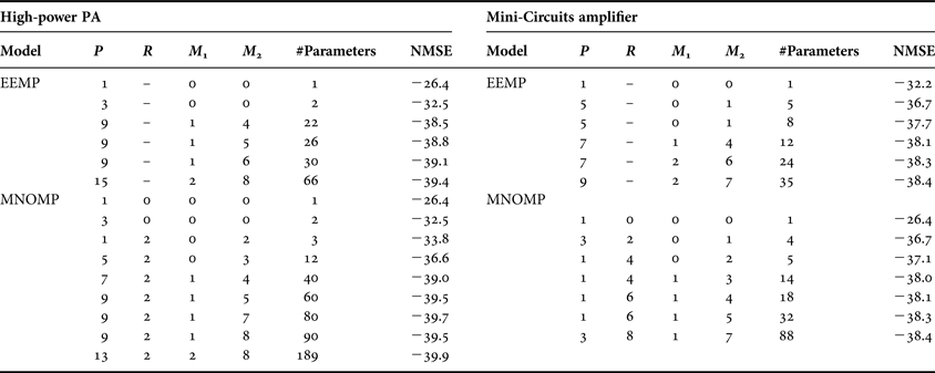
The parameters settings for the EEMP and MNOMP models forming the convex hull of the NMSE for both amplifiers are shown in Table 1. Because the MNOMP and EEMP models consistently provide lower model errors for any given number of parameters only these two models are commented upon in detail here.
Parameter settings for EEMP and MNOMP forming the convex hull.
For the Ericsson high-power PA, the MNOMP finds the nonlinear crossterms x(n)|x(n − m 2)|2 to be important already at three parameters. Note that this is actually an EMP (3,2) model. The MNOMP continues to use crossterms of the type  $x\lpar n - m_1\rpar \vert x\lpar n - m_1\rpar \vert^{2\lpar p - 1\rpar } \vert x\lpar n - m_1 - m_2\rpar \vert^2$. M 1 is mostly 1 which again indicates that terms involving products of different memory depths are more important than products of terms with the same memory depth, as those found in the PH model. For the EEMP model, it can be noted that linear memory M 1 is not of prime concern, but the nonlinear memory terms M 2 are.
For the models obtained using data measured on the Mini-Circuits ZVE-8 G amplifier the parameter settings for the EEMP do not differ significantly. The main difference is that the nonlinear order does not have to be equally high to reach the lowest NMSE. However, for the MNOMP model there is a substantial difference with how the nonlinear memory terms appear. For this amplifier, R is high whereas P is low, quite contrary to the high-power PA. Considering that these terms come from the feedback, it seems that this amplifier has significantly more feedback effects than the high-power PA. The memory depths M 1 and M 2 show no significant differences.
C) Discussion
Clearly, the MNOMP results in the lowest model error, both in band and out of band, but requires a large number of parameters to do so. The EEMP model has a lower model error, NMSE and ACEPR, than the other models when less than 32 parameters are considered. For the particular high-power PA and power level used, the PH model has an NMSE that is approximately 4 dB larger and an ACEPR that is 3 dB larger compared to those of the EEMP models, even when using a larger number of parameters.
In [Reference R”onnow, Wisell and Isaksson37], a three-tone signal was used to directly measure the third-order Volterra kernel of the high-power PA. According to the results in [Reference R”onnow, Wisell and Isaksson37], the dominant symmetry in the third-order Volterra kernel is of the form H 3 = H L(ω 1)H L(ω 2 − ω 3) with H L(ω 1) = C, where C is a constant. ωi, i ∈ {1,2,3} are the frequencies of the input tones, H 3 is the third-order kernel and H L is the frequency response. The frequency dependence of H L close to the carrier is small, hence H L(ω 1) = C. The continuous-time version of the third-order response found in [Reference R”onnow, Wisell and Isaksson37] can thus be expressed as
 $$y_3 \lpar t\rpar = u\lpar t\rpar \vint h_L \lpar \tau\rpar u \lpar t - \tau\rpar u^{\ast} \lpar t - \tau\rpar d \tau\comma \;$$
where h L is the impulse response of H L. Comparing this to the third-order response of the EMP and EEMP models which is of the form  $\sum\nolimits_{m = 0}^M\, g_{3\comma m} u \lpar n\rpar \vert u\lpar n - m\rpar \vert^2$, these are found to share the same symmetry.
In [Reference R”onnow, Wisell and Isaksson37], it is further stated that “The term describes the effect showing that the cascaded quadratic nonlinearities cause a downconversion to the baseband and upconversion to f c. Any baseband frequency dependence of H Lwill thus cause frequency dependence of H 3that can be measured around f c”. The effect of downconversion to baseband and filtering followed by upconversion is the effect of a Hammerstein–Wiener system, which is what is obtained by assuming that the feedback loop is broken, as was also noted in [Reference Pedro and Maas18].
The terms contained in the EEMP model can also be found in both the EPH and GMP models. However, neither of those models can exactly represent the EEMP model by only varying the nonlinear order P and memory depths M 1 and M 2. Additional terms will always be present. Estimating those terms lead to increased parameter variance and noise-fitting which reduces model performance and increases complexity.
From the results a few conclusions are drawn: the EMP model is not recommended due to its inability to model linear frequency dependence, unless it is known that the PA does not have any significant linear frequency dependence; the MNOMP model gives the best performance among the derived model structures but can require a large number of parameters. The EEMP model results in the lowest NMSE when less than 30 parameters are used and it outperforms all other tested model structures. In particular, it has more than 3 dB lower NMSE compared to the PH model.
The derivations implicitly used a number of assumptions. It is then relevant to question the validity of these assumptions; are they relevant for a PA or merely mathematical constructions? What can be said is that if a PA completely failed to fulfill one of the required assumptions the model performance would be seriously degraded. We do believe that the proposed approach of using available knowledge of the PA in order to design behavioral models is a useful method, and that it can aid in the understanding of the PA nonlinear characteristics.
V. CONCLUSIONS
Based on a physically motivated nonlinear feedback system of a PA two novel MP models, the EEMP and MNOMP, were derived. The performance of these two models is compared to that of well-known MP models from the literature, including the PH and GMP models. Using data measured on two RF amplifiers, one high-power PA and one low-power wideband amplifier, it is shown that the EEMP and MNOMP models have lower model errors for any given number of parameters compared to the models from the literature. The necessary derivations are given in such detail that other model structures can be derived, if it should be desired.
From previous measurements of the PA, the dominating symmetry of the third-order Volterra kernel is known to be of the form CH L(ω 2 − ω 3), which is that of a Hammerstein–Wiener system [Reference R”onnow, Wisell and Isaksson37, Reference Landin38]. This symmetry is the same as the symmetry of the third-order kernel of the EEMP model, which further serves to explain the lower model errors obtained with the EEMP model.
ACKNOWLEDGEMENTS
The authors would like to thank Prof. Daniel Rönnow from University of Gävle for very helpful discussions. This research was funded by a research grant from the Ericsson Research Foundation, by the Swedish Research Council (VR), by a postdoctoral fellowship of the Research Foundation-Flanders (FWO), and by the Flemish Government (Methusalem Fund METH1).
APPENDIX
If the assumption of the feedback filter F(ω) is changed so that it passes signal components at the fundamental and the second harmonic as in [Reference Pedro, Carvalho and Lavrador16], a different model structure results.
Changing the assumption on F(ω) changes (4) into
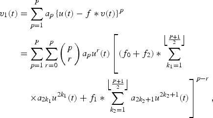 $$\eqalign{v_1 \lpar t\rpar & =\sum\limits_{p = 1}^P a_p \left\{u\lpar t\rpar - f \ast v\lpar t\rpar \right\}^p \cr & = \sum\limits_{p = 1}^P \sum\limits_{r = 0}^p \left(\matrix{ p \cr r} \right)a_p u^r \lpar t\rpar \left[\lpar f_0 + f_2\rpar \ast \sum\limits_{k_1 =1}^{\left\lfloor {P + 1 \over 2} \right\rfloor} \right. \cr & \left. \quad \times a_{2 k_1} u^{2 k_1} \lpar t\rpar + f_1 \ast \sum\limits_{k_2 = 1}^{\left\lfloor {P + 1 \over 2} \right\rfloor} a_{2 k_2 + 1} u^{2 k_2 + 1} \lpar t\rpar \right]^{p - r}\comma \; }$$
if the ordo-term is neglected. f 0 is the part of −F(ω) that passes signal components at baseband, f 1 passes signal components at the fundamental and f 2 at the second harmonic. We choose −F(ω) to remove the negative sign of −f*v(t).
Applying the binomial theorem to (A.1) results in
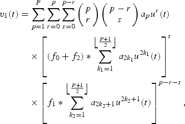 $$\eqalign{v_1 \lpar t\rpar &= \sum\limits_{p = 1}^P \sum\limits_{r = 0}^p \sum\limits_{s = 0}^{p - r} \left(\matrix{ p \cr r} \right)\left(\matrix{p - r \cr s} \right)a_p u^r \lpar t\rpar \cr & \quad \times \left[\lpar f_0 + f_2\rpar \ast \sum\limits_{k_1 = 1}^{\left\lfloor {P + 1 \over 2} \right\rfloor} a_{2 k_1} u^{2 k_1} \lpar t\rpar \right]^s \cr & \quad \times \left[f_1 \ast \sum\limits_{k_2 = 1}^{\left\lfloor {P + 1 \over 2} \right\rfloor} a_{2 k_2 + 1} u^{2k_2 + 1} \lpar t\rpar \right]^{p - r - s}\comma \; }$$
where the bracket containing (f 0 + f 2) has even order signal components and the bracket with f 1 has odd order components. There is no difference in the appearance of the equations if the second order harmonic is allowed to pass F(ω). However, if the first harmonic is also fed back, the model complexity is increased because the last term involving f 1 also has to be modeled.
Per N. Landin received M.Sc. degree in Engineering Physics from Uppsala University, Sweden, in 2007 and the Ph.D. degree in Telecommunication in 2012 jointly from KTH Royal Institute of Technology, Sweden, and Vrije Universiteit Brussel, Belgium. He is currently working as a post-doc at Chalmers University of Technology, Gothenburg, Sweden. His main research interests are in the field of nonlinear high-frequency systems and measurement techniques.
Kurt Barbè received the M.Sc. degree in Mathematics (option Statistics) and the Ph.D. degree in Electrical Engineering from the Vrije Universiteit Brussel (VUB), Brussels, Belgium, in 2005 and 2009, respectively. Presently, he is a Research Professor at the VUB, Department ELEC. Furthermore, he is a post-doctoral research fellow in the Flemish Research Foundation (FWO). His main interests are in the field of system identification, time series analysis and signal processing for biomedical applications. Since 2010, he has served as an associate editor for the IEEE Transactions on Instrumentation and Measurement and since 2013, he joined the editorial board of the journals “Journal of Stochastics” and “The scientific world: probability and statistics”. He is the recipient of the 2011 outstanding young engineer award from the IEEE Instrumentation and Measurement Society and the 2013 Andi Chi Best Paper Award of the IEEE Transactions on Instrumentation and Measurement.
Wendy Van Moer received the M. Eng. and Ph.D. degrees in Engineering from the Vrije Universiteit Brussel (VUB), Brussels, Belgium, in 1997 and 2001, respectively. She is currently an Associate Professor with the Department of Electrical Measurement (ELEC), VUB, and a visiting Professor at the Department of Electronics, Mathematics and Natural Sciences, University of Gävle, Sweden. Her main research interests are nonlinear measurement and modeling techniques for medical and high-frequency applications. Dr. Van Moer was the recipient of the 2006 Outstanding Young Engineer Award from the IEEE Instrumentation and Measurement Society. Since 2007, she has been an Associate Editor for the IEEE Transactions on Instrumentation and Measurement. From 2010 to 2012, she was an Associate Editor for the IEEE Transactions on Microwave Theory and Techniques. In 2012, she was elected as a member of the administrative committee of the IEEE Instrumentation and Measurement society for a 4-year term. In 2014, she became the editor-in-chief of the IEEE Instrumentation and Measurement Magazine.
Magnus Isaksson received the M.Sc. degree in microwave engineering from the University of Gävle, Sweden, in 2000, the Licentiate degree from Uppsala University, Uppsala, Sweden, in 2006, and the Ph.D. degree from the Royal Institute of Technology (KTH), Stockholm, Sweden, in 2007. Isaksson was appointed Docent in 2012, Royal Institute of Technology (KTH), Stockholm, Sweden. He worked on communication products with the Televerket, Sweden, during 1989–1999. He is a teacher in signal processing for Telecommunications and is currently the Head of the Department of Electronics, Mathematics, and Natural sciences at the University of Gävle. His main interests are in signal processing algorithms for radio-frequency measurements and modeling of nonlinear microwave systems. Dr. Isaksson is the author or co-author of many published peer-review journal articles, books, and conference proceedings in the area, and is currently Head of research within the fields of Mathematics, and Natural sciences at the University of Gävle, Sweden.
Peter Händel received the M.Sc. degree in Engineering Physics and the Lic.Eng. and Ph.D. degrees in Automatic Control, all from the Department of Information Technology, Uppsala University, Uppsala, Sweden, in 1987, 1991, and 1993, respectively. During 1987–88, he was a Research Assistant at The Svedberg Laboratory, Uppsala University. Between 1988 and 1993, he was a Teaching and Research Assistant at the Systems and Control Group, Uppsala University. In 1996, he was appointed as Docent at Uppsala University. During 1993–97, he was with the Research and Development Division, Ericsson Radio Systems AB, Kista, Sweden. During the academic year 1996/1997, Dr. Händel was a Visiting Scholar at the Signal Processing Laboratory, Tampere University of Technology, Tampere, Finland. In 1998, he was appointed as Docent at the same university. Since August 1997, he has been in the School of Electrical Engineering, Royal Institute of Technology (KTH), Stockholm, Sweden, where he currently is Professor of Signal Processing and Head of the Department of Signal Processing.