





1 Introduction and main results
1.1 The Willmore energy
For a closed surface
$ \Sigma $
 and an immersion
$ f:\Sigma \to \mathbb {R}^3 $
 into Euclidean space, the Willmore energy is given by

where
$ \mu _f $
 is the area measure induced by
$ f $
 and
$ H=\frac 12 \left (\kappa _1 + \kappa _2\right ) $
 is the mean curvature of
$ f $
 . In this paper, we concentrate on immersed spheres, that is,
$ \Sigma =\mathbb {S}^2 $
 .
The Willmore energy is of considerable analytic interest: its associated Euler–Lagrange equations are a system of quasi-linear, fourth-order partial differential equations. The search for minimizers of the Willmore energy [Reference Li and Yau37, Reference Pinkall and Sterling57, Reference Simon63, Reference Bauer and Kuwert3, Reference Rivière58, Reference Bernard and Rivière5, Reference Marques and Neves40], as well as the study of the corresponding
$ L^2 $
 -gradient flow – the Willmore flow [Reference Kuwert and Schätzle30, Reference Kuwert and Schätzle29, Reference Simonett64, Reference Kuwert and Schätzle31, Reference Lamm and Nguyen33, Reference Langer and Singer35, Reference Dall’Acqua, Müller, Schätzle and Spener11, Reference Palmurella and Rivière54, Reference Dall’Acqua, Müller, Rupp and Schlierf12] – has been the focus of extensive recent study. From a geometric perspective, the Willmore energy is remarkable in being invariant under scaling and conformal transformations; in fact, up to a topological constant, it is the unique global invariant with this full conformal invariance [Reference Mondino and Nguyen48]. It also serves as a bending energy and a measure of complexity as it penalizes self-intersections and deviations from round spheres, making it relevant in applications across biology, physics and computer graphics [Reference Helfrich18, Reference Musielak53, Reference Koerber23, Reference Botsch, Kobbelt, Pauly, Alliez and Levy7]. We refer the reader to [Reference Kuwert and Schätzle32, Reference Rivière60, Reference Marques and Neves41] for an overview of the Willmore energy and its applications.
In the following section, we outline the approach taken in this paper and relate it to known results. The main contribution of this paper is stated in Section 1.3 as Theorem 1.2, with further results and applications in Sections 1.4, 1.5, 1.6 and 1.7. The remaining sections are mostly dedicated to the proof of Theorem 1.2.
1.2 The Willmore energy landscape
An energy landscape is the graph of an energy function over a set of admissible objects, in this case the Willmore functional over the set
$ \text {Imm}(\mathbb {S}^2,\mathbb {R}^3) $
 of smoothly immersed
$ 2 $
 -spheres in Euclidean
$ 3 $
 -space. Usually, a landscape is described by its critical points and their indices. The Willmore energy landscape of spheres has been thoroughly studied from this Morse-theoretic viewpoint. All its immersed critical points, the Willmore spheres, are classified [Reference Bryant9]. They are inverted complete minimal surfaces with finite total curvature and embedded planar ends and appear at quantized energy levels
$ 4\pi k $
 for some
$ k\in \mathbb {N} $
 . The absolute minima at
$ 4\pi $
 are the round spheres, that is, reparametrizations, scalings and translations of the standard embedding
$ e:\mathbb {S}^2\to \mathbb {R}^3 $
 . After
$ 4\pi $
 , the next Willmore spheres appear at
$ 16\pi $
 . They form a four-parameter family up to reparametrization and conformal transformation [Reference Bryant9] and their indices are equal to one [Reference Hirsch and Mäder-Baumdicker21, Reference Hirsch, Kusner and Mäder-Baumdicker20]. Beyond smoothly immersed Willmore spheres, branched Willmore spheres have been the subject of recent research [Reference Kuwert and Li27, Reference Chen and Li10, Reference Lamm and Nguyen33, Reference Michelat45, Reference Michelat and Rivière46, Reference Martino42] (with differing notions of “branched”, see [Reference Martino42]). These results all provide local information about the energy landscape.
The main object of this paper is to obtain insight into the global topology of the Willmore energy landscape. One approach is to cut off the landscape at certain energy levels and analyze the structure of the resulting “valleys”, that is, the regular homotopy classes of the sublevel sets

for
$ \omega \geq 4\pi $
 . A purely topological result by Smale shows that the whole space
$ I(\infty )=\text {Imm}(\mathbb {S}^2,\mathbb {R}^3) $
 has one regular homotopy class [Reference Smale65]. But to tackle the question for finite energy values, one has to combine tools from topology and geometric analysis.
For
$ \omega \leq 8\pi $
 , such tools are available and they imply

To prove this, we first employ the Willmore flow to get an upper bound on the number of regular homotopy classes of
$ I(\omega ) $
 . Kuwert and Schätzle proved that, up to
$ 8\pi $
 , the Willmore flow behaves well.
Theorem A [Reference Kuwert and Schätzle31].
Let
$ f_0:\mathbb {S}^2\to \mathbb {R}^3 $
 be a smooth immersion of a sphere with Willmore energy

Then, the Willmore flow with initial data
$ f_0 $
 exists smoothly for all times and converges to a round sphere.
Recall that all orientation-preserving diffeomorphisms of
$ \mathbb {S}^2 $
 are homotopic to each other [Reference Smale66] and thus Theorem A implies that
$ I(8\pi ) $
 has at most two regular homotopy classes, since every
$ f\in I(8\pi ) $
 can be joined to a round sphere of either orientation by the Willmore flow.
Second, a lower bound on the number of regular homotopy classes of
$ I(\omega ) $
 arises from a topological study of self-intersections carried out by Max and Banchoff [Reference Max and Banchoff43] (with alternative proofs [Reference Hughes22, Reference Goryunov17]). We say that a regular homotopy
$ f:\mathbb {S}^2\times [0,1]\to \mathbb {R}^3 $
 has an n -tuple point if there exist
$ t\in [0,1] $
 and
$ x\in \mathbb {R}^3 $
 such that
$ \left (f(\cdot ,t)\right )^{-1}(\{x\}) $
 contains at least
$ n $
 points.
Theorem B [Reference Max and Banchoff43].
Every regular homotopy between two round spheres of opposite orientation has a quadruple point.
The decisive link between the topology of self-intersections and the Willmore energy is the Li–Yau inequality.
Theorem C [Reference Li and Yau37].
If a smooth immersion
$ f:\Sigma \to \mathbb {R}^k $
 of a closed surface has an
$ n $
 -tuple point, then

As a consequence, every regular homotopy between two round spheres of opposite orientation must pass through a time at which the immersion has Willmore energy at least
$16\pi $
 . Thus, round spheres of opposite orientation cannot lie in the same regular homotopy class in
$ I(\omega ) $
 for
$ \omega <16\pi $
 . Consequently, for
$ \omega \in [4\pi ,16\pi ) $
 , the sublevel set
$ I(\omega ) $
 has at least two regular homotopy classes. With Theorem A, we arrive at equation (1.1).
The aim of this paper is to extend this approach to
$ \omega \in (8\pi ,12\pi ] $
 , where Theorem A is not available because singularities of the Willmore flow might prevent the convergence to a round sphere.
1.3 Main results
For any immersion
$ f:\mathbb {S}^2\to \mathbb {R}^3 $
 , we denote by
$ -f $
 the immersion defined by
$ (-f)(x):=-f(x) $
 .
Definition 1.1. Consider a smooth immersion
$ j:\mathbb {S}^2\to \mathbb {R}^3 $
 obtained by rotating the curve displayed in Figure 1. Let
$ J $
 be the set of all smooth immersions
$ f:\mathbb {S}^2\to \mathbb {R}^3 $
 that admit a regular homotopy without triple points to
$ j $
 or
$ -j $
 .
In [Reference Mayer and Simonett44, Reference Blatt6], surfaces of revolution of this kind serve as initial surfaces that lead to singularities. However, surfaces in
$ J $
 are not necessarily rotationally symmetric and may possess additional self-intersections. In fact, the definition of
$ J $
 is rather implicit, but note that for any given smooth immersion
$ f:\mathbb {S}^2\to \mathbb {R}^3 $
 , an invariant devised in [Reference Seidel62] gives an explicit way of checking whether
$ f $
 belongs to
$ J $
 .
We show that
$ J $
 defines model surfaces that can be reached by regular homotopies of low Willmore energy whenever the Willmore flow fails to converge to a round sphere. The proof relies crucially on the classification of blow-ups at the singular time by Lamm and Nguyen [Reference Lamm and Nguyen33]. The main contribution of this paper is the following (see Section 2.3 for the proof). For homotopies
$ H:\mathbb {S}^2\times I \to \mathbb {R}^3 $
 , we denote
$ H_t:=H(\cdot ,t) $
 .
Theorem 1.2. If a smooth immersion
$ f:\mathbb{S}^2 \to \mathbb{R}^3 $
 has Willmore energy
$ W(f) \in (4\pi, 12\pi ] $
 , then there exists a regular homotopy
$ H: \mathbb{S}^2 \times [0,1] \to \mathbb{R}^3 $
 which satisfies
$ H_0 = f $
 ,
$ W(H_t) < W(f) $
 for all
$ t \in (0,1] $
 and
$ H_1 $
 is either a round sphere or equal to some
$ j\in J $
 .
The immersion
$ j $
 in Theorem 1.2 can be taken to have Willmore energy arbitrarily close to
$ 8\pi $
 .
An invariant introduced by the second author in [Reference Seidel62] shows that the model surfaces
$ J $
 cannot be omitted in Theorem 1.2. It relies on the structure of self-intersecting immersed spheres, similar to that revealed in Theorem B, though the invariant is obtained using entirely different methods.
Theorem D [Reference Seidel62, Theorem 1.7].
Every regular homotopy joining some
$ j\in J $
 to an embedded sphere has triple points.
The Li–Yau inequality immediately gives
$ W(H_t)\geq 12\pi $
 for some time
$ t $
 . This can be improved to a strict inequality (see Appendix A).
Corollary 1.3. For every regular homotopy
$ H:\mathbb {S}^2\times [0,1] \to \mathbb {R}^3$
 from some
$ j\in J $
 to an embedded sphere, there exists a time
$ t\in [0,1] $
 with
$ W(H_t)>12\pi $
 .
The two theorems combined yield the following.
Theorem 1.4.
$ I(\omega ) $
 has four regular homotopy classes for
$ \omega \in (8\pi ,12\pi ] $
 .
An immersion in the family
$ J $
 and its generating curve.

A sketch of the Willmore energy landscape of immersed
$ 2 $
 -spheres in
$ \mathbb {R}^3 $
 below
$ 12\pi $
 .

Figure 2 Long description
The diagram features four light-gray shaded V-shaped regions arranged horizontally. Three horizontal dotted lines serve as energy level markers.
* The lowest dotted line is labeled 4 pi on the right. Two large V-shaped wells in the center have their vertices touching this line. Below the left central vertex is an orange sphere, and below the right central vertex is a purple sphere.
* The middle dotted line is labeled 8 pi on the right. Two smaller V-shaped wells, one on the far left and one on the far right, have their vertices touching this line.
* The top dotted line is labeled 12 pi on the right. This line marks the upper boundary for all four V-shaped regions.
Inside the far-left well, near the 12 pi line, are two overlapping orange and purple spheres. Similarly, inside the far-right well, near the 12 pi line, are two overlapping orange and purple spheres. The central two wells are empty of spheres within their shaded regions.
Proof of Theorem 1.4.
As a consequence of Theorem 1.2, there exists
$ j\in J \, \cap \, I(\omega ) $
 such that all
$ f\in I(\omega ) $
 can be joined to
$ j $
 ,
$ -j $
 ,
$ e $
 or
$ -e $
 by a regular homotopy in
$ I(\omega ) $
 (see Lemma 2.8). Therefore,
$ I(\omega ) $
 has at most four regular homotopy classes. In
$ I(\omega ) $
 , the immersion
$ j $
 is not regularly homotopic to
$ -j $
 since all regular homotopies from any
$ f\in \text {Imm}(\mathbb {S}^2,\mathbb {R}^3) $
 to
$ -f $
 have a quadruple point [Reference Max and Banchoff43]. By Corollary 1.3, it is also not regularly homotopic to
$ e $
 or
$ -e $
 in
$ I(\omega ) $
 . This proves the statement.
In the two regular homotopy classes
$ J_+ $
 and
$ J_- $
 that do not contain round spheres, the infimum

is not attained (see Remark 2.9).
1.4 Avoidable singularities
For every initial surface, there exists a Willmore flow
$ f:\mathbb {S}^2\times [0,T)\to \mathbb {R}^3 $
 on a maximal interval
$ [0,T) $
 with
$ 0<T\leq \infty $
 [Reference Kuwert and Schätzle32]. If
$ T<\infty $
 , then
$ f $
 cannot be smoothly extended onto
$ T $
 .
Definition 1.5. We say that a maximal Willmore flow
$ f:\mathbb {S}^2\times [0,T)\to \mathbb {R}^3 $
 develops a singularity if it does not converge smoothly to a Willmore sphere as
$ t\to T $
 . This singularity is avoidable if there exists a regular homotopy
$ H:\mathbb {S}^2 \times [0,1]\to \mathbb {R}^3 $
 from
$ f_0 $
 to a smooth Willmore sphere with
$ W(H_t)<W(f_0) $
 for all
$ t\in (0,1] $
 . If no such homotopy exists, we call the singularity unavoidable.
Recall that below
$ 16\pi $
 the only smooth Willmore spheres are the round spheres [Reference Bryant9]. Whether the Willmore flow can develop singularities in finite time, and whether the area remains bounded, are both open questions. No such assumptions are imposed in the definition.
Blatt showed in [Reference Blatt6] that the Willmore flow starting in certain surfaces of revolution in
$ J $
 necessarily develops singularities. If it were to converge to a round sphere, this would imply the existence of a regular homotopy between plane curves of different turning numbers. This example was originally proposed in [Reference Mayer and Simonett44], where numerical simulations suggested singularity formation in finite time. In [Reference Dall’Acqua, Müller, Schätzle and Spener11], a family of singular examples for tori of revolution was given following an analogous argument. Apart from surfaces of revolution, no other initial surfaces are currently known to produce singularities under the Willmore flow. As a consequence of Theorem D, not only do surfaces of revolution in
$ J $
 develop singularities under the Willmore flow, but so does any other initial surface in
$ J $
 . We obtain a full classification of initial surfaces with energy at most
$ 12\pi $
 that lead to unavoidable singularities.
Proposition 1.6. Let
$ f_0:\mathbb {S}^2\to \mathbb {R}^3 $
 be a smooth immersion with
$ W(f_0) \leq 12\pi $
 . Then, the Willmore flow with initial surface
$ f_0 $
 develops an unavoidable singularity if and only if
$ f_0\in J $
 .
Proof. If
$ f_0\in J $
 , then, by Theorem D, its Willmore flow necessarily develops an unavoidable singularity; otherwise, it would provide a regular homotopy to a round sphere without triple points. If, conversely, the Willmore flow with initial surface
$ f_0 $
 develops an unavoidable singularity, then, by Theorem 1.2, there exists a regular homotopy
$ H $
 with
$ W(H_t) < W(f_0) $
 for
$ t\in (0,1] $
 , ending in some
$ j\in J$
 . In particular,
$ H $
 has no triple points, and it follows that
$ f_0\in J $
 .
These results do not describe the analytic behavior of the Willmore flow. In particular, it remains open whether the Willmore flow can develop avoidable singularities. However, it seems reasonable to expect that singularity formation is governed not only by the global topology of self-intersections but also by local analytic behavior.
Conjecture 1.7. There exists a smooth immersion
$ f_0:\mathbb {S}^2\to \mathbb {R}^3 $
 with
$ W(f_0)\leq 12\pi $
 such that the Willmore flow with initial surface
$ f_0 $
 develops an avoidable singularity.
One might find an initial surface
$ f_0\notin J $
 that locally is very close to a catenoid singularity (e.g., three of the four cases in Figure 4). One would need to show that such a (global) singularity model indeed appears as a singularity of the flow. Similar arguments have been made for the Ricci flow [Reference Stolarski67] and the mean curvature flow [Reference Lee and Zhao36]. However, these flows develop singularities in finite time, whereas it remains an open question whether the Willmore flow does as well.

1.5 An extension of the Li–Yau inequality at
$ 12\pi $


The Li–Yau inequality provides a rare and powerful link between the global topology of an immersed surface – particularly its self-intersections – and its Willmore energy, an integral of a fundamentally local quantity. It has also been extended to related settings, such as for curves [Reference Müller and Rupp51, Reference Miura47] and for surfaces with boundary [Reference Schlierf61].
The Li–Yau inequality supports the idea that Willmore energy serves as a measure of complexity: more “complicated” immersions tend to have higher Willmore energy. An immersion with a triple point, for instance, has Willmore energy at least
$ 12\pi $
 . Similarly, an immersion with arbitrarily short closed geodesic has Willmore energy at least
$ 6\pi $
 [Reference Müller, Rupp and Scharrer52]. Taking genus into account, the Willmore Conjecture states that every immersed torus has Willmore energy at least
$ 2\pi ^2 $
 . The Li–Yau inequality reduces the problem to embedded tori, and the conjecture was famously resolved by Marques and Neves [Reference Marques and Neves40]. Moreover, the minimal energy for fixed genus
$ g $
 tends to
$ 8\pi $
 as
$ g\to \infty $
 [Reference Kuwert, Li and Schätzle28].
However, beyond the relations to genus and the Li–Yau inequality, such direct connections between the topological complexity of a closed surface and its Willmore energy remain rare. We present two results in this spirit. The first is a lower bound of
$ 12\pi $
 for a large family of surfaces without triple points; the second is a lower bound for spheres of revolution in terms of the turning number of the generating curve. Both results crucially depend on the Li–Yau inequality.
Theorems 1.2 and D provide an explicit description of the self-intersections of immersed spheres with Willmore energy at most
$ 12\pi $
 . This yields the following extension of the Li–Yau inequality at
$ 12\pi $
 . We denote by

the invariant defined in [Reference Seidel62] and by
$ e_k:=(\delta _{ik})_{i\in \mathbb {Z}} $
 the standard basis vectors of
$ \mathbb {Z}^{\mathbb {Z}} $
 .
Proposition 1.9. Let
$ f:\mathbb {S}^2\to \mathbb {R}^3 $
 be a smooth immersion without triple points. If
$ F(f)\notin \{e_{-3},e_{-1},e_1,e_3\} $
 , then
$ W(f)> 12\pi $
 .
Proof. Suppose
$ W(f)\leq 12\pi $
 . In [Reference Seidel62, Example 5.2], it is computed that
$ F(\pm e)=e_{\pm 1} $
 and
$ F(j)=e_{\pm 3} $
 for all
$ j\in J $
 . Then, Theorem 1.2 provides a regular homotopy without triple points to round spheres
$ e $
 ,
$ -e $
 or some
$ j\in J $
 . The invariant is constant along regular homotopies without triple points [Reference Seidel62, Theorem 1.3] and thus
$ F(f)\in \{e_{-3},e_{-1},e_1,e_3\}. $

The assumptions of Proposition 1.9 are satisfied by a large family of immersions. See [Reference Seidel62, Section 6] for a description of the image of
$ F $
 and Figure 3 for some examples. Note that the proposition applies not only to the displayed surfaces but also to any deformation without triple points that may break any symmetry.
Some immersions without triple points and their values of
$ F $
 as computed in [Reference Seidel62, Figure 17].

Figure 3 Long description
The diagram consists of four panels arranged horizontally. A horizontal axis line passes through the first three panels, with a rotational arrow on the far left indicating symmetry.
* The first panel on the left shows a blue curve forming three interconnected loops symmetric across the axis. Below it is the formula F = 2 e sub 3 minus e sub 1.
* The second panel shows two large circular lobes that meet at the axis, with a small vertical arrow pointing upward from the top of the left lobe. Below it is the formula F = 2 e sub 1 minus e sub negative 1.
* The third panel shows a complex curve with two large outer loops and two smaller inner loops crossing the axis, with a vertical arrow on the top left loop. Below it is the formula F = e sub 3 plus e sub negative 1 minus e sub 1.
* The fourth panel on the far right depicts a three-dimensional surface resembling three spheres connected by a central hub, with a small vertical arrow at the center. Below it is the formula F = 3 e sub negative 1 minus 2 e sub 1.
We mention one further extension of the Li–Yau inequality that is independent of the other results in this paper. It applies only to spheres of revolution. A sphere of revolution is a smoothly immersed sphere that can be parametrized as
$ f(t,\varphi )= \left (r(t)\cos \varphi ,r(t)\sin \varphi ,h(t)\right )$
 for some regular curve
$ c=(r,h):[0,1]\to [0,\infty )\times \mathbb {R} $
 where
$ r(0)=r(1)=0 $
 ,
$ r(t)>0 $
 for all
$ t\in (0,1) $
 and
$ c $
 meets the symmetry axis perpendicularly.
Proposition 1.10. Let
$ f:\mathbb {S}^2\to \mathbb {R}^3 $
 be a sphere of revolution whose generating curve
$ c:[0,1]\to [0,\infty )\times \mathbb {R} $
 has turning number
$ \tau \in \mathbb {Z}+\frac 12 $
 . If
$ f $
 is not a round sphere, then

A proof can be found in Appendix A. This inequality is sharp as can be seen from gluing round spheres together by catenoid necks (see Remark 2.9 and [Reference Blatt6] for
$ \left \lvert \tau \right \rvert =\frac 32 $
 ). For tori of revolution, analogous methods yield the (nonsharp) inequality
$ W(f)\geq 4\pi \left \lvert \tau \right \rvert $
 . It is interesting to compare these lower bounds to the energy of Willmore surfaces of revolution (see [Reference Mandel39, eq. (46)]).
1.6 An optimal sphere eversion
We outline the relations of the main results of this paper to sphere eversions and the
$ 16\pi $
 -Conjecture. A sphere eversion is a regular homotopy connecting two round spheres of opposite orientation. The existence of a sphere eversion was proved by Smale [Reference Smale65], and later explicit sphere eversions were found [Reference Kuiper24, Reference Phillips56, Reference Morin and Petit49, Reference Apéry2, Reference Francis, Sullivan and Hartman14, Reference Aitchison1, Reference Hirasawa and Yamamoto19, Reference Bednorz and Bednorz4], the first by Shapiro [Reference Francis and Morin16]. Theorem B by Max and Banchoff shows that for every sphere eversion
$ H $
 , there exists
$ t\in [0,1] $
 such that
$ H_t $
 has a quadruple point. By the Li–Yau inequality, it follows that
$ W(H_t)\geq 16\pi $
 . Hence, every sphere eversion must reach a Willmore energy of at least
$ 16\pi $
 . Does there exist an optimal sphere eversion in the following sense?
16π-Conjecture (Kusner, 1984).
There exists a sphere eversion
$ H:\mathbb {S}^2\times [0,1]\to \mathbb {R}^3 $
 that satisfies for all
$ t\in [0,1] $


Kusner proposed to construct such an optimal sphere eversion by a min-max procedure or by Willmore flow. We summarize the idea of the latter here while the former is treated in [Reference Rivière59]. One explicit sphere eversion is the Froissart-Morin sphere eversion [Reference Morin and Petit49], which uses Morin’s surface [Reference Morin and Petit50] as a halfway model. It has the special symmetry that, after a rotation of
$ \frac \pi 2 $
 in
$ \mathbb {R}^3 $
 , the same surface is obtained but of opposite orientation. Given a regular homotopy from such a halfway model to a round sphere, one obtains a sphere eversion whose second half is constructed by reversing the orientation and the temporal direction of the first half. Kusner found an explicit parametrization of a complete minimal surface whose compactified inversion is the Morin surface and a critical point of the Willmore energy at
$ 16\pi $
 [Reference Kusner25]. This surface can be perturbed along its index-one direction [Reference Hirsch and Mäder-Baumdicker21] to reduce its energy below
$ 16\pi $
 . This perturbed surface is not a critical point and thus the Willmore flow can deform it to reduce the Willmore energy. However, it is not known whether the Willmore flow exists for all time and converges to a round sphere. In [Reference Francis, Sullivan, Kusner, Brakke, Hartman and Chappell15], numerical analysis suggests that it does, but analytically, the possibility of singularities developing under the Willmore flow in this case has not been ruled out.
We obtain the following.
Proposition 1.11. If a smooth immersion
$ f:\mathbb {S}^2\to \mathbb {R}^3 $
 has Willmore energy at most
$ 12\pi $
 and there exists a regular homotopy from
$ f $
 to a round sphere without triple points, then there also exists one whose Willmore energy does not exceed
$ W(f) $
 .

In other words, for a given initial surface, the topological description of a regular homotopy to a round sphere is sufficient to obtain a regular homotopy of low Willmore energy.
Question 1.12. Does Proposition 1.11 remain true if “
$ 12\pi $
 ” is replaced by “
$ 16\pi $
 ” and “triple points” is replaced by “quadruple points”?
An affirmative answer to the preceding question would prove the
$ 16\pi $
 -Conjecture since the Froissart-Morin sphere eversion provides a regular homotopy from the perturbed Kusner-Morin surface to a round sphere without quadruple points. This would require a generalization of the main results to
$ 16\pi $
 , which is discussed in the following section.
1.7 Generalizations to
$ 16\pi $

A complete description of the Willmore energy landscape would include the number of regular homotopy classes of the sublevel sets
$ I(\omega ) $
 , not only for
$ \omega \in [4\pi ,12\pi ] $
 , but for all
$ \omega \in [4\pi ,\infty ) $
 . We outline the challenges for the generalization to
$ \omega \leq 16\pi $
 .
Question 1.13. What are the regular homotopy classes of
$ I(\omega ) $
 for
$ \omega \in (12\pi ,16\pi ] $
 ?
Answering this requires a generalization of both Theorem 1.2 and Theorem D. The former can build on the local classification of [Reference Lamm and Nguyen33] up to
$ 16\pi $
 , but challenges arise. See Section 2.4, which contains a partial result. For the latter, instead of an invariant for triple-point-free immersions, one would need to devise an invariant for quadruple-point-free immersions that separates round spheres from any
$ j\in J $
 as well as any other global singularity model that may arise.
Question 1.14 [Reference Seidel62, Question 1.8].
Does every regular homotopy joining some
$ j\in J $
 to an embedded sphere have at least one quadruple point?
Similar results for
$ \omega>16\pi $
 are out of reach for the approach introduced in this paper. This is due to the fact that results like Theorem B and Theorem D can only exist for
$ n $
 -tuple points with
$ n\leq 4 $
 : Any regular homotopy of surfaces immersed in
$ \mathbb {R}^3 $
 can be slightly perturbed to not have any
$ n $
 -tuple points for
$ n\geq 5 $
 (cf. [Reference Seidel62]).
2 Avoiding Singularities of the Willmore Flow
In this section, we give a global description of singularities of the Willmore flow below
$ 12\pi $
 using the local classification of [Reference Lamm and Nguyen33], and prove Theorem 1.2.
We first present the idea of the proof. The details are covered in Sections 2.2 and 2.3. Let
$ f:\mathbb {S}^2 \times [0,T)\to \mathbb {R}^3 $
 be a maximal Willmore flow with
$ W(f_0)\leq 12\pi $
 that does not converge to a round sphere. Then, by [Reference Lamm and Nguyen33], there is a point in
$ \mathbb {R}^3 $
 around which the image of
$ f $
 locally converges to a catenoid. This catenoid may be increasing or decreasing in scale. By scale invariance of the Willmore energy, a homotopy that scales the immersion by some factor
$ \lambda _t $
 with
$ \lambda _0=1 $
 has constant Willmore energy. In the following, we implicitly assume such rescaling whenever needed. At some time
$ s<T $
 , the immersion
$ f_{s} $
 is on some annulus
$ C\subseteq \mathbb {S}^2 $
 sufficiently close to a catenoid [Reference Lamm and Nguyen33]. We replace the catenoid by two flat disks and glue them to
$ f|_{D_1} $
 and
$ f|_{D_2} $
 on the remaining disk components
$ D_1 $
 and
$ D_2 $
 of
$ \mathbb {S}^2\setminus C $
 . We obtain two immersed spheres, each of which has Willmore energy less than
$ 8\pi $
 . This allows us to start the Willmore flow, which converges to a round sphere [Reference Kuwert and Schätzle31]. These two flows are then glued to the two boundaries of the catenoid
$ f|_C $
 at each time. To control the Willmore energy of the gluing, we scale up the two flows as needed. This yields a regular homotopy ending in a small catenoid glued to two round spheres (see Proposition 2.7). Each sphere can be oriented in two ways relative to the catenoid (see Figure 4).
Four ways to attach two round spheres to a catenoid.

In one of the four cases, we obtain an immersion of the family
$ J $
 , and we are done. For the other cases, the catenoid lies outside of at least one of the spheres, and we can decrease the Willmore energy by shrinking this sphere relative to the catenoid (see Lemma 2.4). Over time, we see less of both the sphere and the catenoid and eventually drop below a Willmore energy of
$ 8\pi $
 . We then restart the Willmore flow, which converges to a round sphere.
2.1 Notation
We denote open balls of radius
$ r>0 $
 and center
$ p\in \mathbb {R}^n $
 by
$ B_r(p) $
 . For a smooth map
$ f:\Omega \subseteq \mathbb {R}^m\to \mathbb {R} $
 , we write

and for maps
$ f:\Omega \subseteq \mathbb {S}^2\to \mathbb {R}^3 $
 , we define
$ C^k $
 norms by fixing charts of
$ \mathbb {S}^2 $
 . For an interval of radii
$ I\subseteq (0,\infty ) $
 , we denote an annulus by

2.2 Gluing round spheres to catenoids
For the remainder of this section, we fix for all
$ \delta>0 $
 a gluing function
$\phi \in C^\infty (\mathbb {R},\mathbb {R})$
 with

and the properties
$ \left \lvert \phi \right \rvert \leq 1, \left \lvert \phi '\right \rvert \leq M\delta ^{-1}, \left \lvert \phi "\right \rvert \leq M\delta ^{-2} $
 for some constant
$ M>0 $
 independent of
$ \delta $
 . A standard mollifier serves to construct such a function.
Definition 2.1. For
$ \delta \in (0,1) $
 , the gluing function
$ \phi :\mathbb {R} \to \mathbb {R} $
 , the annulus
$ A:=\operatorname {\mathrm {Ann}}[1-\delta ,1+\delta ] $
 and two graphs
$ f_1,f_2:A\to \mathbb {R}^3 $
 with
$ f_i(x,y) = (x,y,u_i(x,y)) $
 for some
$ u_1,u_2\in C^2(A,\mathbb {R}) $
 , we define the
$ \delta $
 -gluing of
$ f_1 $
 and
$ f_2 $
 as the graph
$ \tilde {f}(x,y)=(x,y,\tilde {u}(x,y)) $
 where
$ \tilde {u} $
 is defined as

Lemma 2.2. Let
$ \delta \in (0,1) $
 . Then, there exists some constant
$ C(M,\delta )>0 $
 such that the following holds. For all
$A,f_1,f_2,u_1,u_2 $
 as above that in addition satisfy
$ \left \lVert u_i\right \rVert _{C^2(A)}\leq 1 $
 , the
$ \delta $
 -gluing
$ \tilde {f} $
 of
$ f_1 $
 and
$ f_2 $
 satisfies

Proof. Consider the involved graphs in polar coordinates
$ (x,y)= r(\cos \varphi ,\sin \varphi ) $
 . Then, the
$ \delta $
 -gluing
$ \tilde {u}(r,\varphi ):=u_1(r,\varphi ) + \phi (r)\left ( u_2(r,\varphi ) - u_1(r,\varphi ) \right ) $
 has the derivatives

Since
$ \delta <1 $
 , we have
$ \left \lvert \phi \right \rvert ,\left \lvert \phi '\right \rvert ,\left \lvert \phi "\right \rvert \leq \frac {M}{\delta ^2} $
 . It follows that

for all multiindices
$ \alpha $
 with
$ \left \lvert \alpha \right \rvert \leq 2 $
 . Furthermore, with the assumption
$ \left \lVert u_i\right \rVert _{C^2(A)}\leq 1$
 , we have

Now, the integrand
$ H^2\sqrt {\det G} $
 of the Willmore energy, with mean curvature
$ H $
 and first fundamental form
$ G $
 , is a differentiable function of the first and second derivatives of
$ u $
 . Thus, it is Lipschitz on the bounded domain specified by equation (2.2) with some Lipschitz constant
$ L(M,\delta )>0 $
 . Together with equation (2.1), we obtain

With the area
$ 4\pi \delta $
 of the annulus, we conclude

Note that there exist other methods for smoothly gluing two surfaces together that are more efficient in terms of Willmore energy; see [Reference Bauer and Kuwert3] for an example. The purpose of the gluing defined above is to provide a simple, explicit construction that nonetheless has controlled Willmore energy.
Let
$\lambda>1, R>1, \delta \in (0,1-1/\lambda )\cap (0,R-1) $
 . We want to define the
$ \delta $
 -gluing of one half of a catenoid of scale
$1/\lambda $
 with a sphere of radius
$ R $
 . First, define

and the curves


The first curve is a catenary and the second the “east” half of a circle of radius R and midpoint
$ (0,R\cos (\theta ))=(0,\sqrt {R^2-1}) $
 . We have
$ c_1(t_0)=c_2(\theta ) = (1,0) $
 . At this intersection point,
$ c_1 $
 and
$ c_2 $
 are tangent if and only if
$ R = \lambda $
 . Let
$ u_1:[1/\lambda , 1+\delta ]\to \mathbb {R} $
 and
$ u_2:[0,R)\to \mathbb {R} $
 be the graph parametrizations of
$ c_1 $
 and
$ c_2 $
 , that is,
$ x\mapsto (x,u_i(x)) $
 parametrizes a part of
$ c_i $
 . We now extend
$ u_1,u_2 $
 to rotationally symmetric functions on annuli and construct the gluing
$ \tilde u : \operatorname {\mathrm {Ann}}[1-\delta , 1+\delta ]\to \mathbb {R} $
 of
$ u_1 $
 and
$ u_2 $
 according to Definition 2.1. Now, define
$ g_\beta (x,y):=(x,y,u_\beta (x,y)) $
 on
$ \operatorname {\mathrm {Ann}}[1/\lambda ,R) $
 with (see also Figure 5)

Let
$ D\subseteq \mathbb {S}^2 $
 be a closed topological disk and
$ f_\beta :D\to \mathbb {R}^3 $
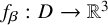 be any smooth immersion such that the interior of
$ D $
 contains a closed disk
$D_1$
 ,
$f_\beta |_{D_1}$
 parametrizes a closed (round) hemisphere of radius R and
$ f_\beta |_{D\setminus D_1} $
 parametrizes the same surface as
$ g_\beta $
 (see Figures 5 and 6). We call
$f_\beta $
 a catenoid sphere of type
$\beta $
 .
The profile curves for the smooth rotationally symmetric catenoid spheres of types
$\alpha $
 and
$\beta $
 .

The gluing region and the functions
$ u_1,u_2,\tilde {u} $
 .

Figure 6 Long description
A two-panel line graph. Both panels feature a horizontal axis with three tick marks labeled 1 minus delta, 1, and 1 plus delta.
Left panel (type alpha)
* A central intersection point is labeled u tilde at the coordinate 1 on the horizontal axis.
* Function u sub 1 is a red dashed line with a positive linear slope.
* Function u sub 2 is a blue dashed line with a negative linear slope.
* Function u tilde is a black dashed curve that forms a concave downward parabola, peaking at the intersection point 1 and following the paths of u sub 1 and u sub 2 as they move away from the center.
Right panel (type beta)
* A central intersection point is labeled u tilde at the coordinate 1.
* Function u sub 1 is a red dashed line with a positive linear slope.
* Function u sub 2 is a blue dashed curve that starts below u sub 1 on the left, intersects at 1, and rises above u sub 1 on the right.
* Function u tilde is a black dashed line that appears to overlap or follow the linear path of u sub 1 through the intersection point.
To define catenoid spheres of type
$\alpha $
 , we repeat the definition above but with the curve
$c_2$
 adjusted to be

This is the “east” half of a circle of radius R and midpoint
$ (0,-R\cos (\theta )) $
 . Again, we have
$ c_1(t_0)=c_2(\theta ) = (1,0) $
 , but
$c_1$
 and
$c_2$
 are never tangent at this intersection point. We proceed analogously with the construction and obtain catenoid spheres
$f_\alpha $
 of type
$ \alpha $
 (see Figure 5).
Definition 2.3. We define
$ \text {CatSph}_\alpha (\lambda ,R,\delta ) $
 (resp.
$ \text {CatSph}_\beta (\lambda ,R,\delta ) $
 ) to be the set of all catenoid spheres
$ f_\alpha $
 (resp.
$ f_\beta $
 ) of type
$ \alpha $
 (resp.
$ \beta $
 ) for given
$\lambda>1$
 ,
$R>1$
 and
$\delta \in (0,1-1/\lambda )\cap (0,R-1)$
 as defined above. We also set

We denote by
$ W_\alpha (\lambda ,R,\delta ) $
 (resp.
$ W_\beta (\lambda ,R,\delta ) $
 ) the Willmore energy of some catenoid sphere
$ f\in \text {CatSph}_\alpha (\lambda ,R,\delta ) $
 (resp.
$ f\in \text {CatSph}_\beta (\lambda ,R,\delta ) $
 ). We extend these functions by

which is the Willmore energy of the spherical region in the catenoid sphere before gluing.
Lemma 2.4. There exists
$ \Lambda>0 $
 such that the Willmore energy of catenoid spheres satisfies the following.
-
i) There exists $ \delta _0\in \left (0,\frac 12 \right ) $
such that for all
$ \delta \in (0,\delta _0) $
, the function
$ \lambda \mapsto W_\beta (\lambda ,\lambda ,\delta ) $
is increasing on the interval
$ [\Lambda ,\infty ) $
. -
ii) For fixed $ \lambda \geq \Lambda $
, we have $$ \begin{align*}\lim\limits_{\delta\searrow 0} W_\beta(\lambda,\lambda,\delta) = W_\beta(\lambda,\lambda,0) < 4\pi.\end{align*} $$
-
iii) For fixed $ \delta \in \left (0,\frac 12\right ) $
, we have $$ \begin{align*} \lim\limits_{\lambda\to\infty} W_\alpha(\lambda,\lambda,\delta) = \lim\limits_{\lambda\to\infty} W_\beta(\lambda,\lambda,\delta) = 4\pi. \end{align*} $$


Proof. The Willmore energy of the catenoid vanishes, and hence the Willmore energy of the catenoid sphere is the sum

where

is the energy of the spherical cap without the gluing region, that is, a round sphere of radius
$ \lambda $
 with a small cap removed whose boundary circle has radius
$ 1+\delta $
 . And
$ W^{glue}_{\alpha /\beta }(\lambda ,\delta ) $
 is the energy of the gluing region (the graph over
$ \operatorname {\mathrm {Ann}}[1-\delta , 1+\delta ] $
 ). We observe for the cap (recall Definition 2.3)


Using the explicit parametrizations of the sphere and catenoid and the estimations
$ \left \lvert \phi \right \rvert \leq 1 $
 ,
$ \left \lvert \phi '\right \rvert \leq \frac {M}{\delta } $
 and
$ \left \lvert \phi "\right \rvert \leq \frac {M}{\delta ^2}$
 of the gluing function, one can show that there exist constants
$ \Lambda ,C>0 $
 such that for all
$ \lambda \geq \Lambda $
 and
$ \delta \in (0,\frac 12) $
 , we have

See Lemma A.1 for a proof of these estimations. Now, the statements ii) and iii) follow immediately, and to prove i), we set
$ \delta _0:=\frac {2\pi }{C} $
 to obtain for all
$ \lambda \geq \Lambda $
 and
$ \delta \in (0,\delta _0) $


which yields
$ \partial _\lambda W_\beta (\lambda ,\lambda ,\delta )>0 $
 and thus statement i).
Remark 2.5. In contrast to Lemma 2.4 ii), we have
$ W_\alpha (\lambda ,\lambda ,\delta )>4\pi $
 for all admissible
$ \lambda $
 and
$ \delta $
 . This is due to the fact that any catenoid sphere of type
$ \alpha $
 builds an immersed sphere of the family
$ J $
 with a copy of its own. And these immersions all have Willmore energy greater than
$ 8\pi $
 (see Remark 2.9).
2.3 Global Classification of Singularities below
$ 12\pi $

The aim of this section is to prove Theorem 1.2 by giving a global classification of singularities below
$ 12\pi $
 . By this we do not mean to classify all singular Willmore flows at their singular time, but rather to find a small set of surfaces to which every Willmore flow can be deformed without increasing the Willmore energy. This approach relies on the classification of blow-ups of singular Willmore flows below
$ 16\pi $
 in [Reference Lamm and Nguyen33]. The blow-up procedure was introduced in [Reference Kuwert and Schätzle29]. We refer to the descriptions in [Reference Kuwert and Schätzle32, Section 3.3] and [Reference Lamm and Nguyen33, Section 4]. Consider a maximal Willmore flow
$ f: \mathbb{S}^2 \times [0,T) \to \mathbb{R}^3 $
 with
$ T\in (0,\infty ] $
 . If
$ f_t $
 does not converge to a round sphere as
$ t\to T $
 , then there exist sequences
$ t_j\in [0,T) $
 ,
$ r_j>0 $
 ,
$ x_j\in \mathbb {R}^3 $
 with
$ t_j\to T $
 and a rescaled flow

Theorem E [Reference Lamm and Nguyen33, Theorem 1.6].
If
$ W(f_0)<16\pi $
 , then
$ f^j(\cdot ,0) $
 , as above, converges locally smoothly after appropriate reparametrization to either a catenoid, trinoid or Enneper’s minimal surface. If
$ W(f_0)\leq 12\pi $
 , then only the catenoid case appears.
Here, trinoid refers to any complete genus zero minimal surface of total curvature
$ -8\pi $
 with three ends, as classified in [Reference López38, Theorem 3]. The details of the convergence in this case are as follows (cf. [Reference Kuwert and Schätzle29, Section 4], [Reference Kuwert and Schätzle32, Section 3.3]). There exist a two-dimensional manifold
$ \hat {\Sigma }=\mathbb {S}^2\setminus \{p_1,\dots ,p_k\} $
 and a limit immersion
$ \hat f : \hat \Sigma \to \mathbb {R}^3 $
 , that is, a catenoid (
$ k=2 $
 ), trinoid (
$ k=3 $
 ) or Enneper’s surface (
$ k=1 $
 ). Define the domains
$ S_j:=(f^j)^{-1}(B_j(0)) $
 and
$ \hat S_j:=\hat f^{-1}(B_j(0)). $
 There exist open sets
$ U_j\subseteq \mathbb {S}^2 $
 such that for all
$ R>0 $
 , there exists
$ j_R\in \mathbb {N} $
 and we have for all
$ j\geq j_R $
 that
$ f^{-1}(B_R(0)) \subseteq U_j $
 . There exist diffeomorphisms
$ \varphi _j: \hat S_j \to U_j $
 and a function
$ u_j\in C^\infty (\hat {S}_j,\mathbb {R}) $
 that satisfy, with some fixed normal
$ \hat \nu $
 of
$ \hat f $
 , for all
$ k\in \mathbb {N} $


This implies the following. For all
$ \lambda>0 $
 , the functions
$ g_j := f^j \circ \varphi _j : \hat f^{-1}(\overline {B_\lambda (0)}) \to \mathbb {R}^3 $
 are defined for sufficiently large
$ j\in \mathbb {N} $
 and satisfy for all
$ k\in \mathbb {N} $


Here and in the following, the
$ C^k $
 norms of immersions defined on subsets of
$ \mathbb {S}^2 $
 are defined by fixing charts of
$ \mathbb {S}^2 $
 .
Remark 2.6. In the following, we construct a regular homotopy with controlled Willmore energy. By scale invariance of the Willmore energy, we can scale any homotopy
$ f_t $
 by a factor
$ \lambda _t $
 without changing the Willmore energy. Furthermore, the set of diffeomorphisms on
$ \mathbb {S}^2 $
 has two homotopy classes, orientation-preserving and orientation-reversing reparametrizations [Reference Smale66]. Thus, we can always find a regular homotopy of constant Willmore energy from one immersion
$ f $
 to a reparametrized
$ f \circ \varphi $
 of the same orientation. In the following, we implicitly scale or reparametrize by a homotopy whenever needed.
Proposition 2.7. Let
$ f_0:\mathbb {S}^2\to \mathbb {R}^3 $
 be a smooth immersion with
$ W(f_0)\leq 12\pi $
 and
$ \delta \in \left (0,\frac 14\right ) $
 . Then, there exists
$ \Lambda>0 $
 such that for all
$ \lambda ,R\geq \Lambda $
 , there exists a regular homotopy
$ H:\mathbb {S}^2\times [0,1]\to \mathbb {R}^3 $
 satisfying the following.
-
i) $ H_0=f_0 $
. -
ii) $ W(H_t)<W(f_0) $
for all
$ t\in (0,1] $
. -
iii) Either $ H_1 $
is a round sphere or there exist two closed topological disks
$ S_1,S_2\subseteq \mathbb {S}^2 $
with
$ S_1\cup S_2 = \mathbb {S}^2 $
and
$ S_1\cap S_2 =\partial S_1 = \partial S_2$
such that
$ H_1|_{S_1},H_1|_{S_2} \in \text {CatSph}(\lambda ,R,\delta ) $
.


Proof. Let
$ f:\mathbb {S}^2\times [0,T) \to \mathbb {R}^3 $
 be the maximal Willmore flow with initial surface
$ f_0 $
 and
$ T\in (0,\infty ] $
 . Fix some
$ s_0\in (0,T) $
 and set

Let
$ A:=\operatorname {\mathrm {Ann}}[1-\delta ,1+\delta ] $
 and
$\rho>0 $
 sufficiently small such that by Lemma 2.2 the gluing excess Willmore energy for a
$ \delta $
 -gluing between two graphs
$ g_1,g_2 \in C^2(A,\mathbb {R}^3) $
 with
$ \left \lVert g_i\right \rVert _{C^2(A)}\leq 1 \text{ and } \left \lVert g_1 - g_2\right \rVert _{C^2(A,\mathbb {R}^3)}<\rho $
 is less than
$ \frac {\omega }{5} $
 .
Step 1: Prepare catenoids and spheres.
Fix
$ \Lambda>0 $
 sufficiently large such that for
$ \lambda ,R\geq \Lambda $
 , catenoids of scale
$ \frac {1}{\lambda } $
 , rotation axis
$ (0,0,1) $
 and center
$ (0,0,c) $
 with
$ c\in \left [0,\lambda ^{-1}\text{ arccosh}(\lambda )\right ] $
 , and spheres of radius
$ R $
 and center
$ (0,0,m) $
 with
$ m\in \left [\sqrt {R^2-1},R\right ] $
 (see equations (2.3) and (2.4) for
$ c=\lambda ^{-1}\text{ arccosh} (\lambda ) $
 and
$ m=\sqrt {R^2-1} $
 ) have graph parametrizations
$ u_c, u_s: A \to \mathbb {R} $
 over
$ A\times \{0\} $
 , respectively, which satisfy


Step 2: Fix domains and notation for gluing.
Let
$ S_1,S_2\subseteq \mathbb {S}^2 $
 be the northern and southern closed hemispheres and fix a closed annulus
$ C\subseteq \mathbb {S}^2 $
 and two disjoint closed disks
$ D_1\subseteq S_1,D_2\subseteq S_2 $
 such that they overlap in annuli
$ C_i:=D_i \cap C $
 with nonempty interior (see Figure 7). To make the gluings of immersions along their graphs over the annulus
$ A $
 well-defined in the following, we fix once diffeomorphisms
$ \psi ^+_i,\psi ^-_i: A \to C_i $
 that are orientation preserving and reversing, respectively. We say that an immersion
$ h:C_i\to \mathbb {R}^3 $
 is a graph over
$ A\times \{0\}\subseteq \mathbb {R}^3 $
 if
$ h\circ \psi ^+_i $
 or
$ h\circ \psi ^-_i $
 is a graph on
$ A $
 , that is,
$ h\circ \psi ^{\pm }(p) = (p,u_h(p)) $
 for some
$ u_h:A\to \mathbb {R} $
 . In the following, before each gluing, we implicitly assume that by orientation-preserving reparametrizations, the involved immersions are graphs over
$ A $
 in the way just defined. The resulting gluing is always an immersion. Outside of the gluing region, we recover the involved immersions and inside, we obtain a graph, in particular an immersion.
The introduced domains on
$ \mathbb {S}^2 $
 and the immersion
$ f_{t_0} $
 .

Step 3: Fix a time right before the singular time.
Fix
$ \lambda \geq \Lambda $
 and
$ \hat f: C \to \mathbb {R}^3 $
 that is a parametrization of appropriate orientation of a (precise) catenoid piece of scale
$ \frac {1}{\lambda } $
 in
$ \overline {B_2(0)}\subseteq \mathbb {R}^3 $
 such that
$ \hat f|_{S_1} $
 parametrizes the part in the upper half-space and
$ \hat f|_{C_i} $
 are graphs over
$ A\times \{0\} $
 . Then, by Theorem E, there exists
$ t_0\in (s_0,T) $
 such that, with appropriate reparametrization and rescaling of
$ f_{t_0} $
 , the error
$ \rho _1:=\left \lVert f_{t_0} - \hat {f}\right \rVert _{C^2(C,\mathbb {R}^3)} $
 is sufficiently small. We choose it so small that
$ f_{t_0}|_{C_i} $
 are graphs over
$ A\times \{0\} $
 (see Figure 7) and their graph parametrizations
$ v^i_{t_0} $
 of
$ f_{t_0}|_{C_i} $
 and
$ \hat u^i $
 of
$ \hat f|_{C_i} $
 in the upper half-space (
$ i=1 $
 ) and in the lower half-space (
$ i=2 $
 ) satisfy

Furthermore,
$ \rho _1 $
 is chosen such that all
$ g:C\to \mathbb {R}^3 $
 with
$ \left \lVert \hat f - g\right \rVert _{C^2(C,\mathbb {R}^3)}\leq \rho _1 $
 satisfy

Step 4: Construct the final homotopy.
We construct three regular homotopies

where
$ H^1,H^2 $
 are defined later (see Step 5) and satisfy all of the following (see also Figure 8).
-
i) $ H^i_0|_{D_i}= f_{t_0}|_{D_i} $
, -
ii) $ W(H^i_0) < W(f_{t_0}|_{D_i}) + \frac \omega 5, $
-
iii) $ t\mapsto W(H^i_t)$
is nonincreasing, -
iv) $ H^i_t|_{C_i} $
is a graph over
$ A\times \{0\} $
for all
$ t\in [0,1] $
, -
v) The graph parametrizations $ u^i_t:A\to \mathbb {R} $
of
$ H^i_t $
over
$ A\times \{0\} $
satisfy $$ \begin{align*}\left\lVert u^i_t\right\rVert_{C^2(A)} <\frac{\rho}{2},\end{align*} $$
-
vi) $ H^i_1 $
is a round sphere of radius
$ R $
and center
$ \left (0,0,\lambda ^{-1}\text{ arccosh}(\lambda ) \pm \sqrt {R^2-1}\right ) $
.


We glue them together to a regular homotopy
$ H:\mathbb {S}^2\times [0,1]\to \mathbb {R}^3 $
 that for each time
$ t\in [0,1] $
 is defined on
$ D_i $
 to be the
$ \delta $
 -gluing of
$ H^i_t|_{D_i} $
 with
$ H^c_t $
 along the graph parametrizations over
$ A\times \{0\} $
 , for
$ i=1,2 $
 . And on
$ \mathbb {S}^2\setminus (D_1 \cup D_2) $
 , it is defined to agree with
$ H^c_t $
 . The graph parametrizations
$ u^{c,i}_t:A\to \mathbb {R} $
 of
$ H^c_t $
 over
$ A\times \{0\} $
 satisfy with appropriate reparametrizations
$ u^{c,i}_t = v^i_{t_0} + t\left (\hat u^i - v^i_{t_0}\right ) $
 and thus with equations (2.11) and (2.9)

Thus, with v), we have
$ \left \lVert u^c_t - u^i_t\right \rVert _{C^2(A,\mathbb {R})} < \rho $
 and the gluing excess energy of each of the two
$ \delta $
 -gluings remains below
$ \frac {\omega }{5} $
 for all times. Furthermore, by equation (2.12), we have
$ W\left (H^C_t\right )< \frac {\omega }{5} $
 and obtain with iii) and ii)

Now, a concatenation of
$ f:\mathbb {S}^2\times [0,t_0]\to \mathbb {R}^3 $
 with
$ H $
 is continuous since i) ensures that
$ H_0=f_{t_0} $
 . We obtain a regular homotopy that ends in
$ H_1 $
 whose Willmore energy remains below
$ W(f_0) $
 . Since
$ H^c_1 = \hat f $
 is a catenoid of the form (2.3) but shifted by
$ (0,0,\lambda ^{-1}\text{ arccosh} (\lambda )) $
 , we conclude with vi) that
$ H_1|_{S_1},H_1|_{S_2}\in \text {CatSph}(\lambda ,R,\delta ) $
 .
Simultaneous regular homotopies to a catenoid piece and a round sphere glued to each other at each time resulting in a catenoid sphere of type
$ \beta $
 (gluing not displayed).

Step 5: It remains to define
$ H^i $
 ,
$ i=1,2 $
 , which satisfy i)–vi).
We fix
$ i=1 $
 and hence consider the graphs in the upper half-space of
$ \mathbb {R}^3 $
 .
$ H^2 $
 is constructed analogously considering the graphs in the lower half-space. For the purpose of the remaining proof, we shift all the immersions by
$ -\left (0,0,\lambda ^{-1}\text{ arccosh} (\lambda )\right ) $
 for the catenoid
$ \hat f $
 to be of the form (2.3) and the sphere obtained in the very end to be of the form (2.4). The regular homotopy
$ H^1 $
 will be obtained as a concatenation of multiple steps (see also Figure 8)

the details of which will be laid out in the following.
Step 5.1: Construct
$ H^1_0 $
 by gluing in a flat disk and start the Willmore flow.
Let
$ d_1 $
 be an appropriate parametrization of the flat disk
$ \overline {B_{\frac {1+\delta }{2}}(0)}\times \{0\} $
 with graph parametrization
$ u_d=0 $
 . Let
$ H^1_0:\mathbb {S}^2\to \mathbb {R}^3 $
 be the gluing of
$ d_1 $
 with
$ f_{t_0}|_{D_1} $
 along the graphs over
$ \operatorname {\mathrm {Ann}}\left [\frac {1-\delta }{2},\frac {1+\delta }{2}\right ] $
 . Appropriate choice of
$ \lambda ,\rho _1 $
 can ensure that equations (2.9) and (2.11) equally apply to
$ \operatorname {\mathrm {Ann}}\left [\frac {1-\delta }{2},\frac {1+\delta }{2}\right ] $
 instead of
$ A $
 . We obtain

By doubling the scale, this can be made a standard
$ \delta $
 -gluing according to Lemma 2.2 and thus the gluing excess energy is less than
$ \frac {\omega }{5} $
 . We obtain i) and ii). Defining
$ H^2_0 $
 analogously, these initial surfaces
$ H^1_0,H^2_0 $
 have Willmore energy

and therefore

Therefore, by Theorem A, the Willmore flow
$ \mathbb {S}^2\times [0,\infty )\to \mathbb {R}^3 $
 with initial surface
$ H^1_0 $
 converges smoothly to a round sphere. By monotonically rescaling the time interval
$ [0,\infty )\to [0,1) $
 , we obtain a smooth regular homotopy
$ F:\mathbb {S}^2\times [0,1] \to \mathbb {R}^3 $
 where we set
$ F_1 $
 to be the limit round sphere. Now,
$ F $
 is a regular homotopy of decreasing Willmore energy from
$ F_0=H^1_0 $
 to a round sphere. In the following, we modify
$ F $
 only by translation, rotation, scaling and reparametrization. Hence, iii) will remain satisfied.
Step 5.2: Increase scale to ensure low gluing energy.
Let
$ p:=d_1^{-1}(0) $
 denote the preimage of the center of the flat disk. Then, its tangent space
$ T_pF_0 $
 is the
$ x $
 -
$ y $
 -plane
$ \mathbb {R}^2\times \{0\} $
 and by translation and rotation of
$ F_t $
 , we ensure that
$ F_t(p)=0 $
 and
$ {T_pF_t = \mathbb {R}^2\times \{0\} \subseteq \mathbb {R}^3}$
 for all
$ t\in [0,1] $
 . The Willmore flow might converge to a very small sphere or temporarily increase curvature locally, which might violate v). We counteract this by scaling. First, note that for
$ r\in (0,1+\delta ) $
 , any
$ u\in C^2(B_r(0)) $
 with
$ u(0)=0 $
 and
$ \nabla u (0) = 0 $
 satisfies by Taylor expansion

The norm of the second fundamental form
$ (p,t)\mapsto \left \lVert A_t(p)\right \rVert $
 of
$ F_t $
 in
$ p\in \mathbb {S}^2 $
 assumes a maximum
$ A_{\max } $
 on the compact spacetime
$ \mathbb {S}^2\times [0,1] $
 . Therefore, by Lemma A.2, there exists a radius
$ r\in (0,1) $
 such that for all
$ t\in [0,1] $
 , the immersion
$ F_t $
 is locally a graph over
$ B_r(0) \subseteq T_pF_t $
 with graph parametrization
$ u_t $
 satisfying

We now insert the scaling homotopy
$ \mu \mapsto \mu F_0 $
 ,
$ \mu \in \left [1,\bar {\mu }\right ], $
 where
$ \bar \mu> \frac {1+\delta }{r} $
 and
$ \bar \mu> \frac {40}{\rho }A_{\max } $
 . During this scaling, v) is satisfied since equations (2.13) and (2.14) imply for the graph parametrization
$ w_\mu (x) = \mu u_0\left (\frac {x}{\mu }\right ) $
 of
$ \mu F_0 $


Furthermore, we have ensured that after the scaling the graph parametrizations
$ z_t(x) = \bar {\mu } u_t\left (\frac {x}{\bar {\mu }}\right ) $
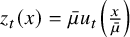 of the scaled Willmore flow
$ \bar {\mu } F_t $
 over
$ A\times \{0\} $
 satisfy v), that is,

Step 5.3: Append final correcting homotopies.
During this regular homotopy, we reparametrize
$ \bar \mu F_t $
 appropriately such that
$ \bar \mu F_t|_{C_i} $
 is a graph over
$ A\times \{0\} $
 for iv) to hold. Finally, we append a scaling regular homotopy that brings the round sphere to any given radius
$ R\geq \Lambda $
 . It is now tangent to the
$ x $
 -
$ y $
 -plane and centered at
$ (0,0,R) $
 (type
$ \beta $
 ) or
$ (0,0,-R) $
 (type
$ \alpha $
 ). Then, we append a translation that shifts the center of the sphere from
$ \pm (0,0,R) $
 to
$ \pm \left (0,0,\sqrt {R^2-1}\right ) $
 . The translation brings the sphere into the form as described in Definition 2.3. In the case of the sphere lying entirely above the horizontal plane (type
$ \beta $
 ), it is now tangent to the catenoid
$ H^c_1 $
 in the unit circle
$ \mathbb {S}^1 \times \{0\} $
 . By equation (2.10), these two steps do not violate v). Reversing the shift of all surfaces by
$ -\left (0,0,\lambda ^{-1}\text{ arccosh}(\lambda )\right ) $
 , we observe that the sphere satisfies vi).
Proof of Theorem 1.2.
Fix
$ \Lambda ,\delta _0 $
 from Lemma 2.4 i) and
$ \delta \in (0,\delta _0) $
 sufficiently small such that
$ \varepsilon := 4\pi - W_\beta (\Lambda ,\Lambda ,\delta ) $
 is positive (see Lemma 2.4 ii)). Then, choose
$ \lambda _1>\Lambda $
 sufficiently large such that
$ W_{\alpha /\beta }(\lambda ,\lambda ,\delta )< 4\pi + \varepsilon $
 for all
$ \lambda>\lambda _1 $
 (see Lemma 2.4 iii)). Apply Proposition 2.7 for
$ \delta $
 and
$ R=\lambda>\lambda _1 $
 . Let
$ H $
 be the obtained homotopy and denote
$ g_0:=H_1 $
 and
$ g^i_0:=H_1|_{S_i} \in \text {CatSph}(\lambda ,\lambda ,\delta ) $
 ,
$ i=1,2 $
 . If
$ g^1_0,g^2_0 $
 are both catenoid spheres of type
$ \alpha $
 , then
$ g_0\in J $
 and we are done. We may now assume that
$ g^1_0 $
 is a catenoid sphere of type
$ \beta $
 . We deform
$ g^1_0 $
 by a homotopy of catenoid spheres
$ g^1_t := \lambda _tf_{\lambda _t} $
 with
$ f_{\lambda _t}\in \text {CatSph}_\beta (\lambda _t,\lambda _t,\delta ) $
 and

By Lemma 2.4 and
$ \lambda>\Lambda $
 and
$\delta <\delta _0 $
 , this is a regular homotopy of decreasing Willmore energy to an immersion
$ g^1_1\in \text {CatSph}_\beta (\Lambda ,\Lambda ,\delta ) $
 of Willmore energy

This regular homotopy leaves the center piece of the catenoid fixed at all times and thus naturally extends to a regular homotopy
$ g_t $
 that is equal to
$ g^1_t $
 on
$ S_1 $
 and
$ g^2_0 $
 on
$ S_2 $
 . We conclude

Therefore, by Theorem A, the Willmore flow with initial surface
$ g_1 $
 yields the last part of the desired homotopy to a round sphere.
The homotopy
$ f_{\lambda _t} $
 from the proof of Theorem 1.2 for
$ \lambda _t = 8,5,2 $
 .

Figure 9 Long description
The figure consists of three panels arranged horizontally, each featuring a blue curve on a two-dimensional coordinate system with a horizontal x-axis and a vertical y-axis.
* In the left panel, a large blue circle is centered on the y-axis, resting just above the x-axis. The circle is nearly closed, with two small red segments curving inward toward the origin from the points labeled minus 1 and 1 on the x-axis.
* In the middle panel, the blue circle has decreased in diameter. It remains centered on the y-axis, but its overall scale is smaller relative to the axes. The red segments at the base, near minus 1 and 1, show a more pronounced inward curvature toward the origin.
* In the right panel, the blue shape has shrunk significantly into a small loop. The gap between the endpoints at minus 1 and 1 on the x-axis is wider relative to the size of the loop, and the red segments curve sharply downward and inward toward the origin, illustrating the homotopy J sub lambda t as lambda t changes from 8 to 5 to 2.
We conclude the section with some observations about the family
$ J $
 defined in Definition 1.1.
Lemma 2.8. Let
$ \omega \in (8\pi ,12\pi ] $
 . There exists
$ j\in J $
 with
$ W(j)<\omega $
 such that for all
$ f\in I(\omega )\, \cap \, J $
 , there exists a regular homotopy in
$ I(\omega ) $
 from
$ f $
 to
$ j $
 or
$ -j $
 .
Proof. Fix
$ \Lambda>0 $
 from Lemma 2.4 iii). Then, we choose
$ \delta \in \left (0,\frac 12\right ) $
 and
$ \lambda _1 \geq \Lambda $
 such that

for all
$ \lambda \geq \lambda _1 $
 . Let
$ j $
 be a smoothly immersed sphere such that on each hemisphere
$ S_i $
 it is a catenoid sphere
$ j|_{S_i}\in \text {CatSph}_\alpha (\lambda _1,\lambda _1,\delta ) $
 with outer normal on the spherical parts. It has Willmore energy

Now, for given
$ f\in I(\omega )\, \cap \, J $
 , we apply Proposition 2.7 for
$ \delta $
 and
$ \lambda =R>\lambda _1 $
 to obtain a regular homotopy to some
$ i\in \text {Imm}(\mathbb {S}^2,\mathbb {R}^3) $
 with hemispheres
$ i|_{S_i}\in \text {CatSph}_\alpha (\lambda ,\lambda ,\delta ) $
 . Type
$ \beta $
 cannot occur by Theorem D. We concatenate the regular homotopy that deforms each hemisphere by
$ t\mapsto i_t|_{S_i}\in \text {CatSph}(\lambda -t,\lambda -t,\delta ) $
 ,
$ t\in [0,\lambda -\lambda _1] $
 . By equation (2.15), we have
$ W(i_t)<\omega $
 for all
$ t\in [0,1] $
 . The obtained surface has either outer or inner normal on the spherical parts and thus can be joined to
$ j $
 or
$ -j $
 by reparametrizing homotopies.
Remark 2.9. There exists a sequence of immersions
$ j_n\in J $
 with
$ W(j_n)\to 8\pi $
 . This follows from Lemma 2.8 but also already from [Reference Blatt6, Section 5]. For
$ j\in J $
 , we have
$ W(j)\geq 8\pi $
 by the Li–Yau inequality. We even have
$ W(j)>8\pi $
 ; otherwise, the Willmore flow would yield some
$ j_t\in J $
 with
$ W(j_t)<8\pi $
 since
$ j $
 is not a critical point. We conclude that the minimal Willmore energy
$ \inf _{j\in J}W(j) = 8\pi $
 is not assumed within the family
$ J $
 .
2.4 Partial global classification of singularities below
$ 16\pi $

If we replace the energy bound of
$ 12\pi $
 by
$ 16\pi $
 , we also have to consider the possibility of catenoid, trinoid and Enneper singularities [Reference Lamm and Nguyen33]. Here, trinoid refers to any complete genus zero minimal surface of total curvature
$ -8\pi $
 with three ends, as classified in [Reference López38, Theorem 3]. These have either two catenoid ends and one planar end or three catenoid ends which can have varying orientations, neck sizes and axes (with some restrictions, cf. [Reference Kusner26, Reference Pérez55]).
The approach of the previous section capitalizes on the fact that the minimal surface that models the singularity – the catenoid – has more than one end. This allowed us to divide the remaining surface around the blow-up region into parts of smaller Willmore energy. This can be applied to trinoids as well. Enneper’s surface, however, has only one end and would require an entirely different method and is therefore excluded in the following partial classification.
The construction of catenoid spheres in Section 2.2 can be generalized to include not only catenoids but also asymptotic catenoid ends and planar ends. Hence, planar ends can be connected to a round sphere, and catenoid ends can have a connection to a round sphere of type
$ \alpha $
 or
$ \beta $
 . This leads to the following additional cases.
Proposition 2.10. Let
$ f:\mathbb{S}^2 \to \mathbb{R}^3 $
 be a smooth immersion with Willmore energy less than
$ 16\pi $
 . If
$ f $
 does not develop a singularity of Enneper type (see Theorem E), then there exists a regular homotopy
$ H:\mathbb {S}^2\times [0,1]\to \mathbb {R}^3 $
 with
$ H_0=f $
 and
$ W(H_t)<W(f) $
 for all
$ t\in (0,1] $
 , where
$ H_1 $
 realizes one of the following models (see also Figure 10).
-
(a) A round sphere.
-
(b) A catenoid whose ends are $ \alpha $
-connected to round spheres (see Proposition 2.7). -
(c) Two catenoids whose four ends are each $ \alpha $
-connected to round spheres. -
(d) A trinoid whose ends are connected to round spheres and whose connections at the catenoid ends are of type $ \alpha $
.


The singularity models of Proposition 2.10. Their images in the lower half-space are displayed, and a reflection at the horizontal plane gives their full images.

Figure 10 Long description
The diagram consists of four panels labeled a, b, c, and d arranged horizontally.
* Panel a shows a single blue and purple shaded hemisphere resting on its flat circular base.
* Panel b shows two spherical forms joined at a central point. The lower form is a hemisphere, and the upper form is a sphere with a small conical indentation at the point of contact.
* Panel c shows three spherical forms stacked vertically. The bottom is a hemisphere, the middle is a full sphere, and the top is a sphere. Each junction point features a small orange-tinted conical singularity where the surfaces meet.
* Panel d shows two separate clusters. The left cluster consists of three spheres joined at a single central point. The right cluster consists of four spheres joined at a single central point. Each cluster features the same orange-tinted conical indentations at the mutual intersection points.
Proof. We repeat many arguments of the proof of Proposition 2.7 and Theorem 1.2 without going into detail. If the Willmore flow with initial surface
$ f $
 does not converge to a round sphere, it develops a singularity whose blow-up is either a catenoid, a trinoid, or Enneper’s surface (see Theorem E). The latter was ruled out by assumption.
Trinoid case:
Analogously to the catenoid case in Proposition 2.7, each of the three disks that close up the trinoid has Willmore energy less than
$ 8\pi $
 , and with the same gluing procedure, we arrive at a trinoid whose ends are
$ \alpha $
 -connected or
$ \beta $
 -connected to round spheres. Note that Lemma 2.4 uses the asymptotics of the catenoid and thus equally applies to catenoid ends of the trinoid. So, if one of the connections at a catenoid end is of type
$ \beta $
 , we employ Lemma 2.4 as in the proof of Theorem 1.2 to arrive at an immersion of Willmore energy less than
$ 12\pi $
 from which we apply Proposition 2.7 to obtain the case (a) or (b). But if all are of type
$ \alpha $
 , we arrive at (d).
Catenoid case:
The disks that close up a catenoid singularity now each have Willmore energy less than
$ 12\pi $
 , but only one of them can have Willmore energy larger than
$ 8\pi $
 . For this part, we proceed as in the proof of Proposition 2.7, but instead of using the Willmore flow to a round sphere to construct the homotopy
$ H^1 $
 , we use the regular homotopy obtained from Proposition 2.7 to one of the cases (a) or (b). In the former case, the remaining proof carries through to yield (a) or (b) for the whole surface, whereas in the latter case we obtain a catenoid piece that is attached to a sphere and to a surface of type (b). Both connections can be of either type
$ \alpha $
 or type
$ \beta $
 . If one of them is of type
$ \beta $
 , we employ Lemma 2.4 to get below an energy of
$ 12\pi $
 and apply Proposition 2.7 again. But if both connections are of type
$ \alpha $
 , we arrive at a surface described in (c).
We outline a potential notion of “Willmore flow with surgery” for spheres with energy at most
$ 16\pi $
 .
Remark 2.11. Whenever the Willmore flow with initial energy at most
$ 12\pi $
 does not converge, we replace the catenoid by two flat disks. The convergence of the two resulting Willmore flows of spheres is automatically obtained by Theorem A [Reference Kuwert and Schätzle31] for initial energies at most
$ 8\pi $
 (see the proof of Proposition 2.7). Hence, with this “surgery” we obtain convergence for all initial surfaces with energy at most
$ 12\pi $
 to either one or two round spheres. However, it is not clear whether this is a “canonical” surgery or whether there exist other ways of flowing “through” a catenoid singularity with just one sphere. Compare this to the setting of tori of revolution, where the authors of [Reference Dall’Acqua, Müller, Rupp and Schlierf12] propose a way of flowing “through” singularities of certain Willmore flows with a change of topology from torus to sphere. The discussion above for Willmore energy at most
$ 16\pi $
 yields the following.
For smooth immersions
$ f_0:\mathbb {S}^2\to \mathbb {R}^3 $
 with
$ W(f_0)\leq 16\pi $
 , a notion of “Willmore flow with surgery” with initial surface
$ f_0 $
 either has an Enneper-type singularity or converges to one, two or three round spheres.
A Appendix
Corollary 1.3. For every regular homotopy
$ H:\mathbb {S}^2\times [0,1] \to \mathbb {R}^3$
 from some
$ j\in J $
 to an embedded sphere, there exists a time
$ t\in [0,1] $
 with
$ W(H_t)>12\pi $
 .
Proof. By the Li–Yau inequality, it follows immediately that there exists a time
$ t\in [0,1] $
 with
$ W(H_t)\geq 12\pi $
 . But actually a strict inequality holds, since [Reference Seidel62] implies that there must be an immersion
$ H_t $
 with a generic triple point; in particular, all immersions in a
$ C^\infty $
 -neighborhood of that immersion have triple points. Thus, any Willmore flow started in
$ H_t $
 must still have energy at least
$ 12\pi $
 after some time
$ \varepsilon>0 $
 . And since there are no critical points at
$ 12\pi $
 , it follows that
$ W(H_t)>12\pi $
 .
Proposition 1.10. Let
$ f:\mathbb {S}^2\to \mathbb {R}^3 $
 be a sphere of revolution whose generating curve
$ c:[0,1]\to [0,\infty )\times \mathbb {R} $
 has turning number
$ \tau \in \mathbb {Z}+\frac 12 $
 . If
$ f $
 is not a round sphere, then

Proof. First, define for
$ r_0>0 $
 ,
$ h_0\in \mathbb {R} $
 the quarter circles

Without loss of generality, we may assume
$ \tau>0 $
 . Let
$ \vartheta :[0,1]\to \mathbb {R} $
 be the lift of the tangent angle of
$ c $
 with
$ \vartheta (0)=0 $
 and

for some
$ k\in \mathbb {N} $
 . Let
$ l\in \{0,1,\dots ,k\} $
 and denote
$ c=(r,h) $
 . The mean value theorem lets us pick
$ t_l $
 to be the smallest number in
$ \vartheta ^{-1}(\{2\pi l + \frac \pi 2 \}) $
 . The tangent at
$ t_l $
 is
$ (0,1) $
 . In the following, we construct
$ C^1 $
 -curves that are composed of smooth curves connected to each other at points where their tangent is
$ (0,1) $
 . For
$ l\in \{0,1,\dots ,k-1\} $
 , consider the
$ C^1 $
 -curve
$ \gamma _l $
 obtained as the concatenation of

Now, the turning number of
$ \gamma _l $
 is
$ \frac 32 $
 . In an abuse of notation, we identify each curve segment
$ \rho $
 with the surface obtained by rotating the curve and write
$ W(\rho ) $
 for its Willmore energy. Furthermore, we can approximate piecewise smooth curves by smooth curves. They can be chosen to have Willmore energy arbitrarily close to the sum of the energies of each smooth piece. We claim

This can be deduced in two ways. First, this is due to the fact that the closed plane curve obtained from mirroring
$ \gamma $
 has turning number
$ 3 $
 and thus by Hopf’s Umlaufsatz (or Theorem of turning tangents [Reference do Carmo13]) has self-intersections. Therefore, the immersion
$ f $
 is not embedded and by the Li–Yau inequality, the claim follows. Second, the surface of revolution and the turning number are preserved under the Willmore flow [Reference Blatt6]; hence, the Willmore flow with initial surface
$ f $
 cannot converge to a round sphere and by Theorem A, the claim follows. The two quarter circles produce two round hemispheres and each contributes
$ 2\pi $
 energy to equation (A.1). Hence, we obtain

Furthermore, we construct two
$ C^1 $
 -spheres of revolution by concatenating

and

Both have Willmore energy at least
$ 4\pi $
 , where
$ 2\pi $
 is contributed by the round hemispheres. Therefore,

and we obtain in total (see Figure A1 for an example)

An example for the proof of Proposition 1.10.

Figure A1 Long description
The diagram consists of five panels, each featuring a vertical black line representing an axis of rotation, indicated by a circular arrow at the top.
* Panel 1 (Leftmost): A complex blue curve labeled c is attached to the axis. It features multiple loops and three small red tick marks indicating points of intersection or critical values.
* Panel 2: A simple semi-circular arc attached to the axis, colored half blue and half green.
* Panel 3: A curve labeled gamma sub 0 that forms a single loop before returning to the axis, colored green and blue.
* Panel 4: A curve labeled gamma sub 1 that forms a more complex loop with a self-intersection, colored green and blue.
* Panel 5 (Rightmost): A smaller semi-circular arc attached to the axis, colored green and blue.
Below the panels is a mathematical expression: W ( f ) is greater than or equal to 2 pi plus 4 pi plus 4 pi plus 2 pi. Each term in the sum corresponds to one of the panels from left to right, representing the winding number or angular contribution of each geometric component.
It remains to show the strict inequality. Assume it is an equality; then
$ f $
 is a critical point of the Willmore energy. Otherwise, the Willmore flow would yield a surface contradicting the inequality since it preserves surfaces of revolution and their turning number. By assumption,
$ f $
 is not a round sphere. By Bryant’s classification [Reference Bryant9], with
$ n:=\left (\tau + \frac 12\right )\geq 2 $
 , the immersion
$ f $
 has an
$ n $
 -tuple point at which it can be inverted to obtain a complete minimal surface with
$ n $
 embedded planar ends. But, as a surface of revolution,
$ f $
 has a full curve of
$ n $
 -tuple points and the minimal surface also has
$ n $
 -tuple points as well as density
$ n $
 at infinity. This is a contradiction to [Reference Kusner25, Theorem A].
Here, we present the computations of the Willmore energy of catenoid spheres omitted in Lemma 2.4.
Lemma A.1. There exist constants
$ \Lambda ,C>0 $
 such that for all
$ \lambda \geq \Lambda $
 and
$ \delta \in \left (0,\frac 12\right ) $

-
i) $ W^{glue}_{\alpha }(\lambda ,\delta ) \leq C\frac {1}{\delta \lambda ^2}, $
-
ii) $ W^{glue}_{\beta }(\lambda ,\delta ) \leq C \frac {\delta }{\lambda ^2}, $
-
iii) $ \partial _\lambda W^{glue}_{\beta }(\lambda ,\delta ) \geq - C \frac {\delta }{\lambda ^3}. $


Proof. For a general surface of revolution
$ f(t,\varphi ) = (r(t)\cos (\varphi ),r(t)\sin (\varphi ),h(t)) $
 where we set
$ r(t)=t $
 and
$ h:I\to \mathbb {R} $
 , we obtain formulas for its mean curvature
$ H $
 , the mean of the principal curvatures
$ \kappa _1 $
 and
$ \kappa _2 $
 , and its first fundamental form
$ G $
 . With
$ l(t):=\sqrt {1+h'(t)^2} $
 , we have

We first lay out the details of a catenoid sphere of type
$ \beta $
 and omit the index
$ \beta $
 . Let
$ \lambda>1 $
 and
$ \delta \in \left (0,\frac 12\right ) $
 . Let
$ u:(1/\lambda ,\infty )\to \mathbb {R} $
 and
$ v:[0,R)\to \mathbb {R} $
 be the graph parametrizations of the generating curves
$ (t,u(t)) $
 of the catenoid and
$ (t,v(t)) $
 of the sphere in the catenoid sphere construction, respectively (see Definition 2.3). We have the catenoid

and the sphere

In the gluing region
$ I:=[1-\delta ,1+\delta ] $
 , the generating curve
$ h:I\to \mathbb {R}^2 $
 that interpolates between the catenoid and the sphere is defined and satisfies the following.

We note that

where the last term
$ w(t):=\partial _\lambda (v(t)-u(t)) $
 is nonpositive due to the fact that
$ w(1)=0 $
 ,
$ w'(1)=0 $
 and
$ w"<0 $
 , which can be directly deduced from the explicit formulas. Furthermore, we can infer the asymptotic behavior of the explicit functions by elementary estimations, for example, we get for all
$ \lambda \geq 3 $


We gather some estimations. In the following, we write
$ A(\lambda ,\delta ,t)\lesssim B(\lambda ,\delta ,t) $
 if there exist constants
$ \Lambda>0 $
 and
$ C>0 $
 independent of
$ \lambda $
 ,
$ \delta $
 and
$ t $
 such that
$ A(\lambda ,\delta ,t)\leq C B(\lambda ,\delta ,t) $
 for all
$ \lambda \geq \Lambda $
 ,
$ \delta \in (0,\frac 12) $
 ,
$ t\in [1-\delta ,1+\delta ] $
 . Using Taylor expansion at
$ t=1 $
 with the remainder term in Lagrange form and elementary estimations as in equation (A.3), we obtain the following.

We obtain for the interpolating function using
$ \left \lvert \phi \right \rvert \leq 1 $
 ,
$ \left \lvert \phi '\right \rvert \lesssim \frac {1}{\delta } $
 and
$ \left \lvert \phi "\right \rvert \lesssim \frac {1}{\delta ^2}, $


We plug the above estimations into the formula for the gluing energy

and obtain

which is ii).
To prove i) for type
$ \alpha $
 , we note the few differences from the computations above. Let
$ u_\alpha ,v_\alpha ,h_\alpha $
 denote the corresponding catenoid, sphere and interpolating curve of the catenoid sphere of type
$ \alpha $
 . We have
$ u_\alpha =u $
 and
$ v_\alpha =-v $
 . The only situation where the opposite sign of
$ v $
 weakens the estimations is where
$ v'(1)-u'(1)=0 $
 for type
$ \beta $
 is used. This now becomes

which weakens the following estimations to

and instead of equation (A.5), we obtain

which is i).
It remains to show iii). Writing

and using equation (A.4), we obtain

We may use the fact that for functions
$ f:\mathbb {R}\to [0,\infty ) $
 ,
$ g:\mathbb {R}\to (0,\infty ) $
 with
$ g'\leq 0 $
 , we have

We have
$ \partial _\lambda h^{\prime } <0 $
 by equation (A.2), which implies
$ \partial _\lambda \left ( t \left (1+h'(t)^2\right )^{\frac 52} \right ) < 0 $
 and thus

A case distinction on the sign of
$ \partial _\lambda J(t) $
 implies with
$ t\geq \frac 12 $
 ,

We estimate further

and obtain

which is iii).
Lemma A.2. For all
$ A_{\max }>0 $
 , there exists a radius
$ r(A_{\max })>0 $
 such that all smooth immersions
$ f:\Sigma \to \mathbb {R}^3 $
 of a closed surface
$ \Sigma $
 with second fundamental form

are graphs over a ball
$ B_r(0)\subseteq T_pf$
 in the tangent space for all
$ p\in \Sigma $
 and their graph parametrizations
$ u:B_r(0)\to \mathbb {R} $
 satisfy

Proof. By [Reference Langer34, Theorem 2.4], for all
$ \alpha \in (0,1) $
 , there exists a radius
$ r(\alpha )>0 $
 such that for all immersions
$ f:\Sigma \to \mathbb {R}^3 $
 with
$ \left \lVert A\right \rVert \leq A_{\max } $
 and for all
$ p\in \Sigma $
 , the graph parametrization
$ u:B_r(0)\to \mathbb {R}^3 $
 satisfies

Together with (see, e.g., [Reference Breuning8, Proof of Lemma 2.2])

we obtain with appropriate choice of
$ \alpha $


Acknowledgments
The authors thank Karsten Große-Brauckmann, Robert Kusner and Fabian Rupp for useful discussions and helpful comments.
Competing interests
The authors have no competing interests to declare.
Financial support
The authors were partially funded by the Deutsche Forschungsgemeinschaft (DFG, German Research Foundation) under the project number MA 7559/1-2. The second author would like to thank the Hausdorff Institute (funded by the Deutsche Forschungsgemeinschaft [DFG, German Research Foundation] under Germany’s Excellence Strategy – EXC-2047/1 – 390685813) in Bonn for a welcoming and productive stay, where part of this work was completed. This work is part of the second author’s PhD thesis.


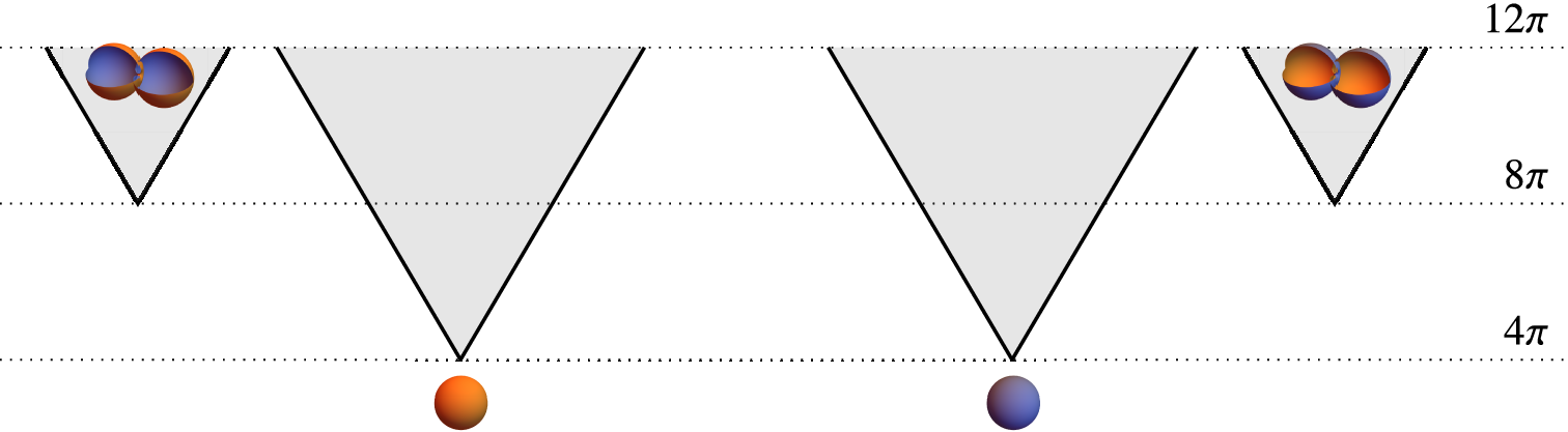


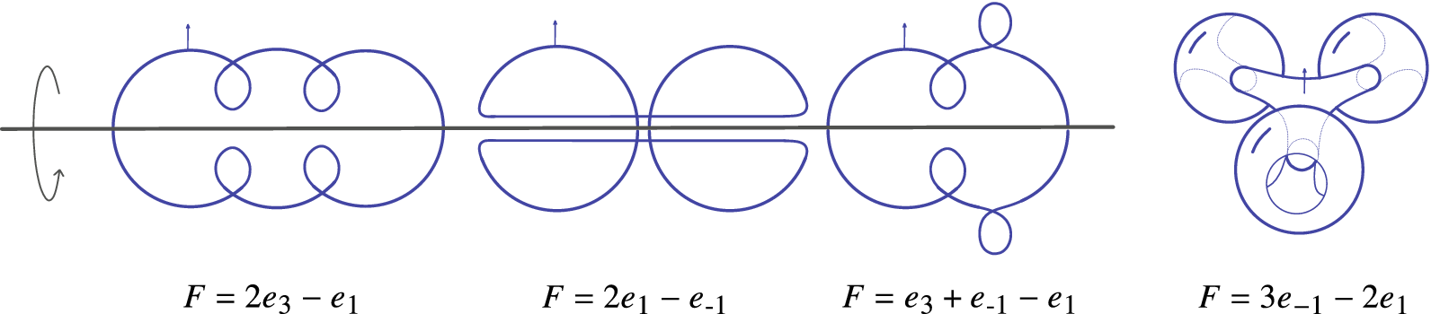

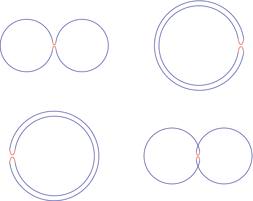
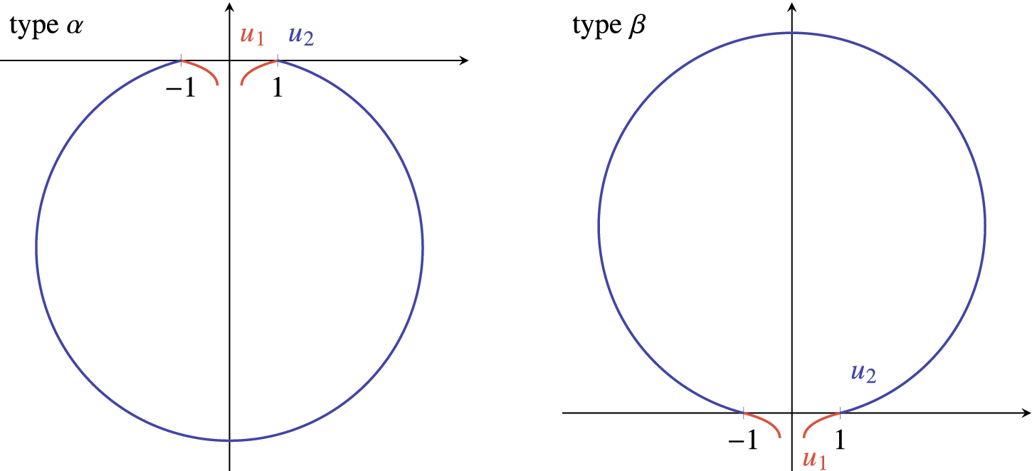


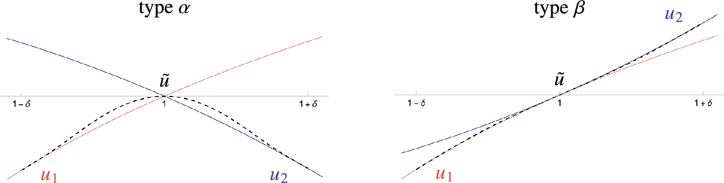

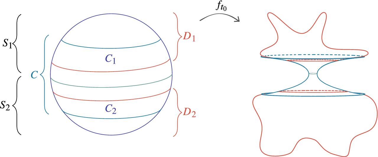


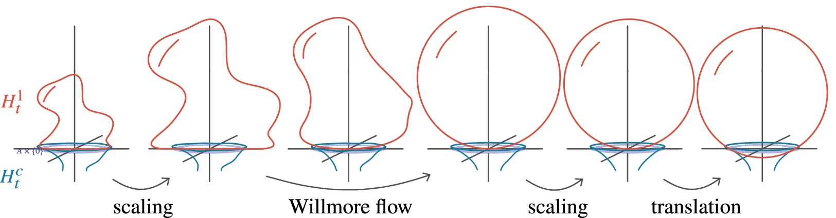

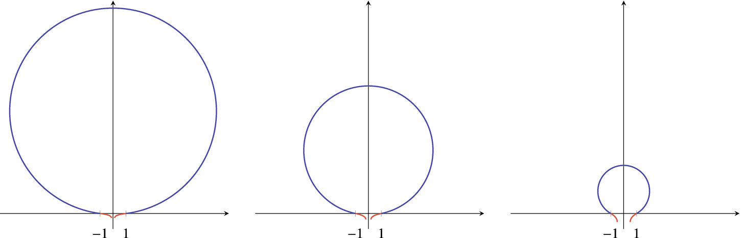


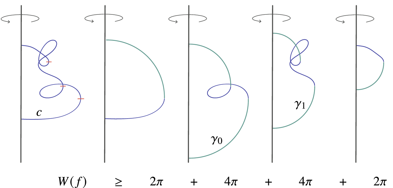

 Open access

