2. Voronoi cells with fixed nucleus

In this section we revisit the geometric properties of $A_{n}\left(x\right)$ , the cell with fixed nucleus x. We start by introducing some basic notation and terminology that will be used throughout the article. We assume that all the concerned point processes and random variables are defined on a generic probability space $\left(\Omega,\mathcal{F},\mathbb{P}\right)$ . For every set $A\in\mathcal{F}$ , $\mathbb{I}_{A}$ is the indicator function of A. For any point process $\left\{ X_{1},\cdots,X_{n}\right\} $ and any Borel set $B\subseteq\mathbb{R}^{d}$ , we define the random variable

\begin{equation*}N_{\left\{ X_{1},\cdots,X_{n}\right\} }\left(B\right): \sum_{i=1}^{n}\mathbb{I}_{\left\{ X_{i}\in B\right\} };\end{equation*}

i.e., $N_{\left\{ X_{1},\cdots,X_{n}\right\} }\left(B\right)$ is the number of points among $X_{1},\cdots,X_{n}$ that fall inside B.

Definition 2.1. Given $\Lambda>0$ , a homogeneous Poisson point process with parameter $\Lambda$ , denoted by $P_{\Lambda}$ , is a point process $\left\{ Y_{1},\cdots,Y_{n},\cdots\right\} $ with the property that for any positive integer k, any bounded and disjoint sets $B_{1},\cdots,B_{k}\subseteq\mathbb{R}^{d}$ , and any nonnegative integers $m_{1},\cdots,m_{k}$ ,

\begin{equation*}\mathbb{P}\left(N_{\left\{ Y_{1},\cdots,Y_{n},\cdots\right\} }\left(B_{i}\right)=m_{i} \quad \forall i=1,2,\cdots,k\right)=\prod_{i=1}^{k}\frac{\left(\Lambda\lambda\left(B_{i}\right)\right)^{m_{i}}}{m_{i}!}e^{-\Lambda\lambda(B_{i})}.\end{equation*}

As mentioned in Section 1, previous works on the Voronoi diagram generated by $P_{\Lambda}$ have mostly focused on the study of the ‘typical’ or ‘average’ cell as defined by the Palm calculus. This is equivalent to studying the cell with fixed nucleus $x\in\mathbb{R}^{d}$ in the Voronoi diagram generated by $\left\{ x\right\} \cup P_{\Lambda}$ . Assume that f is a probability density function on $\mathbb{R}^{d}$ and $x\in\mathbb{R}^{d}$ is such that $f\left(x\right)>0$ . For every $n\geq1$ , setting $\Lambda: nf\left(x\right)$ , we will denote by $P_{n}\left(x\right)$ the cell with nucleus x in the Voronoi diagram generated by the point process $\left\{ x\right\} \cup P_{nf\left(x\right)}$ , and by $D_{n}^{P}\left(x\right)$ the diameter of $P_{n}\left(x\right)$ . With this notation in hand, we can now precisely state the main result of this section.

Theorem 2.1. Let f be a probability density function on $\mathbb{R}^{d}$ , and let x be a Lebesgue point of f such that $f\left(x\right)>0$ . Assume that

\begin{equation*}G\,{:}\,\big\{ {convex\ polytopes\ in\ }\mathbb{R}^{d}\big\} \rightarrow\mathbb{R}\end{equation*}

is any function such that for every $n\ge1$ , $G\left(A_{n}\left(x\right)\right)$ is measurable with respect to $\sigma\left(X_{1},\cdots,X_{n}\right)$ and $G\left(P_{n}\left(x\right)\right)$ is measurable with respect to $\sigma\left(P_{nf\left(x\right)}\right)$ (e.g. $G\left(\cdot\right)$ could be the number of faces or edges of its input). Then

\begin{equation*}\lim\limits _{n\rightarrow\infty}\sup_{z\in\mathbb{R}}\left|\mathbb{P}\left(G\left(A_{n}\left(x\right)\right)\leq z\right)-\mathbb{P}\left(G\left(P_{n}\left(x\right)\right)\leq z\right)\right|=0.\end{equation*}

This result provides the link between the Voronoi diagram generated by the point process with an arbitrary density f and that generated by a homogeneous Poisson point process, which will lead to convergence in distribution for a large class of functions of the Voronoi cell $A_{n}\left(x\right)$ . The class of such functions G for which this result holds includes most tractable functions of a polytope, e.g. the volume, the surface area, the number of faces/edges, the length of each side, the locations of vertices, the location of the center of the mass, and many more, if not all, geometric properties that one might be interested in studying. In many cases, we are also interested in obtaining information on the asymptotics of the distributions of these random variables, e.g. the limit of their moments. With Theorem 2.1 and the existing results on the Voronoi diagrams generated by homogeneous Poisson point processes in hand, this task reduces to establishing proper integrability of the concerned random variable for both $A_{n}\left(x\right)$ and $P_{n}\left(x\right)$ . One demonstration of how this can be done is given in Proposition 2.1, where the expected number of edges of $A_{n}\left(x\right)$ and $P_{n}\left(x\right)$ is studied in 2D. We expect that similar arguments to the ones applied there can be used to derive the convergence of other random variables of interest, as well as to study other geometric parameters.

Before proving Theorem 2.1, we first present two technical tools that will be used in this proof as well as the proofs of other results in this article. The first tool is the following version of Chernoff’s bound, whose proof can be found in, e.g., Biau and Devroye [Reference Biau and Devroye2] (Theorem 20.19).

Lemma 2.1. (Chernoff’s bound [Reference Chernoff6]). Let Z be a random variable with the Bin $\left(n,p\right)$ distribution with parameters n and $p\in(0,1)$ . For every $t>0$ , set

\begin{equation*}\phi\left(t\right): t-np-t\ln\left(\frac{t}{np}\right)\!.\end{equation*}

Then

\begin{align*}\mathbb{P}\left(Z\geq t\right)&\leq e^{\phi\left(t\right)} \quad for\ t\geq np, and \\ \mathbb{P}\left(Z\leq t\right)&\leq e^{\phi\left(t\right)} \quad for\ 0<t\leq np.\end{align*}

The second tool we will use is the following estimate on $D_{n}^{A}\left(x\right)$ and $D_{n}^{P}\left(x\right)$ .

Lemma 2.2. Following the notation introduced above, we have that there exist universal constants $c_{1},c_{2}>0$ such that for every $t>0$ ,

\begin{equation*}\limsup\limits _{n\rightarrow\infty}\mathbb{P}\left(D_{n}^{A}\left(x\right)\geq tn^{-1/d}\right)\leq c_{1}e^{-c_{2}\,f\left(x\right)t^{d}}\end{equation*}

and

\begin{equation*}\limsup\limits _{n\rightarrow\infty}\mathbb{P}\left(D_{n}^{P}\left(x\right)\geq tn^{-1/d}\right)\leq c_{1}e^{-c_{2}\,f\left(x\right)t^{d}}.\end{equation*}

We again omit the proof here because the first statement is exactly Theorem 5.1 of Devroye et al. [Reference Devroye, Györfi, Lugosi and Walk7], and the second statement can be proven by only making minor adjustments to the proof of the first statement.

We are now ready to prove the main theorem of this section.

Proof of Theorem 2.1. Let f and x be as in the statement of the theorem. The main idea of the proof is that for large n, $A_{n}\left(x\right)$ is contained in a small region around x on which f is well approximated by $f\left(x\right)$ . Moreover, by choosing this region appropriately we can establish that for some constant $c>0$ the number of points among $X_{1},\cdots,X_{n}$ that fall into this region will have the distribution Bin( $n, c/n$ ), i.e., the binomial distribution with parameters n and $c/n$ , which is ‘approximately’ Poisson $\left(c\right)$ , the Poisson distribution with parameter c, when n is large. As a result, for all n sufficiently large, $A_{n}\left(x\right)$ can be approximately viewed as having arisen from a homogeneous Poisson point process. To make this statement precise, we observe that Lemma 2.2 implies that for arbitrary $\epsilon>0$ , there exists $t>0$ such that for all n sufficiently large,

\begin{equation*}\mathbb{P}\left(D_{n}^{A}\left(x\right)>tn^{-1/d}\right)<\epsilon \quad \text{ and } \quad \mathbb{P}\left(D_{n}^{P}\left(x\right)>tn^{-1/d}\right)<\epsilon.\end{equation*}

Therefore, with t chosen and fixed, we apply Lemma 2.1 to get that for any $\phi>0$ and for all n sufficiently large,

\begin{equation*}\left|\frac{\mu_{f}\left(B_{x,2tn^{-1/d}}\right)}{\lambda\left(B_{x,2tn^{-1/d}}\right)}-f\left(x\right)\right|\leq\phi f\left(x\right)\!.\end{equation*}

We write $\lambda_{0}: \lambda\left(B_{0,1}\right)$ to simplify the notation. It follows from above that

(3) \begin{equation}\frac{\left(1-\phi\right)\lambda_{0}\,f\left(x\right)2^{d}t^{d}}{n}\leq\mu_{f}\left(B_{x,2tn^{-1/d}}\right)\leq\frac{\left(1+\phi\right)\lambda_{0}\,f\left(x\right)2^{d}t^{d}}{n}.\end{equation}

Recall that $N_{\left\{ X_{1},\cdots,X_{n}\right\} }\left(B\right)$ is the number of points among $X_{1},\cdots,X_{n}$ that lie in a set $B\subseteq\mathbb{R}^{d}$ . Choose $M>0$ large such that for all n sufficiently large,

\begin{equation*}\begin{split} & \mathbb{P}\left(N_{\left\{ X_{1},\cdots,X_{n}\right\} }\left(B_{x,2tn^{-1/d}}\right)>M\right)\\[4pt] = & \, \text{Bin}\left(n,\mu_{f}\left(B_{x,2tn^{-1/d}}\right)\right)\left(\left(M,\infty\right)\right)\\[4pt] \leq & \exp\left[M-\left(1-\phi\right)\lambda_{0}f\left(x\right)2^{d}t^{d}-M\ln M+M\ln\left(\left(1+\phi\right)\lambda_{0}f\left(x\right)2^{d}t^{d}\right)\right],\end{split}\end{equation*}

where the last inequality is due to (3) and, again, Lemma 2.1. Clearly, by choosing M large, we can make the expression above smaller than $\epsilon$ . So, we obtain that

(4) \begin{align} & \mathbb{P}\left(G\left(A_{n}\left(x\right)\right)\leq z\right)-\mathbb{P}\left(G\left(A_{n}\left(x\right)\right)\leq z,D_{n}^{A}\left(x\right)\leq tn^{-1/d},N_{\left\{ X_{1},\cdots,X_{n}\right\} }\left(B_{x,2tn^{-1/d}}\right)\leq M\right)\nonumber\\ & \quad\leq \mathbb{P}\left(D_{n}^{A}\left(x\right)>tn^{-1/d}\right)+\mathbb{P}\left(N_{\left\{ X_{1},\cdots,X_{n}\right\} }\left(B_{x,2tn^{-1/d}}\right)>M\right)\leq2\epsilon.\end{align}

Now, observe that

(5) \begin{align} & \mathbb{P}\left(G\left(A_{n}\left(x\right)\right)\leq z,D_{n}^{A}(x)\leq tn^{-1/d},N_{\left\{ X_{1},\cdots,X_{n}\right\} }\left(B_{x,2tn^{-1/d}}\right)\leq M\right)\nonumber\\[4pt] & = \sum_{i=0}^{M}\mathbb{P}\left(G\left(A_{n}\left(x\right)\right)\leq z,D_{n}^{A}(x)\leq tn^{-1/d},N_{\left\{ X_{1},\cdots,X_{n}\right\} }\left(B_{x,2tn^{-1/d}}\right)=i\right)\nonumber\\[4pt] & = \sum_{i=0}^{M}\mathbb{P}\left(\left.G\left(A_{n}\left(x\right)\right)\leq z,D_{n}^{A}(x)\leq tn^{-1/d}\right|\left\{ X_{1},\cdots,X_{n}\right\} \cap B_{x,2tn^{-1/d}}=\left\{ X_{1},\cdots,X_{i}\right\} \right)\nonumber\\[4pt] &\quad \cdot\binom{n}{i}\left[\mu_{f}\left(B_{x,2tn^{-1/d}}\right)\right]^{i}\left[1-\mu_{f}\left(B_{x,2tn^{-1/d}}\right)\right]^{n-i}.\end{align}

On the other hand, for every $n\geq1$ , in the case when the Voronoi diagram is generated by the homogeneous Poisson point process $P_{nf\left(x\right)}$ , $N_{P_{nf\left(x\right)}}\left(B_{x,2tn^{-1/d}}\right)$ is just a Poisson random variable with parameter

\begin{equation*}nf\left(x\right)\lambda\left(B_{x,2tn^{-1/d}}\right)=\lambda_{0}f\left(x\right)2^{d}t^{d}\end{equation*}

which does not depend on n. Thus, by choosing M sufficiently large, we can make

\begin{equation*}\mathbb{P}\left(N_{P_{nf\left(x\right)}}\left(B_{x,2tn^{-1/d}}\right)>M\right)<\epsilon\end{equation*}

for all $n\geq1$ , and hence we also have

(6) \begin{align}\mathbb{P}\left(G\left(P_{n}\left(x\right)\right)\leq z\right)-\mathbb{P}\left(G\left(P_{n}\left(x\right)\right)\leq z,D_{n}^{P}\left(x\right)\leq tn^{-1/d},N_{P_{nf\left(x\right)}}\left(B_{x,2tn^{-1/d}}\right)\leq M\right)\leq2\epsilon.\nonumber\\ \end{align}

Further,

(7) \begin{align} & \mathbb{P}\left(G\left(P_{n}\left(x\right)\right)\leq z,D_{n}^{P}\left(x\right)\leq tn^{-1/d},N_{P_{nf\left(x\right)}}\left(B_{x,2tn^{-1/d}}\right)\leq M\right)\nonumber\\[4pt] &\quad = \sum_{i=0}^{M}\mathbb{P}\left(\left.G\left(P_{n}\left(x\right)\right)\leq z,D_{n}^{P}\left(x\right)\leq tn^{-1/d}\right|N_{P_{nf\left(x\right)}}\left(B_{x,2tn^{-1/d}}\right)=i\right)\nonumber\\[4pt] & \qquad\cdot\frac{\left[\lambda_{0}f\left(x\right)2^{d}t^{d}\right]^{i}}{i!}e^{-\lambda_{0}f\left(x\right)2^{d}t^{d}}.\end{align}

Combining (4)–(7), we conclude that in order to control

\begin{equation*}\sup_{z\in\mathbb{R}}\left|\mathbb{P}\left(G\left(A_{n}\left(x\right)\right)\leq z\right)-\mathbb{P}\left(G\left(P_{n}\left(x\right)\right)\leq z\right)\right|,\end{equation*}

it is sufficient to prove the following two facts.

Fact 1. For every $i\in\left\{ 0,\cdots,M\right\} $ ,

\begin{equation*}\lim\limits _{n\rightarrow\infty}\binom{n}{i}\left[\mu_{f}\left(B_{x,2tn^{-1/d}}\right)\right]^{i}\left[1-\mu_{f}\left(B_{x,2tn^{-1/d}}\right)\right]^{n-i}=\frac{\left[\lambda_{0}f\left(x\right)2^{d}t^{d}\right]^{i}}{i!}e^{-\lambda_{0}f\left(x\right)2^{d}t^{d}}.\end{equation*}

Fact 2. For every $i\in\left\{ 0,\cdots,M\right\} $ ,

\begin{align*} & \lim\limits _{n\rightarrow\infty}\sup_{z\in\mathbb{R}}\left|\mathbb{P}\left(\left.G\left(A_{n}\left(x\right)\right)\leq z,\ D_{n}^{A}\left(x\right)\leq tn^{-1/d}\right|\left\{ X_{1},\cdots,X_{n}\right\} \cap B_{x,2tn^{-1/d}}=\left\{ X_{1},\cdots,X_{i}\right\} \right)\right.\\[5pt] & \quad -\left.\mathbb{P}\left(\left.G\left(P_{n}\left(x\right)\right)\leq z,\ D_{n}^{P}\left(x\right)\leq tn^{-1/d}\right|N_{P_{nf\left(x\right)}}\left(B_{x,2tn^{-1/d}}\right)=i\right)\right|=0.\end{align*}

Proof of Fact 1: Fact 1 follows from a straightforward application of the Lebesgue differentiation theorem. To be specific, let $\phi>0$ be arbitrary. By (3), we have that

\begin{align*}& \limsup_{n\rightarrow\infty}\binom{n}{i}\left[\mu_{f}\left(B_{x,2tn^{-1/d}}\right)\right]^{i}\left[1-\mu_{f}\left(B_{x,2tn^{-1/d}}\right)\right]^{n-i}\\[5pt] & \leq \limsup_{n\rightarrow\infty}\binom{n}{i}\left[\frac{\left(1+\phi\right)\lambda_{0}f\left(x\right)2^{d}t^{d}}{n}\right]^{i}\left[1-\frac{\left(1-\phi\right)\lambda_{0}f\left(x\right)2^{d}t^{d}}{n}\right]^{n-i}\\[5pt] & =\frac{\left[\left(1+\phi\right)\lambda_{0}f\left(x\right)2^{d}t^{d}\right]^{i}}{i!}e^{-\left(1-\phi\right)\lambda_{0}f\left(x\right)2^{d}t^{d}},\end{align*}

and similarly,

\begin{align*}&\liminf_{n\rightarrow\infty}\binom{n}{i}\left[\mu_{f}\left(B_{x,2tn^{-1/d}}\right)\right]^{i}\left[1-\mu_{f}\left(B_{x,2tn^{-1/d}}\right)\right]^{n-i}\\[5pt] & \geq \frac{\left[\left(1-\phi\right)\lambda_{0}f\left(x\right)2^{d}t^{d}\right]^{i}}{i!}e^{-\left(1+\phi\right)\lambda_{0}f\left(x\right)2^{d}t^{d}}.\end{align*}

Since $\phi>0$ is arbitrary, we have proven Fact 1.

Proof of Fact 2: First, we observe that if $D_{n}^{A}\left(x\right)\leq tn^{-1/d}$ (or $D_{n}^{P}\left(x\right)\leq tn^{-1/d}$ ), then for every $z\in B_{x,tn^{-1/d}}$ and every $X_{i}\notin B_{x,2tn^{-1/d}}$ ,

\begin{equation*}\left\Vert z-x\right\Vert <tn^{-1/d}<\left\Vert X_{i}-x\right\Vert -\left\Vert x-z\right\Vert \leq\left\Vert X_{i}-z\right\Vert ,\end{equation*}

which means that $X_{i}$ has no effect on the forming of $A_{n}\left(x\right)$ (or $P_{n}\left(x\right)$ ). In other words, the sample points among $X_{1},\cdots,X_{n}$ that fall outside of $B_{x,2tn^{-1/d}}$ are irrelevant to the cell with nucleus x.

Next, for every $z\in\mathbb{R}$ , we define $E_{z}$ to be the collection of all sets of i points $\left\{ x_{1},\cdots,x_{i}\right\} \subseteq\mathbb{R}^{d}$ such that

1. (i) $\left\{ x_{1},\cdots,x_{i}\right\} \subseteq B_{x,2tn^{-1/d}}$ ;

2. (ii) $G\left(A_{i}^{\prime}\left(x\right)\right)\leq z$ , where $A_{i}^{\prime}\left(x\right)$ is the Voronoi cell with nucleus x generated by $\left\{ x,x_{1},\cdots,x_{i}\right\} $ ;

3. (iii) $D_{i}^{A^{\prime}}\left(x\right)\leq tn^{-1/d}$ , where $D_{i}^{A^{\prime}}\left(x\right)$ is the diameter of $A_{i}^{\prime}\left(x\right)$ .

From the observation above, we know that if $X_{1},\cdots,X_{i}$ are the only points among $X_{1},\cdots,X_{n}$ that are inside $B_{x,2tn^{-1/d}}$ , then $A_{n}\left(x\right)$ is the same as $A_{i}\left(x\right)$ when only the points $\left\{ x,X_{1},\cdots,X_{i}\right\} $ are used in generating the Voronoi diagram. Therefore, for every $z\in\mathbb{R}$ ,

\begin{align*} & \mathbb{P}\left(\left.G\left(A_{n}\left(x\right)\right)\leq z,D_{n}^{A}\left(x\right)\leq tn^{-1/d}\right|\left\{ X_{1},\cdots,X_{n}\right\} \cap B_{x,2tn^{-1/d}}=\left\{ X_{1},\cdots,X_{i}\right\} \right)\\[4pt] & =\frac{\mathbb{P}\left(\left\{ X_{1},\cdots,X_{i}\right\} \in E_{z},X_{i+1},\cdots,X_{n}\notin B_{x,2tn^{-1/d}}\right)}{\mathbb{P}\left(\left\{ X_{1},\cdots,X_{n}\right\} \cap B_{x,2tn^{-1/d}}=\left\{ X_{1},\cdots,X_{i}\right\} \right)}\\[4pt] & = \frac{\mathbb{P}\left(\left\{ X_{1},\cdots,X_{i}\right\} \in E_{z}\right)\mathbb{P}\left(X_{i+1},\cdots,X_{n}\notin B_{x,2tn^{-1/d}}\right)}{\mathbb{P}\left(X_{1},\cdots,X_{i}\in B_{x,2tn^{-1/d}}\right)\mathbb{P}\left(X_{i+1},\cdots,X_{n}\notin B_{x,2tn^{-1/d}}\right)}\\[4pt] & = \mathbb{P}\left(\left\{ X_{1},\cdots,X_{i}\right\} \in E_{z}\left|X_{1},\cdots,X_{i}\in B_{x,2tn^{-1/d}}\right.\right)\!.\end{align*}

By a similar argument as above and basic properties of homogeneous Poisson point processes, we also have that

\begin{equation*}\mathbb{P}\left(\left.G\left(P_{n}\left(x\right)\right)\leq z,D_{n}^{P}\left(x\right)\leq tn^{-1/d}\right|N_{P_{nf\left(x\right)}}\left(B_{x,2tn^{-1/d}}\right)=i\right)=\mathbb{P}\left(\left\{ U_{1},\cdots,U_{i}\right\} \in E_{z}\right)\!,\end{equation*}

where $U_{1},\cdots,U_{i}$ are i.i.d. random variables with the uniform distribution on $B_{x,2tn^{-1/d}}$ .

Finally it is easy to see that the conditional distribution of $\left\{ X_{1},\cdots,X_{i}\right\} $ , conditioning on the event that $X_{1},\cdots,X_{i}\in B_{x,2tn^{-1/d}}$ , has the probability density function

\begin{equation*}\frac{f\left(x_{1}\right)f\left(x_{2}\right)\cdots f\left(x_{i}\right)}{\left[\mu_{f}\left(B_{x,2tn^{-1/d}}\right)\right]^{i}} \quad \text{ for every }x_{1},\cdots,x_{i}\in B_{x,2tn^{-1/d}}.\end{equation*}

Thus, to prove Fact 2, it is enough for us to show that

\begin{align*} & \left|\mathbb{P}\left(\left\{ X_{1},\dots,X_{i}\right\} \in E_{z}\left|X_{1},\dots,X_{i}\in B_{x,2tn^{-1/d}}\right.\right)-\mathbb{P}\left(\left\{ U_{1},\cdots,U_{i}\right\} \in E_{z}\right)\right|\\[4pt] & \leq \idotsint_{E_{z}}\left|\prod_{j=1}^{i}\frac{f\left(x_{j}\right)}{\mu_{f}\left(B_{x,2tn^{-1/d}}\right)}-\prod_{j=1}^{i}\frac{n}{\lambda_{0}2^{d}t^{d}}\right|dx_{1}\cdots dx_{i}\\[4pt] & \leq \int_{B_{x,2tn^{-1/d}}}\cdots\int_{B_{x,2tn^{-1/d}}}\left|\prod_{j=1}^{i}\frac{f\left(x_{j}\right)}{\mu_{f}\left(B_{x,2tn^{-1/d}}\right)}-\prod_{j=1}^{i}\frac{n}{\lambda_{0}2^{d}t^{d}}\right|dx_{1}\cdots dx_{i}\\\rightarrow & 0 \quad \text{ as }n\rightarrow\infty.\end{align*}

The convergence in the last line can be verified using the Lebesgue differentiation theorem in a straightforward way. We omit the details here but present it as a lemma (Lemma A.2) in the Appendix. So, we obtain that

\begin{equation*}\lim_{n\rightarrow\infty}\sup_{z\in\mathbb{R}}\left|\mathbb{P}\left(\left\{ X_{1},\cdots,X_{i}\right\} \in E_{z}\left|X_{1},\cdots,X_{i}\in B_{x,2tn^{-1/d}}\right.\right)-\mathbb{P}\left(\left\{ U_{1},\cdots,U_{i}\right\} \in E_{z}\right)\right|=0,\end{equation*}

which concludes the proof of Fact 2, as well as the proof of Theorem 2.1.□

We now give an explicit example of how Theorem 2.1 can be used to derive a limit for the expected number of edges of $A_{n}\left(x\right)$ when $d=2$ .

Proposition 2.1. Let $d=2$ , let f be a probability density function on $\mathbb{R}^{d}$ , and let x be a Lebesgue point of f such that $f\left(x\right)>0$ . Then

\begin{equation*}\sup_{n\geq1}\mathbb{E}\Big[\left(the\ number\ of\ edges\ of\ A_{n}\left(x\right)\right)^{2}\Big]<\infty.\end{equation*}

Moreover,

\begin{equation*}\lim\limits _{n\rightarrow\infty}\mathbb{E}\left[the\ number\ of\ edges\ of\ A_{n}\left(x\right)\right]=6.\end{equation*}

Proof. We recall that the expected number of edges of $P_{n}\left(x\right)$ is equal to 6 (see, e.g., Meijering [Reference Meijering14]). Also, by a direct corollary of Theorem 5.3 of Heinrich and Muche [Reference Heinrich and Muche13], we have that for every $n\geq1$ ,

\begin{equation*}\mathbb{E}\left[\left(\text{the number of edges of }P_{n}\left(x\right)\right)^{2}\right]=\mathbb{E}\left[\left(\text{the number of edges of }P_{1}\left(x\right)\right)^{2}\right]<\infty.\end{equation*}

Now assume that the first statement of Proposition 2.1 holds, i.e., the second moment of the number of edges of $A_{n}\left(x\right)$ is bounded in n. By taking $G\left(\cdot\right)$ to be the number of edges of its input in Theorem 2.1, one can easily check that

\begin{equation*}\lim\limits _{n\rightarrow\infty}\mathbb{E}\left[\text{the number of edges of }A_{n}\left(x\right)\right]=\lim\limits _{n\rightarrow\infty}\mathbb{E}\left[\text{the number of edges of }P_{n}\left(x\right)\right]=6.\end{equation*}

Therefore, we only need to focus on proving the first statement of Proposition 2.1.

To this end, we first observe that since with probability 1 every vertex of $A_{n}\left(x\right)$ has degree 3 in the Voronoi diagram, we have that every vertex of $A_{n}\left(x\right)$ is also a vertex of a unique pair of Voronoi cells adjacent to $A_{n}\left(x\right)$ . For all $i,j\in\left\{ 1,\cdots,n\right\} $ such that $i\neq j$ , let $E_{i,j}$ denote the event that $A_{n}\left(X_{i}\right)$ , $A_{n}\left(X_{j}\right)$ , and $A_{n}\left(x\right)$ share a vertex. Then we have that

\begin{equation*}\begin{split}\mathbb{E}\left[\left(\text{the number of edges of }A_{n}\left(x\right)\right)^{2}\right] & =\mathbb{E}\left[\left(\text{the number of vertices of }A_{n}\left(x\right)\right)^{2}\right]\\[4pt] & =\mathbb{E}\left[\left(\sum_{i,j\in\{1,\cdots,n\},\ i<j}\mathbb{I}_{E_{i,j}}\right)^{2}\right].\end{split}\end{equation*}

Let i, j, k, and l be four distinct integers in $\left\{ 1,\cdots,n\right\} $ . There are three types of terms resulting from expanding the expectation above:

1. 1. There are $n\left(n-1\right)/2=\mathcal{O}\left(n^{2}\right)$ terms of the form

   \begin{equation*}\mathbb{E}\left[\left(\mathbb{I}_{E_{i,j}}\right)^{2}\right]=\mathbb{P}\left(E_{i,j}\right)\!.\end{equation*}

2. 2. There are $n\left(n-1\right)\left(n-2\right)=\mathcal{O}\left(n^{3}\right)$ terms of the form

   \begin{equation*}\mathbb{E}\left[\mathbb{I}_{E_{i,j}}\mathbb{I}_{E_{i,k}}\right]=\mathbb{P}\left(E_{i,j}\cap E_{i,k}\right)\!.\end{equation*}

3. 3. There are $n\left(n-1\right)\left(n-2\right)\left(n-3\right)/4=\mathcal{O}\left(n^{4}\right)$ terms of the form

   \begin{equation*}\mathbb{E}\left[\mathbb{I}_{E_{i,j}}\mathbb{I}_{E_{l,k}}\right]=\mathbb{P}\left(E_{i,j}\cap E_{l,k}\right)\!.\end{equation*}

In particular, since $X_{1},\cdots,X_{n}$ are all identically distributed, it is enough to show that the following three quantities are finite:

\begin{equation*}\sup_{n\geq2}n^{2}\mathbb{P}\left(E_{1,2}\right)\!, \quad \sup_{n\geq3}n^{3}\mathbb{P}\left(E_{1,2}\cap E_{1,3}\right)\!, \quad \text{and} \quad \sup_{n\geq4}n^{4}\mathbb{P}\left(E_{1,2}\cap E_{3,4}\right)\!.\end{equation*}

We will only give an explicit proof that the last quantity is finite. The finiteness of the first two quantities can be shown in an identical manner.

For any three points $w,u,v\in\mathbb{R}^{2}$ that do not lie on the same line, let $c\left(w,u,v\right)$ denote the circumcenter of w, u and v. Observe that $E_{i,j}$ is equivalent to the event that

\begin{equation*}\left\Vert X_{k}-c\left(x,X_{i},X_{j}\right)\right\Vert \geq\left\Vert x-c\left(x,X_{i},X_{j}\right)\right\Vert \quad \forall k\in\left\{ 1,\cdots,n\right\} \backslash\left\{ i,j\right\} .\end{equation*}

To see this, notice that the vertex shared by $A_{n}\left(x\right)$ , $A_{n}\left(X_{i}\right)$ , and $A_{n}\left(X_{j}\right)$ is just $c\left(x,X_{i},X_{j}\right)$ , and $c\left(x,X_{i},X_{j}\right)$ is in all three of $A_{n}\left(x\right)$ , $A_{n}\left(X_{i}\right)$ , and $A_{n}\left(X_{j}\right)$ if and only if $c\left(x,X_{i},X_{j}\right)$ is not strictly closer to any of the other points among $X_{1},\cdots,X_{n}$ . Therefore, we have that

\begin{align*} & \mathbb{P}\left(E_{1,2}\cap E_{3,4}\right)\\[4pt] & \le \mathbb{P}\left(\bigcap_{k=5}^{n}\left\{ \left\Vert X_{k}-c\left(x,X_{1},X_{2}\right)\right\Vert \geq\left\Vert x-c\left(x,X_{1},X_{2}\right)\right\Vert ,\left\Vert X_{k}-c\left(x,X_{3},X_{4}\right)\right\Vert\right.\right.\\[4pt] & \qquad\left.\geq\left\Vert x-c\left(x,X_{3},X_{4}\right)\right\Vert \right\} \Bigg)\\[4pt] & = \mathbb{E}\left[\left(1-\mu_{f}\left(B_{c(x,X_{1},X_{2}),\left\Vert x-c\left(x,X_{1},X_{2}\right)\right\Vert }\cup B_{c(x,X_{3},X_{4}),\left\Vert x-c\left(x,X_{3},X_{4}\right)\right\Vert }\right)\right)^{n-4}\right].\end{align*}

We claim that in order to prove that

\begin{equation*}\sup_{n\geq4}n^{4}\mathbb{E}\left[\left(1-\mu_{f}\left(B_{c(x,X_{1},X_{2}),\left\Vert x-c\left(x,X_{1},X_{2}\right)\right\Vert }\cup B_{c(x,X_{3},X_{4}),\left\Vert x-c\left(x,X_{3},X_{4}\right)\right\Vert }\right)\right)^{n-4}\right]<\infty,\end{equation*}

it is enough to show that

(8) \begin{equation}\limsup_{z\rightarrow0}z^{-4}\mathbb{P}\left(\mu_{f}\left(B_{c(x,X_{1},X_{2}),\left\Vert x-c\left(x,X_{1},X_{2}\right)\right\Vert }\cup B_{c(x,X_{3},X_{4}),\left\Vert x-c\left(x,X_{3},X_{4}\right)\right\Vert }\right)\leq z\right)<\infty.\end{equation}

Suppose (8) holds. Then there exist $M>0$ and $\eta>0$ such that for every $z\in\left(0,\eta\right)$ ,

\begin{equation*}\mathbb{P}\left(\mu_{f}\left(B_{c(x,X_{1},X_{2}),\left\Vert x-c\left(x,X_{1},X_{2}\right)\right\Vert }\cup B_{c(x,X_{3},X_{4}),\left\Vert x-c\left(x,X_{3},X_{4}\right)\right\Vert }\right)\leq z\right)\leq z^{4}M.\end{equation*}

Therefore, we have that

\begin{align*} & n^{4}\mathbb{E}\left[\left(1-\mu_{f}\left(B_{c(x,X_{1},X_{2}),\left\Vert x-c\left(x,X_{1},X_{2}\right)\right\Vert }\cup B_{c(x,X_{3},X_{4}),\left\Vert x-c\left(x,X_{3},X_{4}\right)\right\Vert }\right)\right)^{n-4}\right]\\ &\!\!\quad = n^{4}\left(n-4\right)\int_{0}^{1}\left(1-z\right)^{n-5}\mathbb{P}\left(\mu_{f}\left(B_{c(x,X_{1},X_{2}),\left\Vert x-c\left(x,X_{1},X_{2}\right)\right\Vert }\cup B_{c(x,X_{3},X_{4}),\left\Vert x-c\left(x,X_{3},X_{4}\right)\right\Vert }\right)\leq z\right)dz\\ &\!\!\quad \leq n^{4}\left(n-4\right)\int_{0}^{\eta}\left(1-z\right)^{n-5}\mathbb{P}\left(\mu_{f}\left(B_{c(x,X_{1},X_{2}),\left\Vert x-c\left(x,X_{1},X_{2}\right)\right\Vert }\cup B_{c(x,X_{3},X_{4}),\left\Vert x-c\left(x,X_{3},X_{4}\right)\right\Vert }\right)\leq z\right)dz\\ &\!\!\qquad +n^{4}\left(n-4\right)\int_{\eta}^{1}\left(1-z\right)^{n-5}dz\\ &\!\!\quad \leq Mn^{4}\left(n-4\right)\int_{0}^{\eta}\left(1-z\right)^{n-5}z^{4}dz+n^{4}\left(1-\eta\right)^{n-4}\\ &\!\!\quad = \frac{4!Mn^{3}}{\left(n-1\right)\left(n-2\right)\left(n-3\right)}+\mathcal{O}\left(n^{4}\left(1-\eta\right)^{n-4}\right)\!,\end{align*}

which is clearly bounded in n. Now we will focus on proving (8).

By the generalized Lebesgue differentiation theorem (see, e.g., Theorem 5.3 of Devroye and Lugosi [Reference Devroye and Lugosi9]), there exists $\delta>0$ such that for every $y\in B_{x,\delta}$ ,

(9) \begin{equation}\left|\frac{\mu_{f}\left(B_{x,\left\Vert y-x\right\Vert }\right)}{\lambda\left(B_{x,\left\Vert y-x\right\Vert }\right)}-f\left(x\right)\right|\leq\frac{1}{2}\,f\left(x\right) \quad \text{and} \quad \left|\frac{\mu_{f}\left(B_{y,\left\Vert y-x\right\Vert }\right)}{\lambda\left(B_{y,\left\Vert y-x\right\Vert }\right)}-f\left(x\right)\right|\leq\frac{1}{2}\,f(x).\end{equation}

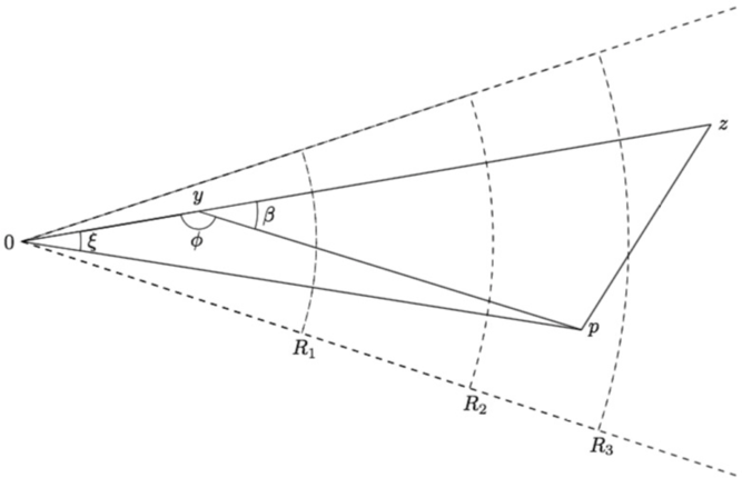
We claim that if $\left\Vert x-c\left(x,X_{1},X_{2}\right)\right\Vert >\delta/2$ , then it must be that

\begin{equation*}\mu_{f}\left(B_{c(x,X_{1},X_{2}),\left\Vert x-c\left(x,X_{1},X_{2}\right)\right\Vert }\right)\geq\frac{1}{8}\,f\left(x\right)\pi\delta^{2}.\end{equation*}

To see this let $c^{*}$ be the point on the line segment connecting x and $c\left(x,X_{1},X_{2}\right)$ such that $\left\Vert x-c^{*}\right\Vert =\delta/2$ . Then $B_{c^{*},\delta/2}\subseteq B_{c(x,X_{1},X_{2}),\left\Vert x-c\left(x,X_{1},X_{2}\right)\right\Vert }$ , as shown in Figure 1.

Figure 1:

$A_{n}\left(x\right)$ , $A_{n}\left(X_{1}\right)$ , and $A_{n}\left(X_{2}\right)$ sharing a vertex $c\left(x,X_{1},X_{2}\right)$ .

By (9), we have that

\begin{equation*}\mu_{f}\left(B_{c(x,X_{1},X_{2}),\left\Vert x-c\left(x,X_{1},X_{2}\right)\right\Vert }\right)\geq\mu_{f}\left(B_{c^{*},\delta/2}\right)\geq\frac{1}{2}\,f\left(x\right)\lambda(B_{c^{*},\delta/2})=\frac{1}{8}\,f\left(x\right)\pi\delta^{2},\end{equation*}

which proves the claim. Now, observe that it is also clear that

\begin{equation*}\frac{1}{2}\left\Vert x-X_{1}\right\Vert \leq\left\Vert x-c\left(x,X_{1},X_{2}\right)\right\Vert \text{ and }\frac{1}{2}\left\Vert x-X_{2}\right\Vert \leq\left\Vert x-c\left(x,X_{1},X_{2}\right)\right\Vert .\end{equation*}

Therefore,

\begin{align*}\mu_{f}\left(B_{c(x,X_{1},X_{2}),\left\Vert x-c\left(x,X_{1},X_{2}\right)\right\Vert }\right)<\frac{1}{8}\,f\left(x\right)\pi\delta^{2} & \Rightarrow\left\Vert x-c\left(x,X_{1},X_{2}\right)\right\Vert \leq\frac{\delta}{2}\\ & \Rightarrow\left\Vert x-X_{1}\right\Vert \leq\delta\text{ and }\left\Vert x-X_{2}\right\Vert \leq\delta,\end{align*}

and similarly

\begin{align*} & \mu_{f}\left(B_{c(x,X_{3},X_{4}),\left\Vert x-c\left(x,X_{3},X_{4}\right)\right\Vert }\right)<\frac{1}{8}\,f\left(x\right)\pi\delta^{2}\\ & \Rightarrow\left\Vert x-c\left(x,X_{3},X_{4}\right)\right\Vert \leq\frac{\delta}{2},\;\left\Vert x-X_{3}\right\Vert \leq\delta\text{ and }\left\Vert x-X_{4}\right\Vert \leq\delta.\end{align*}

Let E be the set defined by

\begin{equation*}\begin{array}{c}\left\{ \left\Vert x-c\left(x,X_{1},X_{2}\right)\right\Vert <\frac{\delta}{2},\left\Vert x-X_{1}\right\Vert \leq\delta,\left\Vert x-X_{2}\right\Vert \leq\delta\right\} \\[4pt] \bigcap\left\{ \left\Vert x-c\left(x,X_{3},X_{4}\right)\right\Vert \leq\frac{\delta}{2},\left\Vert x-X_{3}\right\Vert \leq\delta,\left\Vert x-X_{4}\right\Vert \leq\delta\right\} .\end{array}\end{equation*}

Finally, observe that, by (9), for every $y\in B_{x,\delta}$ ,

\begin{equation*}\mu_{f}\left(B_{x,\left\Vert y-x\right\Vert }\right)\leq\frac{3}{2}\,f\left(x\right)\lambda\left(B_{x,\left\Vert y-x\right\Vert }\right)=\frac{3}{2}\,f\left(x\right)\lambda\left(B_{y,\left\Vert y-x\right\Vert }\right)\leq3\mu_{f}\left(B_{y,\left\Vert y-x\right\Vert }\right)\!,\end{equation*}

and similarly,

\begin{equation*}\mu_{f}\left(B_{x,\left\Vert y-x\right\Vert }\right)\leq\frac{3}{2}\,f\left(x\right)\lambda\left(B_{x,\left\Vert y-x\right\Vert }\right)=6f\left(x\right)\lambda\left(B_{x,\left\Vert y-x\right\Vert /2}\right)\leq12\mu_{f}\left(B_{x,\left\Vert y-x\right\Vert /2}\right)\!.\end{equation*}

Thus, we have that for all $z<\frac{1}{8}\,f\left(x\right)\pi\delta^{2}$ ,

\begin{align*} & z^{-4}\mathbb{P}\left(\mu_{f}\left(B_{c(x,X_{1},X_{2}),\left\Vert x-c\left(x,X_{1},X_{2}\right)\right\Vert }\cup B_{c(x,X_{3},X_{4}),\left\Vert x-c\left(x,X_{3},X_{4}\right)\right\Vert }\right)\leq z\right)\\[4pt] & \leq z^{-4}\mathbb{P}\left(\max\left\{ \mu_{f}\left(B_{c(x,X_{1},X_{2}),\left\Vert x-c\left(x,X_{1},X_{2}\right)\right\Vert }\right)\!,\mu_{f}\left(B_{c(x,X_{3},X_{4}),\left\Vert x-c\left(x,X_{3},X_{4}\right)\right\Vert }\right)\right\} \leq z\right)\\[4pt] & = z^{-4}\mathbb{P}\left(\max\left\{ \mu_{f}\left(B_{c(x,X_{1},X_{2}),\left\Vert x-c\left(x,X_{1},X_{2}\right)\right\Vert }\right)\!,\mu_{f}\left(B_{c(x,X_{3},X_{4}),\left\Vert x-c\left(x,X_{3},X_{4}\right)\right\Vert }\right)\right\} \leq z,\,E\right)\\ & \leq z^{-4}\mathbb{P}\left(\max\left\{ \mu_{f}\left(B_{x,\left\Vert x-c\left(x,X_{1},X_{2}\right)\right\Vert }\right)\!,\mu_{f}\left(B_{x,\left\Vert x-c\left(x,X_{3},X_{4}\right)\right\Vert }\right)\right\} \leq3z,\,E\right)\\[5pt] & \leq z^{-4}\mathbb{P}\left(\max\left\{ \mu_{f}(B_{x,\left\Vert x-X_{1}\right\Vert /2}),\mu_{f}\left(B_{x,\left\Vert x-X_{2}\right\Vert /2}\right)\!,\mu_{f}\left(B_{x,\left\Vert x-X_{3}\right\Vert /2}\right)\!,\mu_{f}\left(B_{x,\left\Vert x-X_{4}\right\Vert /2}\right)\right\}\right.\\[5pt] & \qquad\left. \leq3z,\,E\right)\\[5pt] & \leq z^{-4}\mathbb{P}\left(\max\left\{ \mu_{f}\left(B_{x,\left\Vert x-X_{1}\right\Vert }\right)\!,\mu_{f}\left(B_{x,\left\Vert x-X_{2}\right\Vert }\right)\!,\mu_{f}\left(B_{x,\left\Vert x-X_{3}\right\Vert }\right)\!,\mu_{f}\left(B_{x,\left\Vert x-X_{4}\right\Vert }\right)\right\} \leq36z,\,E\right)\\[5pt] & \leq z^{-4}\mathbb{P}\left(\max\left\{ \mu_{f}\left(B_{x,\left\Vert x-X_{1}\right\Vert }\right)\!,\mu_{f}\left(B_{x,\left\Vert x-X_{2}\right\Vert }\right)\!,\mu_{f}\left(B_{x,\left\Vert x-X_{3}\right\Vert }\right)\!,\mu_{f}\left(B_{x,\left\Vert x-X_{4}\right\Vert }\right)\right\} \leq36z\right)\\[5pt] & \leq z^{-4}\mathbb{P}\left(\max\left\{ I_{1},I_{2},I_{3},I_{4}\right\} \leq36z\right)=\left(36\right)^{4},\end{align*}

where $I_{1}$ , $I_{2}$ , $I_{3}$ , and $I_{4}$ are i.i.d. random variables with the uniform distribution on $\left[0,1\right]$ . Therefore,

\begin{equation*}\sup_{z\in\left(0,\frac{1}{8}\,f\left(x\right)\pi\delta^{2}\right)}z^{-4}\mathbb{P}\left(\mu_{f}\left(B_{c(x,X_{1},X_{2}),\left\Vert x-c\left(x,X_{1},X_{2}\right)\right\Vert }\cup B_{c(x,X_{3},X_{4}),\left\Vert x-c\left(x,X_{3},X_{4}\right)\right\Vert }\right)\leq z\right)\leq\left(36\right)^{4},\end{equation*}

which gives the desired result (8).□

3. Voronoi cells that contain a fixed point

So far our study has been restricted to the case where x is one of the points that generate the Voronoi diagram. In this section we relax this assumption and focus our study on $L_{n}\left(x\right)$ , the cell containing the fixed point $x\in\mathbb{R}^{d}$ in the Voronoi diagram generated by $\left\{ X_{1},\cdots,X_{n}\right\} $ . We denote by $D_{n}^{L}\left(x\right)$ the diameter of $L_{n}\left(x\right)$ . It is clear that in this setting x will almost surely never be the nucleus of $L_{n}\left(x\right)$ for any $n\geq1$ , and the nucleus of $L_{n}\left(x\right)$ may vary as n varies. In general, we expect $L_{n}\left(x\right)$ to behave similarly to $A_{n}\left(x\right)$ , but to ‘tend’ to have larger measure under $\mu_{f}$ . Heuristically speaking, by requiring the cell to contain a fixed point, we are in some sense biasing our selection towards larger cells. We begin our study in Subsection 3.1 by giving important controls on $D_{n}^{L}\left(x\right)$ and $\mu_{f}\left(L_{n}\left(x\right)\right)$ . Then, in Subsection 3.2, we prove our main result, Theorem 3.2, which gives a complete characterization of the limiting distribution of $n\mu_{f}\left(L_{n}\left(x\right)\right)$ .

3.1. The diameter and the measure of $L_{n}(x)$

We begin by giving a control on $D_{n}^{L}\left(x\right)$ that mirrors the result on $D_{n}^{A}\left(x\right)$ obtained in Theorem 5.1 of Devroye et al. [Reference Devroye, Györfi, Lugosi and Walk7].

Theorem 3.1. Let f be a probability density function on $\mathbb{R}^{d}$ , and let x be a Lebesgue point of f such that $f(x)>0$ . There exist constants $c_{1},c_{2}>0$ , universal in f and x, such that for all $n\geq1$ and $t>0$ sufficiently small,

\begin{equation*}\mathbb{P}\left(D_{n}^{L}\left(x\right)\geq t\right)\leq c_{1}e^{-nc_{2}\,f\left(x\right)t^{d}}.\end{equation*}

In particular, we have that for every $\gamma>0$ ,

\begin{equation*}\limsup\limits _{n\rightarrow\infty}\mathbb{P}\left(D_{n}^{L}\left(x\right)\geq\gamma n^{-1/d}\right)\leq c_{1}e^{-c_{2}\,f\left(x\right)\gamma^{d}}.\end{equation*}

In order to prove Theorem 3.1, we will need the following geometric lemma whose proof is given in the Appendix.

Lemma 3.1. (Lemma A.1 in the Appendix.) Let $\alpha>0$ and $x\in\mathbb{R}^{d}$ , and let $C\subseteq\mathbb{R}^{d}$ be any cone of angle $\pi/12$ and with origin at x (C does not contain x); i.e.,

\begin{equation*}C: \left\{ y\in\mathbb{R}^{d}\backslash\left\{ x\right\}:\frac{\left(v,y-x\right)_{\mathbb{R}^{d}}}{\left\Vert y-x\right\Vert }\geq\cos\left(\frac{\pi}{24}\right)\right\} \quad for\ some\ v\in\mathbb{R}^{d}\ with \ \left\Vert v\right\Vert =1.\end{equation*}

Set

\begin{equation*}R_{1}: \frac{1}{64}\alpha,\ R_{2}: \frac{1+31\cos\left(\frac{\pi}{6}\right)}{64\cos\left(\frac{\pi}{12}\right)}\alpha,\ and \ R_{3}: \frac{30}{64}\alpha.\end{equation*}

For any $p,y,z\in C$ , if

\begin{equation*}0<\left\Vert y-x\right\Vert <R_{1},\ R_{2}\leq\left\Vert p-x\right\Vert <R_{3}, \ and \ \left\Vert x-z\right\Vert \geq\frac{\alpha}{2},\end{equation*}

then we have that

\begin{equation*}\left\Vert z-p\right\Vert <\left\Vert z-y\right\Vert .\end{equation*}

Proof of Theorem 3.1. Our strategy in controlling $D_{n}^{L}\left(x\right)$ is to establish the relation between $L_{n}\left(x\right)$ and the balls centered at x. To this end, we take $C_{1},\cdots,C_{\gamma_{d}}$ to be a minimal set of cones of angle $\pi/12$ with origin at x such that their union covers $\mathbb{R}^{d}$ . Next, given $t>0$ , we define for every $i\in\left\{ 1,\cdots,\gamma_{d}\right\} $ the following three sections of $C_{i}$ :

\begin{equation*}C_{i}^{1}: C_{i}\cap B_{x,R_{1}},\,C_{i}^{2}: C_{i}\cap\left(B_{x,R_{2}}\backslash B_{x,R_{1}}\right)\!, \text{ and }C_{i}^{3}: C_{i}\cap\left(B_{x,R_{3}}\backslash B_{x,R_{2}}\right)\!,\end{equation*}

where $R_{1}$ , $R_{2}$ , and $R_{3}$ are the same as in the lemma above with $\alpha=t$ . Let $n\geq1$ be fixed, and let y be the nucleus of $L_{n}\left(x\right)$ . We claim that if $\left\Vert y-x\right\Vert <R_{1}$ and there exists $p_{i}\in\left\{ X_{1},\cdots,X_{n}\right\} \cap C_{i}^{3}$ for every $i\in\left\{ 1,\cdots,\gamma_{d}\right\} $ , then $L_{n}\left(x\right)\subseteq B_{x,t/2}$ and hence $D_{n}^{L}\left(x\right)<t$ . To see this, let $z\in\mathbb{R}^{d}$ be such that $\left\Vert z-x\right\Vert \geq t/2$ . Let $y^{\prime}$ be the point on the line segment from x to z such that $\left\Vert y-x\right\Vert =\left\Vert y^{\prime}-x\right\Vert $ , and let $i_{0}\in\left\{ 1,\cdots,\gamma_{d}\right\} $ be such that $z\in C_{i_{0}}$ . We clearly have $\left\Vert y-z\right\Vert \geq\left\Vert y^{\prime}-z\right\Vert $ . Moreover, by the lemma above, we have that $\left\Vert z-p_{i_{0}}\right\Vert <\left\Vert z-y^{\prime}\right\Vert $ . Hence, $\left\Vert z-p_{i_{0}}\right\Vert <\left\Vert z-y\right\Vert$ , which implies $z\notin L_{n}\left(x\right)$ , as desired. Therefore, for every $t>0$ and $n\geq1$ ,

\begin{equation*}\left\{ D_{n}^{L}\left(x\right)\geq t\right\} \subseteq\left\{ \left\Vert y-x\right\Vert \geq R_{1}\right\} \cup\big\{ \exists i\in\left\{ 1,\cdots,\gamma_{d}\right\} \text{ such that }C_{i}^{3}\cap\left\{ X_{1},\cdots,X_{n}\right\} =\emptyset\big\} .\end{equation*}

Meanwhile, by the generalized Lebesgue differentiation theorem, we have that for every $i\in\left\{ 1,\cdots,\gamma_{d}\right\} $ and t sufficiently small,

\begin{equation*}\left|\frac{\mu_{f}\left(C_{i}^{3}\right)}{\lambda\left(C_{i}^{3}\right)}-f\left(x\right)\right|\leq\frac{1}{2}\,f\left(x\right)\end{equation*}

and

\begin{equation*}\left|\frac{\mu_{f}\left(B_{x,R_{1}}\right)}{\lambda\left(B_{x,R_{1}}\right)}-f\left(x\right)\right|\leq\frac{1}{2}\,f(x),\end{equation*}

from which it follows that

\begin{align*}\mathbb{P}\left(D_{n}^{L}\left(x\right)\geq t\right) & \leq\mathbb{P}\left(\left\Vert y-x\right\Vert \geq R_{1}\text{ or }\exists\ i\in\left\{ 1,\cdots,\gamma_{d}\right\} \text{ such that }C_{i}^{3}\cap\left\{ X_{1},\cdots,X_{n}\right\} =\emptyset\right)\\ & \leq\sum_{i=1}^{\gamma_{d}}\mathbb{P}\left(C_{i}^{3}\cap\left\{ X_{1},\cdots,X_{n}\right\} =\emptyset\right)+\mathbb{P}\left(\left\Vert y-x\right\Vert \geq R_{1}\right)\\ & =\sum_{i=1}^{\gamma_{d}}\left(1-\mu_{f}\left(C_{i}^{3}\right)\right)^{n}+\left(1-\mu_{f}\left(B_{x,R_{1}}\right)\right)^{n}\\ & \leq\gamma_{d}\left(1-\frac{1}{2}\lambda\left(C_{i}^{3}\right)f\left(x\right)\right)^{n}+\left(1-\frac{1}{2}\lambda\left(B_{x,R_{1}}\right)f\left(x\right)\right)^{n}\\ & \leq c_{1}\left(1-c_{2}t^{d}f\left(x\right)\right)^{n}\leq c_{1}e^{-nc_{2}t^{d}f\left(x\right)},\end{align*}

for universal positive constants $c_{1}$ and $c_{2}$ .□

The result above on $D_{n}^{L}\left(x\right)$ leads to two revealing facts about $L_{n}\left(x\right)$ . The first one is that, similar to $A_{n}\left(x\right)$ , asymptotically $L_{n}\left(x\right)$ can be compared to the Voronoi cell generated by a homogeneous Poisson point process. Below is the counterpart of Theorem 2.1 for $L_{n}\left(x\right)$ .

Proposition 3.1. Let f be a probability density function on $\mathbb{R}^{d}$ , and let x be a Lebesgue point of f such that $f(x)>0$ . For every $n\geq1$ , let $P_{n}^{L}(x)$ be the cell containing x in the Voronoi diagram generated by $P_{nf(x)}$ . Assume that

\begin{equation*}G\,{:}\,\left\{ \text{convex polytopes in }\mathbb{R}^{d}\right\} \rightarrow\mathbb{R}\end{equation*}

is any function such that for every $n\ge1$ , $G\left(L_{n}\left(x\right)\right)$ is measurable with respect to $\sigma\left(X_{1},\cdots,X_{n}\right)$ and $G\left(P_{n}^{L}\left(x\right)\right)$ is measurable with respect to $\sigma\left(P_{nf(x)}\right)$ . Then

\begin{equation*}\lim\limits _{n\rightarrow\infty}\sup_{z\in\mathbb{R}}\left|\mathbb{P}\left(G\left(L_{n}\left(x\right)\right)\leq z\right)-\mathbb{P}\left(G\left(P_{n}^{L}\left(x\right)\right)\leq z\right)\right|=0.\end{equation*}

Proof. With the result of Theorem 3.1 in hand, it is straightforward to verify that the proof of Theorem 2.1 still holds when $A_{n}\left(x\right)$ and $P_{n}\left(x\right)$ are replaced by $L_{n}\left(x\right)$ and $P_{n}^{L}\left(x\right)$ , respectively. The only difference is in the observation we made on the forming of $A_{n}\left(x\right)$ (while establishing Fact 2 in the proof of Theorem 2.1). This time, for $L_{n}\left(x\right)$ , we observe that if y is the nucleus of $L_{n}\left(x\right)$ and $D_{n}^{L}\left(x\right)\leq tn^{-1/d}/2$ , then for every $z\in B_{x,tn^{-1/d}/2}$ and $X_{i}\notin B_{x,2tn^{-1/d}}$ ,

\begin{equation*}\left\Vert z-y\right\Vert \leq\left\Vert z-x\right\Vert +\left\Vert x-y\right\Vert <tn^{-1/d}<\left\Vert X_{i}-x\right\Vert -\left\Vert z-x\right\Vert \leq\left\Vert X_{i}-z\right\Vert ,\end{equation*}

which implies that, similarly as in the previous case with $A_{n}\left(x\right)$ , the sample points among $X_{1},\cdots,X_{n}$ that fall outside of $B_{x,2tn^{-1/d}}$ are irrelevant to $L_{n}\left(x\right)$ .□

The second fact implied by Theorem 3.1 is that $\mu_{f}\left(L_{n}\left(x\right)\right)$ and $\lambda\left(L_{n}\left(x\right)\right)$ are connected in the same spirit as the Lebesgue differentiation theorem. Namely, we have the following result.

Proposition 3.2. Let f be any probability density function on $\mathbb{R}^{d}$ , and let x be a Lebesgue point of f such that $f(x)>0$ . Then, as $n\rightarrow\infty$ ,

\begin{equation*}\frac{\mu_{f}\left(L_{n}\left(x\right)\right)}{\lambda\left(L_{n}\left(x\right)\right)}\longrightarrow f(x)\ in\ probability.\end{equation*}

Proof. Let $\epsilon>0$ be arbitrary. By the Lebesgue differentiation theorem, for every integer $c\geq1$ , there exists $R_{c}>0$ such that if $B\subseteq\mathbb{R}^{d}$ is a bounded Borel set with $\lambda\left(B^{*}\right)/\lambda\left(B\right)\leq c$ , where $B^{*}$ is the smallest ball centered at x containing B, and $\lambda\left(B\right)\leq R_{c}$ , then

\begin{equation*}\left|\frac{\mu_{f}\left(B\right)}{\lambda\left(B\right)}-f\left(x\right)\right|<\epsilon.\end{equation*}

Without loss of generality, we can assume that $R_{c}$ is non-increasing in c. Therefore, if

\begin{equation*}\left|\frac{\mu_{f}\left(L_{n}\left(x\right)\right)}{\lambda\left(L_{n}\left(x\right)\right)}-f\left(x\right)\right|\geq\epsilon,\end{equation*}

then it must be that, for every $c\geq1$ , either $\lambda\left(L_{n}^{*}\left(x\right)\right)/\lambda\left(L_{n}\left(x\right)\right)>c$ or $\lambda\left(L_{n}\left(x\right)\right)>R_{c}$ , and hence

\begin{equation*}\begin{split}\mathbb{P}\left(\left|\frac{\mu_{f}\left(L_{n}\left(x\right)\right)}{\lambda\left(L_{n}\left(x\right)\right)}-f\left(x\right)\right|\geq\epsilon\right) & \leq\inf_{c\ge1}\left[\mathbb{P}\left(\frac{\lambda\left(L_{n}^{*}\left(x\right)\right)}{\lambda\left(L_{n}\left(x\right)\right)}>c\right)+\mathbb{P}\left(\lambda\left(L_{n}\left(x\right)\right)>R_{c}\right)\right].\end{split}\end{equation*}

To show that the probability above goes to 0 as $n\rightarrow\infty$ , it is sufficient to show that for arbitrarily small $\epsilon^{\prime}>0$ , when n is sufficiently large, we can find $c\geq1$ such that

(10) \begin{equation}\mathbb{P}\left(\frac{\lambda\left(L_{n}^{*}\left(x\right)\right)}{\lambda\left(L_{n}\left(x\right)\right)}>c\right)\leq\frac{\epsilon^{\prime}}{2}\text{ and }\mathbb{P}\left(\lambda\left(L_{n}\left(x\right)\right)>R_{c}\right)\leq\frac{\epsilon^{\prime}}{2}.\end{equation}

Let us examine the first probability in (10). Set $d_{n}^{1}\left(x\right): \left\Vert x-X_{(1)}\right\Vert $ and $d_{n}^{2}\left(x\right): \left\Vert x-X_{(2)}\right\Vert $ , where for every $i\in\left\{ 1,\cdots,n\right\} $ , $X_{(i)}$ denotes the ith nearest neighbor of x among $X_{1},\cdots,X_{n}$ . We observe that if $z\in B_{x,\left(d_{n}^{2}\left(x\right)-d_{n}^{1}\left(x\right)\right)/2}$ , then for every $i\geq2$ ,

\begin{align*}\left\Vert z-X_{(1)}\right\Vert &\leq\left\Vert z-x\right\Vert +\left\Vert x-X_{(1)}\right\Vert \\[4pt] &<\frac{d_{n}^{1}\left(x\right)+d_{n}^{2}\left(x\right)}{2}\\[4pt] &\leq\left\Vert x-X_{(i)}\right\Vert -\left\Vert x-z\right\Vert\\[4pt] &\leq\left\Vert z-X_{(i)}\right\Vert .\end{align*}

In particular, we have that $B_{x,\left(d_{n}^{2}\left(x\right)-d_{n}^{1}\left(x\right)\right)/2}\subseteq L_{n}\left(x\right)$ . Let $l_{1}$ and $l_{2}$ be positive constants that we will specify shortly, and set $c: \left(2l_{2}/l_{1}\right)^{d}$ . We have that

(11) \begin{align}\mathbb{P}\left(\frac{\lambda\left(L_{n}^{*}\left(x\right)\right)}{\lambda\left(L_{n}\left(x\right)\right)}>c\right) & \leq\mathbb{P}\left(\frac{\lambda\left(B_{x,D_{n}^{L}\left(x\right)}\right)}{\lambda\left(B_{x,\left(d_{n}^{2}\left(x\right)-d_{n}^{1}\left(x\right)\right)/2}\right)}>c\right)=\mathbb{P}\left(\frac{D_{n}^{L}\left(x\right)}{d_{n}^{2}\left(x\right)-d_{n}^{1}\left(x\right)}>\frac{l_{2}}{l_{1}}\right)\nonumber\\[4pt] & \leq\mathbb{P}\left(D_{n}(x)>l_{2}n^{-1/d}\right)+\mathbb{P}\left(d_{n}^{2}(x)-d_{n}^{1}(x)<l_{1}n^{-1/d}\right)\!.\end{align}

By Theorem 3.1, we may choose $l_{2}$ large enough such that $\mathbb{P}\left(D_{n}^{L}\left(x\right)>l_{2}n^{-1/d}\right)\leq\frac{\epsilon^{\prime}}{4}$ for all sufficiently large n. So, we just need to show that by taking $l_{1}$ small, $\mathbb{P}\left(d_{n}^{2}\left(x\right)-d_{n}^{1}\left(x\right)<l_{1}n^{-1/d}\right)$ can be made smaller than $\frac{\epsilon^{\prime}}{4}$ for all sufficiently large n. To this end, let $l_{3}$ be a third positive constant. Recall that $\text{Bin}\left(n,p\right)$ is the binomial distribution with parameters n and $p\in\left(0,1\right)$ . It follows from Chernoff’s bound (Lemma 2.1) and the Lebesgue differentiation theorem that

\begin{equation*}\begin{split}\mathbb{P}\left(d_{n}^{2}\left(x\right)>l_{3}n^{-1/d}\right) & =\text{Bin}\left(n,\mu_{f}\left(B_{x,l_{3}n^{-1/d}}\right)\right)\left(\left\{ 0,1\right\} \right)\\ & \leq\exp\left[1-\frac{1}{2}\,f\left(x\right)\lambda_{0}l_{3}^{d}+\ln\left(\frac{3}{2}\,f\left(x\right)\lambda_{0}l_{3}^{d}\right)\right],\end{split}\end{equation*}

for all n sufficiently large. This will be smaller than $\frac{\epsilon^{\prime}}{12}$ , universally in large n, when $l_{3}$ is large. Similarly, we can choose $l_{1}$ small such that $\mathbb{P}\left(d_{n}^{2}\left(x\right)\leq l_{1}n^{-1/d}\right)<\frac{\epsilon^{\prime}}{12}$ for all sufficiently large n. Thus,

(12) \begin{equation}\begin{split} & \mathbb{P}\left(d_{n}^{2}\left(x\right)-d_{n}^{1}\left(x\right)<l_{1}n^{-1/d}\right)\\ & \quad \le \mathbb{P}\left(d_{n}^{2}\left(x\right)-d_{n}^{1}\left(x\right)<l_{1}n^{-1/d},l_{1}n^{-1/d}<d_{n}^{2}\left(x\right)\leq l_{3}n^{-1/d}\right)+\frac{\epsilon^{\prime}}{6}.\end{split}\end{equation}

Now, observe that $d_{n}^{1}\left(x\right)$ and $d_{n}^{2}\left(x\right)$ are the first and second smallest values amongst the i.i.d. random variables $\left\Vert X_{1}-x\right\Vert ,\cdots,\left\Vert X_{n}-x\right\Vert $ . Let H be the cumulative distribution function of $\left\Vert X_{1}-x\right\Vert $ and h its probability density function. We have that

\begin{equation*}\begin{split} & \mathbb{P}\left(d_{n}^{2}\left(x\right)-d_{n}^{1}\left(x\right)<l_{1}n^{-1/d},l_{1}n^{-1/d}<d_{n}^{2}\left(x\right)\leq l_{3}n^{-1/d}\right)\\[4pt] & = \int_{l_{1}n^{-1/d}}^{l_{3}n^{-1/d}}\int_{y_{2}-l_{1}n^{-1/d}}^{y_{2}}n\left(n-1\right)h\left(y_{1}\right)h\left(y_{2}\right)\left(1-H\left(y_{2}\right)\right)^{n-2}dy_{1}dy_{2}\\[4pt] & = n\left(n-1\right)\int_{l_{1}n^{-1/d}}^{l_{3}n^{-1/d}}\left[H\left(y_{2}\right)-H\left(y_{2}-l_{1}n^{-1/d}\right)\right]h\left(y_{2}\right)\left(1-H\left(y_{2}\right)\right)^{n-2}dy_{2}.\end{split}\end{equation*}

For every $y_{2}\in\left(l_{1}n^{-1/d},l_{3}n^{-1/d}\right]$ and every $n\geq1$ , $\left(B_{x,y_{2}}\backslash B_{x,y_{2}-l_{1}n^{-1/d}}\right)^{*}=B_{x,y_{2}}$ , and hence

\begin{equation*}\frac{\lambda\left(\left(B_{x,y_{2}}\backslash B_{x,y_{2}-l_{1}n^{-1/d}}\right)^{*}\right)}{\lambda\left(B_{x,y_{2}}\backslash B_{x,y_{2}-l_{1}n^{-1/d}}\right)}=\frac{\lambda\left(B_{x,y_{2}}\right)}{\lambda\left(B_{x,y_{2}}\backslash B_{x,y_{2}-l_{1}n^{-1/d}}\right)}\leq\frac{l_{3}^{d}}{l_{3}^{d}-\left(l_{3}-l_{1}\right)^{d}},\end{equation*}

while $\lambda\left(B_{x,y_{2}}\backslash B_{x,y_{2}-l_{1}n^{-1/d}}\right)\leq n^{-1}\lambda_{0}l_{3}^{d-1}l_{1}d$ . Therefore, using the generalized Lebesgue differentiation theorem again, we have that when n is sufficiently large,

\begin{equation*}\begin{split}H\left(y_{2}\right)-H\left(y_{2}-l_{1}n^{-1/d}\right) & =\mu_{f}\left(B_{x,y_{2}}\backslash B_{x,y_{2}-l_{1}n^{-1/d}}\right)\\[4pt] & \leq\frac{3}{2}\,f\left(x\right)\lambda\left(B_{x,y_{2}}\backslash B_{x,y_{2}-l_{1}n^{-\frac{1}{d}}}\right)\\[4pt] & \leq\frac{3}{2}\,f\left(x\right)n^{-1}\lambda_{0}l_{3}^{d-1}l_{1}d,\end{split}\end{equation*}

from which it follows that

\begin{equation*}\begin{split} & \mathbb{P}\left(d_{n}^{2}\left(x\right)-d_{n}^{1}\left(x\right)<l_{1}n^{-1/d},l_{1}n^{-1/d}<d_{n}^{2}\left(x\right)\leq l_{3}n^{-1/d}\right)\\[4pt] &\quad \leq \frac{3d}{2}\,f\left(x\right)\lambda_{0}l_{3}^{d-1}l_{1}\left(n-1\right)\int_{l_{1}n^{-1/d}}^{l_{3}n^{-1/d}}h\left(y_{2}\right)\left(1-H\left(y_{2}\right)\right)^{n-2}dy_{2}\\[4pt] &\quad = \frac{3d}{2}\,f\left(x\right)\lambda_{0}l_{3}^{d-1}l_{1}\left[\left(1-H\left(l_{1}n^{-1/d}\right)\right)^{n-1}-\left(1-H\left(l_{3}n^{-1/d}\right)\right)^{n-1}\right]\\[4pt] & \quad \leq \frac{3d}{2}\,f\left(x\right)\lambda_{0}l_{3}^{d-1}l_{1}\leq\frac{\epsilon^{\prime}}{12}\end{split}\end{equation*}

so long as $l_{1}$ is sufficiently small. Combining with (12), we have obtained that

\begin{equation*}\mathbb{P}\left(d_{n}^{2}\left(x\right)-d_{n}^{1}\left(x\right)<l_{1}n^{-1/d}\right)\leq\frac{\epsilon^{\prime}}{4}.\end{equation*}

Returning to (11), we see that for all n sufficiently large,

\begin{align*}\mathbb{P}\left(\frac{\lambda\left(L_{n}^{*}\left(x\right)\right)}{\lambda\left(L_{n}\left(x\right)\right)}>\left(\frac{2l_{2}}{l_{1}}\right)^{d}\right) & \leq\mathbb{P}\left(D_{n}^{L}\left(x\right)>l_{2}n^{-1/d}\right)+\mathbb{P}\left(d_{n}^{2}\left(x\right)-d_{n}^{1}\left(x\right)<l_{1}n^{-1/d}\right)\\&\leq\frac{\epsilon^{\prime}}{4}+\frac{\epsilon^{\prime}}{4}=\frac{\epsilon^{\prime}}{2}.\end{align*}

As for the second probability in (10), for the specific choice of $l_{1}$ , $l_{2}$ and $c=\left(2l_{2}/l_{1}\right)^{d}$ , $R_{c}$ is a positive constant. We apply Theorem 3.1 again to see that $\mathbb{P}\big(\lambda\big(L_{n}\left(x\right)\big)>R_{c}\big) \le\mathbb{P}\big(\lambda\big(B_{x,D_{n}^{L}\left(x\right)}\big)>R_{c}\big)=\mathbb{P}\big(D_{n}^{L}\left(x\right)>\big(\lambda_{0}^{-1}R_{c}\big)^{1/d}\big)\leq\frac{\epsilon^{\prime}}{2}$ by making n even larger if necessary. The proof of Proposition 3.2 is thus completed.□

3.2. Limiting distribution of $n\mu_{f}\left(L_{n}\left(x\right)\right)$

Recall that, as shown in Devroye et al. [Reference Devroye, Györfi, Lugosi and Walk7], $n\mu_{f}\left(A_{n}\left(x\right)\right)$ converges in distribution to a random variable Y whose distribution is universal in f and x. In this subsection we examine the asymptotics of $n\mu_{f}\left(L_{n}\left(x\right)\right)$ and prove similar results for $n\mu_{f}\left(L_{n}\left(x\right)\right)\!,$ i.e., Theorem 3.2 below, which states that $n\mu_{f}\left(L_{n}\left(x\right)\right)$ converges in distribution to a random variable Z whose distribution is also universal in f and x, and moreover $\mathbb{E}\left[Z^{k}\right]=\mathbb{E}\left[Y^{k+1}\right]$ for every $k\geq1$ .

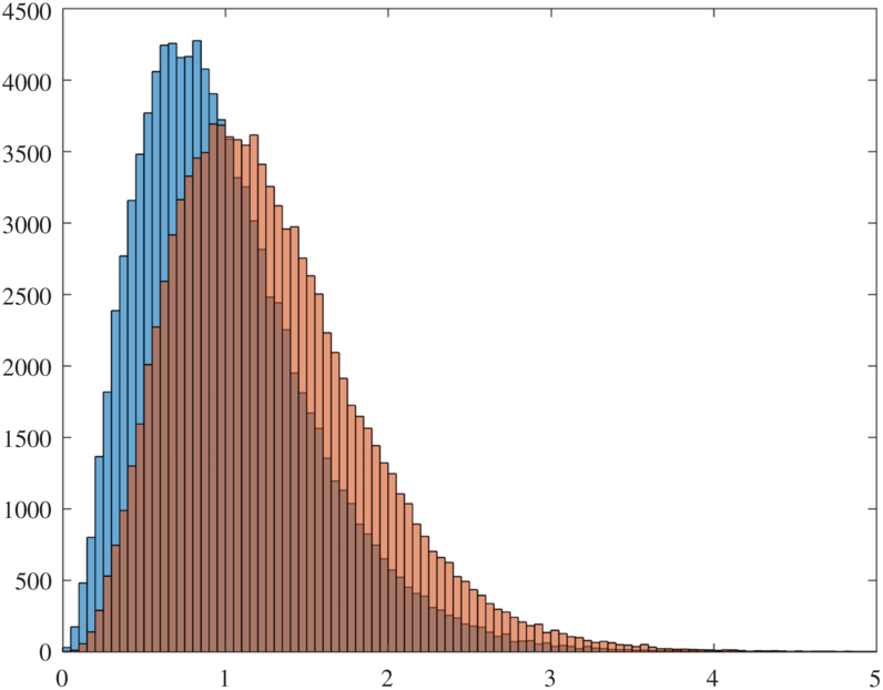
Since both the distribution of Z and that of Y are independent of f or x, we are able to obtain information about these distributions by numerically simulating $n\mu_{f}\left(L_{n}\left(x\right)\right)$ and $n\mu_{f}\left(A_{n}\left(x\right)\right)$ for large n with $f=2^{-d}\mathbb{I}_{\left(-1,1\right)^{d}}$ and $x=0$ . We generate the histogram estimate of the density for both limiting distributions in the case $d=2$ and place them together in Figure 2. It is clear from the comparison that, as stated by Theorem 3.2, the limiting distribution of $n\mu_{f}\left(L_{n}\left(x\right)\right)$ gives higher probabilities to larger values than that of $n\mu_{f}\left(A_{n}\left(x\right)\right)$ .

Figure 2:

Histogram of the density estimate of the limiting distribution of $n\mu_{f}\left(L_{n}\left(x\right)\right)$ (copper) and $n\mu_{f}\left(A_{n}\left(x\right)\right)$ (blue). One thousand samples of the Voronoi diagram arising from the point process $\left\{ X_{1},\cdots,X_{1000}\right\} $ that is composed of i.i.d. random variables with the uniform distribution on $\left[-1,1\right]^{2}$ were taken. $n\mu_{f}\left(L_{n}\left(0\right)\right)$ and $n\mu_{f}\left(A_{n}\left(0\right)\right)$ were calculated for each trial and the resulting data was grouped together into bins of width 0.05. The x-axis indicates the observed values for $n\mu_{f}\left(L_{n}\left(0\right)\right)$ and $n\mu_{f}\left(A_{n}\left(0\right)\right)$ while the y-axis shows the number of occurrences of values in each bin. The authors are grateful to Jean-Christophe Nave for performing the simulations of the two limiting distributions and generating the histogram figures.

Theorem 3.2. Let f be any probability density function on $\mathbb{R}^{d}$ , and let x be a Lebesgue point of f such that $f\left(x\right)>0$ . There exists a random variable Z, whose distribution is universal in f and x, such that $n\mu_{f}\left(L_{n}\left(x\right)\right)$ converges in distribution to Z as $n\rightarrow\infty$ . In addition, for every $k\geq1$ ,

\begin{align*}\mathbb{E}\left[Z^{k}\right]&=\lim\limits _{n\rightarrow\infty}\mathbb{E}\left[n^{k}\mu_{f}\left(L_{n}\left(x\right)\right)^{k}\right]=\lim\limits _{n\rightarrow\infty}\mathbb{E}\left[n^{k+1}\mu_{f}\left(A_{n}\left(x\right)\right)^{k+1}\right]\\[4pt] &=\mathbb{E}\left[Y^{k+1}\right]=\mathbb{E}\left[\frac{(k+1)!}{W_{k+1}^{k+1}}\right],\end{align*}

where Y and $\left\{ W_{k}\,{:}\,k\geq1\right\} $ are the same as in Theorem 3.1 of Devroye et al. [Reference Devroye, Györfi, Lugosi and Walk7].

Proof. Step 1. Existence of the limiting distribution of $n\mu_{f}\left(L_{n}\left(x\right)\right)$ . By Proposition 3.2 and Slutsky’s theorem, in order to get the limiting distribution of $n\mu_{f}\left(L_{n}\left(x\right)\right)$ , it is enough to study the limiting distribution of $nf\left(x\right)\lambda\left(L_{n}\left(x\right)\right)$ as $n\rightarrow\infty$ . We recall that, for every $\Lambda>0$ and $y\in\mathbb{R}^{d}$ , $P_{\Lambda}$ is a Poisson point process with density $\Lambda$ and $P_{\Lambda}^{L}\left(y\right)$ is the cell containing y in the Voronoi diagram generated by $P_{\Lambda}$ . Then, by Proposition 3.1 we have that

\begin{equation*}\lim_{n\rightarrow\infty}\sup_{z\in\mathbb{R}}\left|\mathbb{P}\bigg(nf\left(x\right)\lambda\left(L_{n}\left(x\right)\right)\leq z\bigg)-\mathbb{P}\bigg(nf\left(x\right)\lambda\left(P_{nf\left(x\right)}^{L}\left(x\right)\right)\leq z\bigg)\right|=0.\end{equation*}

Thus, we only need to examine the distribution of $nf\left(x\right)\lambda\big(P_{nf\left(x\right)}^{L}\left(x\right)\big)$ , which in fact is identical for all n, f, and x. In particular, we claim that for every $\Lambda,\Lambda^{\prime}>0$ and $x,y\in\mathbb{R}^{d}$ ,

(13) \begin{equation}\begin{split}\Lambda\lambda\left(P_{\Lambda}^{L}\left(x\right)\right)\stackrel{\text{ in dist. }}{=}\Lambda^{\prime}\lambda\left(P_{\Lambda^{\prime}}^{L}\left(y\right)\right)\end{split}\end{equation}

where ‘ $\overset{\text{in dist.}}{=}$ ’ refers to equality in distribution. The fact that the distribution of $\Lambda\lambda(P_{\Lambda}^{L}(x))$ is independent of x is immediate from the definition of $P_{\Lambda}$ . To further see that ( $13$ ) holds when $x=y=0$ , one simply notes that the map $T\,{:}\,y\in\mathbb{R}^{d}\mapsto T\left(y\right): \left(\Lambda/\Lambda^{\prime}\right)^{1/d}y$ satisfies that $T\left(P_{\Lambda}\right)\stackrel{\text{in dist.}}{=}P_{\Lambda'}$ and $\Lambda^{\prime}\lambda\left(T\left(P_{\Lambda}^{L}\left(0\right)\right)\right)=\Lambda\lambda\left(P_{\Lambda}^{L}\left(0\right)\right)$ . Therefore, we can conclude that $n\mu_{f}\left(L_{n}\left(x\right)\right)$ converges in distribution as $n\rightarrow\infty$ , and the limiting distribution is independent of f or x.

Step 2. Convergence of the moments of $n\mu_{f}\left(L_{n}\left(x\right)\right)$ . We have proven in the previous step that $n\mu_{f}\left(L_{n}\left(x\right)\right)$ converge in distribution to a random variable, say, Z, as $n\rightarrow\infty$ . In order to show that all the moments of $n\mu_{f}\left(L_{n}\left(x\right)\right)$ also converge to the corresponding moments of Z, it suffices to verify the boundedness of all the moments in n (see, e.g., Billingsley [3, Theorem 25.12]), i.e., to show that

\begin{equation*}\sup_{n\geq1}n^{k}\mathbb{E}\left[\left(\mu_{f}\left(L_{n}\left(x\right)\right)\right)^{k}\right]<\infty \quad \forall k\geq1.\end{equation*}

Let $k\geq1$ be fixed. Again, by the Lebesgue differentiation theorem, we may choose $\delta>0$ such that if $y\in B_{x,\delta}$ , then $\left|\frac{\mu_{f}\left(B_{x,||x-y||}\right)}{\lambda\left(B_{x,||x-y||}\right)}-f(x)\right|<\frac{1}{2}\,f(x)$ . Then, it follows that for all n sufficiently large,

\begin{equation*}\begin{split}n^{k}\mathbb{E}\left[\left(\mu_{f}\left(L_{n}\left(x\right)\right)\right)^{k}\right] & =n^{k}\int_{0}^{1}\mathbb{P}\left(\mu_{f}\left(L_{n}\left(x\right)\right)>y\right)ky^{k-1}dy\\ & \leq n^{k}\int_{0}^{1}\mathbb{P}\big(\mu_{f}\big(B_{x,D_{n}^{L}(x)}\big)>y\big)ky^{k-1}dy\\ & \leq n^{k}\int_{0}^{1}\mathbb{P}\left(\!\lambda\big(B_{x,D_{n}^{L}(x)}\big)>\frac{2y}{3f\left(x\right)},\ D_{n}^{L}(x)<\delta)\!\right)ky^{k-1}dy+\mathbb{P}\left(D_{n}^{L}(x)\geq\delta\right)n^{k}\\ & \leq n^{k}\int_{0}^{\delta}\mathbb{P}\left(\delta>D_{n}^{L}(x)>\left(\frac{2y}{3f\left(x\right)\lambda_{0}}\right)^{1/d}\right)ky^{k-1}dy+\mathbb{P}\left(D_{n}^{L}(x)\geq\delta\right)n^{k}\\ & \leq c_{1}n^{k}\int_{0}^{\delta}e^{-\frac{-2yc_{2}n}{3\lambda_{0}}}ky^{k-1}dy+c_{1}e^{-c_{2}n\delta^{d}f\left(x\right)}n^{k},\end{split}\end{equation*}

where the last inequality follows from Theorem 3.1. By integrating the first term in the last line by parts $k-1$ times, one immediately finds that this quantity is uniformly bounded in n.

Step 3. Boundedness of the moments inn andx. With the results of Step 1 and Step 2 in hand we see that without loss of generality we can choose $f: \lambda_{0}^{-1}\mathbb{I}_{B_{0,1}}$ , where we recall that $\lambda_{0}: \lambda(B_{0,1})$ . Then $\mu_{f}=\lambda_{0}^{-1}\lambda|_{B_{0,1}}$ , and every $x\in B_{0,1}$ is a Lebesgue point of f, with $f\left(x\right)>0$ . For this specific choice of f, our goal is to establish the boundedness of all the moments of $n\mu_{f}\left(L_{n}\left(x\right)\right)$ in both n and admissible x, i.e., to show that

(14) \begin{equation}\sup_{x\in B_{0,1}}\sup_{n}n^{k}\mathbb{E}\left[\mu_{f}\left(L_{n}\left(x\right)\right)^{k}\right]<\infty \quad \forall k\geq1.\end{equation}

Let $k\geq1$ be fixed, and let $X_{n+1},\cdots,X_{n+k}$ be i.i.d. copies of $X_{1}$ , independent of $\left\{ X_{1},\cdots,X_{n}\right\} $ . Similarly as in Proposition 2.1, we have that $n^{k}\mathbb{E}\left[\mu_{f}\left(L_{n}\left(x\right)\right)^{k}\right]$ is equal to

\begin{equation*}\begin{split} & n^{k}\mathbb{P}\left(X_{n+1},\cdots,X_{n+k}\in L_{n}\left(x\right)\right)\\[3pt] & = n^{k}\sum_{i=1}^{n}\mathbb{P}\left(x\in A_{n}^{*}\left(X_{i}\right)\!,\,X_{n+1},\cdots,X_{n+k}\in L_{n}\left(x\right)\right)\\[3pt] & = n^{k+1}\mathbb{P}\left(x\in A_{n}^{*}\left(X_{1}\right)\!,\,X_{n+1},\cdots,X_{n+k}\in L_{n}\left(x\right)\right)\\[3pt] & = n^{k+1}\mathbb{P}\left(x\in A_{n}^{*}\left(X_{1}\right)\!,\,X_{n+1},\cdots,X_{n+k}\in A_{n}^{*}\left(X_{1}\right)\right)\\[3pt] & = n^{k+1}\mathbb{P}\left(X_{i}\notin\bigcup_{j=1}^{k}B_{X_{n+j},\left\Vert X_{n+j}-X_{1}\right\Vert }\cup B_{x,\left\Vert x-X_{1}\right\Vert },\,i\in\left\{ 2,\cdots,n\right\} \right)\\[3pt] & = n^{k+1}\mathbb{E}\left[\left(1-\lambda_{0}^{-1}\lambda\left(B_{0,1}\cap\bigcup_{j=1}^{k}B_{X_{n+j},\left\Vert X_{n+j}-X_{1}\right\Vert }\cup B_{x,\left\Vert x-X_{1}\right\Vert }\right)\right)^{n-1}\right].\end{split}\end{equation*}

By the same arguments as those employed in the derivation of (8), in order to show that the right-hand side above is bounded in n and x, it is sufficient to verify that there exist $M,\eta>0$ such that for every $x\in B_{0,1}$ and $z\in\left(0,\eta\right)$ ,

\begin{equation*}z^{-k-1}\mathbb{P}\left(\lambda\left(B_{0,1}\cap\bigcup_{j=1}^{k}B_{X_{n+j},\left\Vert X_{n+j}-X_{1}\right\Vert }\cup B_{x,\left\Vert x-X_{1}\right\Vert }\right)\leq\lambda_{0}z\right)<M.\end{equation*}

The quantity above can be estimated as follows:

\begin{equation*}\begin{split} & z^{-k-1}\mathbb{P}\left(\lambda\left(B_{0,1}\cap\bigcup_{j=1}^{k}B_{X_{n+j},\left\Vert X_{n+j}-X_{1}\right\Vert }\cup B_{x,\left\Vert x-X_{1}\right\Vert }\right)\leq\lambda_{0}z\right)\\[3pt] & \quad\leq z^{-k-1}\mathbb{P}\left(\lambda\left(B_{0,1}\cap B_{x,\left\Vert x-X_{1}\right\Vert }\right)\leq\lambda_{0}z,\,\lambda\left(B_{0,1}\cap B_{X_{n+j},\left\Vert X_{n+j}-X_{1}\right\Vert }\right)\leq\lambda_{0}z,\,j\in\left\{ 1,\cdots,k\right\} \right)\\[3pt] & \quad \leq \lambda_{0}^{-1}z^{-k-1}\int_{\left\{ y\in B_{0,1}:\lambda\left(B_{0,1}\cap B_{x,||x-y||}\right)\leq\lambda_{0}z\right\} }\left(\lambda_{0}^{-1}\lambda\left(D_{y}\right)\right)^{k}dy\\[3pt] &\quad = \lambda_{0}^{-k-1}z^{-k-1}\int_{B_{0,1}}\mathbb{I}_{D_{x}}\left(y\right)\left(\lambda\left(D_{y}\right)\right)^{k}dy,\end{split}\end{equation*}

where for every $y\in B_{0,1}$ , $D_{y}$ is the subset of $B_{0,1}$ given by

\begin{equation*}D_{y}: \left\{ w\in B_{0,1}\,{:}\,\lambda\left(B_{0,1}\cap B_{w,\left\Vert w-y\right\Vert }\right)\leq\lambda_{0}z\right\} .\end{equation*}

Obviously, when $y\in B_{0,1-2z^{1/d}}$ , $D_{y}$ coincides with $B_{y,z^{1/d}}$ . For general $y\in B_{0,1}$ , we have that $D_{y}\subseteq B_{y,3z^{1/d}}$ . To see this, we observe that if $C_{w}$ , $w\in B_{0,1}$ , is the cone originated from w, centered around the line connecting w and 0 with an angle of $\frac{\pi}{4}$ , then $C_{w}\cap B_{w,3z^{1/d}}\subseteq B_{0,1}$ when z is sufficiently small. Thus, if $\left\Vert w-y\right\Vert >3z^{1/d}$ , then

\begin{equation*}\lambda\left(B_{0,1}\cap B_{w,\left\Vert w-y\right\Vert }\right)\geq\lambda\left(B_{0,1}\cap B_{w,3z^{1/d}}\right)\geq\lambda\left(C_{w}\cap B_{w,3z^{1/d}}\right)=\frac{3^{d}\lambda_{0}z}{2^{d}}>\lambda_{0}z,\end{equation*}

which means that $w\notin D_{y}$ . Therefore, we have that for every $y\in B_{0,1}$ , $\lambda\left(D_{y}\right)\leq\lambda\left(B_{y,3z^{1/d}}\right)=\lambda_{0}3^{d}z$ . It follows from here that for all $z>0$ sufficiently small,

\begin{equation*}\begin{split} & z^{-k-1}\mathbb{P}\left(\lambda\left(B_{0,1}\cap\bigcup_{j=1}^{k}B_{X_{n+j},\left\Vert X_{n+j}-X_{1}\right\Vert }\cup B_{x,\left\Vert x-X_{1}\right\Vert }\right)\leq\lambda_{0}z\right)\\[3pt] & \quad \leq \lambda_{0}^{-k-1}z^{-k-1}\int_{B_{0,1}}\mathbb{I}_{D_{x}}\left(y\right)\left(\lambda\left(D_{y}\right)\right)^{k}dy\leq3^{\left(k+1\right)d},\end{split}\end{equation*}

which is exactly what we want, and hence (14) is proven.

We can treat the kth moment of $n\mu_{f}\left(A_{n}\left(x\right)\right)$ in exactly the same way. To be specific,

\begin{equation*}\begin{split}n^{k}\mathbb{E}\left[\left(\mu_{f}\left(A_{n}\left(x\right)\right)\right)^{k}\right] & =n^{k}\mathbb{P}\left(X_{n+1},\dots,X_{n+k}\in A_{n}\left(x\right)\right)\\ & =n^{k}\mathbb{E}\left[\left(1-\lambda_{0}^{-1}\lambda\left(\bigcup_{j=1}^{k}B_{X_{n+j},\left\Vert X_{n+j}-x\right\Vert }\cap B_{0,1}\right)\right)^{n}\right],\end{split}\end{equation*}

and for all $z>0$ sufficiently small,

\begin{equation*}\begin{split}z^{-k}\mathbb{P}\left(\lambda\left(\bigcup_{j=1}^{k}B_{X_{n+j},\left\Vert X_{n+j}-x\right\Vert }\right)\leq\lambda_{0}z\right) & \le z^{-k}\mathbb{P}\left(\bigcap_{j=i}^{k}\left\{ \lambda\left(B_{X_{n+j},\left\Vert X_{n+j}-x\right\Vert }\cap B_{0,1}\right)\leq\lambda_{0}z\right\} \right)\\ & =z^{-k}\left(\lambda_{0}^{-1}\lambda\left(D_{x}\right)\right)^{k}\leq3^{dk}.\end{split}\end{equation*}

Therefore, following a similar argument as above, we have that

(15) \begin{equation}\sup_{x\in B_{0,1}}\sup_{n}n^{k}\mathbb{E}\big[\mu_{f}\left(A_{n}\left(x\right)\right)^{k}\big]<\infty.\end{equation}

Step 4. Connection between the moments of Z and the moments of Y. Finally we are ready to establish the relation between the limiting distribution of $n\mu_{f}\left(L_{n}\left(x\right)\right)$ and that of $n\mu_{f}\left(A_{n}\left(x\right)\right)$ , i.e., the relation between the distribution of Z and that of Y. Again, let $\left\{ X_{n+1},\cdots,X_{n+k+1},\cdots\right\} $ be a family of i.i.d. copies of $X_{1}$ , independent of $\left\{ X_{1},\cdots,X_{n}\right\} $ , and let $f=\lambda_{0}^{-1}\mathbb{I}_{B_{0,1}}$ for now. By (14) and the dominated convergence theorem, we have that for every $k\geq1$ ,

\begin{equation*}\lim_{n\rightarrow\infty}n^{k}\mathbb{E}\left[\left(\mu_{f}\left(L_{n}\left(X_{n+1}\right)\right)\right)^{k}\right]=\lambda_{0}^{-1}\int_{B_{0,1}}\lim_{n\rightarrow\infty}n^{k}\mathbb{E}\left[\left(\mu_{f}\left(L_{n}\left(x\right)\right)\right)^{k}\right]dx=\mathbb{E}\big[Z^{k}\big].\end{equation*}

Meanwhile,

\begin{align*}\lim_{n\rightarrow\infty}n^{k}\mathbb{E}\left[\left(\mu_{f}\left(L_{n}\left(X_{n+1}\right)\right)\right)^{k}\right] & =\lim_{n\rightarrow\infty}n^{k}\mathbb{P}\left(X_{n+2},\cdots,X_{n+k+1}\in L_{n}\left(X_{n+1}\right)\right)\\[4pt] & =\lim_{n\rightarrow\infty}n^{k}\sum_{j=1}^{n}\mathbb{P}\left(X_{n+2},\cdots,X_{n+k+1}\in A_{n}^{*}\left(X_{j}\right)\!,X_{n+1}\in A_{n}^{*}\left(X_{j}\right)\right)\\[4pt] & =\lim_{n\rightarrow\infty}n^{k+1}\mathbb{P}\left(X_{n+1},X_{n+2},\cdots,X_{n+k+1}\in A_{n}^{*}\left(X_{1}\right)\right)\\ & =\lim_{n\rightarrow\infty}n^{k+1}\mathbb{E}\left[\left(\mu_{f}\left(A_{n}^{*}\left(X_{1}\right)\right)\right)^{k+1}\right]\\[4pt] & =\lim_{n\rightarrow\infty}\lambda_{0}^{-1}\int_{B_{0,1}}n^{k+1}\mathbb{E}\Big[\left(\mu_{f}\left(A_{n}\left(x\right)\right)\right)^{k+1}\Big]dx\\[4pt] & =\lambda_{0}^{-1}\int_{B_{0,1}}\lim_{n\rightarrow\infty}n^{k+1}\mathbb{E}\Big[\left(\mu_{f}\left(A_{n}\left(x\right)\right)\right)^{k+1}\Big]dx\\[4pt] & =\mathbb{E}\big[Y^{k+1}\big],\end{align*}

where the second last equality is due to (15) and, again, the dominated convergence theorem, and the last equality is the result from Devroye et al. [Reference Devroye, Györfi, Lugosi and Walk7]. Thus we have proven that $\mathbb{E}[Z^{k}]=\mathbb{E}[Y^{k+1}]$ for every $k\geq1$ , or equivalently, for any f a probability density function on $\mathbb{R}^{d}$ and x a Lebesgue point of f such that $f\left(x\right)>0$ ,

\begin{align*}\lim\limits _{n\rightarrow\infty}\mathbb{E}\big[n^{k}\mu_{f}\left(L_{n}\left(x\right)\right)^{k}\big]=\lim\limits _{n\rightarrow\infty}\mathbb{E}\big[n^{k+1}\mu_{f}\left(A_{n}\left(x\right)\right)^{k+1}\big] \quad \forall k\geq1.\end{align*}

The proof of Theorem 3.2 is completed.□

A Appendix

Lemma A.1. Let $\alpha>0$ and $x\in\mathbb{R}^{d}$ , and let $C\subseteq\mathbb{R}^{d}$ be any cone of angle $\pi/12$ and with origin at x (C does not contain x); i.e.,

\begin{equation*}C: \left\{ y\in\mathbb{R}^{d}\backslash\left\{ x\right\} :\frac{\left(v,y-x\right)_{\mathbb{R}^{d}}}{\left\Vert y-x\right\Vert }\geq\cos\left(\frac{\pi}{24}\right)\right\} \quad for\ some\ v\in\mathbb{R}^{d}\ with\ \left\Vert v\right\Vert =1.\end{equation*}

Set

\begin{equation*}R_{1}: \frac{1}{64}\alpha,\ R_{2}: \frac{1+31\cos\left(\frac{\pi}{6}\right)}{64\cos\left(\frac{\pi}{12}\right)}\alpha,\ and\ R_{3}: \frac{30}{64}\alpha.\end{equation*}

For any $p,y,z\in C$ , if

\begin{equation*}0<\left\Vert y-x\right\Vert <R_{1},\ R_{2}\leq\left\Vert p-x\right\Vert <R_{3},\ and\ \left\Vert x-z\right\Vert \geq\frac{\alpha}{2},\end{equation*}

then we have that

\begin{equation*}\left\Vert z-p\right\Vert <\left\Vert z-y\right\Vert .\end{equation*}

Proof. We claim that it is enough to prove this lemma in the case $d=2$ . First, note that by translation we may assume that $x=0$ . Then, let $y^{\prime}$ be the point on the line segment connecting 0 and z such that $\left\Vert y^{\prime}\right\Vert =\left\Vert y\right\Vert $ . It should be clear that $\left\Vert y^{\prime}-z\right\Vert \leq\left\Vert y-z\right\Vert $ . Hence, without loss of generality we may assume that $y=y^{\prime}$ . Use the Gram–Schmidt process to complete $\left\{ p,y\right\} $ to an orthonormal basis of $\mathbb{R}^{d}$ , and consider the problem in this basis. Since the Euclidean inner product is invariant under orthogonal transformations, both the Euclidean norm and the cone, C, will be preserved by this transformation. Additionally, by the use of Gram–Schmidt, we will have that in the new basis, $p=\left(p_{1},0,\cdots,0\right)$ , $y=\left(y_{1},y_{2},0,\cdots,0\right)$ , and $z=\left(z_{1},z_{2},0,\cdots,0\right)$ for some $p_{1},y_{1},y_{2},z_{1},z_{2}\in\mathbb{R}$ . Thus, we see that we may assume that $d=2$ .

Figure A1 outlines the current setting. First we remark that

\begin{equation*}\begin{split}\left\Vert y-p\right\Vert ^{2} & =\left\Vert x-y\right\Vert ^{2}+\left\Vert x-p\right\Vert ^{2}-2\left\Vert x-y\right\Vert \left\Vert x-p\right\Vert \cos\xi\\ & \leq\left\Vert x-y\right\Vert ^{2}+\left\Vert x-p\right\Vert ^{2}-2\left\Vert x-y\right\Vert \left\Vert x-p\right\Vert \cos\left(\frac{\pi}{12}\right)\!.\end{split}\end{equation*}

Moreover,

\begin{equation*}\begin{split}\left\Vert x-p\right\Vert ^{2} & =\left\Vert x-y\right\Vert ^{2}+\left\Vert y-p\right\Vert ^{2}-2\left\Vert x-y\right\Vert \left\Vert y-p\right\Vert \cos\phi\\ & \leq2\left\Vert x-y\right\Vert ^{2}+\left\Vert x-p\right\Vert ^{2}-2\left\Vert x-y\right\Vert \left\Vert x-p\right\Vert \cos\left(\frac{\pi}{12}\right)-2\left\Vert x-y\right\Vert \left\Vert y-p\right\Vert \cos\left(\phi\right)\!.\end{split}\end{equation*}

Rewriting the inequality above gives

\begin{equation*}\cos\phi\leq\frac{\left\Vert x-y\right\Vert -\left\Vert x-p\right\Vert \cos\left(\pi/12\right)}{\left\Vert y-p\right\Vert }\leq\frac{R_{1}-R_{2}\cos\left(\pi/12\right)}{R_{3}+R_{1}}.\end{equation*}

Plugging in the values of $R_{1}$ , $R_{2}$ , and $R_{3}$ , we get that $\phi\geq5\pi/6$ and $\beta=\pi-\phi\leq\pi/6$ .

Figure A1:

Diagram of the setting under study in Lemma A.1.

Now assume the conclusion fails, i.e., $\left\Vert z-y\right\Vert \leq\left\Vert z-p\right\Vert $ . Then

\begin{equation*}\begin{split}\left\Vert z-p\right\Vert ^{2} & =\left\Vert z-y\right\Vert ^{2}+\left\Vert y-p\right\Vert ^{2}-2\left\Vert z-y\right\Vert \left\Vert y-p\right\Vert \cos\beta\\ & \leq\left\Vert z-y\right\Vert ^{2}+\left\Vert y-p\right\Vert ^{2}-2\left\Vert z-y\right\Vert \left\Vert y-p\right\Vert \cos\left(\frac{\pi}{6}\right)\\ & \leq\left\Vert z-p\right\Vert ^{2}+\left\Vert y-p\right\Vert ^{2}-2\left\Vert z-y\right\Vert \left\Vert y-p\right\Vert \cos\left(\frac{\pi}{6}\right)\!,\end{split}\end{equation*}

and so

\begin{equation*}\left\Vert z-y\right\Vert \leq\frac{\left\Vert y-p\right\Vert }{2\cos\left(\pi/6\right)}\leq\frac{R_{1}+R_{3}}{2\cos\left(\pi/6\right)},\end{equation*}

which implies that

\begin{equation*}\left\Vert z-x\right\Vert \leq\left\Vert z-y\right\Vert +\left\Vert y-x\right\Vert \leq\frac{R_{1}+R_{3}}{2\cos\left(\pi/6\right)}+R_{1}<\frac{\alpha}{2}.\end{equation*}

This contradicts the assumption that $\left\Vert z-x\right\Vert \geq\alpha/2$ and thus concludes the proof.□

Lemma A.2. Let g be a probability density function on $\mathbb{R}^{d}$ , and let x be a Lebesgue point of g such that $g\left(x\right)>0$ . For any $c,r>0$ define the set

\begin{equation*}\mathscr{Q}_{c,r}: \{Q\subseteq\mathbb{R}^{d}\,:\,\frac{\lambda(Q^{*})}{\lambda(Q)}\leq c\ and\ \lambda(Q)\leq r\},\end{equation*}

where $Q^{*}$ denotes the smallest ball centered at x that contains Q. Then

\begin{equation*}\lim_{r\rightarrow0}\sup_{Q\in\mathscr{Q}_{c,r}}\int_{Q}\left|\frac{g\left(u\right)}{\mu_{g}\left(Q\right)}-\frac{1}{\lambda\left(Q\right)}\right|du=0.\end{equation*}

Proof. By the generalized Lebesgue differentiation theorem (see, e.g., Theorem 20.19 of Devroye and Biau [Reference Biau and Devroye2] and Theorem 5.3 of Devroye and Lugosi [Reference Devroye and Lugosi9]) we have that for every $\epsilon\in(0,1)$ , there exists $\delta>0$ such that for every $Q\in\mathscr{Q}_{c,\delta}$ ,

\begin{equation*}\frac{1}{\lambda\left(Q^{*}\right)}\int_{Q^{*}}\left|g\left(u\right)-g\left(x\right)\right|du\leq\frac{\epsilon g\left(x\right)}{3c},\end{equation*}

\begin{equation*}\left|\frac{\mu_{g}\left(Q\right)}{\lambda\left(Q\right)}-g\left(x\right)\right|\leq\frac{\epsilon g\left(x\right)}{3},\end{equation*}

and

\begin{equation*}\left|\frac{\lambda\left(Q\right)}{\mu_{g}\left(Q\right)}-\frac{1}{g\left(x\right)}\right|\leq\frac{\epsilon}{3g\left(x\right)}.\end{equation*}

Then, for any $Q\in\mathscr{Q}_{c,\delta}$ , we have that

\begin{equation*}\begin{split}\int_{Q}\left|\frac{g\left(u\right)}{\mu_{g}\left(Q\right)}-\frac{1}{\lambda\left(Q\right)}\right|du & =\frac{1}{\mu_{g}\left(Q\right)}\int_{Q}\left|g\left(u\right)-\frac{\mu_{g}\left(Q\right)}{\lambda\left(Q\right)}\right|du\\[5pt] & =\frac{\lambda\left(Q\right)}{\mu_{g}\left(Q\right)}\frac{1}{\lambda\left(Q\right)}\int_{Q}\left|g\left(u\right)-g\left(x\right)\right|du+\frac{\lambda\left(Q\right)}{\mu_{g}\left(Q\right)}\left|g\left(x\right)-\frac{\mu_{g}\left(Q\right)}{\lambda\left(Q\right)}\right|\\[5pt] & \leq\frac{\lambda\left(Q\right)}{\mu_{g}\left(Q\right)}\frac{c}{\lambda(Q^{*})}\int_{Q^{*}}\left|g\left(u\right)-g\left(x\right)\right|du+\frac{\lambda\left(Q\right)}{\mu_{g}\left(Q\right)}\left|g\left(x\right)-\frac{\mu_{g}\left(Q\right)}{\lambda\left(Q\right)}\right|\\[5pt] & \leq\left(\frac{1}{g\left(x\right)}+\frac{\epsilon}{3g\left(x\right)}\right)\frac{\epsilon g\left(x\right)}{3}+\left(\frac{1}{g\left(x\right)}+\frac{\epsilon}{3g\left(x\right)}\right)\frac{\epsilon g\left(x\right)}{3}\leq\epsilon,\end{split}\end{equation*}

from which the desired result immediately follows.□