1. Introduction
Buoyancy-driven flow is a fundamental phenomenon observed in various natural flows, including atmospheric convection (Hartmann, Moy & Fu Reference Hartmann, Moy and Fu2001), ocean convection (Van Doorn et al. Reference Van Doorn, Dhruva, Sreenivasan and Cassella2000) and geophysical convection (Glatzmaier et al. Reference Glatzmaier, Coe, Hongre and Roberts1999). Turbulent Rayleigh–Bénard convection (RBC) is a widely studied system for investigating buoyancy-driven flow (Ahlers, Grossmann & Lohse Reference Ahlers, Grossmann and Lohse2009; Lohse & Xia Reference Lohse and Xia2010; Chilla & Schumacher Reference Chilla and Schumacher2012; Xia Reference Xia2013; Xia et al. Reference Xia, Huang, Xie and Zhang2023), where a fluid layer is heated from the bottom and cooled from the top. Such RBC is characterised by three control parameters: the Rayleigh number (
 $Ra$
), the Prandtl number (
 $Pr$
), and the aspect ratio (
 $\Gamma$
). The Rayleigh number quantifies the strength of the buoyancy force relative to thermal and viscous dissipative effects, and is defined as
 $Ra = \alpha g\, \Delta T\,H^3/(\nu \kappa )$
. Here,
 $\alpha$
,
 $\nu$
and
 $\kappa$
represent the thermal expansion coefficient, kinematic viscosity and thermal diffusivity of the fluid, respectively. The parameter
 $g$
is the gravitational acceleration,
 $\Delta T$
is the temperature difference across the bottom and top plates, and
 $H$
is the height of the convection cell. The Prandtl number (
 $Pr = \nu /\kappa$
) is the ratio of viscosity to thermal diffusivity. Cylindrical convection cells are frequently employed due to their azimuthal symmetry. The aspect ratio of the cylindrical cell is defined as
 $\Gamma = D/H$
, where
 $D$
is the diameter of the cylindrical cell.
Recently, extensive studies have been focused on the convection in very slender (very small
 $\Gamma$
) convection cells due to their advantage in achieving very high
 $Ra$
with less additional experimental or computational effort (Cheng et al. Reference Cheng, Madonia, Guzmán and Kunnen2020; Iyer et al. Reference Iyer, Scheel, Schumacher and Sreenivasan2020), as
 $Ra$
increases with the third power of
 $H$
. Very slender cells introduce severe spatial confinement to the flow (Nikolaenko et al. Reference Nikolaenko, Brown, Funfschilling and Ahlers2005; Hartmann et al. Reference Hartmann, Chong, Stevens, Verzicco and Lohse2021; Zhang & Xia Reference Zhang and Xia2023; Kashanj & Nobes Reference Kashanj and Nobes2023; Noto, Letelier & Ulloa Reference Noto, Letelier and Ulloa2024; Ren et al. Reference Ren, Tao, Xia and Xie2024), thus it is crucial to understand how lateral confinement affects the topology and dynamics of the flow. However, studies on the flow topology in the very slender cells are very limited. And the few existing studies are limited to numerical simulation. In
 $\Gamma =1/5$
cells, Zwirner, Tilgner & Shishkina (Reference Zwirner, Tilgner and Shishkina2020) observed in their direct numerical simulations (DNS) that for
 $Ra=5 \times 10^{6}$
and
 $Pr = 0.1$
, the large-scale circulation (LSC) comprises varying numbers of convective rolls stacked on top of each other. The number of the stacked rolls varies from 1 to 4, with the vertically stacked double-roll being the most prevalent. In addition, the twisting and breaking of the single-roll into multiple rolls were well explained by using the elliptical instability. In the slender cell such as
 $\Gamma =1/5$
, one may expect that the flow would be in the form of vertically stacked five aspect ratio unity rolls, however Zwirner et al. (Reference Zwirner, Tilgner and Shishkina2020) did not observe the existence of five-roll structure during their simulations. Iyer et al. (Reference Iyer, Scheel, Schumacher and Sreenivasan2020) conducted a DNS study in a cylindrical cell with
 $\Gamma = 1/10$
, and found a persistent helical large-scale flow structure across the entire range
 $10^{8} \leqslant Ra \leqslant 10^{15}$
, with
 $Pr$
held fixed at unity. Although they mentioned the occasional collapses of this helical structure, the feature of the helical flow remains robust. A numerical study by Hartmann et al. (Reference Hartmann, Chong, Stevens, Verzicco and Lohse2021) found that for the
 $\Gamma = 1/7$
and
 $1/10$
cases at
 $Ra = 2 \times 10^8$
,
 $Pr = 4.38$
, thermal plumes descend and ascend along the sidewalls near the top and bottom boundaries. These ascending and descending plumes merge at certain heights, forming a single-roll flow structure before impinging on the opposite boundaries at the centre of the top/bottom plate. Additionally, they noted the existence of a lower sublayer (
 $0 \leqslant z/H \leqslant 0.2$
) for the
 $\Gamma = 1/10$
case that is absent near the top boundaries. The above-mentioned three representative studies report three very different flow topologies in the very slender cell, namely, the multiple-roll structure, the helical structure and the single-roll-like structure. It is important to note that the above-mentioned three major numerical studies were not performed under identical parameter ranges, and the initial conditions may also vary, which may account for the observed differences in flow topologies. Despite these variations, the three major numerical studies highlight three manifestations of the underlying flow dynamics within the very slender cylindrical cell. However, direct experimental measurements of the three-dimensional flow structure in such cells are currently lacking. Experimental investigations can provide valuable insights into the flow topology and dynamics in the very slender convection cells, serving as a crucial complement to these numerical studies. To our knowledge, the only experimental study regarding the flow structure conducted in similar
 $\Gamma$
is by Skuntz et al. (Reference Skuntz, Pelkie, Codd, Anderson and Seymour2020), who conducted velocity measurements using magnetic resonance velocimetry in a cylindrical cell with
 $\Gamma =0.12$
. However, it is important to note that magnetic resonance velocimetry provides only time-averaged fields, highlighting the continued urgency for direct and full-field three-dimensional velocity measurements in very small
 $\Gamma$
cells.
Besides the flow structures in the range of fully turbulent flow regimes reviewed above, early linear stability analyses and experiments had suggested that the critical
 $Ra$
for the onset of convection increases as
 $\Gamma$
decreases (Charlson & Sani Reference Charlson and Sani1971; Müller et al. Reference Müller, Neumann and Weber1984; Guthmann, Perrin & Thomé Reference Guthmann, Perrin and Thomé1989). Recently, Shishkina (Reference Shishkina2021) and Ahlers et al. (Reference Ahlers2022) predicted the influence of
 $\Gamma$
on both the onset
 $Ra$
and the critical
 $Ra$
for the ultimate regime based on theoretical and experimental data. Furthermore, Zhang & Xia (Reference Zhang and Xia2023) observed different flow patterns in the slender rectangular cells under different parameter ranges, with the onset
 $Ra$
scaling with
 $\Gamma ^{-4}$
. Additionally, several previous experiments based on temperature measurements have also reported results in slender cells with
 $\Gamma \leqslant 1$
. Cheng et al. (Reference Cheng, Madonia, Guzmán and Kunnen2020) utilised a very tall (height
 $4\ \text {m}$
) cylindrical cell with
 $\Gamma =0.097$
, allowing them to explore
 $Ra$
up to
 $10^{13}$
with water, although the scalings between Nusselt number
 $Nu$
and
 $Ra$
are found to remain consistent with previous results at moderate
 $Ra$
. Ren et al. (Reference Ren, Tao, Xia and Xie2024) measured heat transfer in liquid metal across multiple regimes from the onset of convection, noting that the transition to fully turbulent flow occurs at much smaller
 $Ra$
in smaller
 $\Gamma$
cells. However, it should be noted that multi-probe temperature measurements can provide only limited information about large-scale structures in small
 $\Gamma$
cells, especially where a predominant LSC may not exist.
The present study aims to bridge the knowledge gap regarding the flow structure inside a very slender RBC cell with
 $\Gamma =1/10$
by using tomographic particle image velocimetry (Tomo PIV). The Tomo PIV technique enables us to capture the three-dimensional, three-component velocity field with the measurement volume of the whole cell. It is worth noting that three-dimensional velocity measurements in turbulent RBC have been explored in only a few experimental studies. To date, the only study employing Tomo PIV in this context is that of Schiepel, Bosbach & Wagner (Reference Schiepel, Bosbach and Wagner2013), who investigated the three-dimensional characteristics of the LSC in a cubic cell. Apart from Tomo PIV, a limited number of studies (Ni, Huang & Xia Reference Ni, Huang and Xia2012; Godbersen et al. Reference Godbersen, Bosbach, Schanz and Schröder2021; Paolillo et al. Reference Paolillo, Greco, Astarita and Cardone2021; Weiss et al. Reference Weiss, Schanz, Erdogdu, Schröder and Bosbach2023) have utilised particle tracking velocimetry to obtain three-dimensional flow field information in turbulent RBC. Despite these efforts, the flow structure, especially three-dimensional flow structure, in the very slender RBC cells remains unexplored. By using Tomo PIV, our measurements provide insights into the instantaneous as well as spatio-temporal evolution of the flow field for the first time in such a very slender RBC cell. We further analyse and interpret the flow structure using mode decomposition analysis. The rest of the paper is organised as follows. In § 2, we describe the experiment set-up. In § 3, we present the experimental results and discussion. Finally, the conclusion of the study is drawn in § 4.
2. Experimental set-up
The convection cell used in the current study is shown in figure 1. It has height
 $H=19\ \text {cm}$
and a diameter
 $D=1.9\ \text {cm}$
, resulting in a fixed aspect ratio
 $\Gamma = D/H = 0.1$
. The convection cell consists of a bottom heating plate, a top cooling plate and the cylindrical Plexiglas sidewall. The bottom plate, made of oxygen-free copper of thickness
 $3\ \text {cm}$
and plated with a thin layer of nickel, ensures uniform temperature at the bottom boundary. The temperature of the bottom plate is regulated by circulating temperature-controlled heating water. For flow visualisation purposes, the top plate is a
 $5\ \text {mm}$
thick sapphire disc, providing good thermal conductivity and optical transparency. Above the sapphire plate is a Plexiglas water chamber filled with circulating water, connected to a water cooling device for temperature control. The temperature stability of the cooling and heating water is better than
 $0.01\ \text {K}$
(PolyScience). The sidewall, also made of Plexiglas, of length
 $192\ \text {mm}$
, has thermal conductivity
 $0.192\ \text {W}\ \text{m}^{-1}\ \text{K}^{-1}$
, providing nearly thermal insulation conditions. The temperature of the bottom plate is measured by four thermistors (Omega, 44031) inserted into the copper plate. These thermistors are positioned
 $2\ \text {mm}$
below the water–plate interface and at half of the radius from four different directions spaced by
 $90^\circ$
. Similarly, the temperature of the top plate is measured by two thermistors in contact with the side of the sapphire disc from two opposite directions. The accuracy of these thermistors is calibrated to better than
 $0.01\,^\circ {\rm C}$
. To measure the temperatures, a digital multimeter (Keysight, 34972A) was employed to measure the resistances of the six thermistors, at sampling rate
 $1\ \rm Hz$
. These resistances were then converted to temperatures using parameters obtained from a separate calibration process.
(a) Schematic diagram of the vertical cross-section of the convection cell. (b) Schematic diagram of the convection cell and the Tomo PIV system (only the four cameras and the laser beam are shown).

To facilitate Tomo PIV measurements, a Plexiglas tank with three flat surfaces is glued outside the cylindrical Plexiglas sidewall to reduce the distortion effect on the PIV images caused by the curvature of the sidewall, and the tank is filled with deionised water to match the refractive index. This tank has height approximately equal to that of the cell. To maximise the measurement volume of the Tomo PIV, we have machined a step on the top of the bottom plate with height
 $2\ \text {mm}$
and diameter
 $1.9\,\rm cm$
, which is fitted into the sidewall, as depicted in figure 1(a). Consequently, the height of the total measurement volume can be as large as
 $184\ \text {mm}$
.
The well-known Tomo PIV methods follow a common procedure as described in more detail in Scarano (Reference Scarano2012). In our experiments, four CCD cameras (Imperx Bobcat B3440) with 14-bit dynamic range and spatial resolution
 $3388 \times 2712$
pixels are used to capture the measurement volume under different angles of view. These cameras are arranged in the linear configuration with angle
 $30^\circ$
between each two cameras. The outer two cameras are equipped with
 $60\ \text {mm}$
focal length lenses, while the inner two cameras use
 $50\ \text {mm}$
focal length lenses. To save storage space, only the centre frame of the cameras with dimensions
 $3388 \times 500$
pixels is used. The fluid is seeded with tracer particles, which are made of polystyrene with diameter
 $d_p=20\,\unicode{x03BC} \rm m$
and density
 $\rho_p=1.02\,\rm g\,cm^{3}$
. The settling velocity
 $v_s$
due to the density mismatch between the fluid and the tracer particles is calculated by
 $v_s=(\rho _p-\rho )gd_{p}^{2}/18 \unicode{x03BC}$
, which is approximately
 $6.252 \times 10^{-9} \rm m\,s^-{^1}$
; here,
 $\unicode{x03BC}$
and
 $\rho$
are the dynamic viscosity and density of the fluid, respectively. These particles are illuminated by a pulsed volume laser beam and imaged by the cameras. The light source used in current experiments is a dual Nd:YAG laser (Beamtech Vlite-200) with power output
 $200\,\text{mJ}$
per pulse. The laser beam is expanded from a point source to a volume light beam using a combination of beam expanders, and then reflected by a mirror to illuminate the entire cell through the sapphire top plate. To ensure a sharp-edged volume illuminating light source, a circular knife-edge filter with diameter
 $18\ \text {mm}$
is placed above the top plate.
The Tomo PIV measurements begin with a careful calibration process that establishes the translation
 $\mathbf {x} \rightarrow \mathbf {X}$
from the image plane
 $\mathbf {x}$
of each camera to the measurement volume
 $\mathbf {X}$
. To accomplish this, a white calibration plate with
 $2\ \text {mm}$
black circular markers is used in our experiments. The circular markers are arranged in a
 $4 \times 65$
matrix in the
 $x$
and
 $z$
directions, respectively. During the calibration, the top plate of the cell is removed, and the cell is filled with deionised water at the average operation temperature of
 $28\,^\circ {\rm C}$
. We placed the calibration plate into the cell, and the plate is moved by a motorised translation stages (Thorlabs MTS50-Z8) with accuracy better than
 $5\ \unicode{x03BC} \text {m}$
. In total, the calibration plate was moved to 9 positions along the
 $y$
direction inside the measurement volume. By capturing pictures of the calibration plate at different
 $y$
positions, we can establish the translation function for each camera using a third polynomial fitting function (Soloff, Adrian & Liu Reference Soloff, Adrian and Liu1997). This translation function accounts for the different refractive indices of water, Plexiglas and air, and the distribution of camera locations. The calibration process is conducted using the Davis 8.4 (LaVision), and we achieve an average fitting error of smaller than 0.2 pixels. Before the final acquisition, the volume self-calibration (Wieneke Reference Wieneke2008) is applied, resulting in final residual calibration errors for all cameras of less than 0.1 pixels. The digital resolution was 17.38 pixels mm-1 for the calibration field of view. Prior to the reconstruction process, image pre-processing involves applying a Gaussian smoothing filter with kernel size of
 $3 \times 3$
pixels on the raw particle images. Volume reconstruction is achieved using the Fast MART. The reconstructed volume dimensions are
 $3405 \times 499 \times 349$
voxels in
 $x \times y \times z$
, with each reconstructed particle light field occupying 1.1 GB of storage space. A multi-pass approach of four steps is employed for volume correlation, and the interrogation volume size for the final pass is
 $32 \times 32 \times 32$
voxels, with a 50
 $\%$
overlap, corresponding to the spatial grid
 $204 \times 22 \times 22$
, resulting in grid spacing
 $0.92\ \text {mm}$
. As a final step, a Gaussian smoothing filter of
 $3 \times 3 \times 3$
vectors is applied to the velocity data. The above processing of the Tomo PIV is accomplished in the Davis 8.4 (LaVision).
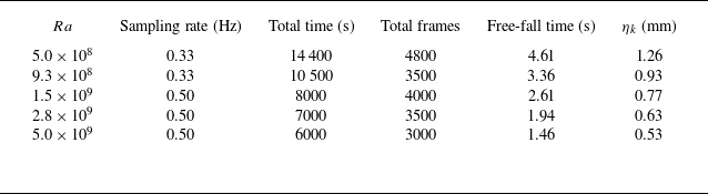
The experimental measurements of the flow field were performed with
 $Ra$
ranging from
 $5.0 \times 10^{8}$
to
 $5.0 \times 10^{9}$
at fixed
 $Pr=5.7$
, which corresponds to average temperature
 $28\,^\circ {\rm C}$
. The related measurement parameters are listed in table 1. During the experiments, the cell is carefully levelled and placed in a room where the temperature is maintained at approximately
 $28\,^\circ {\rm C}$
by an air conditioner.
Parameters for Tomo PIV measurement. Here,
 $\eta _k$
is the Kolmogorov length, which is calculated by
 $\eta _k = Pr^{0.5}/[Ra\, (Nu - 1)]^{1/4}$
, where
 $Nu$
is the dimensionless heat transport, which is measured in our experiments but not reported here.

3. Result and discussion
3.1. Global features of the flow field
Figure 2 illustrates the instantaneous three-dimensional flow fields at five different
 $Ra$
ranging from
 $5.0 \times 10^{8}$
to
 $5.0 \times 10^{9}$
. The flow field is presented by the streamlines of the instantaneous velocity field, and the colour of the streamlines represents both the direction and magnitude of the vertical velocity, with positive (negative) value corresponding to the upward (downward) velocity. While the flow field depicted in figure 2 represents an instantaneous snapshot, it effectively captures the general features of the flow field at different
 $Ra$
. From figures 2(a–e), it is evident that in such a very slender geometry, a distinct single-roll LSC with ascending flow on one side and descending flow on the other side, which is typically observed in a unit cylindrical or rectangular cell (Xia, Sun & Zhou Reference Xia, Sun and Zhou2003; Xi, Lam & Xia Reference Xi, Lam and Xia2004), is absent. Instead, the flow in such a very slender cell appears to be in the helical form at first glance, as the ascending and descending flows undergo azimuthal motion as they travel vertically along the sidewall; one can see an example of this event at approximately the middle height of figure 2(a). While a closer look shows that sometimes the ascending and descending flows can also intersect and cross each other, one can see an example of this event at approximately the bottom of figure 2(a). An overall picture of the flow structure is that the flow is divided into different segments in the vertical direction irrespective of whether the neighbouring segments are divided by a
 $180^\circ$
orientation change of the ascending and descending flows or by an intersect and crossing of the ascending and descending flows. And it is evident that as
 $Ra$
increases, the number of segments gradually increases.
Instantaneous three-dimensional flow fields at five different
 $Ra$
ranging from
 $5.0 \times 10^{8}$
to
 $5.0 \times 10^{9}$
. The flow field is illustrated by the streamlines of the instantaneous velocity field, with the colour indicating both the direction and magnitude of the vertical velocity. Positive values correspond to upward velocity, while negative values correspond to downward velocity.

Log-log plot of
 $Re$
as a function of
 $Ra$
. The slope of the best fitting (blue) line is 0.43. Inset: the same data as in the main plot, but
 $Re$
is compensated by
 $Ra^{0.43}$
.

Figure 3 shows the measured Reynolds number
 $Re$
as a function of
 $Ra$
. Here,
 $Re = UH/\nu$
, where
 $U = \langle u^{2}+v^{2}+w^{2} \rangle _{Vol,t}^{1/2}$
, with
 $\langle \rangle _{Vol,t}$
meaning volume (entire cell) and time (duration of the experiment) average. The scaling of
 $Re$
versus
 $Ra$
is found to follow
 $Re \sim Ra^{0.43}$
. According to the Grossmann–Lohse (GL) theory (Ahlers et al. Reference Ahlers, Grossmann and Lohse2009), the
 $Ra{-}Pr$
space can be categorised into eleven regimes. If we neglect the effect of aspect ratio
 $\Gamma$
, then the parameters of our experiments fall within regime
 $IV_{u}$
. In this regime, GL theory predicts a scaling of
 $Re \sim Ra$
to be
 $4/9$
, which aligns closely with our experimental findings.
In figure 4, we present the horizontal map of the averaged magnitude of the horizontal and vertical velocities for five
 $Ra$
values. Here, the horizontal velocity comprises both
 $u$
and
 $v$
, and the vertical velocity is represented by
 $w$
. The horizontal map is obtained by averaging the velocity over the entire height and time. Due to the thin boundary layer compared to the cell height, averaging over the height primarily reflects the flow state in the bulk region of the cell. The top row of figure 4 depicts the horizontal velocity magnitude. In all cases, this value reaches its maximum at the centre and decreases towards the sidewall, indicating that the most significant horizontal movement occurs in the centre of the domain. The horizontal map of the vertical velocity magnitude is shown in the bottom row of figure 4; the distributions exhibit annulus shapes for relative high
 $Ra$
, such as
 $Ra = 1.5\times 10^{9}$
,
 $2.8\times 10^{9}$
and
 $5\times 10^{9}$
, with equal values in the azimuthal direction. Schmidt et al. (Reference Schmidt, Calzavarini, Lohse, Toschi and Verzicco2012) reported a similar distribution in their simulation with vertically unbounded slender cells, and demonstrated that the position with the maximum value shifts towards the sidewall as
 $Ra$
increases. In our experiments, within the
 $Ra$
range, the position of the maximum value remains almost unchanged, which occurs at approximately
 $2/3$
radius. When
 $Ra$
is small, such as for
 $Ra = 5\times 10^{8}$
and
 $9.3\times 10^{8}$
, unlike the high
 $Ra$
cases, the vertical velocity shows a saddle-shaped distribution, with the maximum values located at two preferred orientation regions, as shown in figures 4(a) and 4(b). The formation of this distribution is because when
 $Ra$
is small, the flow orientation remains relatively steady both in height and over time. There are large and persistent separated ascending and descending flows that have preferred orientations, thus contributing to this distribution. When
 $Ra$
is increased, the ascending and descending flows change their orientations more frequently, and the preference of the orientation disappears. However, this variation does not occur for the horizontal map of the horizontal velocity. It is because, on the one hand, the vertical velocity is the main component of the flow, which can be seen from the magnitude of velocity at figure 4, and on the other hand, the horizontal velocity is naturally small near the sidewall since the horizontal velocity vanishes due to the impenetrable boundary condition at the sidewall.
Horizontal maps of the averaged magnitudes of the horizontal and vertical velocities. Top row: horizontal velocity magnitude (
 $\langle u^{2}+v^{2}\rangle _{V,t}^{1/2}$
). Bottom row: vertical velocity magnitude (
 $\langle w^{2}\rangle _{V,t}^{1/2}$
), where
 $\langle \rangle _{V,t}$
denotes averaging over entire height and time.

3.2. The spatial structure of the flow field
We further discuss the spatial flow structure by examining instantaneous flow fields. We begin with examining the case of small
 $Ra$
. Figure 5(a) presents the instantaneous flow field for
 $Ra=5\times 10^{8}$
, and figure 5(b) displays the horizontal-averaged vertical and horizontal velocities at different heights. It can be seen that at most heights, the vertical velocity significantly exceeds the horizontal component, indicating that the predominant direction of the flow is vertical. However, at
 $0.15H$
, the two curves almost intersect, with the horizontal velocity increasing to a maximum value, and the vertical velocity decreasing to a minimum simultaneously. By looking carefully at the horizontal cross-section of the flow field near
 $0.15H$
, as shown in figure 5(d), it becomes clear that from
 $0.1H$
to
 $0.2H$
, the descending flow (blue region) gradually travels from left to right. Simultaneously, the ascending flow (red region) is squeezed to separate and move towards the sidewall, forming an annulus shape. Eventually, the descending flow moves to the right-hand side, the squeezed ascending flow is re-merged together at the left-hand side, completing an azimuthal positional exchange between the descending and ascending flows. We define this azimuthal positional exchange process due to the intersection and crossing of the ascending and descending flows as a crossing event.
At
 $Ra=5.0 \times 10^{8}$
, (a) streamlines of the instantaneous flow field, and (b) horizontal-averaged vertical and horizontal velocity magnitudes as functions of height, where
 $\langle \rangle _{H}$
represents the average over the horizontal cross-section. (c,d) Horizontal cross-sections of the instantaneous flow field at different heights, corresponding to the twisting and crossing events.

There is another scenario for the azimuthal positional exchange between the descending and ascending flows, as shown in figure 5(c). In this scenario, the ascending and descending flows slowly twist azimuthally, with their shapes and flow strength remaining unchanged. For instance, at
 $0.5H$
, the ascending flow (red region) is situated on the left-hand side. As it ascends, the ascending flow gradually rotates azimuthually in the anticlockwise direction. By the time it reaches
 $0.7H$
, it has rotated azimuthually by almost
 $90^\circ$
. At the same time, the descending flow also rotates azimuthally in the clockwise diretion by about
 $90^\circ$
. From figure 5(b), it can be seen that both the vertical and horizontal velocities do not vary significantly during the event, which distinguishes them from the crossing event. Thus we refer to this behaviour as a twisting event. It should be noted that the azimuthal rotation directions of the flow at different heights are not always the same; for example, from
 $0.85H$
to
 $0.9H$
, the ascending/descending flow rotates in the clockwise direction, while the flow around
 $0.5H$
is rotating in the anticlockwise direction. This implies that the flow cannot be described by a simple helical structure with uni-rotating direction. Given the two events described above, one interesting question arises regarding the number of segments in figure 5(a). At first glance, one might infer that there are four segments, based on the three intersections of the ascending and descending flows in the streamlines. However, it is important to note that a twisting event (such as those at
 $0.6H$
and
 $0.85H$
) does not lead to the formation of a new segment. Only a crossing event can lead to a new segment. Thus there are only two segment in figure 5(a): one is the flow below
 $0.15H$
, and the other is the flow above
 $0.15H$
. Using crossing events to separate different segments of the flow is consistent with the method proposed in Zwirner et al. (Reference Zwirner, Tilgner and Shishkina2020). It should be noted that the two segments divided by the crossing event are very different from two vertically stacked rolls, because the streamlines near the boundary of the two rolls will not intersect; instead, they should be separated and largely parallel to each other. To conclude, the measured three-dimensional flow field reveals that the flow in this very slender cell is neither in a single helical form nor in a multi-roll form.
3.3. Flow mode analysis
To gain further insights into the flow field and also effectively identify the crossing and twisting events, we employ the mode decomposition analyses. By projecting the velocity onto different velocity modes, we can extract quantitative information about the flow field. Previous investigations suggest that typically only a few modes are required to quantitatively describe the essential dynamics of the flow in an RBC cell (Xi et al. Reference Xi, Zhang, Hao and Xia2016; Chen et al. Reference Chen, Huang, Xia and Xi2019).
Given the intricate three-dimensional property of the flow field described above, it is natural to consider using mode decomposition of the three-dimensional velocity field into the three-dimensional modes, as was done in Reiter, Zhang & Shishkina (Reference Reiter, Zhang and Shishkina2022) (see figure 17 in their paper). However, employing three-dimensional modal decomposition requires the flow to be periodic and relatively steady, which contrasts with the results presented in the current study. Thanks to the fact that in our experimental results the vertical velocity in the horizontal cross-sections during the events exhibits simple and characteristic patterns, we are able to conduct the modal analysis for the vertical velocity in the horizontal cross-section at different heights. Here, following the approach outlined by Shishkina (Reference Shishkina2021) and Reiter et al. (Reference Reiter, Zhang and Shishkina2022), we construct two-dimensional flow modes on the horizontal cross-section of the cylinder. This involves utilising Bessel functions in the radial direction and Fourier functions in the azimuthal direction. We then decompose the vertical velocity at each horizontal cross-section of different height into these modes.
(a) Schematic patterns of the five typical modes with azimuthal wavenumbers
 $m=0, 1, 2, 3, 4$
. (b) Height- and time-averaged energy
 $\langle E_{m}\rangle$
contained in the
 $m=0, 1, 2, 3, 4$
modes as functions of
 $Ra$
. The cumulative energy of these modes is also depicted, denoted by orange squares.

The general form of the vertical velocity modes is
 \begin{equation} w_{m}(r,\varphi )=J_{m} ( \widetilde {\alpha _{m}}r/R)\cos (m \varphi ), \end{equation}
where
 $m=0,1,2,3,4$
is the azimuthal wavenumber,
 $w_{m}$
represents the
 $m$
th-order vertical velocity mode,
 $r$
is the radial position,
 $\varphi$
is the azimuthal angle,
 $J_{m}$
represents the
 $m$
th-order Bessel function of the first kind,
 $\widetilde {\alpha _{m}}$
denotes the first positive root of the first derivative of the
 $m$
th-order Bessel function, and
 $R$
is the radius of the cylindrical cell. The patterns corresponding to these five modes (i.e.
 $m=0,1,2,3,4$
) are shown in figure 6(a).
To quantify the contribution of each mode in the flow field, we project the flow field of each horizontal cross-section onto the respective flow modes, and calculate the amplitude
 $A_{m}$
of each mode, which is defined as
 \begin{equation} A_{m}=\int _{S}^{}\frac {w\,w_{m}(\varphi _m)}{\| w_m \| }\,{\rm d}S, \end{equation}
where
 $\| w_m \|$
denotes the magnitude of each mode, calculated as
 $\| w_m \| = w_m w_m^{{\rm T}}$
. For
 $m = 1, 2, 3, 4$
modes, we adopt the largest value of right-hand side of (3.2) as
 $A_{m}$
by altering the azimuthal angle
 $\varphi$
of these modes during the calculation, and the corresponding azimuthal angle is
 $\varphi _m$
. Following previous studies (e.g. Xi et al. Reference Xi, Zhang, Hao and Xia2016), we evaluate the energy contained in the
 $m$
th-order mode
 $E_m$
as
 $E_m = A_m^2 / w^2$
for each horizontal cross-section, where the energy contained in each mode is normalised by the kinetic energy
 $w^2$
of each horizontal cross-section. This normalisation ensures that
 $E_m$
remains within the range 0–1, also facilitating comparisons across different heights and time instants. In figure 6(b), we present the height- and time-averaged energy
 $\langle E_{m}\rangle$
contained in the
 $m=0, 1, 2, 3, 4$
modes as functions of
 $Ra$
, along with their cumulative energy. The height-averaging involves calculating
 $\langle E_m\rangle _H$
by averaging
 $E_m$
across all the horizontal cross-sections within a single instantaneous snapshot, yielding one value for each time instant. By time-averaging the time series of these instantaneous
 $\langle E_m\rangle _H$
, we obtain the height- and time-averaged energy
 $\langle E_{m}\rangle$
of each mode. It is seen that these five modes account for over
 $80\,\%$
of the total energy within the current
 $Ra$
range. The
 $m = 1$
(first-order) mode dominates the flow field, while the energy contributions from the
 $m = 3$
and
 $m = 4$
modes are negligibly small across the entire range of
 $Ra$
. As
 $Ra$
increases, the energy contained in the first-order mode decreases, whereas the energy contained in the
 $m = 0$
(zeroth-order) mode increases. Meanwhile, the energy contained in
 $m = 2$
(second-order) mode remains relatively constant and smaller than that of the zeroth-order mode. Although the energy in the second-order mode is comparable to that of the zeroth-order mode, the zeroth-order mode exhibits a stronger correlation with the crossing events discussed earlier. Specifically, during the crossing events, the energy contained in the zeroth-order mode can even surpass that of the first-order mode, as we will demonstrate below. Therefore, to simplify the subsequent analysis, we will focus our discussion on the zeroth- and first-order modes exclusively. We have to emphasise that we conduct the modal analysis for the vertical velocity in the horizontal cross-section at different heights. So actually, these modes represent the vertical flow, not the horizontal flow. Through examining the amplitude/energy content of each mode at different heights, we can see how the vertical flow varies in the vertical direction.
At
 $Ra=5.0 \times 10^{8}$
, for the same velocity field as shown in figure 5: (a) streamlines and horizontal cross-sections of the instantaneous flow field; (b) horizontal-averaged vertical and horizontal velocity magnitudes as functions of height, it is replotted here for better comparison; (c) energy contained in the
 $m=0$
and
 $m=1$
modes as functions of height; (d) variation of azimuthal angle of the
 $m=1$
mode with height.

Figure 7(c) shows the energy
 $E_m$
contained in these two modes at different heights for
 $Ra=5.0 \times 10^{8}$
. It is evident that at most heights, the energy contained in first-order mode is larger than that of the zeroth mode, suggesting that the dominant flow pattern in the cell is represented by ascending flow on one side, and descending flow on the other side. Upon comparing with the velocity magnitude profiles shown in figure 7(b), it is apparent that in the region where the first mode dominates, the magnitude of vertical velocity increases continuously, and reaches its maximum at approximately the middle height of the cell. Conversely, when the zeroth mode dominates, the magnitude of vertical velocity decreases, while the magnitude of horizontal velocity increases. Furthermore, it is found that, inside a crossing event at approximately
 $0.15H$
, the energy contained in the zeroth mode significantly increases and surpasses that of the first mode. Such evolution of zeroth and first mode with height can be used to identify the crossing event. Thus practically, we define a crossing event where the energy contained in the zeroth mode exceeds that of the first mode. We further verified that relaxing the criterion does not affect the experimental results (see Appendix A).
Given that the first mode is dominant in most of the height, its azimuthal angle can approximately represent the corresponding orientation of the flow at different heights. Figure 7(d) depicts the variation of the flow orientation with height. It can be observed that when a crossing event occurs, the orientation of flow field suddenly changes by
 $180^\circ$
within a very short vertical distance. In contrast, a twisting event results in continuous changes in orientation with height over the range of
 $0.4H$
to the top plate. Our measurements reveal that the rotating direction, the duration of a continuous rotation and the maximum rotation angle during the twisting event are all in a random manner. Furthermore, between
 $0.18H$
and
 $0.44H$
, the orientation of the flow remains unchanged, indicating a very stable non-twisting roll-like flow structure.
At
 $Ra=5 \times 10^{9}$
: (a) streamlines and horizontal cross-sections of the instantaneous flow field; (b) horizontal-averaged vertical and horizontal velocity magnitudes as functions of height; (c) energy contained in the
 $m=0$
and
 $m=1$
modes as functions of height; (d) variation of azimuthal angle of the
 $m=1$
mode with height.

As
 $Ra$
increases, the flow field experiences more crossing and twisting events. Figures 8(a) and 8(c) show the instantaneous flow field at
 $Ra=5\times 10^{9}$
and the energy contained in the two dominant flow modes. Similar to the low
 $Ra$
case, the first mode dominates at most of the heights, while the energy contained in the zeroth mode surpasses that of the first mode at four heights where the crossing occurs. We note that at higher
 $Ra$
cases, the surpassing might not be as pronounced as that in relative lower
 $Ra$
. This is because the crossing event is not only the spatial feature of the flow field, but also a dynamic feature evolving with time. It is very likely that these moments are just before or after a crossing event in time. Or it could well be the case that the energy contained in the zeroth-order mode approaches, but eventually does not exceed that of the first-order mode. In current measurements, the sampling frequency is relatively slow, which may be not sufficient to capture all the instantaneous turbulent features, especially at high
 $Ra$
with smaller characteristic time scale. However, in general, the crossing event occurs more frequently at high
 $Ra$
, as shown in figure 8 compared to low
 $Ra$
. Furthermore, in the higher
 $Ra$
case, the orientation of the flow changes more rapidly, as can be seen in figure 8(d), which indicates that the twisting event also occurs more frequently. The presence of a large and stable roll-like flow structure with fixed orientation is hardly observed, which is evident from the velocity magnitudes and the energy shown in figures 8(b) and 8(c).
At
 $Ra=9.3 \times 10^{8}$
: (a) streamlines and horizontal cross-sections of the instantaneous flow field; (b) horizontal-averaged vertical and horizontal velocity magnitudes as functions of height; (c) energy contained in the
 $m=0$
and
 $m=1$
modes as functions of height; (d) variation of azimuthal angle of the
 $m=1$
mode with height.

In addition to the previous findings, one can also see that in figures 7(c) and 8(c), near the boundaries, the zeroth-order mode dominates the flow field. This dominance of the zeroth-order mode can occur over short segments, as seen in top and bottom boundaries of figures 7(c) and 8(c), or it can extend over longer segments, as shown in figure 9(c). In figure 9, we show a typical instantaneous snapshot illustrating long-range dominance of the zeroth-order mode near both the top and bottom boundaries at
 $Ra = 9.3 \times 10^{8}$
. Upon closer examination of the flow field near the bottom boundaries, we find that such a long segment extends to nearly
 $0.2H$
, and the flow field exhibits a donut like structure (see the horizontal cross-sections). This donut like flow structure near the boundaries can be described as follows: the ascending/descending flow emerges and moves upwards/downwards near the sidewall, while the descending/ascending flow moves downwards/upwards along the (radial) centre of the cell until it reaches and impinges upon the plate, thus the annulus is formed. In figure 9(b), we observed that although the zeroth-order mode dominates the flow field similar to that in a crossing event, there are only small changes in the magnitude of both the vertical and horizontal velocities, which distinguishes it significantly from the behaviour inside a crossing event. It should be noted that such donut like flow structure was also reported by Hartmann et al. (Reference Hartmann, Chong, Stevens, Verzicco and Lohse2021) in their
 $\Gamma = 1/10$
cylindrical cell by DNS. Practically, we propose a threshold to identify the donut like structure, that is, if the prevalence of the zeroth mode over the first mode lasts for an extended length in the vertical direction (say, longer than
 $0.05H$
) near the boundaries. It is important to emphasise that the donut like flow structure is found exclusively near the boundaries and is almost absent in the bulk region. Additionally, we found that the transition from the donut like flow structure to the roll-like flow structure occurs when the energy contained in the first-order mode exceeds that in the zeroth-order mode, which aligns with the characteristics of a crossing event. Therefore, for clarity, this flow event can also be referred to as a crossing event.
Spatio-temporal evolution of the nodes and their corresponding PDFs. Each blue point represents a node. Here, (a)
 $Ra = 5.0 \times 10^{8}$
, (b)
 $Ra = 9.3 \times 10^{8}$
, (c)
 $Ra = 1.5 \times 10^{9}$
, (d)
 $Ra = 2.8 \times 10^{9}$
, (e)
 $Ra = 5 \times 10^{9}$
. Additionally, in (a), the five dashed lines correspond to the five time points at which the instantaneous flow field is shown in figure 11.

3.4. Temporal and spatial evolution of segments
Let us now discuss the spatio-temporal behaviour of the flow structure, especially focusing on the behaviour of the segment. Based on the results above, here, we divide the flow into segments, where each segment represents the flow portion between two successive crossing events. These segments can manifest as either roll-like flow structures (twisted or non-twisted) or donut like flow structures. To study the length of the segments and its evolution, we define the node separating two successive segments, which is the height where the zeroth mode reaches a local maximum, or the intersection point of the zeroth and first mode when a donut like structure exists near the boundaries. In our experiment, due to the small velocity magnitude near the top and bottom boundaries, we propose setting a threshold
 $0.05H$
; segments shorter than the threshold are not identified.
Figure 10 shows a spatio-temporal evolution of nodes at different
 $Ra$
over 2000 s. Since we set the threshold
 $0.05H$
, there are no nodes within the region comprising
 $5\,\%$
of the total height below the top, and
 $5\,\%$
above the bottom. It can be seen that when
 $Ra = 5.0 \times 10^{8}$
and
 $ 9.3 \times 10^{8}$
, the number of the nodes is relative small, and they are mostly concentrated in the regions close to the top and bottom boundaries. From figure 10(a), it is evident that the segments near the bottom grow in length over time. In figures 11(a–d), we present the four instantaneous snapshots near the bottom boundary at four different time points, as labelled in figure 10(a). Over time, the height of the two nodes gradually increases, as shown by the dashed lines. Specifically, the lower segment grows in length, while the upper segment decreases in length. It appears that a cap prevents the lower segments from growing freely or exceeding this cap, which is located at approximately
 $0.4H$
. At certain time points (see figure 11
e), when the segments near the boundaries reach the cap at approximately
 $0.4H$
, they suddenly collapse and the nodes disappear. Unlike the continuous growth of segments from the bottom, the segments near the top boundary stay relatively unchanged in length, showing an asymmetry in the flow structure. Such an asymmetry in slender cells has been reported previously by Hartmann et al. (Reference Hartmann, Chong, Stevens, Verzicco and Lohse2021); they reported an asymmetric temperature distribution with height, through DNS with a
 $\Gamma =0.1$
cylindrical cell. They conjectured that such an asymmetric behaviour is related to the existence of a lower sublayer. Obviously, further understanding is required to elucidate the reasons for this asymmetry. For
 $Ra=9.3 \times 10^{8}$
, figure 10(b) exhibits relative symmetric distribution of the nodes. These nodes disappear at approximately
 $0.2H$
away from both top and bottom plates. A common feature of the first two low
 $Ra$
cases is that the bulk region has fewer nodes. The middle parts of both figures 10(a) and10(b) are relatively blank, indicating that longer segments can exist in the bulk. When
 $Ra$
is larger, the bulk region starts to exhibit more nodes, as shown in figure 10(c) for
 $Ra=1.5 \times 10^{9}$
, while for
 $Ra=2.8 \times 10^{9}$
and
 $5 \times 10^{9}$
, the entire height of the cell is filled with nodes, indicating that the crossing event occurs more uniformly at all heights. This suggests that the flow enters a more chaotic state, especially for the bulk region.
Instantaneous three-dimensional flow field near the bottom boundary at the five different time points, corresponding to the dashed lines labelled a–e in figure 10(a). The flow field is visualised using streamlines of the instantaneous velocity field, with colour coding to represent both the direction and magnitude of the vertical velocity. Positive values indicate upward velocity, whereas negative values indicate downward velocity. The two dashed lines depict the tracks of the two nodes.

Time evolution of the azimuthal angle of the
 $m=1$
mode at middle height for five different
 $Ra$
over 2000 s: (a)
 $Ra = 5.0 \times 10^{8}$
, (b)
 $Ra = 9.3 \times 10^{8}$
, (c)
 $Ra = 1.5 \times 10^{9}$
, (d)
 $Ra = 2.8 \times 10^{9}$
, (e)
 $Ra = 5 \times 10^{9}$
.

On the right-hand side of figure 10, we present the probability density functions (PDFs) of the heights where the nodes are located for five different
 $Ra$
values. For all
 $Ra$
, the PDF has a larger value near the boundaries, which indicates that the regions near boundaries have more nodes, i.e. more crossing events. The PDF in the bulk region is relatively flat, indicating no significant preference for the occurrence of crossing events at specific heights in the bulk region. As
 $Ra$
increases, the peak value of the PDF near the boundaries decreases, suggesting that more crossing events occur in the bulk region, indicating a more uniform distribution of crossing events across all heights.
In figure 12, we present the time evolution of the flow orientation (the azimuthal angle of the first-order mode) at middle height for five different
 $Ra$
values. For
 $Ra=5.0 \times 10^{8}$
and
 $9.3 \times 10^{8}$
, the orientation changes in only a very limited range. For
 $Ra=1.5 \times 10^{9}$
, the flow orientation at middle height starts continuous rotating but with no preferred direction. For
 $Ra=2.8 \times 10^{9}$
and
 $ 5 \times 10^{9}$
, the continuous rotating becomes much more rapid, and the rotating range becomes much larger, and this indicates a more chaotic state of the flow.
The PDFs of (a) segment number, and (b) segment length, for the five different
 $Ra$
values.

Finally, we discuss the statistics of flow segments. Figure 13 presents the PDFs of segment number and segment length for different
 $Ra$
values. In figure 13(a), it is evident that as
 $Ra$
increases, the most probable segment number rises slightly, from approximately 2 to 4, with the peak probability decreasing from nearly 0.5 to approximately 0.3. At
 $Ra = 5.0 \times 10^8$
, the peak heights for segment numbers 2 and 3 are comparable. For
 $Ra = 9.3 \times 10^8$
and
 $Ra = 1.5 \times 10^9$
, the PDFs are quite pronounced, with the peak located at segment number 3. As
 $Ra$
continues to increase, the PDFs broaden, and the peak segment number gradually shifts higher. For example, at
 $Ra = 5.0 \times 10^9$
, 5–6 segments within the cell are frequently observed, as indicated by the PDF. Figure 13(b) shows the PDFs of segments length at five different
 $Ra$
values. For
 $Ra \leqslant 1.5\times 10^{9}$
, the PDF distribution can be interpreted as having two peaks: one peak corresponds to a longer segment, typically between
 $0.5H$
and
 $0.7H$
, while the other peak is associated with a shorter segment at approximately
 $0.1H$
. When
 $Ra \gt 2.8 \times 10^{9}$
, only shorter segments dominate, with peaks of segment lengths approximately
 $0.1H$
. One may wonder why the most probable segment length is only
 $0.1H$
when the most probable segment number is 4 at
 $Ra = 5.0 \times 10^9$
. This is reasonable since the segments are not equal sized. For example, there can be four segments, with three of them having length approximately
 $0.1H$
, and the other segment having length approximately
 $0.7H$
. Regarding the peak located at approximately
 $0.1H$
observed in all cases with varying
 $Ra$
, it implies that segments with equal length and width have a high probability of forming within the cell. According to Zwirner et al. (Reference Zwirner, Tilgner and Shishkina2020), mode transitions between multiple-roll states in a
 $\Gamma = 0.2$
cell are driven by the elliptical instability. For an elongated segment present in our experiments – such as the long segment above
 $0.15H$
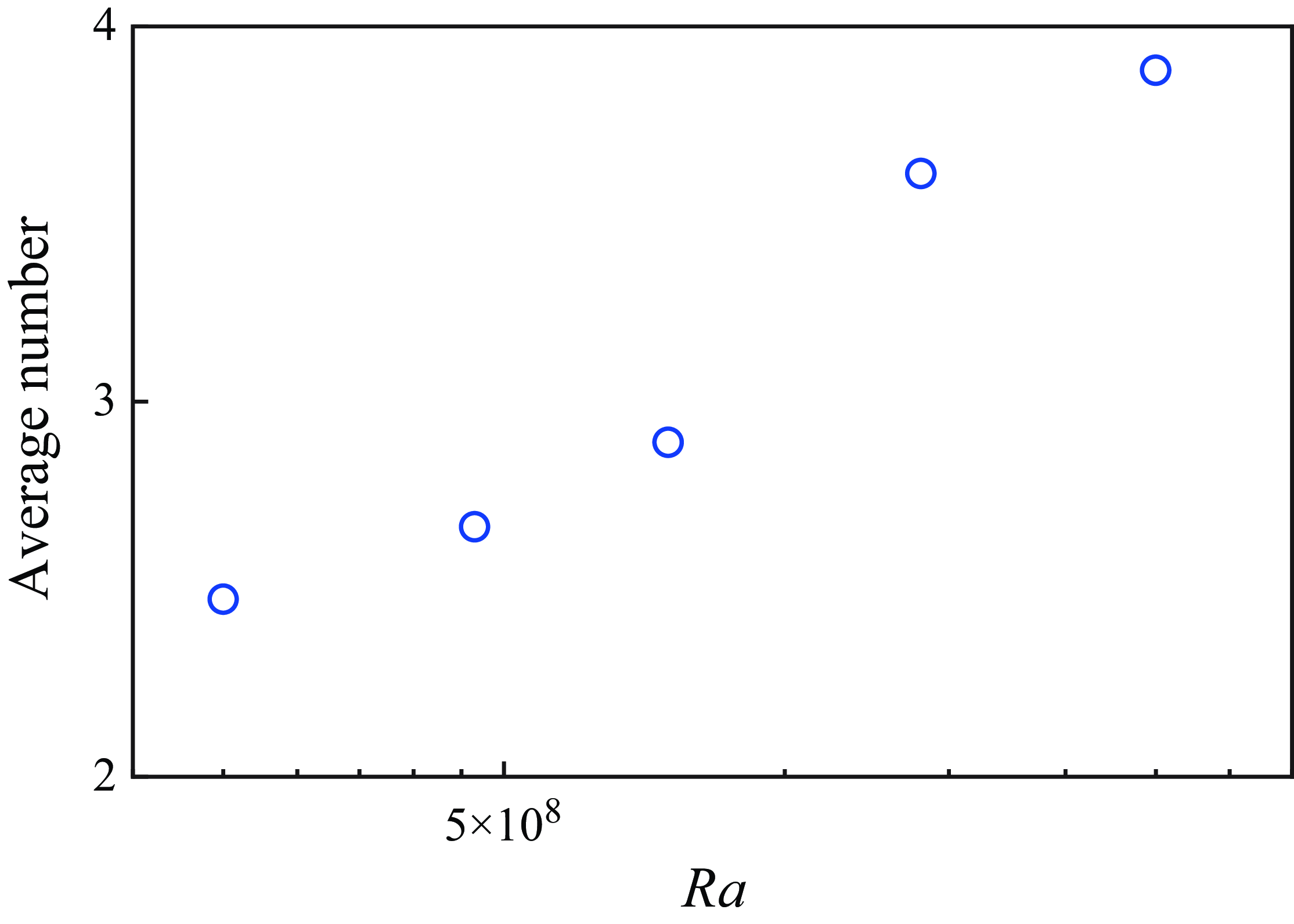
shown in figure 5 – this elliptical instability presumably triggers its break-up, leading to the emergence of multiple-segment flow modes. Additionally, Zwirner et al. (Reference Zwirner, Tilgner and Shishkina2020) highlighted the role of prominent azimuthal flow during the break-up process, suggesting that such azimuthal motion can twist or disrupt single-roll flows. In our paper, we also illustrate twisting events at various heights through mode decomposition. Due to the elliptical instability, longer segments are likely to break into shorter ones. This instability-driven break-up process is constrained by a limit, where the roll/segment achieves a configuration with equal length and width (Waleffe Reference Waleffe1990). In figure 14, we display the average number of segments as a function of
 $Ra$
. One can see that the average number of segments increases with
 $Ra$
. This trend is consistent with the results presented in figure 13 and in figure 2.
The average number of segments as a function of
 $Ra$
.

4. Conclusion
In summary, we have conducted an experimental study of the three-dimensional flow structure inside a very slender cylindrical cell with
 $\Gamma = 1/10$
by using Tomo PIV. Our experiments reveal that the flow structure within this very slender cell is not in the single-roll form. Instead, the ascending and descending flows can intersect and cross each other, resulting in the crossing event. These crossing events separate the flow into segments in the vertical direction. Within each segment, the ascending and descending flows ascend or descend side by side vertically or in a twisting manner, and the twisting is not unidirectional, while the segments near the boundary can also be in the form of a donut like structure. During a crossing event, the azimuthal position exchange between ascending and descending flows is accomplished by the ascending/descending flow travelling horizontally and crossing the descending/ascending flow. The twisting event involves azimuthal rotation of the ascending and descending flows along the cell axis without significant changes in flow strength. By employing the mode decomposition analyses, we quantitatively describe the instantaneous flow field and hence identify the crossing events as well as the twisting events. The most important modes in the slender cell are the first mode, where the ascending and descending flows are located at the two ends of the diameter of the cylindrical cell, and the zeroth mode, where the ascending/descending flow is inside the descending/ascending flow, i.e. the annulus mode. Our results indicate that a crossing event occurs when the energy contained in the axisymmetric (zeroth-order) mode increases, and the energy contained in the diametrically antisymmetric (first-order) mode decreases. With the increase of
 $Ra$
, the crossing event occurs more frequently. The variation of the azimuthal angle of the first mode with height provides insights into the twisting event, i.e. the gradual reorientation of the helical flow. At lower
 $Ra$
cases, the helical flow reorientates in a limited azimuthal range, while for higher
 $Ra$
cases, it shows rapid and continuous azimuthal rotation in a broader azimuthal range, indicating a more chaotic flow state. Statistical analysis of the modes reveals that as
 $Ra$
increases, the average length of the segments becomes smaller, and the average number of segments increases from 2.5 to 3.9 in the
 $Ra$
range of our experiments.
We are now well-positioned to review the three major numerical studies (Iyer et al. Reference Iyer, Scheel, Schumacher and Sreenivasan2020; Zwirner et al. Reference Zwirner, Tilgner and Shishkina2020; Hartmann et al. Reference Hartmann, Chong, Stevens, Verzicco and Lohse2021) in light of our experimental results. In particular, as simulations of Hartmann et al. (Reference Hartmann, Chong, Stevens, Verzicco and Lohse2021) are in
 $Ra$
and
 $Pr$
ranges similar to those in our experiments (their simulations use
 $10^7 \leqslant Ra \leqslant 10^{10}$
,
 $Pr = 4.38$
; our experiments use
 $5\times 10^8 \leqslant Ra \leqslant 5\times 10^9$
,
 $Pr=5.7$
), we compared in detail our experimental results with their simulation data (we obtained the data through private communication with the first author of Hartmann et al. Reference Hartmann, Chong, Stevens, Verzicco and Lohse2021). For the flow field of Hartmann et al. (Reference Hartmann, Chong, Stevens, Verzicco and Lohse2021) at small
 $Ra$
, the flow structure is similar to ours, where the ascending and descending flows travel vertically along the sidewall, with crossing events and twisting events occurring at some heights. When
 $Ra$
gets higher, both crossing events and twisting events become more pronounced, consistent with our experimental observations. Based on the detailed comparison, we find that our experiments and their simulations are consistent with each other. Regarding the other two major studies, we must emphasise that the parameter ranges in our experiments do not fully overlap with theirs, particularly in terms of variations of
 $Pr$
, making direct comparisons inappropriate. Zwirner et al. (Reference Zwirner, Tilgner and Shishkina2020) suggested the presence of multiple rolls stacked on top of each other in the parameter regime
 $Ra = 5 \times 10^5$
and
 $Pr = 0.1$
. However, upon closer inspection, the flow fields also exhibit crossing events similar to those observed in our study, particularly in states with more than two rolls (see figures 1(b–d) in Zwirner et al. Reference Zwirner, Tilgner and Shishkina2020), i.e. the stacked rolls are separated by the crossing event that we described here, while the twisting event is observed only in figure 1(a) (single-roll state) of Zwirner et al. (Reference Zwirner, Tilgner and Shishkina2020). This specific case involves a longer roll (in the vertical direction), making the azimuthal motion of the ascending and descending plumes more pronounced. In the multiple-roll cases, where the length of the rolls is shorter, the azimuthal motion is less distinct. Despite these similarities, there is also a significant difference between their results and ours. Notably, in the multiple-roll state (figures 1(b–d) in Zwirner et al. Reference Zwirner, Tilgner and Shishkina2020), the lengths of the rolls are more or less the same. In contrast, our experimental results show that the segment lengths exhibit a wide distribution (see figure 13
b), highlighting the key distinction between the two studies. As for the numerical results by Iyer et al. (Reference Iyer, Scheel, Schumacher and Sreenivasan2020), they attributed the flow field to robust helical flow across the range
 $10^8 \leqslant Ra \leqslant 10^{15}$
, which encompasses our
 $Ra$
range but with a lower
 $Pr = 1$
. Their helical flow can be considered as the twisting event that we reported, but in their case, the twisting occurs consistently in one direction. This differs from our findings, where the twisting is not unidirectional.
To conclude, through our careful experimental analysis, we are able to give a unified description of the flow, i.e. the flow is neither in the multiple-roll form nor in the simple helical form; instead, the ascending and descending flows can intersect and cross each other, resulting in the crossing events. These crossing events separate the flow into segments; within each segment, the ascending and descending flows ascend or descend side by side vertically or in the twisting manner, and the twisting is not unidirectional. Although the flow structures shown in the three major simulations appear very different, we found that these simulation results do share some common features, such as the crossing and twisting events. In spite of the common features, there are indeed some discrepancies, such as spatial distribution of the crossing events, and the direction of the twisting events. The discrepancies might be attributed to the effects of different
 $Pr$
.
Acknowledgements
We are grateful to O. Shishkina, Y.-C. Xie and L. Zhang for stimulating discussions. We thank R. Hartmann and K.L. Chong for sharing with us their simulation data.
Funding
This work was supported by the National Natural Science Foundation of China (NSFC) under grant nos 12125204 and 12388101, the China Postdoctoral Science Foundation under grant nos 2021M702077 and 2022M721854, and the 111 project of China (no. B17037).
Declaration of interests
The authors report no conflict of interest.
Appendix A. Uncertainty of the crossing events identification
To examine the uncertainty on the identification of the crossing events, we compared the statistics of the crossing events obtained through slightly different criteria. In figure 15, we present the results from two slightly different criteria: one with a more relaxed criterion (case A), and another with a more rigorous criterion (case B). For case A, a crossing event is identified even if the energy contained in the
 $m = 0$
mode does not exceed that in the
 $m = 1$
mode but the energies contained in these two modes are quite close, with a difference of no more than
 $5\,\%$
. For case B, a crossing event is identified only if the energy contained in the
 $m = 0$
mode exceeds that in the
 $m = 1$
mode, with a difference greater than
 $5\,\%$
. As shown in figure 15, the results from these two criteria closely align with results obtained from the original criterion (as those presented in figure 13). All data points and lines collapse together, indicating that the slightly different criteria do not significantly affect the overall results.
The PDFs of (a) segment number, and (b) segment length, for the five different
 $Ra$
values, evaluated using three different criteria.

Appendix B. Identify the crossing events with
 $m = 2$
mode included

At
 $Ra = 5 \times 10^9$
: (a) horizontal cross-sections of the instantaneous flow field; (b) horizontal-averaged vertical and horizontal velocity magnitudes as functions of height; (c) energy contained in the
 $m = 0$
,
 $m = 1$
and
 $m = 2$
modes, as functions of height.

To check the effects of the
 $m = 2$
mode on the identification of the crossing events, we have conducted a test to identify the crossing event by taking the
 $m = 2$
mode into account. By including the
 $m = 2$
mode, the total energy of the flow modes used to describe the flow field exceeds 80
 $\%$
. First, in figure 16, we present a typical instantaneous snapshot in which the energy contained in the
 $m = 2$
mode significantly surpasses that of the other two modes in the height range between
 $0.7H$
and
 $0.8H$
. By examining the horizontal cross-sections before and after this range, one can see that as the descending flow travels horizontally and crosses the ascending flow, the ascending flow is split into two parts and is pushed towards the sidewall. This interaction results in a cross-shaped flow structure (
 $z/H \approx 0.75$
) rather than the annular form associated with the
 $m = 0$
mode. The dominance of the
 $m = 2$
mode over the
 $m = 1$
mode can also be interpreted as a type of crossing event. Based on this observation, and in order to include the
 $m = 2$
mode, we revised our crossing event identification criteria for this test. Specifically, a crossing event is now identified if the energy contained in the
 $m = 0$
mode, the
 $m = 2$
mode, or the sum of these two modes, exceeds that contained in the
 $m = 1$
mode. With this new criterion, the PDFs of segment numbers for all five
 $Ra$
cases shift towards higher segment numbers, as shown in figure 17(a). This result is expected, as the inclusion of the
 $m = 2$
mode introduces additional crossing events. Despite this slight shift in the PDF of segment numbers, the trend of increasing segment number with
 $Ra$
remains robust, indicating that our conclusion regarding the relationship between segment number and
 $Ra$
is unaffected by the inclusion of the
 $m = 2$
mode. For the PDFs of normalised segment lengths, as shown in figure 17(b), the distributions remain nearly identical around the first peak between the original criterion and the new criterion with the
 $m = 2$
mode included. However, the tails of the PDFs at larger segment lengths, particularly for higher
 $Ra$
, exhibit small differences. With the new criterion, the probability of having longer segments decreases. This outcome is reasonable because the total number of segments increases with the new criterion, leading to a corresponding reduction in the length of the longer segments.
The PDFs of (a) segment number, and (b) segment length for the five different
 $Ra$
values. The blue circle represents the original method by considering only
 $m = 0$
and
 $m = 1$
modes; the red circle represents the method that considers
 $m = 0$
,
 $m = 1$
and
 $m = 2$
modes.

To conclude, by including the
 $m = 2$
mode, although the PDFs of segment number and segment length differ slightly from those of the original criterion, the overall understanding regarding the statistics of segments remains largely unaffected.