

Residentially mobile hunter-gatherers commonly use a camp for a few days at a time but sometimes weeks or months (Binford Reference Binford1983; Kelly Reference Kelly2013). These camps are central places for foraging trips and provide shelter from the elements and predators and a place to manufacture tools, sleep, cook food, share information and resources, conduct household tasks, and raise offspring. The human species spent much of its evolutionary history as mobile hunter-gatherers (McCall Reference McCall2015; Robinson Reference Robinson, Cummings, Jordan and Zvelebil2014; Ulijaszek et al. Reference Ulijaszek, Mann and Elton2012), so short-term residential camps have been a focal point of human social and economic life for millennia, likely playing an important role in human social evolution (Wiessner Reference Wiessner2014; Wrangham Reference Wrangham2009). The dynamics of hunter-gatherer camps and annual settlement patterns, however, are far from simple. Residence times vary widely, and coresidence patterns of individuals and families within camps are highly fluid (Dyble et al. Reference Dyble, Salali, Chaudhary, Page, Smith, Thompson, Vinicius, Mace and Migliano2015; Hill et al. Reference Hill, Walker, Božičević, Eder, Headland, Hewlett, Hurtado, Marlowe, Wiessner and Wood2011). Yet there are also remarkable consistencies in hunter-gatherer social structures; importantly, group sizes are surprisingly consistent across hierarchical levels of aggregation, independent of environmental variation (Binford Reference Binford2001; Grove et al. Reference Grove, Pearce and Dunbar2012; Hamilton, Milne, Walker, Burger, and Brown Reference Hamilton, Milne, Walker, Burger and Brown2007; see Hill et al. Reference Hill, Bentley and Dunbar2008 and Zhou et al. Reference Zhou, Sornette, Hill and Dunbar2005). A complex fission-fusion dynamic among individuals, families, and bands allows for the flow of social and biological information within dispersed, low-density populations, thus maintaining the ecological, demographic, and economic viability of foraging populations in heterogeneous and often unpredictable environments (e.g., Grueter et al. Reference Grueter, Chapais and Zinner2012; Lévi-Strauss Reference Lévi-Strauss, Bell, von Sturmer and Needham1969; Whallon et al. Reference Whallon, Lovis and Hitchcock2011). Thus, hunter-gatherer populations are well defined as hierarchical, spatially structured metapopulations (Berndt and Berndt Reference Berndt and Berndt1988; Chapais Reference Chapais2008; Hamilton et al. Reference Hamilton, Burger, DeLong, Walker, Moses and Brown2009; Hamilton, Milne, Walker, Burger, and Brown Reference Hamilton, Milne, Walker, Burger and Brown2007; Rodseth Reference Rodseth2012; Rodseth et al. Reference Rodseth, Wrangham, Harrigan and Smuts1991), but research devoted to the structure of the residential camps they form has been limited.
Inferences about mobility and group size from the archaeological record are integral to understanding the evolution of foraging behavior and social structure. In this article, we consider the spatiotemporal dynamics of hunter-gatherer camps. Given that hunter-gatherer populations have a consistent organizational structure, and a predictable set of responses to variation in environmental productivity, here we examine how the structure and dynamics of hunter-gatherer camps vary in response to group size, residence time, and habitat.
We focus on the statistics of ethnoarchaeologically recorded hunter-gatherer camps and compare them with the statistics of ethnographically recorded bands. Our analysis proceeds in two stages: First, we consider the overall scale of hunter-gatherer camps, measured statistically as their average size, structure, and organization. The average emerges from general sets of internal and external constraints interacting to set the overall scale of bands, camps, and their organization. The question is: Do large-scale generalizations about hunter-gatherer groups and their dynamics hold across different groups, regions, or habitats, or do these generalizations break down at finer scales?
Second, we consider variation in the size, structure, and organization of hunter-gatherer camps. The variation emerges from local sets of dynamics acting on individual camps themselves, resulting in departures of each camp from the average behavior. The question here is: How do these dynamics cause patterned deviations from the mean, resulting in the variation we see in data?
Hunter-Gatherer Social Structure and Spatial Ecology
Given their central role in foraging socioeconomies, the size, structure, and dynamics of bands play prominent roles in hunter-gatherer studies, both archaeologically and ethnographically (e.g., Binford Reference Binford1978, Reference Binford1983; Gould Reference Gould1978; Hamilton, Milne, Walker, Burger, and Brown Reference Hamilton, Milne, Walker, Burger and Brown2007; Hassan Reference Hassan1981; Lee and DeVore Reference Lee and DeVore1968; Yellen Reference Yellen1977; see Kelly Reference Kelly2013 and references therein). Anthropologists debated “band” social structure (e.g., Radcliffe-Brown Reference Radcliffe-Brown1930; Steward Reference Steward1936, Reference Steward1938) but assumed that membership was rigid. However, in the 1960s and 1970s, detailed ethnographic studies showed that bands, even if bounded in space, had fluid, not rigid, membership (Lee Reference Lee1979; Yellen Reference Yellen1977). Bands also had a finite longevity, retaining an individual identity for several years but eventually reforming into new bands with new identities. For example, in his study of the Dobe !Kung, between 1962 and 1972, Lee (Reference Lee1979) recorded that out of 16 original study groups, six had disbanded. Moreover, while foraging bands often spend much of the year operating as individual economic units, they regularly coalesce, sometimes for extended periods of time: for example, Australian Aborigines (Berndt and Berndt Reference Berndt and Berndt1988), Netsilik (Balikci Reference Balikci1970), Beaver (Brody Reference Brody1981), Inupiaq (Burch Reference Burch2006), Cheyenne (Grinnell Reference Grinnell1972), Sioux (Hassrick Reference Hassrick1964), Kaingang (Henry Reference Henry1964), Dobe !Kung (Lee Reference Lee1979), Hadza (Marlowe 2012), Chiricahua Apache (Opler Reference Opler1941), Nukak (Politis Reference Politis2009), and !Kung (Yellen Reference Yellen1977). Often these periodic aggregations occur seasonally. In some cases, the opposite occurs, and bands split into individual families, operating as independent economic units for extended periods of time, frequently in response to extreme aridity: for example, the G/wi, !Xo, /Xam, G//ana (Barnard Reference Barnard1992), and Ngadadjara (Gould Reference Gould1978).
Since the “Man the Hunter” conference in 1966 (Lee and DeVore Reference Lee and DeVore1968), anthropological lore has held that foraging bands are made up of about 25 individuals (Birdsell Reference Birdsell, Lee and DeVore1968). However, the “magic number” of 25 in “Man the Hunter” was neither dogmatic nor defended, and empirical support for it is questionable (Kelly Reference Kelly2013). More recent theories propose constraints on hunter-gatherer group size such as nutritional limits to maintaining aggregations of human foraging groups (Lieberman Reference Lieberman2013), the reduction of variance in postsharing return rates (Kelly Reference Kelly2013), compounding political stress in social groups (Johnson Reference Johnson, Renfrew, Rowlands and Segraves-Whallon1982), and cognitive limits to social interactions (Dunbar Reference Dunbar2003; Dunbar and Shultz Reference Dunbar and Shultz2007).
Using Binford's (Reference Binford2001) large, cross-cultural database of ethnographic and ethnohistoric foraging societies, Hamilton, Milne, Walker, Burger, and Brown (Reference Hamilton, Milne, Walker, Burger and Brown2007) show that foraging populations are structurally hierarchical, modular, and statistically self-similar. Each structural level of social organization, from families and bands, macrobands, and regional aggregations to total populations, are simply groups of lower-level aggregations, with a constant branching rate of approximately three to four (see also Zhou et al. Reference Zhou, Sornette, Hill and Dunbar2005). Importantly, and somewhat surprisingly, the sizes of these aggregations and the statistical structure of the metapopulations they form are invariant across environments.
Yet, despite the consistent organizational structure of bands, hunter-gatherer spatial ecology varies widely across different environments (Binford Reference Binford2001; Kelly Reference Kelly2013). In fact, the size of hunter-gatherer home ranges varies predictably with energy availability, modeled as environmental productivity (Hamilton, Milne, Walker, and Brown Reference Hamilton, Milne, Walker, Burger and Brown2007). A simple model of ecosystem energetics predicts variation in energy-dependent spatial requirements, and Arctic foragers require areas orders of magnitude greater than do tropical hunter-gatherers due to differences in energy availability (and predictability). Hunter-gatherer populations also exhibit economies of scale in space use across these same environments: larger populations require decreasing amounts of space per individual to meet their metabolic requirements (Hamilton, Milne, Walker, and Brown Reference Hamilton, Milne, Walker and Brown2007). This occurs, presumably, due to increasing returns to scale of cooperation and information sharing between individuals connected by extensive social networks (Hamilton et al. Reference Hamilton, Burger, DeLong, Walker, Moses and Brown2009). Similar patterns are also observed in a range of subsistence-level agricultural societies (e.g., Freeman et al. Reference Freeman, Byers, Robinson and Kelly2018; Hamilton et al. Reference Hamilton, Buchanan, Huckell, Holliday, Shackley and Hill2013). Subsequent work has shown the same ecological dependency in rates of hunter-gatherer residential mobility (Grove Reference Grove2009; Hamilton et al. Reference Hamilton, Lobo, Youn, Rupley and West2016). In these studies, variation in rates of residential mobility among hunter-gatherers across different environments are also well predicted by variation in rates of ecosystem energy turnover. Hunter-gatherers minimize mobility costs by adjusting residential patch sizes, and the distances between patches, to the rate of energy turnover (Hamilton et al. Reference Hamilton, Lobo, Youn, Rupley and West2016). Thus, while hunter-gatherer social organization in general is consistent across environments, the adaptive strategy is to fine-tune their spatial ecology, rather than adjust the size of bands and larger structure of metapopulations. Population structure, residential mobility, and settlement decisions are the anthropological solutions to a series of trade-offs between the heterogeneous nature of resources in time and space, the economics of extracting those resources, and the fission-fusion social organization of hunter-gatherer populations (Binford Reference Binford1983, Reference Binford, Gamble and Boismier1991, Reference Binford2001; Hamilton et al. Reference Hamilton, Lobo, Youn, Rupley and West2016; Kelly Reference Kelly2013; Kent Reference Kent, Kroll and Price1991).
To investigate the dynamics of hunter-gatherer camp sizes we gathered data on individual hunter-gatherer camps across different societies and environments from ethnoarchaeological studies. Whereas ethnographic estimates of social structure are based on the census counts of individuals in families, bands, or populations, here we focus on the infrastructural and physical features of hunter-gatherer camps, including the number of hearths (or household features), and the spatial extent of camps, as well as the observed number of camp occupants. Although it is well recognized that hunter-gatherer bands have a common modular structure to their social organization, composed of coresident families, there is no a priori reason to expect that this modular structure is reflected in the physical organization of camp infrastructure. For example, there might be no, or only a weak, correlation between the number of hearths and the number of camp occupants, if larger camps used increasingly communal fires, for example. Similarly, if individuals were free to either establish their own hearths or aggregate randomly with other members of the band, there would at best be only a weak correlation. Perhaps there is a spectrum of behavior in the internal organization of camps that varies across different environments. If, on the other hand, there were a strong correlation between the number of household features and the number of occupants, and if this correlation reflected family structure, that would imply a direct link between hunter-gatherer social organization and the internal structure of camps. This range of possibilities has important implications for our ability to estimate the scale of occupation at prehistoric hunter-gatherer camps encountered in the archaeological record.
The Modeling Approach
We used the ethnoarchaeological data to quantify the internal structure and organization of camps, as well as their environmental variation, and compared these data with larger compilations of ethnographic hunter-gatherer data. We then used these data to examine how hunter-gatherer camps vary in size over time and through space in response to the number of camp occupants, residence times, and habitat types. For this stage of our analyses we examined the overall scale of hunter-gatherer camps and focused on three metrics: the average number of camp occupants, the average number of household features, and the average number of individuals per feature.
The Average Number of Camp Occupants
We counted the number of camp occupants, N, observed at each camp, plotted the distribution, and calculated the appropriate measure of central tendency.
Habitats
We asked whether the average number of camp occupants varies across habitats and whether the global average accurately reflects local averages.
Ethnographic Band Sizes
We compared the number of camp occupants with the average size of ethnographic bands. Theoretically, if, on average, camps are used by individual bands, then there should be no significant difference between these datasets. This was an important baseline measure as it established whether or not our data from individual camps were consistent with the larger-scale average social structure recorded in ethnographic data. If these numbers are consistent, we are in a stronger position to equate the internal structure of camps to the social structure of bands.
The Average Number of Household Features per Camp
Next, we counted the number of individual features, F, within each camp, where F is likely to be greater than zero and less than N, the number of camp occupants. If the number of features varies widely over the sample, there might be no well-defined average, and the average number of features per camp may also range between 0 and N.
Across Habitats
We tested to see whether the average number of features per camp varied across habitat types.
Average Number of Families per Ethnographic Band
Controlling for habitat type, and averaging across groups, we tested to see whether the number of physical infrastructural features per camp was significantly different from the average number of families per band recorded across ethnographic bands. The expectation here is that if the physical infrastructure of hunter-gatherer camps reflects the family structure of hunter-gatherer bands, then there should be no significant difference between the datasets.
The Average Number of Individuals per Household Feature
For each camp, we divided the number of camp occupants by the number of features to estimate the average number of individuals per feature. This is an estimate of household size. We plotted the distribution and calculated the appropriate measure of central tendency.
Across Habitats
We tested to see whether the average number of individuals per feature varied across habitats.
Average Ethnographic Family Size
We tested whether the number of individuals per household feature from the ethnoarchaeological data was significantly different from the average size of families as recorded in the ethnographic literature. The expectation is that if each feature is used, on average, by a single family, then the average number of individuals observed using a feature should approximate the average family size of hunter-gatherers in the ethnographic record. Also, note that if both (1) the number of camp occupants is equivalent to ethnographic band sizes and (2) the number of features is equivalent to the number of families in bands, then the average number of individuals per feature will approximate average family size.
These three steps are designed to assess the degree to which the infrastructure and observed number of occupants in our dataset reflect general measures of the structure and size of hunter-gatherer bands. Subsequently, we examined the variation in camp size data, focusing on their spatial and temporal dynamics. We focused on five sets of dynamics:
1. Number of household features as a function of the number of occupants.
2. Camp area as a function of the number of camp occupants.
3. Number of camp occupants as a function of residence time.
4. Camp area as a function of residence time.
5. Camp area as a function of camp occupants and residence time.
Scaling Analysis
To examine these dynamics, we conducted scaling analyses using mixed linear models. Scaling analyses are flexible mathematical models that have become important analytical tools in understanding relationships among demography, infrastructure, and space in anthropological and archaeological applications (Hamilton et al. Reference Hamilton, Burger, DeLong, Walker, Moses and Brown2009; Hamilton et al. Reference Hamilton, Lobo, Youn, Rupley and West2016; Hamilton, Milne, Walker, Burger, and Brown Reference Hamilton, Milne, Walker and Brown2007; Ortman and Coffey Reference Ortman and Coffey2017; Ortman et al. Reference Ortman, Cabaniss, Sturm and Bettencourt2014, Reference Ortman, Cabaniss, Sturm and Bettencourt2015; Ortman et al. Reference Ortman, Davis, Lobo, Smith, Bettencourt and Trumbo2016). Scaling relations are power functions of the form
 $$y\lpar x \rpar {\rm} = cx^\beta,$$
where c is a y-specific normalization constant and β is a scaling exponent.
Power functions are particularly flexible because they can describe both linear (β = 1) and nonlinear (β ≠ 1) responses. They are useful in cases where growth processes governing the variance of the variables are multiplicative, not additive. For example, if a(x) = ce αx and b(x) = ce γx, then a ∝ b β, where β = α / γ. The exponent β is an estimate of the relative change in y in response to a relative change in x, or the percentage change in y divided by the percentage change in x: that is, β = dlny / dlnx = (Δy / y) / (Δx / x).
A convenient property of power functions is that they are linearized by taking the natural logarithm of both sides:
 $$\hbox{ln}y = \hbox{ln}c + {\rm \beta ln}x$$
Therefore, on the logarithmic scale, power functions are measured statistically using linear functions, where β is the slope of the straight line describing the response of a change in lny to a change in lnx. Indeed, when predictor variables are lognormally distributed, data should first be log-transformed and then modeled on the log scale. Thus, the value and sign of the exponent β provides a rich source of information about the governing dynamics.
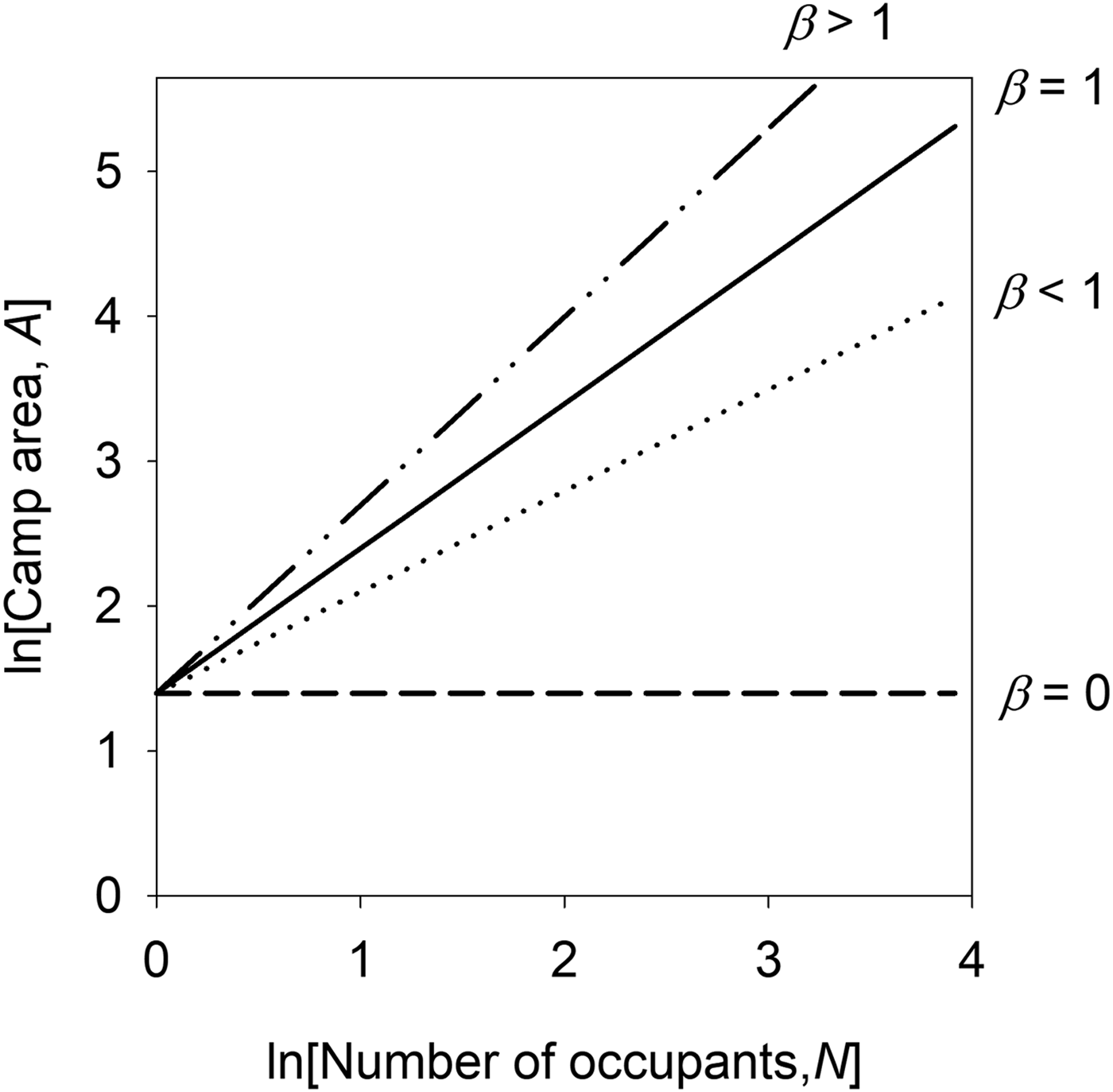
In this article, we are interested in how camp size and structure vary over time and space. Consider a simple case where N individuals occupy a camp of size A m2 after a residence of t days. So, A = f(N,t). For a given residency time, we can ask how camp areas vary with different numbers of occupants (see Figure 1). There is no a priori theoretical reason this change must be linear, or additive, though it may be. So, we require a model that allows but does not assume linearity. Thus, the appropriate model of these dynamics is lnA(N) = lnc + βlnN, or, on the linear scale, A(N) = cN β. If β = 1, then there is a simple linear increase of area with each occupant. If β < 1, then camp areas increase at a slower rate than the number of occupants, and so camps become increasingly dense the more occupants there are. If β = 0, then camp area is invariant to the number of occupants and remains a constant size regardless of the number of occupants. If β > 1, then relative camp area increases faster than the relative number of occupants, and so camp areas become increasingly diffuse with the number of occupants. In this article, we consider this scenario exactly, in addition to asking how camp area increases with residency time. We also ask how the number of features varies as a function of both the number of occupants and the residency time. The relative size (and sign) of the scaling exponent β provides a quantitative description of these dynamics.
Hypothetical example of scaling analysis, where power functions become linear functions on log-log axes and the various possible values of the scaling exponent, β, quantify the potential range of dynamics between camp area, A, and the number of occupants, N (assuming β ≥ 0).

Materials and Methods
The Data
Data were included based on two main criteria: (1) direct ethnoarchaeological observation of hunter-gatherer camps that included either a count of physical household features, or the spatial extent of camps, or, as in most cases, both; and (2) that the published (or recorded) study included at least two continuous variables of the four we were interested in for our study (see below for definitions). It was not possible to make our selection criteria stricter, as few ethnoarchaeological studies of hunter-gatherer camps report all four continuous variables.
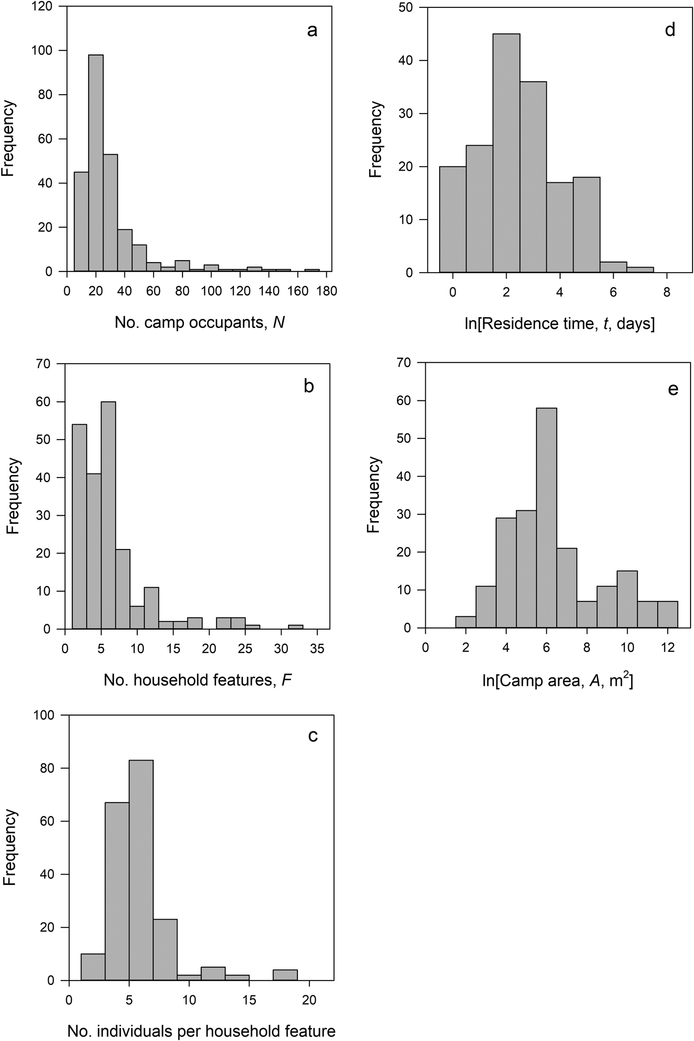
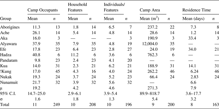
Our data include 11 hunter-gatherer populations, compiled from 13 published studies (as well as our own data), that met our inclusion criteria. These studies provided 263 ethnoarchaeological observations of hunter-gatherer camps, including groups from the Arctic, Australia, Africa, and South America (Supplemental Table 1). For each campsite observation, where possible, we collected data on (1) number of camp occupants, (2) number of household features (hearths, windbreaks, etc.), (3) camp area in square meters, (4) residence time in days, and (5) general environment (arid, forest, Arctic). Not all variables were available for all camps; therefore sample sizes vary with tests and are reported in the “Results” section. Table 1 and Figures 2 and 3 provide data summaries.
Frequency distributions of the ethnoarchaeological data used in this article by the primary variables under investigation: (a) number of camp occupants (n = 249); (b) number of household features (n = 208); (c) number of individuals per household feature (n = 196); (d) occupational residence times for camps (n = 163); (e) camp area, in square meters (n = 200).

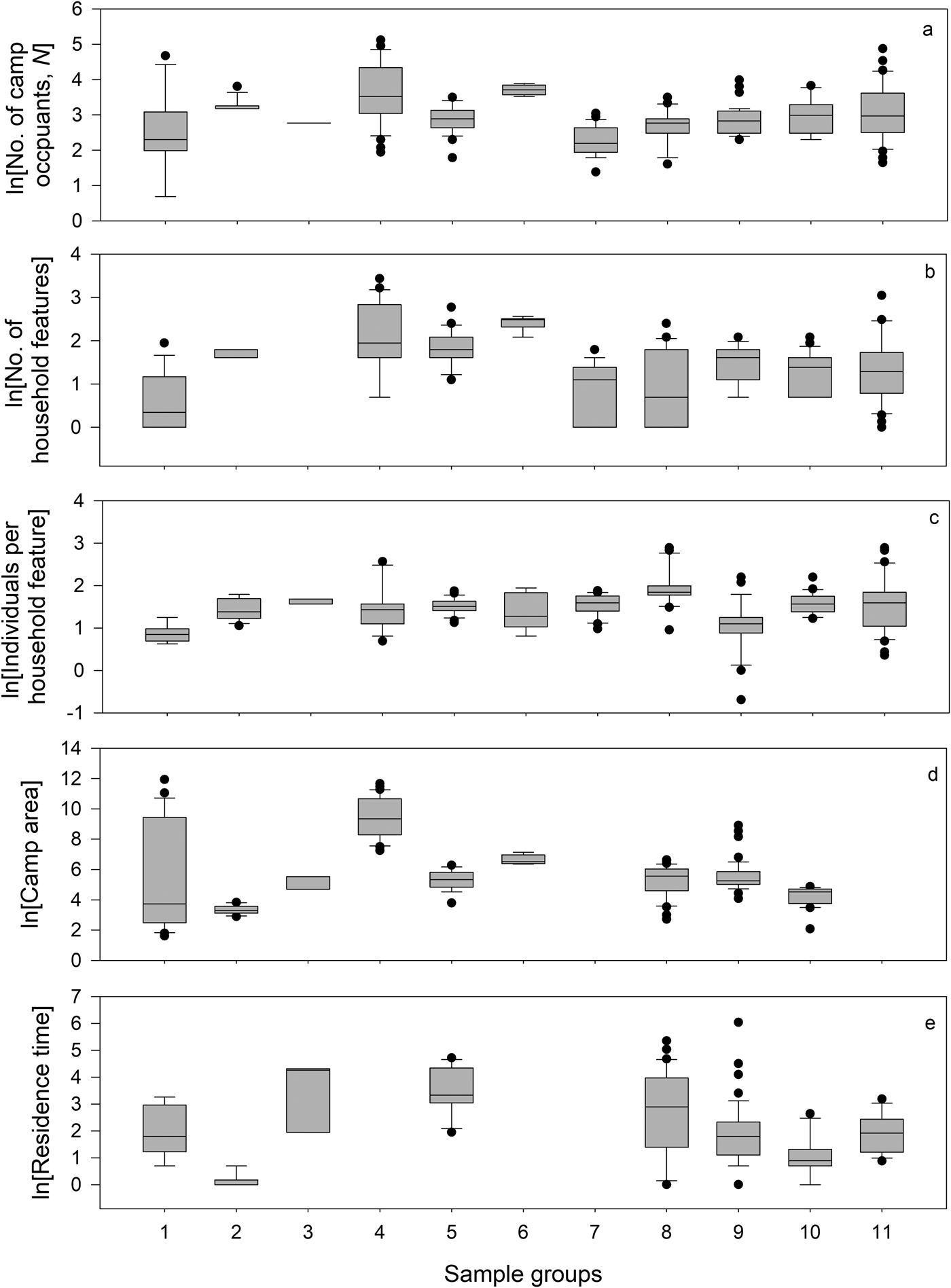
Box plots by study group: (a) number of camp occupants; (b) number of household features; (c) number of individuals per household feature; (d) camp area; (e) residence time. 1 = Western Aborigines; 2 = Ache; 3 = Aka; 4 = Alyawara; 5 = Efe; 6 = Hadza; 7 = Hill Pandaram; 8 = Kua; 9 = Dobe !Kung; 10 = Nukak; 11 = Nunamiut. (For sample sizes, see data in Supplemental Table 1.)

Summary Statistics for Ethnographic Groups.

Note: Means are geometric means—the exponentiated means of the logged data. C.I. = confidence interval.
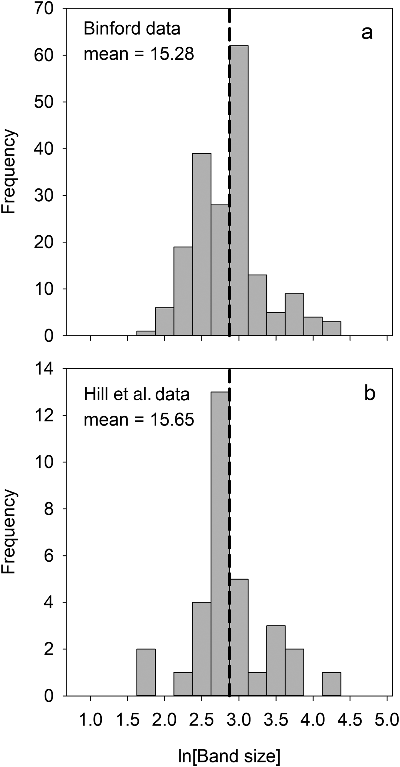
For our first set of analyses we compared our ethnoarchaeological data with compilations of ethnographic data (Figure 4a). The ethnographic data are primarily from Binford (Reference Binford2001) but also from Hill and associates (Reference Hill, Walker, Božičević, Eder, Headland, Hewlett, Hurtado, Marlowe, Wiessner and Wood2011; see Supplemental Tables 2 and 3). All data were restricted to residentially mobile hunter-gatherer populations, where entire groups move from camp to camp (variable GRPAT 1 in Binford Reference Binford2001), as opposed to semisedentary groups that operate out of a central location and form logistic camps only. Variables include (1) family size (Binford [2001:Table 8.1] estimated average family size for each group from the number of married males in a group) and (2) group size (i.e., band size; Binford's [2001:Table 8.1] variable Group 1), which is defined as an estimate of the average group size during the most dispersed part of the year. Data on the number of bands and the total number of people in those bands for 32 ethnographically recorded hunter-gatherer groups were also taken from Hill and associates (Reference Hill, Walker, Božičević, Eder, Headland, Hewlett, Hurtado, Marlowe, Wiessner and Wood2011; Figure 4b).
Frequency distributions of hunter-gatherer band sizes from (a) Binford Reference Binford2001 (n = 189) and (b) Hill et al. Reference Hill, Walker, Božičević, Eder, Headland, Hewlett, Hurtado, Marlowe, Wiessner and Wood2011 (n = 32).

These two estimates allowed us to calculate average band size per group by dividing the total number of people by the number of bands. Hill and associates (Reference Hill, Walker, Božičević, Eder, Headland, Hewlett, Hurtado, Marlowe, Wiessner and Wood2011) use the experienced band size, which provides a statistical estimate of the size of the band experienced by a random individual in the sample (see Greisser et al. Reference Greisser, Ma, Webber, Bowgen and Sumpter2011). Because the distributions of the sizes of bands are skewed, experienced band sizes are larger than the average band size. However, in this study, we use the average band size, as the quantity of interest to us is not the average size of a band experienced by a random individual in the sample but the average size of a hunter-gatherer band when it was observed ethnographically.
Data Treatment and Statistical Analyses
All continuous data were skewed on the arithmetic scale and so were normalized by log-transformation prior to analysis. The first stages of the analysis used t-tests, analyses of variance (ANOVAs), Mann-Whitney tests, and Kruskal-Wallis tests. To conduct the scaling analyses, it was necessary to control for random and fixed effects using mixed linear models (MLMs), which were run in Minitab 18. Our MLMs are fit using restricted maximum likelihood methods and so do not produce traditional measures of goodness of fit, such as r 2 and p-values. However, the statistical output includes pseudo-r 2 estimates, with associated p-values.
Results
Ethnoarchaeological Camp Variables by Sample Groups
Figure 3a–e shows five box plots of ethnoarchaeological hunter-gatherer camp data by sample group. A series of one-way ANOVAs and Kruskal-Wallis tests (Supplemental Table 4) show that average values vary significantly by sample group. As such, we control for group identity in our analyses (i.e., sample averages and sample group as a random effect in the MLMs).
The Scale of Hunter-Gatherer Camp Sizes
Average Number of Camp Occupants
The number of camp occupants in our dataset ranged from 2 to 167 across 249 camps. The frequency distribution of these data is lognormal (Figure 2a), and the geometric mean is 19.2 (14.7–25.0 occupants using a 95% confidence interval [C.I.]; Table 1).
Average Number of Camp Occupants by Habitat
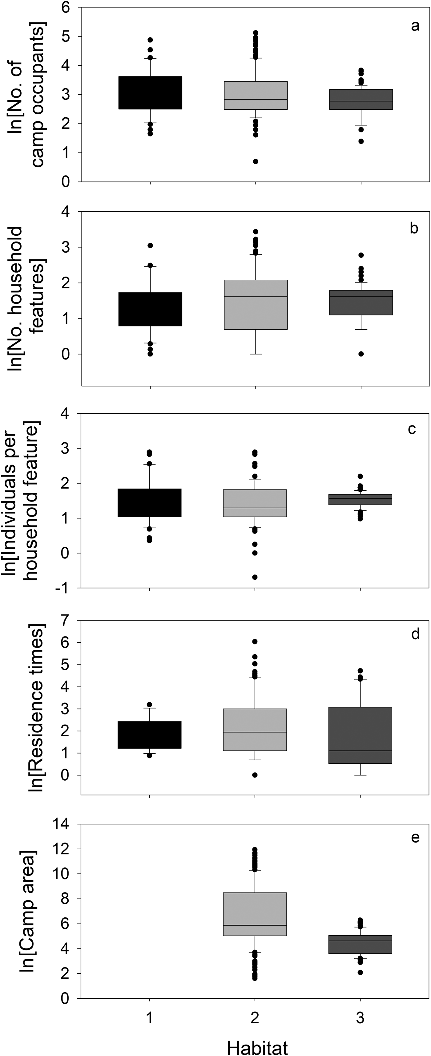
An ANOVA on the logged data of the number of camp occupants across habitats shows no significant difference at the p = 0.05 significance level (df = 2, 248, F = 2.73, p = 0.07; Figure 5a). A Kruskal-Wallis test on the linear data across the three habitat types also showed no significant difference (df = 2, H = 2.80, p = 0.23).
(a–e) Box plots of camp variables by habitat type: 1 = Arctic; 2 = arid; 3 = forest. Analysis of variance results are given in Supplemental Table 4 (for sample sizes, see data in Supplemental Table 1).

Number of Camp Occupants and Average Band Sizes
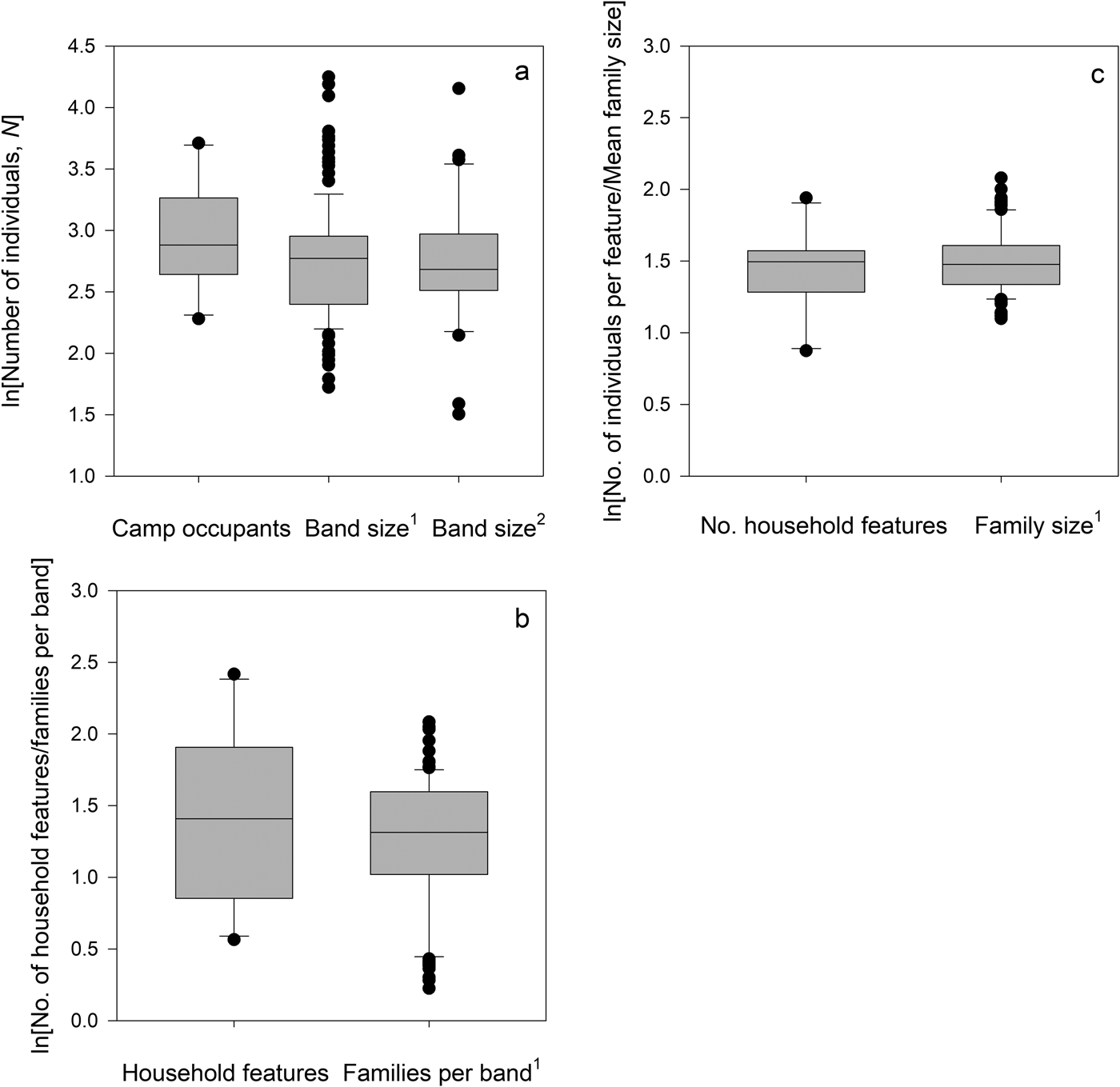
As above, the average number of occupants per camp was 19.2 (14.7–25.0 occupants using a 95% C.I.). The average size of bands in Binford's data is 15.28 (95% C.I.: 14.29–16.34), and the average size of bands in Hill and colleagues’ data is 15.65 (95% C.I.: 14.44–16.86). Controlling for group identity in the ethnoarchaeological sample, a one-way ANOVA across the three datasets shows no significant difference in estimates of average group size (df = 2 and 473; F = 1.13; p = 0.29; Figure 6a).
Box plots: (a) individuals per camp (n = 11) compared with bands (Binford Reference Binford2001; n = 189) versus band size (Hill et al. Reference Hill, Walker, Božičević, Eder, Headland, Hewlett, Hurtado, Marlowe, Wiessner and Wood2011; n = 32); (b) number of household features (n = 10) compared with families per group (n = 97); (c) individuals per feature (average per ethnographic group, n = 10) compared with average family size (n = 115). 1 = average band size data from Binford Reference Binford2001; 2 = average band size data from Hill et al. Reference Hill, Walker, Božičević, Eder, Headland, Hewlett, Hurtado, Marlowe, Wiessner and Wood2011.

Average Number of Features per Camp
The number of features in our dataset ranged from 1 to 31 across 207 camps. The frequency distribution of these data is lognormal (Figure 2b), and the geometric mean is 4.2 features per camp (95% C.I.: 2.9–6.1; Table 1).
Average Number of Household Features per Camp by Habitat
An ANOVA on the logged data of the number of features per camp across habitats shows no significant difference (F [3,207] = 0.29, p = 0.75; Figure 5b). We also conducted a Kruskal-Wallis test on the linear data across the three habitat types that similarly showed no significant difference (df = 2, H = 2.18, p = 0.53).
Average Number of Household Features per Camp and Average Number of Families per Band
The average number of household features per camp was 4.21 (95% C.I.: 2.93–6.07), and the average number of families per band in the ethnographic sample was 3.34 (95% C.I.: 3.03–3.70). Controlling for group identity by taking the average within each group, a paired t-test on the logged data shows that there is no significant difference between the number of families per group in the ethnographic sample and the number of features per camp (t-test: df = 10, p = 0.82; Figure 6b).
Average Number of Individuals per Household Feature
The average number of individuals per household feature in our dataset ranged from 0.5 to 18 (95% C.I.), across 196 camps. The frequency distribution is lognormal (Figure 2c), and the geometric mean is 4.6 individuals per feature (95% C.I.: 3.9–5.4; Table 1).
Number of Individuals per Household Feature by Habitat
An ANOVA on the logged data of the number of features per camp across habitats shows no significant difference (F [2, 195] = 2.07, p = 0.13; Figure 5c). We also conducted a Kruskal-Wallis test on the linear data across the three habitat types that similarly showed no significant difference (df = 2, H = 4.61, p = 0.10).
Number of Individuals per Household Feature and Average Family Size
The average number of individuals per feature per camp was 4.62 (95% C.I.: 3.94–5.42), and the average family size in the ethnographic sample is 4.50 (95% C.I.: 4.28–4.73). Controlling for group identity by taking the average within each group, a paired t-test on the logged data shows that there is no significant difference between the number of families per group in the ethnographic sample and the number of features per camp (df = 10, p = 0.75; Figure 6c).
Average residence time, habitat, and camp area
Additional tests of our data showed that the average residence time (Figure 2d) across our sample was 7.9 days (95% C.I.: 3.6–17.7; Table 1), and an ANOVA showed no significant difference in the average residence time across habitats (F [2, 162] = 1.11, p = 0.33; Figure 5d). Of the variables we considered, habitat only had a significant effect on camp area (Figure 5e; Table 1), where camps in arid habitats are significantly larger than camps in forest habitats (an average of 652 m2 as opposed to 82 m2; arid hunter-gatherer camps are about eight times the size of forest camps). Unfortunately, we have no estimates for Arctic camp size area in our sample.
The Dynamics of Hunter-Gatherer Camp Sizes
Given that we have established the average properties of hunter-gatherer camps and have shown that they accurately reflect the social structure of hunter-gatherer bands, we now consider the dynamics that cause variation in individual camp sizes using scaling analysis. We use mixed linear models where group identity, G, is a random effect and habitat type, H, is a fixed effect.
Number of Household Features by Number of Camp Occupants
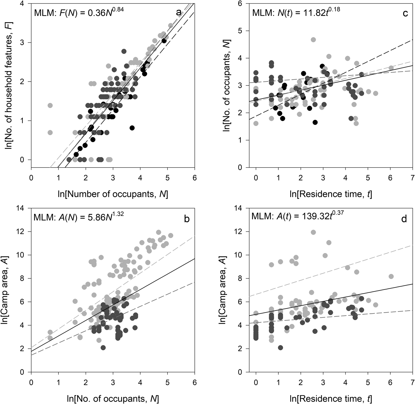
Figure 7a shows that the number of household features increases sublinearly. The scaling parameter estimate from the MLM is α = 0.84 (Supplemental Text 1), demonstrating that camps with more occupants have more household features but fewer than a simple linear expectation. Indeed, the scaling exponent describes an 84% increase in the number of features relative to the number of camp occupants, meaning that larger camps have a tendency to have more people on average using a feature. Figure 7a also shows the MLM results by color-coded habitat. The MLM results indicate that neither habitat nor the interaction of habitat by occupants is significant. As such, the number of household features increases at the same rate with the number of occupants across habitats.
Bivariate scaling plots: (a) number of household features by number of occupants (n = 196 total data points); (b) camp areas by number of occupants (n = 188); (c) number of occupants by residence times (n = 161); (d) camp areas by residence times (n = 141). Black lines are mixed linear model (MLM) fits to all data, Dashed lines are fits by habitat type: black = Arctic; light gray = arid; dark gray = forest.

Camp Area by Number of Camp Occupants
Figure 7b shows the increase in camp area as a function of the number of occupants. The MLM estimates that area increases as A : N 1.32 (Supplemental Text 1). As such, camp area increases by ~130% relative to the number of camp occupants. Therefore, camp densities (N / A) are not constant, and larger camps are more diffuse than smaller camps. Figure 7b also shows the data by habitat. The MLM results show that neither the effects of habitat nor the effects of group identity are significant, nor are their interaction terms. Therefore, while the area used per individual is approximately the same between the two habitat types (arid and forest), the area of arid camps increases with the number of occupants approximately as A : N 1.6, whereas in forests, camp area increases with occupants as A : N 1 (though the difference between the slopes is nonsignificant). As such, we hypothesize that in arid habitats, where camp size is less likely to be physically constrained by biomass, such as trees, there is a repulsive force between individuals, and so camps become increasingly diffuse with increasing numbers of occupants. At the other extreme, in forest camps, where camp size is likely to be more physically constrained by biomass, the area of a camp increases linearly with the number of occupants, and so camp density remains constant. Unfortunately, we have no data on the areas of Arctic camps.
Number of Camp Occupants by Residence Time
Figure 7c shows the number of occupants by residence time. The MLM shows a positive and significant relationship, with the number of occupants increasing with residence time as N : t 0.18 (Supplemental Text 1). However, as the slope is relatively shallow, only camps that are used for considerable lengths of time will be occupied by significantly larger numbers of individuals. When the data are separated by habitat type (Figure 7c), camps in forests show no trend between the number of occupants and residence time. In arid habitats, the number of occupants and residence time increase as N : t 0.2, and in the Arctic there is a steeper positive response, where the number of occupants increases at longer-term camps at a rate of N : t 0.4, though the difference between these slopes is marginally nonsignificant at the 0.05 significance level (p = 0.053).
Camp Area by Residence Time
Figure 7d shows camp area as a function of residence time. The MLM results indicate that camp area increases with residence time at a rate of about A : t 0.37 (for details, see Supplemental Text 1). As such, camps occupied for longer are larger, but the rate of increase is less than linear. If camp area increased linearly with time (i.e., A : t), this would suggest that camp occupants effectively perform random walks (i.e., simple diffusion) from a starting location (i.e., the center of the camp). However, as the observed slope is much shallower, this suggests a tethered diffusion process, where occupants (and their debris) are increasingly distributed in space through time, but this tendency to spread is tethered to a central location, such as a household feature. By habitat, the results show that there is a significant habitat effect (i.e., camps are significantly larger in arid regions than in forest regions; p = 0.001), and the interaction between habitat type and time is also significant (p = 0.001), where the rate of increase of camp area over time is faster in arid habitats (A ~ t 0.6) than in forests (A ~ t 0.15).
Camp Area by Number of Occupants and Residence Time
We combine the effects of the number of occupants and residence time on camp areas in a single model (including a significant interaction term between habitat and occupants) of the form y(x 1, x 2/G, H) = cx 1β1× 2β2(x 1× 2)β3. We find that both the number of occupants and residence time are significant predictors of camp area, with an overall model fit of pseudo-r 2 = 0.91 (Supplemental Text 1). Camp areas in forests increase as A Forest(N,t) = 3.31N 1.03t 0.11 and in deserts increase as A Arid(N,t) = 38.09N 0.80t 0.48, where the normalization constants have units of area (m2) per individual per day. As such, this model shows that the effects of the number of occupants on camp area are similar across habitats, and the primary difference in camp areas between the two habitats is the effect of residence time, where camp size increases in area in response to increasing residence time much faster in deserts than in forests.
Discussion
Scale
The results from the first stage of our analyses show that there are commonly about four infrastructural features, such as hearths or windbreaks, on average in a hunter-gatherer camp. Moreover, this average does not vary across different environments. This result is consistent with ethnographic data that show that, on average, hunter-gatherer bands are composed of about four families and that this size holds across environments (Hamilton, Milne, Walker, and Brown Reference Hamilton, Milne, Walker and Brown2007). Moreover, in all three datasets used in this article, average hunter-gatherer band sizes are consistently smaller than 25 individuals. We derive the average number of individuals per feature by dividing the number of camp occupants by the number of features and find that there are 4.6 individuals per feature. This number is consistent with average family size data from ethnographic observations. The first stage of our analyses thus shows that the internal infrastructural organization of hunter-gatherer camps is consistent with independent measures of the social organization of hunter-gatherer bands. The fact that the distribution of the number of occupants per individual camp in our dataset is consistent with the distribution of average band sizes across hunter-gatherer societies is both a consistency check between the datasets and further evidence of the universal size and modularity of hunter-gatherer social organization, reflected both in the internal social structure of bands and in the archaeological signature of their camps.
Let us assume that the sample of ethnoarchaeological observations of hunter-gatherer camps is reflective of the population of prehistoric hunter-gatherer camps. This is the same as assuming that the set of physical, biological, economic, and cultural factors that constrain the scale of hunter-gatherer camps and bands in the ethnohistoric record operated similarly in the past (Kelly Reference Kelly2013). Given the robust nature of the average hunter-gatherer band size, from a number of independent datasets (i.e., Binford Reference Binford2001, Hill et al. Reference Hill, Walker, Božičević, Eder, Headland, Hewlett, Hurtado, Marlowe, Wiessner and Wood2011, and ours), this is at least a plausible assumption. Or to state this assumption alternatively, there is no a priori reason to assume that the constraints that set the scale of hunter-gatherer social organization in the past differed significantly from those operating in the ethnohistoric present such that the universality of hunter-gatherer band sizes we see across datasets is an irrelevant baseline in understanding prehistoric hunter-gatherer social structure and behaviors. Accepting this, because our results show a direct link between the sizes of hunter-gatherer bands and the physical features of the camps they form, our findings have several interesting implications for understanding the scale of hunter-gatherer campsites in the archaeological record.
Our results suggest that hunter-gatherer camping locales commonly consist of several hearth/residential features, occupied by multiple coresident families. Table 1 indicates that the average number of coresiding families in a camp is about four (or between three and six at a 95% C.I.), and this number does not change significantly across different habitats. Moreover, the lognormal probability distribution of the number of household features in a camp is highly peaked around the mode (Figure 2b), and so the probability of observing a camp with more than the average number of features decreases exponentially. Not only does this imply a well-defined expectation for the number of coresiding families at prehistoric hunter-gatherer camps, but it suggests that if large hunter-gatherer camps are identified in the archaeological record, they likely represent aggregations of multiple bands, and thus we can infer that these are rare occurrences based on the ethnographic data. Whether large sites with multiple features are reoccupations made by individual bands over time or single large-scale aggregation events is, of course, a question that can only be answered on a site-by-site basis (see Binford Reference Binford1982; Haas et al. Reference Haas, Klink, Maggard and Aldenderfer2015; Hamilton et al. Reference Hamilton, Buchanan, Huckell, Holliday, Shackley and Hill2013; LaBelle Reference LaBelle, Hurst and Hofman2010; Surovell Reference Surovell2009). Therefore, the archaeological signature of hunter-gatherer camps is likely to be the inverse of the actual ethnographic occurrence, as larger camps will leave a much greater archaeological signature than smaller camps, while being rarer events. It is important to note that the largest reported camp areas in our sample are arid Australian camps at ~12,000 m2, whereas the largest forest camps are Efe camps, ~530 m2, approximately a 20-fold difference. Most archaeological excavations will only be able to sample a small proportion of the actual camp area, and thus there will be a tendency to underestimate the extent of an occupation. For scale, a 12,000 m2 camp is an occupation area of more than 110 × 110 m or a circular occupation area with a diameter of ~125 m. Of course, this assumes that individual occupations belonging to the same camping event can be identified archaeologically.
While hunter-gatherer band sizes and structures are statistically similar across habitat types, they vary significantly across individual groups in our sample (Figure 3; Supplemental Table 4). This result suggests that within any particular habitat individual bands may vary in size and composition but that this variance is constrained such that average sizes across habitats are statistically consistent. The size of any hunter-gatherer band at a particular point in time and space will be both demographically and historically contingent. Band sizes vary due to variation in local environmental conditions and circumstances and recent historical events that temporarily impact population numbers (e.g., warfare, disease, natural catastrophes, environmental booms or busts), as well as to stochastic demographic processes in small-scale populations (Hamilton and Walker Reference Hamilton and Walker2018). For example, the average number of camp occupants in our ethnoarchaeological data ranges from 11.3 among Western Aborigine groups to 40.8 among the Hadza, an approximately fourfold difference. However, the differences in average camp sizes across groups within similar environments are statistically nonsignificant. In Binford's data, the only groups with band sizes larger than 40 individuals are ethnohistoric North American equestrian societies, such as the Comanche, Crow, and Blackfoot, who due to their use of the horse, among other historically contingent circumstances, would have experienced very different ecological, economic, and energetic constraints to the size of their bands than pedestrian foraging societies.
While the evolutionary ecology and economics of hunter-gatherer family formation are well studied (e.g., Hooper et al. Reference Hooper, Winking, Gurven and Kaplan2015; Kaplan et al. Reference Kaplan, Hooper and Gurven2009; Lancaster and Kaplan Reference Lancaster, Kaplan, Nishida, McGrew, Marler, Pickford and Van de Waal1992), the dynamics of hunter-gatherer group size are much less so and remain a central question in hunter-gatherer studies. Because hunter-gatherer group size does not vary predictably with environmental variability, group size must be related to general constraints on the size of social networks humans require to effectively forage for heterogeneously distributed resources while maintaining social ties with both kin and non-kin in low-density, mobile populations. As such, this suggests that variations in hunter-gatherer group size, ultimately, are more evolutionary than ecological. Boone (Reference Boone, Smith and Winterhalder1991) outlines various economic models that lay out the conditions under which an optimal group size may evolve, given the nonlinear trade-offs to increasing individual foraging returns by increasing group membership. However, while these models provide potential economic mechanisms for group size optimization, the observed robustness of hunter-gatherer group sizes across different environments suggests that these economic trade-offs must also be ecologically invariant.
Our results suggest some important implications for understanding the scale of hunter-gatherer band size. On average, at or near demographic equilibrium, a hunter-gatherer band will be composed of about 20 individuals, half male and half female, about half of whom will be adults and half of whom will be unmarried offspring (in nonequilibrium growth phases, average family size will be larger than the demographic replacement of two adults and two offspring, and so bands will be composed of less than half adults and more than half offspring). If we accept that hunter-gatherer nuclear families form due to the time and energy costs to mothers raising dependent offspring, and the subsequent need for fathers’ investment of energy to mother and offspring through hunting, then there must be something about the economic calculus of coresiding in bands of multiple families that facilitates offspring survival and stabilizes long-term foraging return rates (see Kelly Reference Kelly2013). As daily hunting success rates are highly variable, and reciprocal exchange partnerships between hunters evolved to ameliorate this inherent variability (i.e., Gurven Reference Gurven2004; Hill and Kintigh Reference Hill and Kintigh2009), our results suggest that the variability in daily hunting success can be compensated effectively by ~five male hunters (excluding the possibility that subadult males contribute significantly to the group energy budget; see Gurven et al. Reference Gurven, Kaplan and Gutierrez2006; Walker et al. Reference Walker, Hill, Kaplan and MacMillan2002; Winterhalder Reference Winterhalder1986). Moreover, significantly more than this number of adult male hunters must quickly lead to decreasing per capita returns in any environment, despite the fact that additional hunters will only continue to decrease individual variation in hunting success (i.e., the law of large numbers). However, why the dynamics of hunter-gatherer band formation converge to an equilibrium of about 20 individuals (not 50, 100, or 1,000, for example) has yet to find a theoretically satisfying explanation.
Dynamics
Our scaling results show that the dynamics governing the variation of hunter-gatherer camp size and structure are also largely consistent across habitats. The number of household features in a hunter-gatherer camp increases less than proportionally with the number of camp occupants (Figure 7a). This sublinear scaling quantifies an economy of scale in camp infrastructure with camp size, such that larger camps require proportionally fewer features to support more individuals. In fact, this sublinear scaling is a common feature of infrastructure–population size scaling in all types of human societies, from hunter-gatherers and subsistence agriculturalists to contemporary cities and nation-states (Bettencourt et al. Reference Bettencourt, Lobo, Helbing, Kühnert and West2007; Freeman Reference Freeman2016; Hamilton, Milne, Walker, and Brown Reference Hamilton, Milne, Walker and Brown2007; Ortman and Coffey Reference Ortman and Coffey2017; Ortman et al. Reference Ortman, Cabaniss, Sturm and Bettencourt2014, Reference Ortman, Cabaniss, Sturm and Bettencourt2015; Ortman et al. Reference Ortman, Davis, Lobo, Smith, Bettencourt and Trumbo2016). However, in small-scale camps this economy of scale would only be observable in the largest camps. As this increase is due to neither increases in average family size nor increases in the number of families per camp, it may be because larger camps attract proportionally more visitors. Mechanisms that may account for this include preferential attachment, where the number of migrants at a location increases proportionally with the size of that location, a dynamic underlying the statistics of urban growth in industrialized societies. But importantly, our MLM shows that this dynamic is consistent across Arctic, arid, and forest habitats. Therefore, not only is the scale or average number of occupants at camps consistent across habitats, but so are the dynamics governing their variance.
Similarly, both variation in the number of occupants and camp areas as a function of residence time are largely consistent across habitats. Figure 7c shows that when controlling for either sample group or habitat type, there is a shallow positive increase between the number of camp occupants and the length of residence time. However, the statistical summaries in Supplemental Text 1 show no significant relationship between camp size and residence time across habitats, though on average Arctic camps have more occupants than those in other habitats. This pattern suggests that while camp residence times may vary across habitats, the size of bands is constant in arid and forest habitats. In the Arctic, camps tend to be occupied by larger groups, suggesting that larger camps may attract an increasing number of visitors, as discussed above.
Figure 7b, d, summarizes the response of camp area to variation in the number of camp occupants and residence time (we have no spatial camp size data for Arctic cases, and so we only report results for arid and forest habitats). Camp area responds differently to an increase in the number of occupants in arid and forest environments. In arid environments, camp area increases rapidly with the number of camp occupants at a superlinear rate, A Arid ~ N 1.6. This rate is much faster than a proportional response (A ~ N 1), where each additional occupant adds a constant area to the total camp area. This implies that there is a repulsive force, or a tendency of individuals (or households) to separate themselves in space from each other in increasingly larger camps. This may be because in arid, open environments, the spatial extent of camp boundaries is less constrained by the physical environment, and so each household can easily maintain contact with the others while maximizing its individual space. Another reason may be that if there were decreased rates of sharing among family groups in larger camps, individual families might have a tendency to camp farther apart from each other. Camp occupant density thus decreases as N / A Arid ~ N −0.6 in arid environments, and so arid environments’ larger camps become increasingly diffuse on the landscape. In forests, we see a very different relationship between area and individuals. Camp areas increase linearly with the number of occupants, A Forest ~ N 1. Therefore, each additional individual in forest camps increases total camp size by a constant amount. Camp occupant density in forests is thus invariant to the number of occupants, N / A Forest : N 0.
In both arid and forest habitats, camp areas increase with residence time at the same rate, A ~ t 0.37 (Figure 7d; Supplemental Text 1). This result indicates that camp areas tend to increase with residence time in both habitats, but at a less-than-proportional rate, as would be expected from a simple random walk model, A : t 1. As such, camp areas increase in size because camp debris is increasingly deposited in space around activity areas, but activities are centered around household features, resulting in a tethered diffusion process rather than a purely diffusive process. However, when we model camp area as a function of both camp occupants and residence time in a mixed model, we find that in both environments the effect of increasing camp occupants is nearly linear on camp size, but the difference is in residence time. So, this suggests that the addition of new individuals to a camp increases total camp area by a constant rate, but the tendency of the spatial extent of a camp to increase over time is greater in arid than forest environments.
While understanding these dynamics is important for considering hunter-gatherer camps in the archaeological record, the implications are not simple. Complicating the archaeological interpretation of camp area, the results of the combined mixed model (see Supplemental Text 1) show that camp areas increase as a function of both the number of occupants and residence times. This means that large-scale camps could have been occupied either by a large number of residents, or for an extended period of time, or both. Analysis of the ethnoarchaeological record does not allow us to parse the two alternatives. An archaeological estimate of the number of household features, such as hearths, may be closely correlated with the number of occupants (Figure 7a), but the number of features in itself contains no information about residence time (Figure 7c). Therefore, estimates of the residence time of a camp will have to come from other lines of archaeological evidence, such as the density, scale, and spatial distribution of occupational debris around features (see Binford Reference Binford1982, Reference Binford1983; Yellen Reference Yellen1977). The best estimates of residence times will be relative measures that require the excavation of multiple residential features and multiple camps of comparative age and environmental setting.
We have shown that both the scale and the dynamics governing variation in hunter-gatherer camps hold across different environments. Moreover, we have shown that the internal physical structure of hunter-gatherer camps manifest in infrastructural features, such as hearths or windbreaks, is consistent with the known ethnographic social organization of hunter-gatherer bands. The universal size and structure of hunter-gatherer bands can be observed both in the ethnographic record and in the physical infrastructure of their camps.
Acknowledgments
We thank Robert Kelly and three anonymous reviewers for their comments. We also thank Michael Whalen for translating the abstract into Spanish.
Data Availability Statement
All data used in this article are available in Supplemental Tables 1, 2, and 3.
Supplemental Materials
For supplementary material accompanying this article, visit https://doi.org/10.1017/aaq.2018.39.
Supplemental Text 1. Summary of Results of Mixed Linear Models
Supplemental Table 1. Ethnoarchaeological Hunter-Gatherer Data Used in Analyses.
Supplemental Table 2. Comparative Hunter-Gatherer Data from Binford Reference Binford2001 Used in Analyses.
Supplemental Table 3. Comparative Hunter-Gatherer Data from Hill et al. Reference Hill, Walker, Božičević, Eder, Headland, Hewlett, Hurtado, Marlowe, Wiessner and Wood2011 Used in Analyses.
Supplemental Table 4. Summary of Analyses of Variance and Kruskal-Wallis Tests across Sample Groups.