

1. Introduction
The prevalence of shear in fluids makes it one of the most common sources of turbulence in nature. As such, interest in the linear and nonlinear stability of shear flows dates as far back as the 19th century to the early works of Reynolds (Reference Reynolds1883) and von Helmholtz (Reference von Helmholtz1896), and still continues today. A large class of shear-driven instabilities can loosely be categorized as Kelvin–Helmholtz (KH) instabilities, which occur in plane-parallel continuous or interfacial shear flows (Chandrasekhar Reference Chandrasekhar1961; Drazin & Reid Reference Drazin and Reid1981). Turbulence driven by KH instabilities can cause substantial mixing of momentum, heat and/or chemicals in fluid bodies such as the Earth's atmosphere, oceans and liquid core, as well as planetary and stellar atmospheres and interiors. Quantifying shear-induced mixing is therefore a crucial step towards improving evolutionary models of these large-scale systems.
In fluids that are composed of partially or fully ionized plasma (e.g. stellar interiors, magnetically confined laboratory plasmas, etc.), or made of liquid metals (e.g. planetary interiors), magnetic fields and the forces they exert must also be taken into account. Studies of the stability and mixing properties of parallel shear flows in that context are often performed using the magnetohydrodynamic (MHD) approximation (see, e.g. Chandrasekhar Reference Chandrasekhar1961; Hughes & Tobias Reference Hughes and Tobias2001), with a few notable exceptions (Rogers & Dorland Reference Rogers and Dorland2005; Henri et al. Reference Henri2013; Karimabadi et al. Reference Karimabadi2013; Faganello & Califano Reference Faganello and Califano2017; Fraser et al. Reference Fraser, Pueschel, Terry and Zweibel2018; Vogman et al. Reference Vogman, Hammer, Shumlak and Farmer2020).
Many of these MHD works additionally use the ideal limit, where both viscosity and resistivity are neglected (despite the fact that such mixing problems are often fundamentally ill-posed; see, e.g. Lecoanet et al. (Reference Lecoanet, McCourt, Quataert, Burns, Vasil, Oishi, Brown, Stone and O'Leary2016)). In ideal MHD, the magnetic field lines are frozen into the flow and are forced to move with it. Meanwhile, a magnetic tension proportional to the square of the field amplitude resists the deformation of field lines, and has a tendency to rigidify the flow, imbuing it with elastic-like properties. As a result, the presence of a magnetic field parallel to the mean flow can hinder the development of KH billows. It has been shown that, in the ideal limit, a uniform streamwise magnetic field stabilizes KH modes provided its Alfvén velocity exceeds the characteristic flow speed by a factor that depends on the flow profile but is typically of order unity (Chandrasekhar Reference Chandrasekhar1961).
Magnetic fields are also known to modify or fully invalidate several important exact theoretical results on the stability of incompressible, hydrodynamic, parallel shear flows. For example, Tatsuno & Dorland (Reference Tatsuno and Dorland2006) showed that magnetized shear instabilities can exist even when the background flow does not have an inflection point, contrary to the hydrodynamic case where the latter is necessary (Rayleigh Reference Rayleigh1879). Similarly, Lecoanet et al. (Reference Lecoanet, Zweibel, Townsend and Huang2010) provided examples of unstable magnetized stratified shear flows in which the Richardson number always exceeds  $1/4$, showing that the Miles–Howard theorem (Howard Reference Howard1961; Miles Reference Miles1961) does not apply in MHD. Finally, Hughes & Tobias (Reference Hughes and Tobias2001) showed that Howard's semicircle theorem (Howard Reference Howard1961) is modified in the presence of magnetic fields, and that the eigenvalues of the linear stability problem must now lie within the intersection of two semicircles in the complex plane, whose existence and position depend on the amplitude and profiles of the background flow and magnetic field.
In non-ideal MHD, the resistivity of the fluid allows the field to partially decouple from the flow, and reduces its (usually) stabilizing influence. For magnetized KH instabilities, gradually increasing the resistivity can thus raise the growth rate of unstable modes to a value between that obtained in the ideal MHD limit and in the hydrodynamic case (Palotti et al. Reference Palotti, Heitsch, Zweibel and Huang2008). It is also worth mentioning that by contrast with the hydrodynamic case, three-dimensional (3-D) perturbations are sometimes the fastest-growing modes in non-ideal MHD shear instabilities (Hunt Reference Hunt1966; Hughes & Tobias Reference Hughes and Tobias2001).
With these general results in mind, we investigate in this paper a very specific problem, namely the stability and evolution of a sinusoidal, incompressible shear flow with finite viscosity and resistivity, in the presence of a uniform, streamwise magnetic field. This problem is highly relevant to a number of applications but has not, to our knowledge, been studied in detail yet. Sinusoidal shear flows are defined here as unidirectional plane-parallel flows whose amplitude varies sinusoidally in the transverse direction. There is a relatively long history of studying sinusoidal shear flows in the hydrodynamic case, including both unstratified (Meshalkin & Sinai Reference Meshalkin and Sinai1961; Gotoh, Yamada & Mizushima Reference Gotoh, Yamada and Mizushima1983; Dubrulle & Frisch Reference Dubrulle and Frisch1991; Lucas & Kerswell Reference Lucas and Kerswell2014) and stratified (Balmforth & Young Reference Balmforth and Young2002) flows, in part because their periodicity means that they can be studied in the absence of physical boundaries, thus serving as a simple example of a shear flow whose evolution can be considered without the effects of boundary layers. They also commonly arise in nature from the development of a primary instability that results in the exponential growth of so-called ‘elevator’ modes, as in homogeneous Rayleigh–Bénard convection (Calzavarini et al. Reference Calzavarini, Doering, Gibbon, Lohse, Tanabe and Toschi2006; Garaud et al. Reference Garaud, Ogilvie, Miller and Stellmach2010), the double-diffusive fingering instability (Baines & Gill Reference Baines and Gill1969) and the Goldreich–Shubert–Fricke instability (Goldreich & Schubert Reference Goldreich and Schubert1967; Fricke Reference Fricke1968). In these examples, secondary shear instabilities between elevators flowing in opposite directions are thought to be responsible for the saturation of the primary instability and have successfully been used to model it in the hydrodynamic limit (Radko & Smith Reference Radko and Smith2012; Brown, Garaud & Stellmach Reference Brown, Garaud and Stellmach2013; Barker, Jones & Tobias Reference Barker, Jones and Tobias2019). These secondary instabilities are almost always studied in the so-called ‘frozen-in’ approximation (where the elevator mode velocity is assumed to be constant in time for the purpose of the linear stability analysis) and hence our interest in constant-amplitude sinusoidal flows in this work as well.
In the MHD case, the presence of a uniform magnetic field aligned with the direction of the primary elevator mode flow has no effect on its growth rate, but can stabilize the secondary shearing mode, for the reasons discussed earlier. As such, understanding the linear stability and nonlinear evolution of magnetized shear instabilities in sinusoidal shear flows is a key step in quantifying the effects of magnetic fields on homogeneous Rayleigh–Bénard convection, and on various double-diffusive instabilities (similarly, the stability of sinusoidal shear flows in MHD has been studied to understand the saturation of channel modes in the magnetorotational instability; see, e.g. Goodman & Xu (Reference Goodman and Xu1994), Latter, Lesaffre & Balbus (Reference Latter, Lesaffre and Balbus2009), Pessah & Goodman (Reference Pessah and Goodman2009), Longaretti & Lesur (Reference Longaretti and Lesur2010) and Pessah (Reference Pessah2010)). Finally, recent numerical simulations of double-diffusive fingering convection show that the effective kinetic and/or magnetic Reynolds numbers of the saturated nonlinear flow can remain modest over a broad range of parameter space (Brown et al. Reference Brown, Garaud and Stellmach2013). As such, diffusive effects (viscosity and resistivity) should be taken into account to correctly model the development of the secondary shear instabilities.
In this paper, we therefore investigate the linear stability and nonlinear saturation of a sinusoidal, incompressible shear flow in the presence of a uniform, streamwise magnetic field. We present the background state and linearized equations in § 2. Section 3 presents a linear stability analysis of this flow over a wide range of parameter space, demonstrating the presence of three distinct branches of instability, two of which have not, to our knowledge, been discussed before. We then focus on one of the two new branches, which exists even in the presence of very strong magnetic fields, and takes the form of overstable Alfvén waves. We derive a heavily truncated model for the unstable modes in § 4, and use it in § 4.2 to demonstrate that this instability is driven by the anti-diffusive properties of sinusoidal shear flows discussed by Dubrulle & Frisch (Reference Dubrulle and Frisch1991). In § 5 we present an illustrative example of the nonlinear evolution of this system using a direct numerical simulation, demonstrating a linear growth phase consistent with predictions from the linear stability analysis, and a saturated state dominated by counter-propagating solitons. We conclude in § 6 with a short discussion of the potential relevance of this new instability for natural systems, and of future work.
2. Model and linear stability analysis
We consider a background flow  ${\boldsymbol u}_E$ directed in the
 $z$ (streamwise) direction, whose amplitude varies sinusoidally in the
 $x$ (shearwise) direction. Units are selected based on the flow's amplitude
 $U^{*}$ and shearwise wavenumber
 $k_x^{*}$, and in these units
 ${\boldsymbol u}_E$ is given by
 \begin{equation} {\boldsymbol u}_E = \sin(x) {\boldsymbol e}_z \end{equation}
(the subscript ‘ $E$’ is used here to denote ‘elevator’, following the motivating example given in § 1). We assume that the background flow is maintained against viscous decay by an external force applied to the system, and is therefore a laminar steady-state solution of the governing equations (see below). We also assume the existence of a uniform background magnetic field
 $\boldsymbol {b}_E$ oriented in the streamwise direction, whose amplitude
 $B^{*}$ defines the unit magnetic field strength so that, in these units,
 \begin{equation} \boldsymbol{b}_E = \boldsymbol{e}_z. \end{equation}
The total flow and field are written as the sum of this background plus a perturbation, namely
 \begin{equation} {\boldsymbol u} = {\boldsymbol u}_E + \tilde{\boldsymbol u}, \quad {\boldsymbol b} = \boldsymbol{b}_E + \tilde{\boldsymbol b}, \end{equation}
and satisfy the governing equations
 \begin{equation} \left.\begin{array}{c@{}}
\displaystyle \dfrac{\partial {{\boldsymbol u}}}{\partial
t} + {{\boldsymbol u}} \boldsymbol{\cdot}
\boldsymbol{\nabla} {{\boldsymbol u}} ={-}
\boldsymbol{\nabla} p + C_B (\boldsymbol{\nabla} \times
{{\boldsymbol b}}) \times {{\boldsymbol b}} + \dfrac{1}{Re}
\nabla^{2} ({{\boldsymbol u}}-{{\boldsymbol u}}_E), \\
\displaystyle \dfrac{\partial {\boldsymbol b}}{\partial t}
= \boldsymbol{\nabla} \times ({\boldsymbol u} \times
{\boldsymbol b}) + \dfrac{1}{Rm} \nabla^{2} {\boldsymbol
b}, \\ \displaystyle \boldsymbol{\nabla} \boldsymbol{\cdot}
{{\boldsymbol u}} = 0 \quad \boldsymbol{\nabla}
\boldsymbol{\cdot} {{\boldsymbol b}} = 0.
\end{array}\right\} \end{equation}
Note the viscous term in the momentum equation, where the non-dimensional applied force has been written as  $-Re^{-1} \nabla ^{2} {\boldsymbol u}_E$. The non-dimensional parameters are the usual viscous and magnetic Reynolds numbers, as well as the ratio of characteristic magnetic and kinetic energies of the background flow (alternatively, an inverse Alfvénic Mach number squared), namely
 \begin{equation} Re = \frac{U^{*}}{\nu^{*} k_x^{*}}, \quad Rm = \frac{U^{*}}{\eta^{*} k_x^{*}} \quad \mbox{and}\quad C_B = \frac{(B^{*})^{2}}{\rho_0^{*} \mu_0^{*} (U^{*})^{2}}, \end{equation}
where  $\nu ^{*}$ and
 $\eta ^{*}$ are the (constant) kinematic viscosity and magnetic diffusivity of the fluid,
 $\rho _0^{*}$ is the constant density of the fluid and
 $\mu _0^{*}$ is the permeability of the vacuum. Note that the magnetic Prandtl number,
 $Pm = \nu ^{*}/\eta ^{*}$, is the ratio of
 $Rm$ and
 $Re$. It is usually smaller than one in stellar interiors, but not necessarily asymptotically small (Rincon Reference Rincon2019).
Linearization around the background state yields the evolution equations for the perturbations  $\tilde {{{\boldsymbol u}}}$ and
 $\tilde {{{\boldsymbol b}}}$ as
 \begin{equation} \left.\begin{array}{c@{}}
\displaystyle \dfrac{\partial \tilde{{{\boldsymbol
u}}}}{\partial t} + {{\boldsymbol u}}_E \boldsymbol{\cdot}
\boldsymbol{\nabla} \tilde{{{\boldsymbol u}}} +
\tilde{{{\boldsymbol u}}} \boldsymbol{\cdot}
\boldsymbol{\nabla} {{\boldsymbol u}}_E ={-}
\boldsymbol{\nabla} p + C_B (\boldsymbol{\nabla} \times
\tilde{{{\boldsymbol b}}}) \times {\boldsymbol e}_z +
\dfrac{1}{Re} \nabla^{2} \tilde{{{\boldsymbol u}}} , \\
\displaystyle \dfrac{\partial \tilde{\boldsymbol
b}}{\partial t} = \boldsymbol{\nabla} \times ({\boldsymbol
u}_E \times \tilde{\boldsymbol b})+ \boldsymbol{\nabla}
\times (\tilde{\boldsymbol u} \times {\boldsymbol e}_z) +
\dfrac{1}{Rm} \nabla^{2} \tilde{\boldsymbol b}, \\
\boldsymbol{\nabla} \boldsymbol{\cdot} \tilde{{{\boldsymbol
u}}} = 0 \quad \boldsymbol{\nabla} \boldsymbol{\cdot}
\tilde{{{\boldsymbol b}}} = 0 , \end{array}\right\}
\end{equation}
which can be expressed, component-wise, as
 \begin{equation} \left.\begin{array}{c@{}}
\displaystyle \dfrac{\partial \tilde{u}_x}{\partial t} +
\sin(x) \dfrac{\partial \tilde{u}_x}{\partial z} ={-}
\dfrac{\partial p}{\partial x} + C_B \left( \dfrac{\partial
\tilde{b}_x}{\partial z} -\dfrac{\partial
\tilde{b}_z}{\partial x} \right) + \dfrac{1}{Re} \nabla^{2}
\tilde{u}_x, \\ \displaystyle \dfrac{\partial
\tilde{u}_y}{\partial t} + \sin(x) \dfrac{\partial
\tilde{u}_y}{\partial z} ={-} \dfrac{\partial p}{\partial
y} - C_B \left( \dfrac{\partial \tilde{b}_z}{\partial y}
-\dfrac{\partial \tilde{b}_y}{\partial z} \right) +
\dfrac{1}{Re} \nabla^{2} \tilde{u}_y ,\\ \displaystyle
\dfrac{\partial \tilde{u}_z}{\partial t} + \sin(x)
\dfrac{\partial \tilde{u}_z}{\partial z} + \tilde{u}_x
\cos(x) ={-} \dfrac{\partial p}{\partial z} + \dfrac{1}{Re}
\nabla^{2} \tilde{u}_z, \\ \displaystyle \dfrac{\partial
\tilde{b}_x}{\partial t} ={-} \sin(x) \dfrac{\partial
\tilde{b}_x}{\partial z}+ \dfrac{\partial
\tilde{u}_x}{\partial z} + \dfrac{1}{Rm} \nabla^{2}
\tilde{b}_x, \\ \displaystyle \dfrac{\partial
\tilde{b}_y}{\partial t} ={-} \sin(x) \dfrac{\partial
\tilde{b}_y}{\partial z} + \dfrac{\partial
\tilde{u}_y}{\partial z} + \dfrac{1}{Rm} \nabla^{2}
\tilde{b}_y, \\ \displaystyle \dfrac{\partial
\tilde{b}_z}{\partial t} ={-} \sin(x) \dfrac{\partial
\tilde{b}_z}{\partial z} + \cos(x) \tilde{b}_x +
\dfrac{\partial \tilde{u}_z}{\partial z} + \dfrac{1}{Rm}
\nabla^{2} \tilde{b}_z, \\ \displaystyle \dfrac{\partial
\tilde{u}_x}{\partial x} + \dfrac{\partial
\tilde{u}_y}{\partial y} + \dfrac{\partial
\tilde{u}_z}{\partial z} = 0, \\ \displaystyle
\dfrac{\partial \tilde{b}_x}{\partial x} + \dfrac{\partial
\tilde{b}_y}{\partial y} + \dfrac{\partial
\tilde{b}_z}{\partial z} = 0, \end{array}\right\}
\end{equation}
where we have defined  $\tilde {\boldsymbol u}=(\tilde {u}_x,\tilde {u}_y,\tilde {u}_z)$ and
 $\tilde {\boldsymbol b}=(\tilde {b}_x,\tilde {b}_y,\tilde {b}_z)$.
Next, we assume that the linearized eigenmodes have the same periodicity as that of the background flow (we have checked that these modes are the fastest-growing for the cases presented in this paper; see, e.g. Pessah (Reference Pessah2010) for a similar system where modes with longer periodicity sometimes grow faster), and use the ansatz
 \begin{equation} \tilde{q}(x,y,z,t) = \exp({\rm i}k_y y + {\rm i} k_z z + \lambda t) \sum_{n={-}\infty}^{\infty} q_n \, {\rm e}^{{\rm i}nx} \end{equation}
for  $\tilde {q} \in \{ \tilde {u}_x,\tilde {u}_y,\tilde {u}_z,p,\tilde {b}_x,\tilde {b}_y,\tilde {b}_z\}$ to obtain the linear system
 \begin{equation} \left.\begin{array}{c@{}}
\displaystyle \lambda u_{x,n} + \dfrac{k_z}{2} (u_{x,n-1} -
u_{x,n+1}) ={-} {\rm i}n p_n + C_B ( {\rm i} k_z b_{x,n}-
{\rm i} n b_{z,n} ) - \dfrac{K_n^{2}}{Re} u_{x,n}, \\
\displaystyle \lambda u_{y,n} + \dfrac{k_z}{2} (u_{y,n-1} -
u_{y,n+1}) ={-}{\rm i} k_y p_n - C_B ( {\rm i} k_y b_{z,n}
-{\rm i} k_z b_{y,n} ) - \dfrac{K_n^{2}}{Re} u_{y,n}, \\
\displaystyle \lambda u_{z,n} + \dfrac{k_z}{2} (u_{z,n-1} -
u_{z,n+1})+ \dfrac{1}{2} (u_{x,n-1} + u_{x,n+1}) ={-} {\rm
i} k_z p_n - \dfrac{K_n^{2}}{Re} u_{z,n}, \\ \displaystyle
\lambda b_{x,n} ={-} \dfrac{k_z}{2} ( b_{x,n-1} -
b_{x,n+1}) + {\rm i} k_z u_{x,n} - \dfrac{K_n^{2}}{Rm}
b_{x,n} ,\\ \displaystyle \lambda b_{y,n} ={-}
\dfrac{k_z}{2} ( b_{y,n-1} - b_{y,n+1}) + {\rm i} k_z
u_{y,n} - \dfrac{K_n^{2}}{Rm} b_{y,n}, \\ \displaystyle
\lambda b_{z,n} ={-} \dfrac{k_z}{2} ( b_{z,n-1} -
b_{z,n+1}) + \dfrac{1}{2} ( b_{x,n-1} + b_{x,n+1}) + {\rm
i} k_z u_{z,n} - \dfrac{K_n^{2}}{Rm} b_{z,n}, \\ nu_{x,n} +
k_y u_{y,n} + k_z u_{z,n} = 0 ,\\ nb_{x,n} + k_y b_{y,n} +
k_z b_{z,n} = 0 , \end{array}\right\}
\end{equation}
where  $K_n^{2} = n^{2} + k_y^{2} + k_z^{2}$. Finally, by renaming
 $\textrm {i}p_n = {\rm \pi}_n$ and
 $\textrm {i} b_{x,n} = \beta _{x,n}$ (and similarly for
 $b_{y,n}$ and
 $b_{z,n}$), the system can be cast into a form where all the coefficients are real. When truncated over a finite number of Fourier modes (so
 $n =-N,\ldots,0,\ldots,+N$), the first seven equations form a generalized
 $7(2N+1) \times 7(2N+1)$ linear eigenvalue problem with constant real coefficients, which can be solved using standard linear algebra solvers (such as the LAPACK DGGEV routine). For each input wavenumber
 $(k_y,k_z)$, at a given set of input parameters
 $(Re,Rm,C_B)$, we select the eigenvalue which has the largest real part and refer to the latter as the growth rate of the mode
 $(k_y,k_z)$.
By contrast with the hydrodynamic case, the most unstable modes in MHD shear flows are not guaranteed to be strictly two-dimensional (2-D; with  $k_y=0$) (Hunt Reference Hunt1966; Vorobev & Zikanov Reference Vorobev and Zikanov2007). However, when considering 3-D perturbations in this system for a broad range of parameters, we find that the fastest-growing mode is always a 2-D mode (
 $k_y = 0$). In Appendix A, we demonstrate this for a select number of physical parameters that sample different relevant regions of parameter space. In what follows, we therefore only discuss the properties of the 2-D modes.
When the system is restricted to 2-D perturbations, the flow and field may more efficiently be expressed in terms of a streamfunction  $\psi$ and flux function
 $A$, defined so that
 $$\begin{gather} \tilde{{{\boldsymbol u}}} = \boldsymbol{\nabla} \times (\psi {\boldsymbol e}_y) = (-\partial \psi / \partial z, 0, \partial \psi / \partial x), \end{gather}$$
 $$\begin{gather}\tilde{{{\boldsymbol b}}} = \boldsymbol{\nabla} \times (A {\boldsymbol e}_y) = (-\partial A / \partial z, 0 , \partial A/\partial x). \end{gather}$$
With these definitions, the conditions  $\boldsymbol {\nabla } \boldsymbol {\cdot } \tilde {{\boldsymbol u}} = 0$ and
 $\boldsymbol {\nabla } \boldsymbol {\cdot } \tilde {{\boldsymbol b}} =0$ are implicitly satisfied, and the linearized governing equations for
 $\psi$ and
 $A$ are
 $$\begin{gather} \frac{\partial }{\partial t}(\nabla^{2} \psi) + \sin(x) \frac{\partial}{\partial z} \nabla^{2} \psi + \sin(x) \frac{\partial \psi}{\partial z} = C_B \partial_z \nabla^{2} A + \frac{1}{Re} \nabla^{4} \psi, \end{gather}$$
 $$\begin{gather}\frac{\partial A}{\partial t} = \frac{\partial \psi}{\partial z} - \sin(x) \frac{\partial A}{\partial z} + \frac{1}{Rm} \nabla^{2} A. \end{gather}$$
Using ansatz (2.8) as before, the linearized equations become
 \begin{equation} \lambda \psi_{n} = \frac{k_z}{2 K^{2}_{n}} [(1 - K^{2}_{n-1}) \psi_{n-1} - (1 - K^{2}_{n+1})\psi_{n+1}] + {\rm i} C_B k_z A_{n} - \frac{1}{Re} K^{2}_{n} \psi_{n} \end{equation}
and
 \begin{equation} \lambda A_{n} ={-} \frac{1}{2} k_z ( A_{n-1} - A_{n+1} ) + {\rm i} k_z \psi_{n} - \frac{1}{Rm}K^{2}_{n} A_{n}. \end{equation}
This alternative definition of the flow and field, and its corresponding equations, have been used to cross-check the results of the linear stability analysis for 2-D modes, and will be useful in §§ 3 and 4. Note that, at fixed  $N$, solving (2.14) and (2.15) is more efficient than solving (2.9). Therefore, (2.14) and (2.15) should be preferred for larger
 $N$.
3. Results of the linear stability analysis and the existence of Alfvénic Dubrulle–Frisch modes for  $Pm < 1$

For each set of physical parameters  $C_B$,
 ${Re}$ and
 ${{{Rm}}}$ (or, equivalently,
 $C_B$,
 ${Re}$ and
 ${{{Pm}}} = {{{Rm}}}/{Re}$), the stability of the equilibrium flow
 ${\boldsymbol u}_E = \sin (x) {\boldsymbol e}_z$ and field
 $\boldsymbol {b}_E = \boldsymbol {e}_z$ to 2-D perturbations is assessed by solving (2.14) and (2.15) for the eigenvalues
 $\lambda$, for all possible wavenumbers
 $k_z$. If there exists a
 $k_z$ that admits one or more solutions with
 $\textrm {Re}[\lambda ] > 0$, then the system is said to be unstable at these parameters. When this is the case, we define
 ${k_z^{max}}$ as the value of
 $k_z$ that maximizes
 $\textrm {Re}[\lambda ]$. Figure 1 shows
 $\textrm {Re}[\lambda ({k_z^{max}})]$ as a function of
 $C_B$ and
 ${Re}$ for three values of
 ${{{Pm}}}$. For the parameters explored, we find that there are three distinct branches of instability, which we describe in the following subsections.
Growth rate of the fastest-growing mode as a function of  $C_B$ and
 ${Re}$ for three values of
 ${{{Pm}}}$: (a) 0.1; (b) 1.0; (c) 2.0. Regions in white indicate that
 $\mathrm {Re}[\lambda ]<0$ for all
 $k_z$. Black hatches indicate regions where the sinuous KH mode (hatches going down/to the right) and the varicose KH mode (hatches going down/to the left) are unstable. The red vertical line is the critical
 ${Re}$ for Alfvénic Dubrulle–Frisch modes calculated using (4.3). Red horizontal lines indicate
 $C_B = 0.5$, the marginal stability threshold in ideal MHD. Magenta diamonds indicate physical parameters for which the growth rates of 3-D perturbations are shown in Appendix A. For
 ${{{Pm}}} < 1$, Alfvénic Dubrulle–Frisch modes exist for arbitrarily large
 $C_B$.

3.1. Sinuous KH modes
The first of these three branches is a simple extension of the hydrodynamic KH instability, which continues to exist for sufficiently weak magnetic fields (small  $C_B$). Regions in parameter space where this mode is unstable are marked by hatches going down and to the right in figure 1. We refer to it as the ‘sinuous’ KH mode, because it meanders sideways, with a non-zero mean flow in the shearwise (
 $x$) direction. Mathematically, this translates into a Fourier expansion (equation (2.8)) where
 $\psi _0 \neq 0$ and (when
 $C_B \neq 0$)
 $A_0 \neq 0$.
The sinuous KH modes exist for sufficiently large  ${Re}$ in the non-resistive case (
 ${{{Rm}}} \to \infty$) for
 $C_B < 0.5$, i.e. as long as magnetic tension is small enough to permit the growth of KH billows. The modes also exist in the resistive case (finite
 ${{{Rm}}}$), and in that case can persist at somewhat larger values of
 $C_B$ as long as
 ${{{Rm}}}$ is low enough to relax the frozen-in flux condition and reduce magnetic tension.
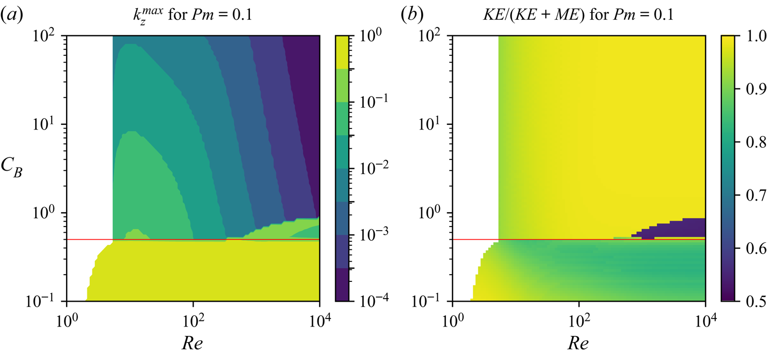
The sinuous KH modes have  $\textrm {Im}[\lambda ] = 0$, and generally have a growth rate
 $\textrm {Re}[\lambda ({k_z^{max}})] \gtrsim 0.1$ for most of the physical parameters where they are found, except when they are nearly stabilized by either magnetic tension or dissipation. The wavenumber where their growth rate peaks is generally in the vicinity of
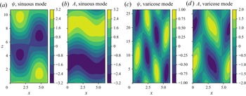
 ${k_z^{max}} \sim 0.5$, as shown in figure 2. Figure 3(a,b) illustrates the structure of the fastest-growing mode (
 $k_z = {k_z^{max}}$) for
 $C_B = 0.1$,
 ${Re} = 100$ and
 ${{{Pm}}} = 0.1$. Figure 3(a) shows the contours of the streamfunction, representing streamlines of flow, and figure 3(b) shows contours of the flux function, representing magnetic field lines. Here,
 $\psi$ and
 $A$ are the spatial structure of the eigenmodes, obtained by solving (2.14) and (2.15) for
 $\psi _n$ and
 $A_n$, which are then used to compute
 $\psi = \textrm {Re}[ \exp (\textrm {i} k_z z) \sum _n \psi _n \, \textrm {e}^{\textrm {i} n x} ]$ (and likewise for
 $A$). The amplitude is normalized such that the total energy of the mode (defined below) is
 $1$. The structure of
 $\psi$, as expected, resembles that of a hydrodynamic KH mode. The perturbations take the form of alternating clockwise and counterclockwise recirculating eddies tilted against the mean shear. The dominant shearwise wavenumbers can be gleaned from the figure and include
 $n = 0$ (driving a mean shearwise flow, as discussed above) and
 $n = \pm 1$; higher-order wavenumbers are present as well, but not as prominent.
(a) Wavenumber of the fastest-growing mode,  ${k_z^{max}}$, as a function of
 ${Re}$ and
 $C_B$ for
 ${{{Pm}}} = 0.1$. (b) Kinetic energy (KE) as a fraction of total energy (
 $\textrm {KE}+\textrm {ME}$) for the fastest-growing mode. Note that the colourbar ranges from 0.5 to 1 – the fraction never drops below 0.5 for the values shown here. Red horizontal lines indicate
 $C_B = 0.5$.

Mode structures are shown for the fastest-growing sinuous KH mode at  ${{{Pm}}} = 0.1$,
 ${Re} = 10^{2}$,
 $C_B = 0.1$ (a,b) and the fastest-growing varicose KH mode at
 ${{{Pm}}} = 0.1$,
 ${Re} = 10^{3}$,
 $C_B = 0.6$ (c,d). (a,c) Contours of the streamfunction
 $\psi$ and (b,d) contours of the flux function
 $A$. Note that the (streamwise) wavelength of each mode is
 $2 {\rm \pi}/ k_z^{max}$, so the true aspect ratio of the modes is not accurately represented here.

The streamfunction and flux function of the eigenmodes can be used to compute their kinetic energy (KE) and magnetic energy (ME), given in this non-dimensionalization by
 \begin{equation} {\rm KE} = \frac{1}{2}\int {{\rm d}\kern0.7pt x} \int \, {{\rm d}}z \left[ \left( \frac{\partial \psi}{\partial z} \right)^{2} + \left( \frac{\partial \psi}{\partial x} \right)^{2} \right] = \sum_{n={-}N}^{N} (k_z^{2} + n^{2}) |\psi_n|^{2} \end{equation}
and
 \begin{equation} {\rm ME} = \frac{C_B}{2}\int {{\rm d}\kern0.7pt x} \int \, {{\rm d}}z \left[ \left( \frac{\partial A}{\partial z} \right)^{2} + \left( \frac{\partial A}{\partial x} \right)^{2} \right] = C_B \sum_{n={-}N}^{N} (k_z^{2} + n^{2}) |A_n|^{2}. \end{equation}
Using these definitions, we show in figure 2(b) the kinetic energy as a fraction of the total energy for the most unstable mode as a function of  ${Re}$ and
 $C_B$ for
 ${{{Pm}}} = 0.1$. Consistent with their interpretation as being primarily driven by a fundamentally hydrodynamic instability, we see that the kinetic energy of sinuous KH modes is significantly more than half of the total energy across these parameters.
3.2. Varicose KH modes
Another class of unstable modes that also emerges is what we call the ‘varicose’ KH modes hereafter, where the term varicose here is used by analogy with varicose modes in, for example, shear instabilities in jets (Mattingly & Criminale Reference Mattingly and Criminale1972; Drazin & Reid Reference Drazin and Reid1981; Mikhaylov & Wu Reference Mikhaylov and Wu2020), or the instabilities present in the streaky flows generated as part of the self-sustaining process in wall-bounded shear flows (Waleffe Reference Waleffe1995, Reference Waleffe1997). While the varicose KH modes also have  $\textrm {Im}[\lambda ] = 0$, they can be distinguished from the sinuous KH modes because they have no
 $x$-averaged shearwise flow or field, and thus
 $\psi _0 = A_0 = 0$.
The varicose KH modes are only found at sufficiently large  ${Re}$, but did not appear in ideal MHD in any of the cases we tested, nor do they exist in the hydrodynamic limit
 $C_B \rightarrow 0$. In figure 1, the region of parameter space where varicose modes are unstable is marked by hatches going down and to the left. For
 $C_B < 0.5$, they are generally subdominant to sinuous modes; for
 $C_B \geq 0.5$, by contrast, varicose modes persist while sinuous modes are typically stabilized (for sufficiently large
 ${{{Rm}}}$, as described in § 3.1). They are always eventually stabilized for sufficiently large magnetic field, however. Their most unstable wavenumber, shown in figure 2(a), is generally of the order of
 ${k_z^{max}} \sim 0.1$, slightly smaller than for the sinuous KH modes. Figure 2(b) also shows that varicose modes are much closer to equipartition between kinetic and magnetic energy than are sinuous modes.
Figure 3 shows that the structure of varicose modes differs significantly from sinuous modes. In particular, we see that the shearwise length scale of the perturbations is smaller, and dominated by the  $n = \pm 2$ mode for the streamfunction, and the
 $n = \pm 1$ mode for the flux function. The flow contains convergent and divergent regions, consistent with varicose modes in other systems (Mattingly & Criminale Reference Mattingly and Criminale1972; Drazin & Reid Reference Drazin and Reid1981; Mikhaylov & Wu Reference Mikhaylov and Wu2020). While these modes appear (to our knowledge) to be unnoticed in the literature, they are not the focus of this paper, and will be discussed in greater detail in future work.
3.3. Alfvénic Dubrulle–Frisch modes
Contrary to the other modes discussed so far, the third type of unstable modes, called Alfvénic Dubrulle–Frisch modes hereafter, exist for arbitrarily large field strength  $C_B$. They are found for
 ${{{Pm}}} < 1$ and for
 ${Re}$ above a critical value that depends on
 ${{{Pm}}}$. Unlike KH modes, they have non-zero frequencies
 $\textrm {Im}[\lambda ]$, and appear in complex-conjugate pairs at each unstable
 $k_z$. Their phase velocity
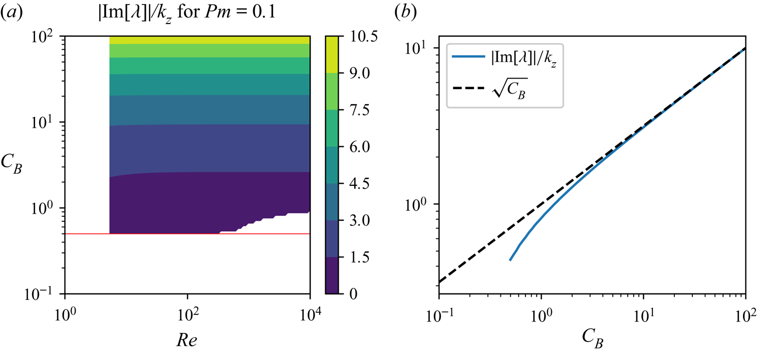
 $\textrm {Im}[\lambda ]/k_z$ scales roughly with the Alfvén velocity
 $\sqrt {C_B}$, as shown in figure 4. Figure 1 shows that their growth rates are much smaller than those of KH modes, and decrease with increasing
 $C_B$. Meanwhile, figure 2 reveals that the fastest-growing modes have much smaller values of
 ${k_z^{max}}$ than KH modes, and that most of the energy is kinetic when
 $Pm\ll 1$.
(a) Phase velocity  $|\textrm {Im}[\lambda ]|/k_z$ of the fastest-growing mode at
 ${{{Pm}}} = 0.1$ as a function of
 $C_B$ and
 ${Re}$, with the horizontal red line indicating
 $C_B = 0.5$. (b) Phase velocity versus
 $C_B$ for
 ${Re} = 100$,
 $Pm = 0.1$. Also shown is the non-dimensional Alfvén velocity
 $\sqrt {C_B}$ for reference.

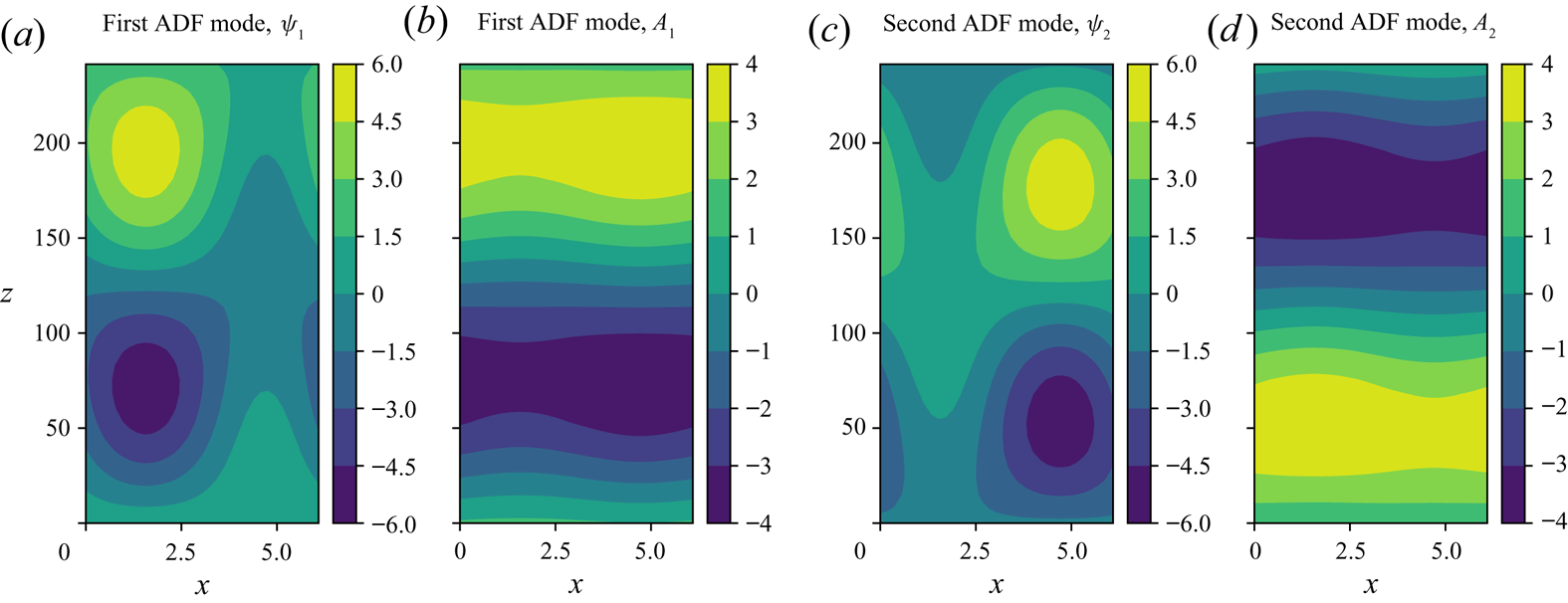
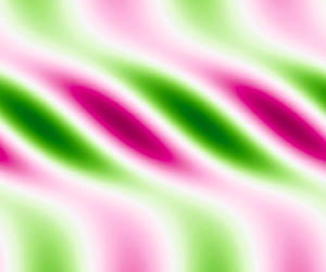
The structure of the fastest-growing Alfvénic Dubrulle–Frisch modes for  ${{{Pm}}} = 0.1$,
 ${Re} = 10^{2}$ and
 $C_B = 1$ is shown in figure 5. We see that, contrary to both the sinuous and varicose KH modes, these unstable waves are highly asymmetric with respect to the background flow profile and behave differently depending on whether
 $\textrm {Im}[\lambda ] > 0$ (i.e. the wave travels downward in the
 $-z$ direction) or
 $\textrm {Im}[\lambda ] < 0$ (i.e. the wave travels upward). More specifically, we see that the downward-travelling perturbations are localized in the upward-moving region of the mean flow, and the upward-travelling perturbations are localized in the downward-moving region of the flow.
Mode structures are shown for the fastest-growing pair of Alfvénic Dubrulle–Frisch (ADF) modes at  ${{{Pm}}} = 0.1$,
 ${Re} = 10^{2}$,
 $C_B = 1$, showing (a,c) contours of
 $\psi$ and (b,d) contours of
 $A$ as in figure 3. (a,b) The mode with
 $\textrm {Im}[\lambda ] > 0$, and thus travelling in the
 $-z$ direction; (c,d) the mode with
 $\textrm {Im}[\lambda ] < 0$ and travelling in the
 $z$ direction. Note that the aspect ratio of the plots does not reflect the aspect ratio of the modes, whose streamwise wavelength
 $2 {\rm \pi}/ k_z$ is much longer than
 $2 {\rm \pi}$, the wavelength of the background flow.

To our knowledge, the Alfvénic Dubrulle–Frisch modes have not been studied elsewhere in the literature. In what follows, we now present a reduced model of these new unstable modes in an effort to characterize them and clarify their origin.
4. Characterizing the Alfvénic Dubrulle–Frisch modes
4.1. A reduced analytical model for the instability
We begin by noting that Alfvénic Dubrulle–Frisch modes have a relatively simple spatial structure (especially at moderate Reynolds numbers) that is well approximated by the most dramatic truncation of (2.9), namely that for  $N = 1$ (where the perturbations only contain a total of three Fourier modes, for
 $n = -1$,
 $n=0$ and
 $n=1$). This is illustrated in figure 6, which compares the growth rate and wavenumber of the fastest-growing mode for truncations at
 $N = 20$,
 $N=5$ and
 $N=1$, respectively, for
 $Re = 100$ and
 $Re = 1000$. In all cases,
 $Pm = Rm/Re = 0.1$, and
 $C_B$ varies between 0.01 and 1000. We see that in general, the
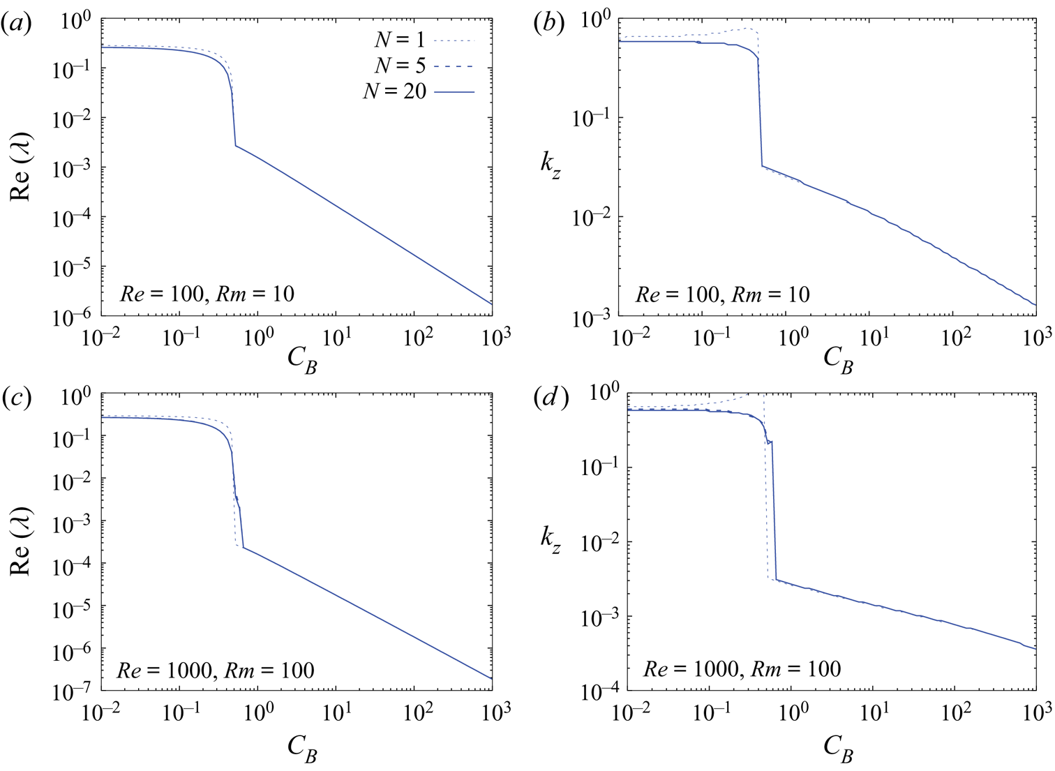
 $N=1$ truncation captures most of the physics of the problem, including the overall amplitude of the growth rate
 $\textrm {Re}(\lambda )$ and wavenumber
 $k_z$ of the fastest-growing mode, and the clear regime transition that happens around
 $C_B = 0.5$. However, we also see that the properties of the Alfvénic Dubrulle–Frisch modes (which are the only modes that exist for
 $C_B \gg 0.5$) are particularly well captured by the
 $N=1$ truncation.
Growth rate  $\textrm {Re}(\lambda )$ (a,c) and wavenumber
 $k_{z}$ (b,d) of the fastest-growing mode of instability as a function of
 $C_B$, for
 $Re = 100$ (a,b) and
 $Re = 1000$ (c,d), for
 $N = 1$ (dotted line),
 $N=5$ (dashed line) and
 $N=20$ (solid line). In all cases
 $Pm = 0.1$. The
 $N=1$ truncation is an excellent approximation to the true system for the Alfvénic Dubrulle–Frisch modes (
 $C_B \gg 0.5$).

With this in mind, we now consider the  $N=1$ truncation only, and restrict our analysis to 2-D modes (so that in (2.8) the sum ranges from
 $n = -1$ to
 $n=1$, and
 $k_y = \tilde {u}_y = 0$). In Appendix B, we demonstrate that in the limit where (1)
 $C_B$ is large and (2)
 $k_z$ is small then
 \begin{equation} {\rm Re}(\lambda) \simeq{-} \frac{ k_z^{2}}{2 } \left(\frac{1}{Re} + \frac{1}{Rm}\right)+ \frac{k_z^{2} \psi_E^{2}}{K^{2}} \frac{Re-Rm}{ 1 + \dfrac{C_B k^{2}_z}{K^{4}} (Rm + Re )^{2} }, \end{equation}
where here  $K^{2} = 1 + k_z^{2}$, and where
 $\psi _E = 1/2$ is the amplitude of the streamfunction associated with the elevator mode
 ${{\boldsymbol u}}_E$. This expression is only valid when
 $C_B \gg 1$, and
 $k_z \ll \min (Re^{-1},Pm,\sqrt {C_B}Rm)$ (see Appendix B for detail), and as a result, does not apply in the inviscid limit (
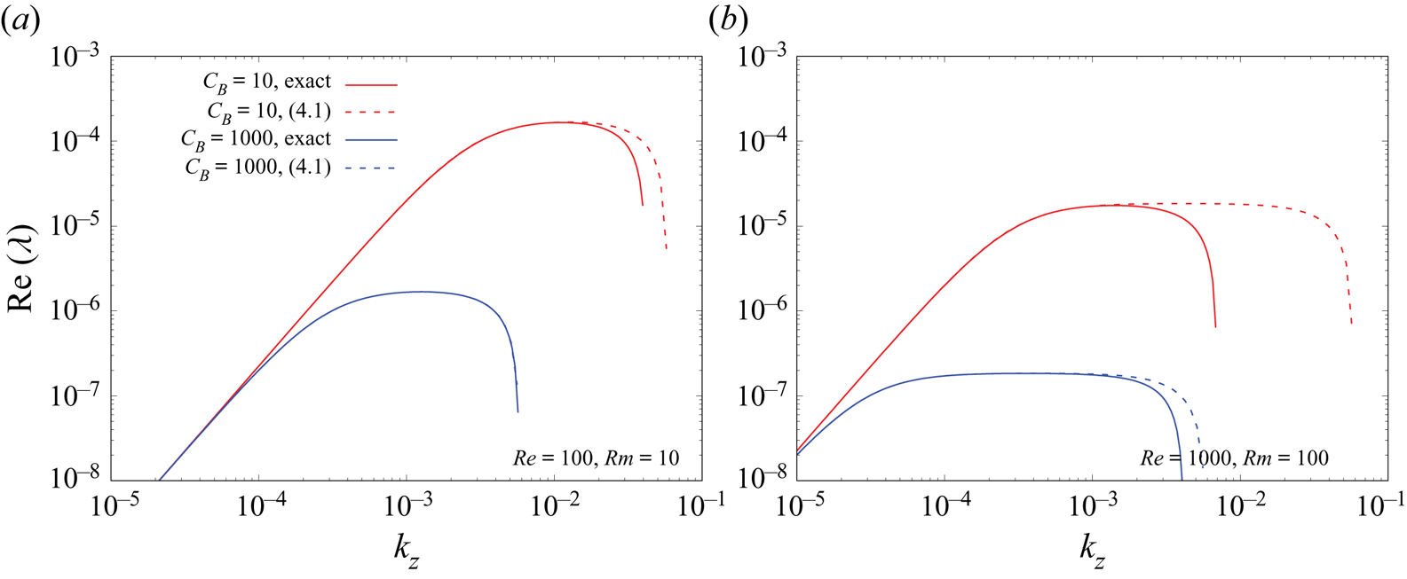
 $Re^{-1} = 0$). Figure 7 compares the prediction of (4.1) with the exact numerical solution of (2.9) for the
 $N=1$ truncation. We see that (4.1) is a good asymptotic approximation to
 $\textrm {Re}(\lambda )$ for small
 $k_z \ll Re^{-1}$ in the limit of large
 $C_B$.


This analytical expression can be used to deduce some of the salient properties of the instability. Crucially, we see that  $\textrm {Re}(\lambda )$ can only be positive when
 $Re > Rm$, or in other words, when
 $Pm < 1$, a result that is consistent with our findings from § 3. Furthermore, a criterion for instability can be obtained by requiring that
 $\textrm {Re}(\lambda )>0$ as
 $k_z \rightarrow 0$, and noting that
 $K^{2} \simeq 1$ in that limit, we find that unstable modes exist provided
 \begin{equation} Re Rm \frac{Re-Rm}{Re+Rm} > 2, \end{equation}
or equivalently,
 \begin{equation} Re > \sqrt{\frac{2}{Pm} \frac{1+Pm}{1-Pm}} \quad \mbox{(for } Pm < 1).\end{equation}
This criterion correctly accounts for the mininum Reynolds number needed for the Alfvénic Dubrulle–Frisch modes to exist in figure 1 (vertical red line). It also shows that the instability is suppressed as  $Pm \rightarrow 1$ from below.
Finally, we can use (4.1) to find the fastest-growing mode for fixed input parameters  $Re$,
 $Rm$ and
 $C_B$, by maximizing
 $\textrm {Re}(\lambda )$ with respect to
 $k_z$. We obtain
 \begin{equation} {k_z^{max}} \simeq{\pm} \frac{1}{\sqrt{C_B}(Rm+Re)} \left( \sqrt{\frac{ReRm}{2} \frac{Re-Rm }{ Re+Rm }} -1 \right)^{1/2},\end{equation}
after assuming that  $K^{2} \simeq 1$ on the basis that
 $k_z$ is small (which can be verified a posteriori).
We see that for moderate  $Re$,
 ${k_z^{max}} = O(C_B^{-1/2} Re^{-1/2})$. Since (4.1) is valid for any
 $k_z \ll 1/Re$ (see Appendix B), (4.4) is then expected to be valid only when
 $C_B \gg Re$. When
 $C_B$ is of order
 $Re$ or less, (4.4) is not valid, and we must instead rely on numerical tools to find
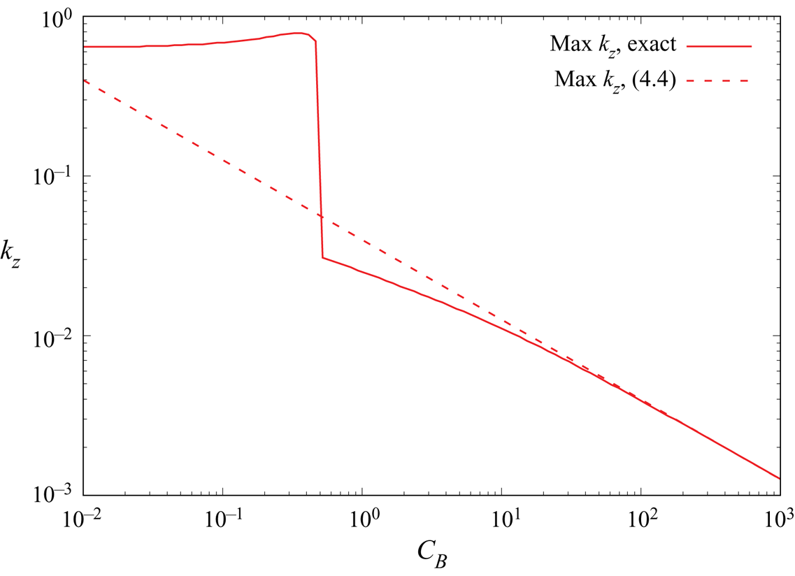
 ${k_z^{max}}$. Figure 8 compares the wavenumber of the fastest-growing mode obtained from (4.4) with
 $Re = 100$ and
 $Rm = 10$ with the one found by maximizing the growth rate obtained numerically over all possible values of
 $k_z$. We see that the approximation is quite good as long as
 $C_B > Re$, as expected from the analysis above.
Fastest-growing mode wavenumber (in the reduced model) at  $Re = 100$,
 $Rm=10$. The solid line shows the numerically determined
 $k_z^{max}$, while the dashed line shows the approximate value estimated from (4.4). The latter is a good approximation to the former for
 $C_B > Re$, as discussed in the main text.

4.2. Interpretation of the results
When written non-dimensionally, (4.1) obfuscates the physics that drive the instability. Dimensionally, however, and using the fact that  $\psi _E=1/2$, we have
 \begin{equation} {\rm Re}(\lambda)^{*} \simeq{-} \frac{ (k_z^{*})^{2}}{2 } ( \nu^{*} + \eta^{*} ) + \frac{(k_z^{*})^{2} (\varPsi^{*})^{2}}{ 4\nu^{*}} \frac{(1-Pm)}{ 1 + \dfrac{(B^{*})^{2} (k_z^{*})^{2}}{\rho_0^{*} \mu_0^{*} (K^{*})^{4}} \left(\dfrac{1}{\nu^{*}} + \dfrac{1}{ \eta^{*}} \right)^{2}},\end{equation}
where  $\varPsi ^{*} = U^{*}/k_x^{*}$ and the asterisk here denotes dimensional quantities. When
 $k^{*}_z$ is sufficiently small (i.e. when the denominator in the second term of (4.5) is approximately equal to
 $1$), then
 $\textrm {Re}(\lambda )^{*} \simeq - D^{*}_{eff} (k_z^{*})^{2}$, with an effective diffusivity given by
 \begin{equation} D^{*}_{eff} = \frac{ 1}{2 } ( \nu^{*} + \eta^{*} ) - \frac{ (\varPsi^{*})^{2}}{ 4\nu^{*}} (1-Pm).\end{equation}
This expression is strongly reminiscent of the results obtained by Dubrulle & Frisch (Reference Dubrulle and Frisch1991) who demonstrated that a purely hydrodynamic sinusoidal flow has an effective viscosity of amplitude
 \begin{equation} \nu^{*}_{eff} = \nu^{*} - \frac{(\varPsi^{*})^{2}}{2\nu^{*}},\end{equation}
when it acts on a large-scale cross-stream flow, which is exactly the situation we have here, albeit in the magnetized case. Note how  $\nu ^{*}_{eff}$ is negative when
 $\varPsi ^{*} > \sqrt {2} \nu ^{*}$, or equivalently, when
 $Re > \sqrt {2}$. In other words, a purely sinusoidal flows has anti-diffusive properties that can serve to amplify a large-scale cross-stream flow. The obvious similarities between (4.6) and (4.7) therefore show that the instability is simply caused by the well-known anti-diffusive properties of the background sinusoidal flow, acting in our case on the slowly decaying Alfvén mode.
As  $k_z^{*}$ increases, the denominator of the second term in (4.5) begins to deviate from 1, which causes the function
 $\textrm {Re}[ \lambda ^{*}(k_z^{*})]$ to flatten (see figure 7) when
 \begin{equation} v_A^{*} k_z^{*} \simeq \frac{\nu^{*}(k_x^{*})^{2} }{1 + Pm } \end{equation}
(where  $v_A^{*}$ is the Alfvén velocity associated with
 $B^{*}$) or equivalently, when the oscillation frequency of the mode becomes of the same order of magnitude as the dissipation rate of
 $n = \pm 1$ component of the mode (although note that the latter is not exactly the right-hand side of this expression, but is of the same order of magnitude). Then, as
 $k_z^{*}$ continues to increase, the second term in (4.5) tends to a constant, and the first term in (4.5), which is negative, gradually takes over to stabilize the mode when
 \begin{equation} v_A^{*} k_z^{*}\simeq k_x^{*} U^{*} \sqrt{\frac{Pm (1-Pm)}{ 2(1 + Pm)^{3} } }, \end{equation}
or in other words, when the oscillation frequency of the mode becomes of the order of the background sinusoidal flow shearing rate (assuming  $Pm$ is not too small). These two thresholds show that (4.6) is only valid in the limit where the oscillation frequency of the mode is much slower than any other characteristic frequency of the system – demonstrating that the oscillatory nature of the shearing Alfvén mode is ultimately detrimental to the Dubrulle–Frisch mechanism. As a result, one can interpret the fastest-growing Alfvénic Dubrulle–Frisch mode (whose non-dimensional wavenumber is approximately given by (4.4)) to be the one whose wavenumber is as large as possible without completely suppressing the Dubrulle–Frisch mechanism.
Realizing that the Dubrulle–Frisch mechanism is at the heart of this magnetized instability also explains why it relies on having a low magnetic Prandtl number. Indeed, in the hydrodynamic limit, long-wavelength cross-stream perturbations are amplified by the Reynolds stresses they create as they distort the background sinusoidal flow. In the magnetized limit, however, Maxwell stresses are necessarily also created by the distortion of the background field, and oppose the Reynolds stresses. A sufficiently large resistivity is therefore needed to soften the effect of the field, so the two kinds of stresses do not cancel out.
Finally it is worth noting that the  $B^{*} \rightarrow 0$ limit of (4.6) does not recover the hydrodynamic limit of Dubrulle & Frisch (Reference Dubrulle and Frisch1991). This is not an inconsistency, as (4.1), and therefore (4.6) as well, are only valid for
 $C_B \gg 1$. However, it is reasonably straightforward to show that
 \begin{equation} {\rm Re}(\lambda^{*}) \simeq{-} (k_z^{*})^{2} \nu^{*}_{eff} \end{equation}
in the reduced model of § 4 when  $C_B = 0$ and
 $k_z \rightarrow 0$, where
 $\nu ^{*}_{eff}$ is given by (4.7), as expected.
5. Numerical simulations
While linear stability analyses can predict the initial response of a fluid in equilibrium to infinitesimal perturbations, they provide no immediate insight into its nonlinear evolution. In this section, we present results from a direct numerical simulation of this system for one set of physical parameters. It is not our intention to perform a comprehensive scan of parameter space, but instead to provide some validation of the linear stability analysis of § 3, and to find out, at least qualitatively, how the Alfvénic Dubrulle–Frisch modes saturate. For this reason, we use the physical parameters  $C_B = 1$,
 ${Re} = 100$ and
 ${{{Pm}}} = 0.1$, ensuring that they are the only unstable modes present in the system (see figure 1).
We use the pseudospectral code Dedalus (Burns et al. Reference Burns, Vasil, Oishi, Lecoanet and Brown2020) to evolve a 2-D version of (2.4) (expressed in terms of a streamfunction  $\psi$ and flux function
 $A$) in time. The simulation is initialized with a unit-amplitude sinusoidal shear flow
 $\boldsymbol {u} = \boldsymbol {u}_E$ and a uniform magnetic field
 $\boldsymbol {b} = {\boldsymbol b}_E = {\boldsymbol e}_z$, i.e. (2.1) and (2.2). We note that this is an equilibrium solution, as the forcing term
 $-{Re}^{-1}\nabla ^{2}\boldsymbol {u}_E$ in (2.4) balances the viscous dissipation of
 $\boldsymbol {u}_E$. We perturb this equilibrium by adding small-amplitude white noise to the streamfunction, which seeds the instability. The simulation uses a domain size of
 $(L_x, L_z) = (4{\rm \pi}, 170{\rm \pi} )$, where the dimensions are chosen to accommodate two wavelengths of the sinusoidal equilibrium in the
 $x$ direction and approximately two wavelengths of the fastest-growing mode, according to the linear stability analysis, in the
 $z$ direction. We note that, even in the hydrodynamic case, the quantitative details of the saturated state of 2-D Kolmogorov flow are expected to depend on domain size and aspect ratio (see, e.g. Lucas & Kerswell (Reference Lucas and Kerswell2014) and references therein). However, for sufficiently large domains, the qualitative properties of the solution ought to be unaffected (a statement which is verified below). The domain is doubly-periodic, with a resolution of 64 Fourier modes in the
 $x$ direction and 256 modes in the
 $z$ direction (for the domain size of
 $(L_x, L_z) = (4{\rm \pi}, 170{\rm \pi} )$ – in simulations where the box size is doubled along an axis, the number of modes in that direction is also doubled to maintain the same resolution). Nonlinear terms are dealiased using the standard 3/2-rule, meaning that nonlinearities are calculated on a
 $92 \times 384$ grid in physical space, and we use a four-stage, third-order, implicit–explicit Runge–Kutta timestepping scheme to evolve the solution in time (Ascher, Ruuth & Spiteri Reference Ascher, Ruuth and Spiteri1997, § 2.8).
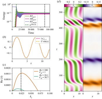
The results are summarized in figure 9. We decompose the flow according to  $\boldsymbol {u} = \langle \boldsymbol {u} \rangle _z + \boldsymbol {u}'$, where
 $\langle \boldsymbol {\cdot } \rangle _z$ denotes an average in
 $z$, and refer to
 $\langle \boldsymbol {u} \rangle _z$ as the mean flow and
 $\boldsymbol {u}'$ as the fluctuating flow, with analogous definitions for the mean and fluctuating magnetic field. Note that the mean flow remains purely
 $z$-directed, i.e.
 $\langle \boldsymbol {u} \rangle _z = \langle u_z \rangle _z \boldsymbol {e}_z$. The kinetic and magnetic energies of the fluctuations are shown alongside the kinetic energy of the mean flow in figure 9(a). As expected, the fluctuations grow early in the simulation at a rate that is consistent with the linear stability results of § 3, shown by the dashed green line. Also consistent with § 3 is the dominance of kinetic energy over magnetic energy of fluctuations in the linear growth phase (see figure 2). Finally, snapshots of the flow and field perturbations at this stage (not shown) are also consistent with those of the unstable modes shown in figure 5.
(a) Kinetic and magnetic energies of perturbations about the mean are shown alongside the kinetic energy of the mean flow for a simulation with  $C_B = 1$,
 ${Re} = 100$ and
 ${{{Pm}}} = 0.1$, with the green dashed line showing the growth rate of the most unstable mode that fits into this domain size according to § 3, demonstrating consistency with the results of that section. (b) The mean flow, averaged in both
 $z$ and
 $t$ (where the time average is taken over the second half of the simulation), is shown with a sine wave overplotted to demonstrate how nearly sinusoidal the flow remains. (c) The dispersion relation based on the initial values of
 ${Re}$ and
 $C_B$ (orange) is shown alongside the dispersion relation based on the values of
 ${Re}_{eff}$ and
 $C_{eff}$ achieved in saturation (green, see text), with the black vertical line showing the wavenumber corresponding to a wavelength that equals the domain height, demonstrating that even in saturation, the mean flow profile remains linearly unstable. (d) A snapshot of
 $u_z$ (left) and
 $u_x$ (right) is shown at
 $t \approx 87\,000$ (indicated by the vertical dashed line in a). At this time, the system is dominated by two counter-propagating solitons that look like dislocations of the mean flow.

The exponential growth phase of the Alfvénic Dubrulle–Frisch modes ends around  $t = 10\,000$, when their amplitudes become commensurate with that of the mean flow. Nonlinear interactions then cause a rapid decrease in the amplitude of the mean sinusoidal flow, from an original value of
 $U = 1$ down to an average of about
 $U = 0.181$; see figure 9(b) (note that repeating the simulation with doubled
 $L_x$ or with doubled
 $L_z$ changes this value to
 $0.180$ or
 $0.191$, respectively). The shape remains almost exactly sinusoidal, however. One may therefore wonder whether, by reducing the mean flow amplitude, the system has simply adjusted itself in such a way as to become marginally stable to all modes of instability, which is a common route towards saturation. To test this idea, we use the new flow amplitude
 $U$ to compute effective Reynolds numbers
 $Re_{eff} = U Re \simeq 18.1$ and
 $Rm_{eff} = U Rm \simeq 1.81$, and an effective magnetic parameter
 $C_{eff} = C_B / U^{2} = 30.7$. Using these effective parameters, we can compute the growth rate of unstable modes on the new background flow, and the results are shown in figure 9(c) (green curve), together with a dashed vertical line indicating the wavenumber of a mode whose wavelength equals the domain height. We clearly see that the system remains unstable to domain-size Alfvénic Dubrulle–Frisch modes, showing that the path to saturation suggested above is not relevant for this simulation.
Furthermore, inspection of the shape and relative amplitude of the flow and field perturbations in the nonlinear state reveals that they are profoundly different from those of linear modes computed in § 3. Indeed, figure 9(d) shows  $u_z$ and
 $u_x$ (including mean and fluctuations) at
 $t \approx 86\,480$, as indicated by the dashed vertical line in the top-left panel. While the unstable modes calculated in § 3 are sinusoidal in
 $z$, the saturated state is dominated by fluctuations that are localized to narrow structures in the
 $z$ direction. These structures appear to be two pairs of counter-propagating solitons, most easily seen in terms of the localized shearwise flows shown in the
 $u_x$ snapshot. The positive-
 $u_x$ fluctuations propagate in the
 $+z$ direction, while the negative-
 $u_x$ fluctuations propagate in the
 $-z$ direction at the same speed, with each soliton unperturbed as it travels through a counter-propagating soliton. We find that the number of solitons remains unchanged when
 $L_x$ is doubled, but that twice as many solitons appear when
 $L_z$ is doubled. Solitons in general have been studied in a range of plasma physics contexts (see, e.g. Ivanov et al. (Reference Ivanov, Schekochihin, Dorland, Field and Parra2020) and references therein). However, the solitons we find here resemble more closely the ‘kinks’ and ‘antikinks’ identified in 2-D hydrodynamic Kolmogorov flows by Lucas & Kerswell (Reference Lucas and Kerswell2014).
Finally, note that we have run many other nonlinear simulations of the Alfvénic Dubrulle–Frisch modes for a variety of input parameters (not shown here). Similar solitons appeared in all cases. The simplicity of these dynamics suggests they may be well described by a low-order dynamical model, similar to that of Lucas & Kerswell (Reference Lucas and Kerswell2014). Such a model, as well as an exploration of how these solitons vary for different physical parameters, domain sizes and 3-D systems, is left to future work.
6. Discussion and conclusion
We have investigated the linear stability of a sinusoidal shear flow with an initially uniform, streamwise magnetic field in 2-D, incompressible MHD with finite viscosity and resistivity. We found three modes of instability, unlike the single KH mode present for this flow in ideal MHD or in the absence of a magnetic field. One of these modes corresponds to the usual KH mode, while the other two modes, to our knowledge, have not been identified elsewhere in the literature. This paper focused on understanding the dynamics of one of these new modes, which we refer to as Alfvénic Dubrulle–Frisch modes. These modes appear as pairs of counter-propagating unstable waves and exist for all magnetic field strengths, but only when the magnetic Prandtl number  ${{{Pm}}} < 1$. By deriving a reduced model for this particular mode of instability, we were able to show that it is amplified by the negative eddy viscosity of periodic shear flows identified by Dubrulle & Frisch (Reference Dubrulle and Frisch1991). Finally, we presented a direct numerical simulation of the nonlinear evolution of these waves, demonstrating that they saturate in a quasi-stationary state dominated by counter-propagating solitons similar to the ‘kinks’ and ‘antikinks’ identified in the hydrodynamic case by Lucas & Kerswell (Reference Lucas and Kerswell2014).
The physical parameters for which this new mode of instability exists lead to two significant consequences worth stressing. First, while the Alfvénic Dubrulle–Frisch modes require finite dissipation (with  ${Re}$ and
 ${{{Rm}}}$ above a certain threshold), we found that they remain unstable no matter how large
 ${Re}$ and
 ${{{Rm}}}$ become, provided
 ${{{Pm}}} < 1$. As a consequence, even when modelling astrophysical plasmas with extreme Reynolds numbers, calculations that employ ideal MHD may erroneously neglect this instability. Second, unlike the ordinary KH mode found in ideal MHD (or its counterpart in this system) which becomes stable for sufficiently strong magnetic fields, the Alfvénic Dubrulle–Frisch modes are unstable for all non-zero magnetic field strengths. Thus, counter to common intuition that shear-flow instabilities are stabilized by parallel magnetic fields of sufficient strength (Chandrasekhar Reference Chandrasekhar1961), our results demonstrate that, at least for the flow profile considered here, instability can persist for arbitrarily large magnetic field strengths. We also note that the Dubrulle–Frisch mechanism applies to periodic shear flows more broadly, not just sinusoidal flows. Thus, we anticipate that these instabilities can be found in other periodic shear flows as well.
As shown in § 4.2, the underlying mechanism for this instability stems from the negative eddy viscosity of periodic shear flows described by Dubrulle & Frisch (Reference Dubrulle and Frisch1991), which amplifies the shear Alfvén waves present in this system in the absence of the background shear flow. The simplicity of this mechanism suggests it might be quite general, and exist in other scenarios where a sinusoidal shear flow is added to a system that naturally supports waves transverse to the mean flow. Indeed, Garaud, Gallet & Bischoff (Reference Garaud, Gallet and Bischoff2015) similarly found low-wavenumber oscillatory modes when studying sinusoidal shear flow in a stratified fluid, which only exist when viscosity is taken into account. While a detailed investigation of these modes was beyond the scope of that work, they appear similar to the ones reported here, with internal gravity waves in that system playing the role of Alfvén waves in the MHD system. We speculate that similar modes might exist in reduced plasma models that permit zonal flows and drift waves (e.g. Zhu, Zhou & Dodin Reference Zhu, Zhou and Dodin2018).
We envision two primary directions for future work based on these results. The first is a thorough investigation of the nonlinear evolution of this instability. We have demonstrated for one set of parameters that this system saturates in a quasi-stationary state that supports counter-propagating solitons. Additional simulations performed over a broad range of physical parameters will be needed to characterize how the speed, number and shape of these solitons vary with input parameters. Furthermore, the simple nature of this saturated state invites efforts to develop reduced nonlinear models of the solitons that can be compared against simulations. Finally, even though we demonstrated that 2-D modes of instability are the fastest-growing ones in the linear regime, it is likely that the saturation of the instability will be profoundly different in two and three dimensions, and it is unclear whether these solitons will persist.
The second direction for future work is to explore the physical implications of these Alfvénic Dubrulle–Frisch modes in magnetized plasmas. As described in § 1, the double-diffusive fingering instability drives ‘elevator’ modes that flow in the vertical direction and vary sinusoidally in the horizontal directions. Their saturation is traditionally modelled by requiring a balance between the finger growth rate, and the growth rate of parasitic shear instabilities (Radko & Smith Reference Radko and Smith2012; Brown et al. Reference Brown, Garaud and Stellmach2013). Harrington & Garaud (Reference Harrington and Garaud2019) (hereafter HG19) recently studied the effect of an added vertical magnetic field, demonstrating both numerically and theoretically that the latter decreases the shear instability growth rate and therefore strongly affects the saturation of the fingering instability. However, all of their simulations were performed with  ${{{Pm}}} = 1$, and their parasitic stability analysis assumed ideal MHD; thus, the effects of Alfvénic Dubrulle–Frisch modes were not present in their simulations or in their reduced model. Since the stellar interiors where fingering convection occurs generally satisfy
 ${{{Pm}}} < 1$, it is possible that the newly discovered modes have an effect on the saturation of magnetized fingering convection that is not accounted for by HG19.
Finally, note that all of the results presented in this paper were obtained for a sinusoidal flow that varies in only one of the two horizontal directions – a planar shear flow – which is the geometry for which the Dubrulle & Frisch (Reference Dubrulle and Frisch1991) mechanism was originally discussed. However, in many of the instabilities discussed above, the primary elevator modes vary sinusoidally along both horizontal axes, as seen in figure 1 of HG19 or discussed in § 3.2 of Radko & Smith (Reference Radko and Smith2012). Furthermore, we have neglected the temperature and compositional fluctuations associated with elevator modes, which likely modify the quantitative details of this instability and its saturation (see Radko & Smith (Reference Radko and Smith2012) for an example where these fluctuations were not neglected). It will therefore be important to establish in future work whether the instability mechanism discovered here remains active for MHD shear flows where the shear varies along two axes, e.g. for flows with structure  $\boldsymbol {u}_E = \sin (x)\sin (y) \boldsymbol {e}_z$, and how it is affected by the temperature and compositional structure of elevator modes when applied to model fingering convection.
Acknowledgements
This work used the Extreme Science and Engineering Discovery Environment (XSEDE) Expanse supercomputer at the San Diego Supercomputer Center through allocation TG-PHY210050. We thank S. Tobias, D. Hughes, P. Terry, E. Zweibel, M.J. Pueschel, N. Hurst, A. Kaminski and J. Oishi for useful conversations.
Funding
A.E.F. and P.G. acknowledge support from National Science Foundation grant AST-1908338. I.G.C. acknowledges the support of the University of Colorado's George Ellery Hale Graduate Student Fellowship. Some of this work was part of a Kavli Summer Program in Astrophysics project, funded by the Kavli Foundation. We acknowledge use of the Lux supercomputer at UC Santa Cruz, funded by NSF MRI grant AST-1828315.
Declaration of interests
The authors report no conflict of interest.
Data availability statement
The simulation data presented here are available upon reasonable request.
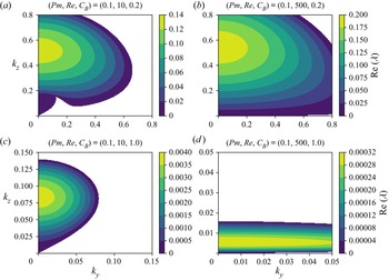
Appendix A. Linear growth rates of 3-D perturbations
Here we demonstrate, for a sample of physical parameters, how the linear growth rate of 3-D perturbations varies with  $k_y$ and
 $k_z$. Figure 10 shows the growth rate
 $\textrm {Re}[\lambda ]$ of 3-D perturbations over a range of
 $k_y$ and
 $k_z$ for
 $Pm = 0.1$ and
 $(Re, C_B) = (10, 0.2)$,
 $(500, 0.2)$,
 $(10, 1)$ and
 $(500, 1)$, while figure 11 shows the growth rate of 3-D perturbations for
 $Pm = 2$ and
 $(Re, C_B) = (10, 0.2)$,
 $(500, 0.2)$ and
 $(500, 0.6)$, corresponding to the magenta diamonds in figure 1. For each set of parameters, we see that the mode with the largest growth rate is a 2-D mode with
 $k_y = 0$. However, we note that the
 $(Pm, Re, C_B) = (0.1, 10, 0.2)$ case presents an example where, for some values of
 $k_z$ (in this case, for
 $k_z \approx 0.2$), there are 3-D modes that grow faster than the corresponding 2-D mode – though it remains true that the fastest-growing mode is 2-D.
Growth rates  $\textrm {Re}[\lambda ]$ of 3-D perturbations across a range of
 $k_y$ and
 $k_z$ for
 $Pm = 0.1$. The 2-D modes considered in the majority of the main text correspond to
 $k_y = 0$. Each panel shows growth rates for a different set of physical parameters as indicated by the magenta diamonds in figure 1. For each set of physical parameters, the fastest-growing mode is 2-D.

As in figure 10, but for  $Pm = 2$. Once again, in each case, the fastest-growing mode is 2-D for each set of physical parameters.

Appendix B. Asymptotic approximation of the growth rate of Alfvénic Dubrulle– Frisch modes
To gain a better understanding of the nature of the Alfvénic Dubrulle–Frisch modes, we now seek approximate analytical solutions of (2.9) in the limit of large  $C_B$. For this purpose, we choose a new non-dimensionalization for the governing equations that better accounts for the mode dynamics. In what follows, and for the rest of this appendix, we now use the Alfvén velocity
 \begin{equation} v_A^{*} = \frac{B^{*}}{\sqrt{\rho_0^{*} \mu_0^{*}}} \end{equation}
as the unit velocity, and continue to use  $(k_x^{*})^{-1}$ as the unit length and
 $B^{*}$ as the unit magnetic field. The unit time is then
 $(v_A^{*} k_x^{*})^{-1}$. In this new set of units, the governing equations are
 \begin{equation} \left.\begin{array}{c@{}}
\displaystyle \dfrac{\partial {{\boldsymbol u}}}{\partial
t} + {{\boldsymbol u}} \boldsymbol{\cdot}
\boldsymbol{\nabla} {{\boldsymbol u}} ={-}
\boldsymbol{\nabla} p + (\boldsymbol{\nabla} \times
{{\boldsymbol b}}) \times {{\boldsymbol b}} +
{{{Pm}}}S^{{-}1} \nabla^{2} ({{\boldsymbol
u}}-{{\boldsymbol u}}_E), \\ \displaystyle \dfrac{\partial
{\boldsymbol b}}{\partial t} = \boldsymbol{\nabla} \times
({\boldsymbol u} \times {\boldsymbol b}) + S^{{-}1}
\nabla^{2} {\boldsymbol b}, \\ \boldsymbol{\nabla}
\boldsymbol{\cdot} {{\boldsymbol u}} = 0 , \quad
\boldsymbol{\nabla} \boldsymbol{\cdot} {{\boldsymbol b}} =
0, \end{array}\right\} \end{equation}
and the background sinusoidal flow is
 \begin{equation} {{\boldsymbol u}}_E = \frac{U^{*}}{v_A^{*}} \sin(x) {\boldsymbol e}_z = C_B^{{-}1/2} \sin(x) {\boldsymbol e}_z . \end{equation}
We see that this choice of units has introduced a new non-dimensional number, namely the Lundquist number:
 \begin{equation} S = \frac{v_A^{*}}{\eta^{*} k_x^{*}} = \sqrt{C_B} Rm, \end{equation}
which is usually interpreted as the ratio of an Alfvénic oscillation frequency  $k_x^{*} v_A^{*}$ with a magnetic diffusion rate
 $\eta ^{*} (k_x^{*})^{2}$.
The  $N=1$ truncation of the Fourier mode expansion discussed in § 4 is equivalent to seeking solutions for the streamfunction
 $\psi$ and the flux function
 $A$ of the kind
 $$\begin{gather} \psi(x,z,t) = {\rm e}^{\lambda t + {\rm i}k_z z} ( \psi_0 + \psi_1 {\rm e}^{{\rm i} x } + \psi_{{-}1} {\rm e}^{-{\rm i} x } ) , \end{gather}$$
 $$\begin{gather}A(x,z,t) = i {\rm e}^{\lambda t+{\rm i}k_z z} ( a_0 + a_1 {\rm e}^{{\rm i} x } + a_{{-}1} {\rm e}^{-{\rm i} x } ). \end{gather}$$
Note that the added factor of  $i$ in the expression for
 $A$ (so
 $ia_n = A_n$ for all
 $n$) makes the coefficients in the resultant system shown below real, which is both convenient and without loss of generality. The first term in each definition (terms in
 $\psi _0$,
 $a_0$) corresponds to
 $x$-invariant modes, sometimes referred to as ‘shearing modes’ hereafter, while the second and third terms correspond to inclined modes that have structure in both shearwise (
 $x$) and streamwise (
 $z$) directions.
Substituting this ansatz into (2.12) and (2.13), expressed in the new units, and projecting onto the relevant Fourier modes, yields the linear system
 \begin{equation} \left.\begin{array}{c@{}}
\displaystyle \left( \lambda + Pm\dfrac{k_z^{2} }{S}
\right) \psi_0 - \dfrac{1}{2\sqrt{C_B}} k_z ( \psi_{1} -
\psi_{{-}1}) ={-} k_z a_0 , \\ \displaystyle \left( \lambda
+ Pm\dfrac{K^{2} }{S} \right) \psi_1 -
\dfrac{1}{2\sqrt{C_B}} k_z \dfrac{1 - k_z^{2}}{ K^{2}}
\psi_0 ={-} k_z a_1 , \\ \displaystyle \left( \lambda + Pm
\dfrac{K^{2}}{S} \right) \psi_{{-}1} +
\dfrac{1}{2\sqrt{C_B}} k_z \dfrac{1 - k_z^{2}}{ K^{2}}
\psi_0 ={-} k_z a_{{-}1} , \\ \displaystyle \left( \lambda
+ \dfrac{k_z^{2}}{S} \right) a_0 = k_z \psi_0 -
\dfrac{1}{2\sqrt{C_B}} k_z ( a_{{-}1} - a_1 ) , \\
\displaystyle \left( \lambda + \dfrac{K^{2}}{S} \right) a_1
= k_z \psi_1 - \dfrac{1}{2\sqrt{C_B}} k_z a_0 , \\
\displaystyle \left( \lambda + \dfrac{K^{2} }{S} \right)
a_{{-}1} = k_z \psi_{{-}1} + \dfrac{1}{2\sqrt{C_B}} k_z
a_0, \end{array}\right\}
\end{equation}
where  $K^{2} = 1 + k_z^{2}$.
Note that if we look at the limit of extremely strong field and negligible diffusivity (i.e.  $C_B, S \rightarrow \infty$), the system reduces to
 \begin{equation} \left.\begin{array}{c@{}}
\lambda \psi_0 ={-} k_z a_0, \quad \lambda a_0 = k_z
\psi_0, \\ \lambda \psi_1 ={-} k_z a_1, \quad \lambda a_1 =
k_z \psi_1, \\ \lambda \psi_{{-}1} ={-} k_z a_{{-}1}, \quad
\lambda a_{{-}1} = k_z \psi_{{-}1}, \end{array}\right\}
\end{equation}
so that  $\lambda ^{2} q = - k_z^{2} q$ for
 $q \in \{ \psi _0, \psi _1, \psi _{-1}, a_0, a_1, a_{-1} \}$. Each of these leads to
 $\lambda = \pm \textrm {i} k_z$, which is the non-dimensional version of the dispersion relationship for non-dissipative Alfvén waves travelling on a constant streamwise magnetic field, which is as expected in the limit considered. But we also see that in this limit, the modes do not grow.
Going back to (B7) for finite values of  $C_B$ and
 $S$, and taking the sum of the
 $\psi _1$ and
 $\psi _{-1}$ equations, and the sum of the
 $a_{-1}$ and
 $a_1$ equations, we obtain the reduced system
 \begin{equation} \left.\begin{array}{c@{}}
\displaystyle \left( \lambda + Pm \dfrac{K^{2} }{S} \right)
(\psi_1 + \psi_{{-}1}) ={-} k_z ( a_1 + a_{{-}1}), \\
\displaystyle \left( \lambda + \dfrac{K^{2} }{S} \right) (
a_1 + a_{{-}1}) = k_z (\psi_1 + \psi_{{-}1}).
\end{array}\right\} \end{equation}
This shows that, for modes with  $a_1 + a_{-1}\neq 0$ and
 $\psi _1 + \psi _{-1} \neq 0$,
 $\lambda$ satisfies the simple quadratic equation
 \begin{equation} \left( \lambda + Pm \frac{K^{2} }{S} \right) \left( \lambda + \frac{K^{2} }{S} \right) ={-} k_z^{2},\end{equation}
whose solutions are
 \begin{equation} \lambda ={-} \frac{K^{2} }{2S} ( Pm + 1 ) \pm {\rm i} k_z \sqrt{ 1- \frac{K^{4} }{4S^{2}k_z^{2}} ( Pm- 1 )^{2}} . \end{equation}
These correspond to viscously and resistively damped Alfvén waves that decay on the time scale of order  $S/K^{2}$ (in the selected units), with
 $K$ of order unity. This result implies that the system dynamics relaxes to the subset of eigenmodes for which
 $a_1 =-a_{-1}$, and
 $\psi _1 = - \psi _{-1}$, on a relatively short time scale (unless
 $S$ is very large).
To look outside of this strictly decaying subspace (since we are looking for growing modes), we then assume  $a_1 =-a_{-1}$, and
 $\psi _1 = - \psi _{-1}$ in (B7), and obtain the new reduced system
 \begin{equation} \left.\begin{array}{c@{}}
\displaystyle \left( \lambda + Pm\dfrac{k_z^{2} }{S}
\right) \psi_0 = \dfrac{1}{\sqrt{C_B}} k_z \psi_{1} - k_z
a_0 , \\ \displaystyle \left( \lambda + Pm\dfrac{K^{2}}{S}
\right) \psi_{1} = \dfrac{1}{2\sqrt{C_B}} k_z \dfrac{1 -
k_z^{2}}{ K^{2}} \psi_0 - k_z a_1 , \\ \displaystyle \left(
\lambda + \dfrac{k_z^{2}}{S}\right) a_0 = k_z \psi_0 +
\dfrac{1}{\sqrt{C_B}} k_z a_1 , \\ \displaystyle \left(
\lambda + \dfrac{K^{2} }{S} \right) a_1 = k_z \psi_{1} -
\dfrac{1}{2\sqrt{C_B}} k_z a_0. \end{array}\right\}
\end{equation}
It can be shown with a little algebra that this yields a quartic equation for the eigenvalue  $\lambda$:
 \begin{align} &\left(\lambda + Pm\frac{K^{2}}{S}\right)\left(\lambda+ Pm\frac{ k_z^{2}}{S}\right)\left(\lambda+ \frac{K^{2}}{S}\right) \left(\lambda + \frac{ k_z^{2}}{S} \right)\nonumber\\ &\qquad + k^{2}_z \left[ \left(\lambda+ \frac{K^{2}}{S}\right) \left(\lambda + Pm\frac{K^{2}}{S}\right) + \left(\lambda+ Pm \frac{ k_z^{2}}{S}\right)\left(\lambda + \frac{ k_z^{2}}{S} \right) \right] \nonumber\\ &\qquad - \frac{1}{2C_B} k_z^{2} \frac{1 - k_z^{2}}{ K^{2}} \left(\lambda+ \frac{K^{2}}{S}\right) \left(\lambda+ \frac{k_z^{2}}{S}\right) + \frac{1}{2C_B} k_z^{2} \left(\lambda + Pm\frac{K^{2}}{S}\right)\left(\lambda + Pm\frac{k_z^{2}}{S}\right)\nonumber\\ &\quad = k^{4}_z \left[ - 1 + \frac{1}{C_B} \frac{k_z^{2}}{ K^{2}} + \frac{1}{4C_B^{2} } \frac{1 - k_z^{2}}{ K^{2}} \right] . \end{align}
Since we are looking for solutions at large magnetic field strengths ( $C_B \gg 1$), we now introduce the small parameter
 $\epsilon = C_B^{-1}$, and assume an asymptotic expansion of the kind
 $\lambda = \lambda _0 + \epsilon \lambda _1$ (which will be verified a posteriori to be correct). In the limit
 $\epsilon =0$, (B13) reduces to two possible quadratic equations in
 $\lambda _0$, namely the equations for the decay rates of diffusive Alfvén waves:
 \begin{equation} \left.\begin{array}{c@{}}
\displaystyle \left(\lambda_0+ \dfrac{K^{2}}{S}\right)
\left(\lambda_0 + Pm\dfrac{K^{2}}{S}\right) + k_z^{2} = 0,
\\ \displaystyle \left(\lambda_0+ Pm\dfrac{
k_z^{2}}{S}\right)\left(\lambda_0 + \dfrac{ k_z^{2}}{S}
\right) + k_z^{2} = 0. \end{array}\right\}
\end{equation}
The first one is identical to (B10), and was discarded on the basis that the corresponding modes decay too rapidly. We continue to discard it here, as it would lead to modes that do not grow. The second one has solutions that decay on the time scale  $O(S/k^{2}_z)$, which can be very long provided
 $k_z$ is sufficiently small. These are given by
 \begin{equation} \lambda_0 ={-} \frac{ k_z^{2}}{2S} ( Pm+ 1 ) \pm {\rm i} k_z \sqrt{ 1 - \frac{k_z^{2}}{4S^{2}} ( 1-Pm )^{2}}.\end{equation}
The corresponding modes are pure ‘shearing’ Alfvén modes in the terminology introduced earlier, i.e. at lowest order their velocity field is invariant in the shearwise direction. As we demonstrate, it is the interaction of these modes with the background shear that drives the growth of Alfvénic Dubrulle–Frisch modes.
Expanding (B13) to first order in  $\epsilon$, and using (B14) and (B15), we find that the first-order correction
 $\lambda _1$ satisfies the linear equation
 \begin{align} &\lambda_1 \left(2 \lambda_0 + (Pm+1) \frac{ k_z^{2}}{S}\right) \left[ \left(\lambda_0 + Pm\frac{K^{2}}{S}\right)\left(\lambda_0 + \frac{K^{2}}{S}\right) + k^{2}_z \right] \nonumber\\ &\quad = \frac{k_z^{6}}{ K^{2}} + \frac{1}{2} k_z^{2} \frac{1 - k_z^{2}}{ K^{2}} \left(\lambda_0 + \frac{K^{2}}{S}\right) \left(\lambda_0 + \frac{k_z^{2}}{S}\right) - \frac{1}{2} k_z^{2} \left(\lambda_0 + Pm\frac{K^{2}}{S}\right)\left(\lambda_0 + Pm\frac{k_z^{2}}{S}\right). \end{align}
Every term in this equation is known, so  $\lambda _1$ can easily be calculated. Unfortunately, even though this expression is analytical, it is not particularly illuminating. In what follows, we now aim to obtain a much simpler analytical expression, at least in some region of parameter space, that will allow us to gain a better understanding of the nature of the instability. To do so, we capitalize on the fact that the Alfvénic Dubrulle–Frisch modes have a very small wavenumber (see § 3), and further expand both
 $\lambda _0$ and
 $\lambda _1$ in the limit of
 $k_z \rightarrow 0$. Keeping only terms of lowest order in
 $k_z$, we have
 \begin{equation} \lambda_0 \simeq{-} \frac{ k_z^{2}}{2S} ( Pm+ 1 ) \pm {\rm i} k_z ,\end{equation}
and after some cumbersome but otherwise straightforward algebra,
 \begin{equation} \lambda_1 \simeq \frac{S (1-Pm) k_z^{2}}{4 Pm K^{2} \left[ 1 + S^{2} \dfrac{k_z^{2}}{K^{4}} \left( \dfrac{Pm+1}{Pm} \right)^{2} \right] } \left[ 1 \mp i S \frac{k_z}{K^{2}} \frac{Pm+1}{Pm} \right],\end{equation}
where we have had to assume that  $k_z \ll S$,
 $k_z \ll Pm$ and
 $S^{2}\gg Pm$.
For the Taylor expansion of the complex growth rate  $\lambda$ in the small parameter
 $\epsilon$ to be meaningful, one needs to ensure that
 $\epsilon |\lambda _1| \ll |\lambda _0|$, which is equivalent to requiring that both
 $\epsilon |\textrm {Re}(\lambda _1)| \ll | \lambda _0|$ and
 $\epsilon |\textrm {Im}(\lambda _1)| \ll |\lambda _0|$. With
 $|\lambda _0| \sim O(k_z)$, and noting that the second constraint turns out to be more stringent than the first, we obtain the condition
 \begin{equation} k^{2}_z \ll C_B \frac{4 Pm^{2} } {S^{2} (1-Pm^{2})} \rightarrow k_z = o(Re^{{-}1}), \end{equation}
noting that  $Pm^{2} C_B / S^{2} = 1/Re^{2}$, and assuming that
 $Pm$ is not too close to 1. For values of
 $k_z$ approaching
 $O(Re^{-1})$ the expansion is no longer strictly valid, but remains adequate, which explains the trends seen in figure 7 in the main text. Finally, we can substitute this expression and the one for
 $\lambda _0$ into
 $\lambda = \lambda _0 + \epsilon \lambda _1$ to obtain an approximate expression for the real part of
 $\lambda$:
 \begin{equation} {\rm Re}(\lambda) \simeq{-} \frac{ k_z^{2}}{2S} ( Pm+ 1 ) + \frac{1}{C_B} \frac{S (1-Pm) k_z^{2}}{4 Pm K^{2} \left[ 1 + S^{2} \dfrac{k_z^{2}}{K^{4}} \left( \dfrac{Pm+1}{Pm} \right)^{2} \right] } , \end{equation}
which, once expressed in the units of the main body of the paper, becomes (4.1). This expression is valid provided
•
$C_B \gg 1$,•
$k_z \ll \min (Re^{-1},Pm,S)$ and•
$S^{2} \gg Pm$,


which incidentally shows that it does not apply in the inviscid limit. A similar derivation for the true inviscid case ( $Pm = 0$, or equivalently
 $Re^{-1} = 0$ with finite
 $Rm$) yields negative values for both
 $\textrm {Re}(\lambda _0)$ and
 $\textrm {Re}(\lambda _1)$, revealing that the long-wavelength (small
 $k_z$), large-
 $C_B$ limit is only unstable in the presence of viscosity.