2.1. Variational formulation for gravity-capillary waves

We introduce the Cartesian coordinate system, where $x$ is the horizontal coordinate, and $y$ denotes the vertical direction, with $y=0$ corresponding to the undisturbed free surface. We consider a two-dimensional, inviscid and incompressible fluid of finite depth $h_0$ that flows irrotationally. In this case, the velocity field of the fluid can be expressed as the gradient of a potential function $\phi (x,y,t)$ , where $t$ represents time. According to Luke (Reference Luke1967), the free-surface water-wave system follows completely from minimising the action $\iint L\,{\rm d}x\,{\rm d}t$ with the Lagrangian

(2.1) \begin{align} L=\int _{-h_0}^{\eta }\left (\phi _t+\frac 12\phi _x^2+\frac 12\phi _y^2+gy\right ){\rm d}y+\frac {\sigma }{\rho }\left (\sqrt {1+\eta _x^2}-1\right )\!, \end{align}

where $y=\eta (x,t)$ is the free-surface displacement, $\sigma$ is the surface tension coefficient, $\rho$ is the fluid density, and $g$ is the acceleration due to gravity. Perturbing the Lagrangian action by $\delta \phi$ yields

(2.2) \begin{align} \begin{aligned} \phi _{xx}+\phi _{yy}=0\quad &\text{for}\ {-h_0}\lt y\lt \eta ,\\ \eta _t+\eta _x \phi _x-\phi _y=0\quad &\text{at}\ y=\eta ,\\ \phi _y=0\quad &\text{at}\ y=-h_0. \end{aligned} \end{align}

On the other hand, taking the variational derivative with respect to $\eta$ gives

(2.3) \begin{align} \phi _t+\frac 12\big (\phi _x^2+\phi _y^2\big )+g\eta -\frac {\sigma }{\rho }\partial _x\left (\frac {\eta _x}{\sqrt {1+\eta _x^2}} \right )=0\quad \text{at}\ y=\eta . \end{align}

The governing equation and boundary conditions in (2.2) and (2.3) constitute a complete system for the two-dimensional free-surface water-wave problem, with gravity and surface tension as the restoring forces. For ease of notation, we define $\tau =\sigma /\rho$ as the ratio of the surface tension coefficient to fluid density in the subsequent analyses. We introduce two important dimensionless numbers: the (inverse) Bond number $B$ , and the Froude number $ \textit{Fr} $ . These parameters will be referenced throughout the remainder of this work. They are defined as

(2.4) \begin{align} B=\frac {\tau }{gh_0^2},\quad \textit{Fr} = \frac {c}{\sqrt {gh_0}}, \end{align}

where $c$ represents the wave speed.

2.2. The averaged variational principle for periodic waves

The Whitham modulation theory provides a powerful analytic tool for investigating slowly varying periodic wavetrains (Whitham Reference Whitham1967, Reference Whitham1999). It can be derived generically by averaging dispersive hydrodynamic conservation laws for nonlinear periodic travelling waves to generate first-order dispersionless PDEs of hyperbolic or elliptic type. The averaged Lagrangian approach is standard, and its application to gravity-capillary waves can be partly found in Easwaran (Reference Easwaran1986). For the completeness of the paper, we briefly describe the derivation of the Whitham modulation equations. Interested readers are referred to Whitham (Reference Whitham1967) and Easwaran (Reference Easwaran1986) for more details.

The essence of the averaged Lagrangian approach is that the amplitude, frequency or wavenumber of modulated waveforms varies on a scale that is significantly larger than the wavelength of the oscillations. Therefore, by averaging over the rapid oscillations, we can derive governing equations for the slowly varying parameters. The most general form for a periodic wavetrain can be expressed as

(2.5) \begin{align} \phi =\psi +\varPhi (\theta ,y),\quad \eta =N(\theta ), \end{align}

where $\varPhi$ and $N$ are periodic functions of $\theta$ . In this context, $\theta$ and $\psi$ are the fast phases that satisfy

(2.6) \begin{align} \theta _x=k,\quad \theta _t=-\omega ,\quad \psi _x=\beta ,\quad \psi _t=-\gamma , \end{align}

where $k$ , $\omega$ , $\beta$ and $\gamma$ are slowly varying quantities. Specifically, $k$ represents the wavenumber, $\omega$ indicates the frequency, $\beta$ denotes the mean horizontal velocity, and $\gamma$ relates to absorbing the Bernoulli constant into the potential. It follows immediately that

(2.7) \begin{align} \frac {\partial k}{\partial t}+\frac {\partial \omega }{\partial x}=0,\quad \frac {\partial \beta }{\partial t}+\frac {\partial \gamma }{\partial x}=0. \end{align}

In the expression of the wave profile $N$ , two additional parameters must be specifically considered: the mean amplitude of the wave, $a$ , and the mean height, $b$ , defined respectively as

(2.8) \begin{align} a=\frac {1}{\pi }\int _0^{2\pi }N(\theta )\cos (\theta )\,{\rm d}\theta ,\quad b=\frac {1}{2\pi }\int _0^{2\pi }N(\theta )\,{\rm d}\theta . \end{align}

The Stokes expansion for a uniform wavetrain is expressed in powers of $ka$ . While the series is not uniformly valid as $kh_0\rightarrow 0$ , $ka$ must remain small compared to $(k h_0)^3$ in that limit. This expansion is derived from the Fourier series

(2.9) \begin{align} \begin{aligned} &N(\theta )=b+a\cos \theta +\sum _{n=2}^{\infty }a_n\cos (n \theta ),\\&\varPhi (\theta ,y)=\sum _{n=1}^{\infty }\frac {A_n}{n}\cosh \left (nk(h_0+y)\right )\sin (n\theta ). \end{aligned} \end{align}

Under the short-wave assumption, it requires that $ka_n$ and $kA_n$ are $O(\epsilon ^n)$ , with $\epsilon$ representing a typical value of $ka$ .

The quantities $k$ , $\omega$ , $\beta$ , $\gamma$ , $a$ , $b$ , $a_n$ and $A_n$ are all considered to be slowly varying functions of space and time, and the relations among these quantities can be derived from an averaged form of the variational principle. The general approach involves replacing the averaged Lagrangian over one wavelength in (2.1), then using the variational principle to derive the modulation equations, namely

(2.10) \begin{align} 0=\delta \int _{t_1}^{t_2}\int _{-\infty }^{\infty }\mathscr{L}\,{\rm d}x\,{\rm d}t,\quad \text{with}\ \mathscr{L} = \frac {1}{2\pi }\int _0^{2\pi }L\,{\rm d}\theta . \end{align}

The variations with respect to $A_1$ and $A_2$ , $\mathscr{L}_{A_1}=\mathscr{L}_{A_2}=0$ , provide expressions for $A_1$ and $A_2$ in terms of other unknown quantities, while the variation with respect to $a_2$ yields the relation between $a_2$ and $a$ . Therefore, we can rewrite the average Lagrangian expression, valid up to $O(\epsilon ^4)$ , as

(2.11) \begin{align} \mathscr{L}=\left (\frac {1}{2}\beta ^2-\gamma \right )h+\frac {g}{2}b^2+\frac {E}{2}\left [1-\frac {(\omega -\beta k)^2}{kT \! \left(g+\tau k^2 \right)}\right ]+\frac {E^2k^2D_0}{2 \!\left (g+\tau k^2\right )}+O(\epsilon ^6), \end{align}

where

(2.12) \begin{gather} h=h_0+b,\quad E=\frac {1}{2}\big(g+\tau k^2 \big)a^2,\quad T=\tanh (k h),\quad T_0=\tanh (k h_0),\nonumber \\ D_0=\frac {g^2 \!\left (9 T_0^4-10 T_0^2+9\right )+gk^2\tau \! \left (15 T_0^4-44 T_0^2+30\right )+k^4\tau ^2 \! \left (6T_0^4-25 T_0^2+21\right )}{8T_0\big(g+\tau k^2 \big)\left [gT_0^2+k^2\tau \left (T_0^2-3\right )\right ]}. \end{gather}

The variation with respect to $a$ , or equivalently $E$ , enables the approximation of the nonlinear dispersion relation up to $O(\epsilon ^2)$ :

(2.13) \begin{align} \omega =\omega _0+k\beta +k\left [c_g-\frac 12\left (1+\frac {2k^2\tau }{g+k^2\tau }\right )c_p\right ]\frac {b}{h_0}+D_0\frac {k^2 E}{c_p}+O(\epsilon ^4), \end{align}

where $b$ and $\beta$ are taken to be $O(\epsilon ^2)$ , and

(2.14) \begin{align} \omega _0^2=k \tanh (kh_0)\,\big(g+\tau k^2 \big), \quad c_p=\frac {\omega _0}{k},\quad c_g=\frac {c_p}{2}\left [1+\frac {2\tau k^2}{g+\tau k^2}+\frac {2kh_0}{\sinh (2kh_0)}\right ]\!. \end{align}

Furthermore, the variation with respect to the mean surface height $b$ , $\mathscr{L}_b=0$ , illustrates the relationship between $\gamma$ , $\beta$ and $b$ , expressed as

(2.15) \begin{align} \gamma =\frac {1}{2}\beta ^2+gb+\frac 12\left [\frac {2c_g}{c_p}-\left (1+\frac {2k^2\tau }{g+k^2\tau }\right )\right ]\frac {E}{h_0}+O(\epsilon ^4). \end{align}

Finally, taking the variational derivatives of the action with respect to $\theta$ and $\psi$ yields

(2.16) \begin{align} \frac {\partial }{\partial t}\left (\frac {E}{\omega _0}\right )+\frac {\partial }{\partial x}\left (c_g\frac {E}{\omega _0}\right )=0,\quad \frac {\partial h}{\partial t}+\frac {\partial }{\partial x}\left (\beta h+\frac {E}{c_p}\right )=0. \end{align}

Equations (2.7) and (2.16) form a closed first-order PDE system, where $\omega$ and $\gamma$ are given by (2.13) and (2.15), respectively. It is important to note that the first equation in (2.16) corresponds to the physical principle of wave action conservation. In this context, $E/\omega _0$ represents the wave action, as described by Grimshaw (Reference Grimshaw1975).

As suggested by Whitham (Reference Whitham1999), we can rearrange (2.7) and (2.16) using Noether’s theorem to reveal their deeper physical significance. This system encompasses the consistency condition and the conservation laws for mass, momentum and energy, which are represented as

(2.17) \begin{gather} k_t+\omega _x=0,\quad h_t + (h U)_x = 0,\nonumber \\ (hU)_t+\left ( \frac {1}{2}g h^2 + S\right )_x=0,\quad E_t+\left (c_gE \right )_x=0, \end{gather}

where $U=\beta +({E}/{c_p h})$ is the mass transport velocity, and $S$ is the radiation stress taking the form

(2.18) \begin{align} S=\left [\frac {2 c_g}{c_p}-\frac {1}{2}\left (1+\frac {2 k^2 \tau }{g+k^2 \tau }\right )\right ]E, \end{align}

which was initially defined by Longuet-Higgins & Stewart (Reference Longuet-Higgins and Stewart1960, Reference Longuet-Higgins and Stewart1961). It is worth noting that the form of the governing equations hinges on the chosen reference level for the potential energy in the Lagrangian. Whitham (Reference Whitham1999) defined the zero level at the bottom of the fluid as $y=0$ , positioning the mean surface level at $y=h_0+b$ . In our derivation, however, we set the mean surface level at $y=b$ , and the bottom at $y=-h_0$ . By transforming the coordinate system and neglecting surface tension, our results align with the findings for pure gravity waves presented by Whitham (Reference Whitham1999).

3.1. Numerical method for time-dependent DSW simulations

Since gravity and surface tension are both considered in the present problem, we can non-dimensionalise the system by choosing $h_0$ , $\sqrt {h_0/g}$ and $\sqrt {gh_0^3}$ as the units of length, time and velocity potential, respectively. Consequently, the fluid occupies the domain defined by $-1\lt y\lt \eta (x,t)$ . After rescaling, the governing equations (2.2) remain the same, but the Bernoulli equation (2.3) is transformed to

(3.1) \begin{align} \phi _t+\frac {1}{2}\big (\phi _x^2+\phi _y^2\big )+\eta -\frac {B\eta _{xx}}{\big(1+\eta _x^2 \big)^{3/2}}=0, \end{align}

where $B=\tau /(gh_0^2)$ is the Bond number. The DSWs typically occur when the Froude number $ \textit{Fr} $ defined in (2.4) is close to unity. To analyse this phenomenon more effectively, we introduce a reference frame that moves to the right at speed $ \textit{Fr}=1$ . Specifically, we define $\hat {x}=x-t$ and $\hat {\phi }=\phi -x+( {1}/{2})t$ . By omitting the hats, the governing equations retain their form as given in (2.2) and (3.1).

We introduce the time-dependent conformal mapping method (for more details, see Ovsjannikov Reference Ovsjannikov1974; Dyachenko, Zakharov & Kuznetsov Reference Dyachenko, Zakharov and Kuznetsov1996) to solve the two-dimensional fully nonlinear Euler equations. Under the conformal transformation $z=x(\xi ,\zeta ,t)+\mathrm{i} y(\xi ,\zeta ,t)$ that converts the physical domain – bounded vertically by the free surface and flat bottom – into a stripe defined by $-h_c(t)\lt \zeta \lt 0$ , the Euler equations can be reduced to a closed system of exact evolution equations, expressed as

(3.2a) \begin{align} Y_t &=Y_\xi \boldsymbol{C}\left [\frac {\varPsi _\xi }{J}\right ]-X_\xi \left (\frac {\varPsi _\xi }{J}\right )\!, \\[-28pt] \nonumber \end{align}

(3.2b) \begin{align} \varphi _t =\frac {\varPsi _\xi ^2-\varphi _\xi ^2}{2J}&+\varphi _\xi \boldsymbol{C}\left [\frac {\varPsi _\xi }{J}\right ]-Y+B\frac {Y_{\xi \xi }X_\xi -Y_\xi X_{\xi \xi }}{J^{3/2}},\\[-12pt] \nonumber \end{align}

together with $X_\xi =1-\boldsymbol{C}[Y_\xi ]$ and $\varphi _\xi =\mathcal{U}-\boldsymbol{C}[\varPsi _\xi ]$ , where $\boldsymbol{C}$ is a pseudo-differential operator with the Fourier symbol $\mathrm{i}\coth (kh_c)$ , $J=X_\xi ^2+Y_\xi ^2$ is the Jacobian of the transformation, and $\mathcal{U}$ represents the mean horizontal velocity of the flow. It is noted that $Y$ and $\varphi$ are quantities on the free surface, namely $Y(\xi ,t)=y(\xi ,0,t)$ and $\varphi (\xi ,t)=\phi (x(\xi ,0,t),y(\xi ,0,t),t)$ , and the stripe thickness in the transformed plane, $h_c$ , is a function of time, ensuring that the $x$ -period is equal to that in the $\xi$ domain. Interested readers are referred to Dyachenko et al. (Reference Dyachenko, Zakharov and Kuznetsov1996) and Li, Hyman & Choi (Reference Li, Hyman and Choi2004) for the derivation of (3.2), and we omit the details here.

Choosing suitable initial conditions is crucial in numerical studies of DSWs using the fully nonlinear Euler equations. According to Sprenger & Hoefer (Reference Sprenger and Hoefer2017), DSWs arise from initial conditions that ultimately lead to gradient catastrophe or shock waves in the dispersionless limit. The canonical Gurevich–Pitaevskii Riemann problem involves examining the evolution of step-like initial data:

(3.3) \begin{align} \eta (x,0)= \begin{cases} 0,& x\lt 0,\\ \epsilon \bar {\eta },& x\geqslant 0, \end{cases} \end{align}

where $\bar {\eta }$ is constant. In numerical calculations using the pseudo-spectral method, we often transform the step-like initial condition into a plateau-like profile. This allows us to use a modified hyperbolic tangent function to approximate this piecewise constant function:

(3.4) \begin{align} \eta (x,0)=\frac {1}{2}\epsilon \bar {\eta }\left [\tanh \left (\frac {x+m}{w}\right )-\tanh \left (\frac {x}{w}\right )\right ]\!, \end{align}

where we set $m$ sufficiently large to minimise the impact of wave evolution near the left step. The corresponding velocity potential $\phi$ also requires careful consideration. We apply the shallow-water approximation $\phi _x=\eta$ to derive the expression for the potential function in the moving frame as follows:

(3.5) \begin{align} \phi (x,0,0)=\frac {1}{2}\epsilon \bar {\eta }w\left [\ln \left (\cosh \left (\frac {x+m}{w}\right )\right )-\ln \left (\cosh \left (\frac {x}{w}\right )\right )\right ]-x. \end{align}

For the time integration of (3.2), we employ the fourth-order Runge–Kutta scheme in conjunction with the pseudo-spectral method. In the subsequent simulations, we set the following parameters: $\epsilon =0.05$ , $\bar {\eta }=1$ , $m=1500$ and $w=10$ . Following Li et al. (Reference Li, Hyman and Choi2004), we incorporate an artificial dissipation term to reduce aliasing errors in the computations. The length of the computational domain is chosen to be $L=5000$ , with the number of grid points as $n=25\,000$ . We simulate the evolution of surface waves from $t=0$ to $t=5000$ , using time step ${\rm d}t=0.04$ . The initial condition is well proposed, as the relative error of the platform height during time evolution compared to the initial setting remains below 1 %, demonstrating the reliability of the shallow-water approximation. The time evolution waveforms of DSWs presented in the following text are obtained using this numerical scheme.

3.2. Numerical method for travelling-wave solutions

In the subsequent analyses, we will demonstrate that solitary waves play a significant role in the dynamics of gravity-capillary DSWs, possibly being partially embedded within them. To seek solitary-wave solutions that translate at a speed $c$ within the fully nonlinear Euler equations (2.2) and (3.1), we assume that all functions depend on the variable $x-ct$ . As a result, (3.2) simplifies to

(3.6) \begin{align} \frac {(\mathcal{U}-c)^2}{2 J}-\frac {c^2}{2}+Y-B\frac {Y_{\xi \xi }X_\xi -Y_\xi X_{\xi \xi }}{J^{3/2}}=0 \end{align}

and $\varPsi _\xi =cY_\xi$ . We approximate $Y$ by the truncated Fourier series

(3.7) \begin{align} Y(\xi ,t) = \sum _{n=-N}^{N-1}Y_n(t)\,{\rm e}^{{\mathrm i}2\pi n\xi /L}. \end{align}

The Newton–Raphson method is employed to find the solution of the nonlinear integrodifferential equation (3.6). The solution is considered converged when the residual error is less than $10^{-10}$ . After successfully converging to a solution of (3.6) within the specified tolerance, we employ a numerical continuation method to explore additional solutions along the same branch. This is accomplished by slightly perturbing the previously determined solution, which serves as the initial guess for the numerical algorithm. The wave speed and amplitude are used as bifurcation parameters to establish the bifurcation curves. In our computations, we employ a large number of Fourier modes, typically 2048, to ensure the accuracy of the results, especially when dealing with wavepacket solitary waves. A solution is considered exact if there is no noticeable change in the wave within graphical precision, even when we increase the number of Fourier modes or adjust the length $L$ during the Newton–Raphson method. This algorithm is used to obtain all travelling-wave solutions presented later in the text.

4.1. Classification of DSWs

We illustrate various types of DSWs with different Bond numbers in figure 1. According to El & Hoefer (Reference El and Hoefer2016), classical DSWs describe the modulation process from periodic to solitary waves, as shown in figures 1(a) and 1(b). This phenomenon involves two distinct scales: a fast oscillatory wave scale and a slow modulation scale. The DSW displays a periodic wavetrain over a small region in both space and time, while wave parameters – such as amplitude, wavelength and frequency – exhibit a slow modulation process over a large region. As noted by Sprenger & Hoefer (Reference Sprenger and Hoefer2017), we refer to this type of DSW as a radiating DSW (RDSW), as the waveform transitions from small periodic waves to larger solitary waves, resembling the shape of a horn as a whole. This behaviour can also be observed in the KdV equation.

Figure 1.

(a–h) Snapshots of wave profiles at $t=5000$ for the Bond numbers 0, 0.1, 0.2, 0.25, 0.3, 0.35, 0.5 and 0.6, respectively. Distinct structures are observed in the diagrams: RDSWs in (a) and (b), crossover solutions in (c) and (d), TDSWs in (e) and (f), and IRDSWs in (g) and (h). The red dashed lines illustrate the initial profiles, while the blue solid lines depict the waveforms at $t=5000$ , obtained using the numerical scheme outlined in § 3.1.

As the Bond number increases to 0.17, instability manifests in the DSW. This transition process is illustrated in figure 2(a–c), where small-amplitude waves emerge on the lower platform for $B\geqslant 0.17$ . As illustrated in figures 1(c) and 1(d), the RDSW characteristics disappear at this stage. The oscillations on the high platform become chaotic, and the range of these oscillations decreases as the Bond number rises. In parallel, a series of small-amplitude fluctuations travels across the step and rapidly propagates onto the lower platform, where the wavepackets also exhibit signs of instability. This unstable transitional waveform is referred to as the ‘crossover region’, as suggested by Sprenger & Hoefer (Reference Sprenger and Hoefer2017).

Figure 2.

The DSW structures near the critical Bond number: (a–c) the transition from the RDSW region to the crossover region; (d–f) the transition from the crossover region to the TDSW region; (g–i) the transition from the TDSW region to the IRDSW region. All DSW structures are obtained using the numerical scheme described in § 3.1.

The wave profile begins to exhibit modulation stability again when the Bond number increases to approximately 0.29, as illustrated in figure 2(d–f). A key aspect of this process is the loss of oscillations on the high platform, which is followed by the emergence of a uniform periodic wavetrain before the wave amplitude diminishes to zero. As depicted in figures 1(e) and 1(f), as the Bond number continues to rise, the region of periodic waves is gradually overtaken by a modulation process, resulting in an increase in the amplitude of the periodic waves, which eventually approaches the height of the initial step. Following Sprenger & Hoefer (Reference Sprenger and Hoefer2017), we refer to this particular type of DSW as the travelling DSW (TDSW).

As the Bond number exceeds approximately 0.41, constant-amplitude periodic wavetrains disappear; instead, the transition from the high platform to the lower platform is bridged by oscillations that show gradually decreasing amplitude, as illustrated in figure 2(g–i). The characteristics of RDSW re-emerge, but in an inverse orientation. Unlike classical RDSW, the wavetrain transitions from solitary to periodic waves from left to right, as illustrated in figures 1(g) and 1(h). Its waveform resembles the RDSW rotated $180^\circ$ . Thus we define this type of DSW as an inverse radiating DSW (IRDSW) to distinguish it from the classical RDSW.

As reported in Sprenger & Hoefer (Reference Sprenger and Hoefer2017), the effects of varying $\epsilon \bar {\eta }$ were studied within the framework of the fifth-order KdV equation. In line with this, we also analysed the numerical results for $\epsilon \bar {\eta }=0.01$ using the Euler equations, and found consistent results. Specifically, the DSW exhibits four distinct regions: RDSW, crossover region, TDSW and IRDSW, with three corresponding transition thresholds at Bond numbers 0.28, 0.31 and 0.35. In comparison to the scenario with $\epsilon \bar {\eta }=0.05$ , a decrease in $\epsilon \bar {\eta }$ results in a shorter Bond number range for both the crossover region and the TDSW region, while broadening the range for the classical DSW.

4.2. Edge velocities of DSWs

As we categorise the gravity-capillary DSWs into four states, the regions associated with each state are illustrated in figure 3. We perform numerical simulations on 61 sets of DSW structures with Bond numbers ranging from 0 to 0.6. Following the description in § 4.1, we classify these structures, resulting in the region division illustrated in figure 3. It should be noted that the boundaries separating the different regions are approximately determined based on our numerical results, and the transition characteristics of different DSWs near the critical Bond number are illustrated in figure 2. A more precise definition of these boundaries will require further investigation. The RDSW and IRDSW demonstrate the modulation process that transforms a periodic wavetrain into solitary waves, highlighting the importance of edge velocity in the DSW research. According to Sprenger & Hoefer (Reference Sprenger and Hoefer2017), the solitary-wave edge is defined as the boundary where the solitary wave exhibits a vanishing wavenumber, and we denote by $V_s$ the evolution velocity of this edge. In contrast, the harmonic-wave edge refers to the boundary at which the harmonic wavepacket shows a vanishing amplitude, with its evolution velocity defined as $V_h$ . Additionally, within the TDSW region, the travelling-wave edge is defined as the position where the amplitude of the wavepacket begins to gradually decrease, and we designate its evolution velocity as $V_t$ . In this subsection, we will focus on the velocities of both the solitary-wave and harmonic-wave edges to describe the regions of DSWs during the time-dependent process.

Figure 3.

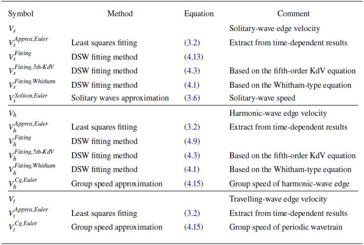
The solitary-wave edge velocity ( $V_s$ ), harmonic-wave edge velocity ( $V_h$ ) and travelling-wave edge velocity ( $V_t$ ) for different types of DSWs (with $\epsilon \bar {\eta }=0.05$ fixed). The meanings of the velocity symbols can be found in table 1.

Table 1.

Methods, equations and comments for different velocity symbols.

In the subsequent subsections, we will adopt multiple methods to investigate the edge velocities of DSWs. To clarify the definitions and prediction methods of these velocities, we present a symbol table (table 1) for convenient reference. The naming convention follows a specific rule: the subscript indicates the category of the edge, the first superscript denotes the method used to obtain this physical quantity, and the second superscript represents the equation upon which it is based.

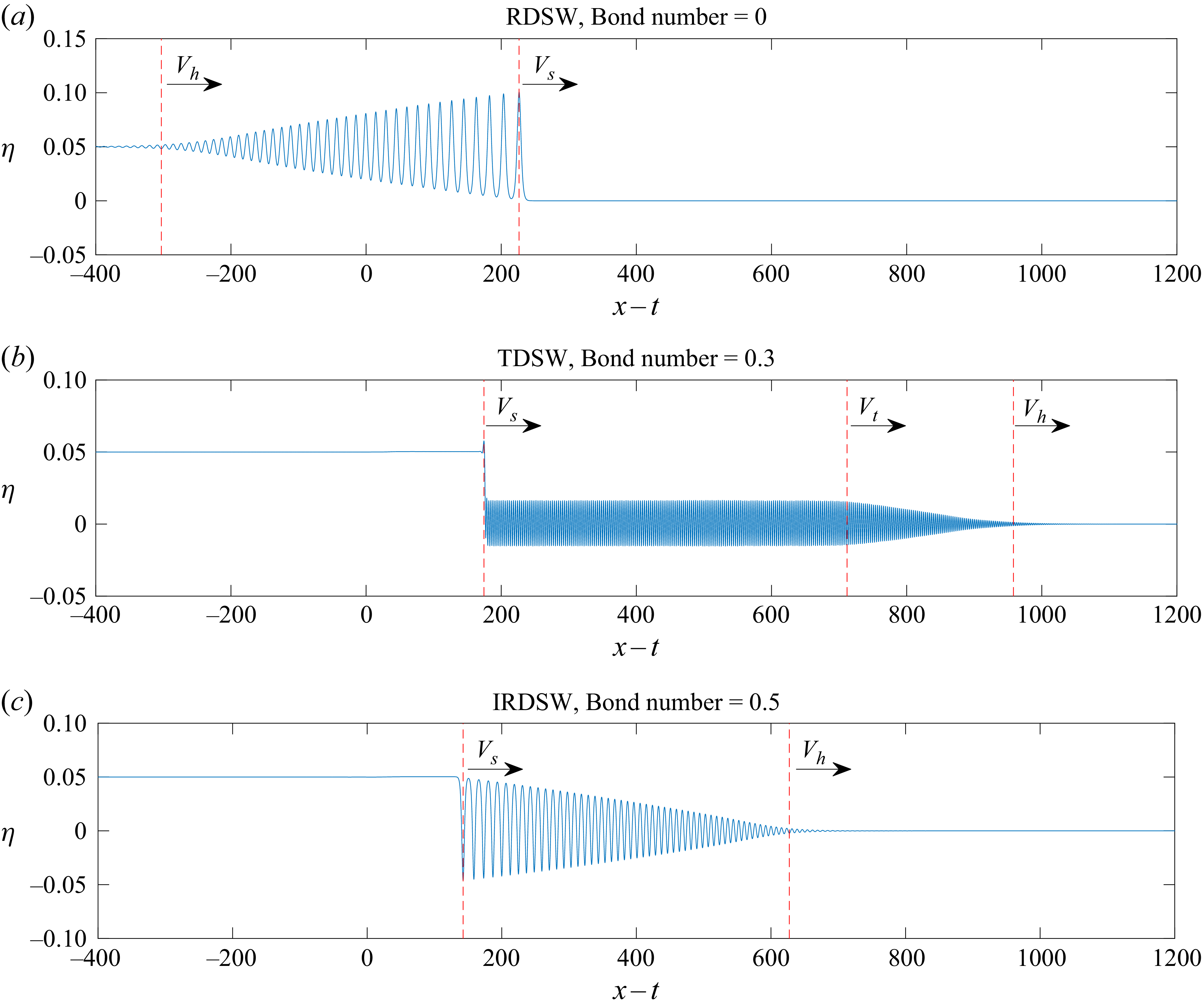
We begin by extracting the positions of solitary-wave and harmonic-wave edges from the numerical results, and the schematic diagram is shown in figure 4. In numerical terms, the harmonic-wave edge is defined as the location where the crest/trough amplitude reaches 5 % of the maximum amplitude in the horn-shaped wavepacket. In contrast, the solitary-wave edge can be identified differently depending on the case: it is represented by the leading wave crest in the RDSW case, the trailing wave crest in the TDSW case, or the trailing wave trough in the IRDSW case. Additionally, in the TDSW region, the travelling-wave edge marks the position where the crest/trough value in the horn-shaped region attains 95 % of the amplitude of the uniform wavetrain. Next, we apply the least squares method to fit the slope of the time–position curve and determine the numerical velocities of the solitary-wave edge ( $V_s^{\textit{Approx,Euler}}$ ), harmonic-wave edge ( $V_h^{\textit{Approx,Euler}}$ ) and travelling-wave edge ( $V_t^{\textit{Approx,Euler}}$ ). These velocities, derived by numerically solving the full Euler equations, are represented by circles, triangles and diamonds in figure 3. In the RDSW and IRDSW regions, $V_s^{\textit{Approx,Euler}}$ shows only slight variations with changes in the Bond number. However, in the RDSW region, as the Bond number increases, $V_h^{\textit{Approx,Euler}}$ approaches the Froude number $ \textit{Fr}=1$ , whereas $V_h^{\textit{Approx,Euler}}$ remains stable in the IRDSW region. In the TDSW region, $V_s^{\textit{Approx,Euler}}$ is greater than in the IRDSW region, while $V_h^{\textit{Approx,Euler}}$ experiences significant changes as the Bond number varies. The characteristic of the trailing edge disappears in the crossover region, therefore we do not present its edge velocity in figure 3.

Figure 4.

Schematic diagrams illustrating the edge velocities, including the solitary-wave edge velocity ( $V_s$ ), harmonic-wave edge velocity ( $V_h$ ) and travelling-wave edge velocity ( $V_t$ ): (a) RDSW with $V_s\gt V_h$ , (b) TDSW with $V_h\gt V_t\gt V_s$ , (c) IRDSW with $V_h\gt V_s$ . The red dashed lines are determined by the solitary-wave, travelling-wave and harmonic-wave edge locations calculated from the procedure outlined in § 4.2. The waveforms are derived from (3.2) using various Bond numbers.

El (Reference El2005) pointed out that the Whitham modulation equations become degenerate at the edges of DSWs in certain limiting cases. The edge velocity can be predicted using the nonlinear term and the dispersion relation of the system, without requiring a global integration of the modulation equations. This technique is known as the DSW fitting method, which we will use to predict the edge velocities in the subsequent analyses. Interested readers may refer to El & Hoefer (Reference El and Hoefer2016) and Sprenger & Hoefer (Reference Sprenger and Hoefer2017) for more details about the DSW fitting method. For this purpose, we focus on the Whitham equation, which is a fully dispersive and weakly nonlinear model originally proposed by Whitham to describe the wave breaking and peaking phenomena. According to Whitham (Reference Whitham1999), the nonlinear term $(3\sqrt {1+\eta }-2)\eta _x$ and the linear dispersion relation $\omega ^2=(1+B k^2)k\tanh (k)$ from (2.2) and (3.1) lead to the Whitham equation, which can be reformulated in the moving frame $x-t$ as

(4.1) \begin{align} \eta _t+3\left (\sqrt {1+\eta }-1\right )\eta _x+\int _{-\infty }^{\infty }K(x-\xi )\,\eta _\xi (\xi ,t)\,{\rm d}\xi =0, \end{align}

with the kernel

(4.2) \begin{align} K(x)=\frac {1}{2\pi }\int _{-\infty }^{\infty }\frac {\sqrt {(1+Bk^2)k\tanh (k)}-k}{k}\,{\rm e}^{{\mathrm i}kx}\,{\rm d}k. \end{align}

In the long-wave limit, (4.1) simplifies to the fifth-order KdV equation, which is a classical model used to describe gravity-capillary waves in shallow water:

(4.3) \begin{align} \eta _t+\frac {3}{2}\eta \eta _x+\frac {1}{6}\left (1-3B\right )\eta _{xxx}+\frac {1}{360}\big (19-30B-45B^2\big )\eta _{xxxxx}= 0. \end{align}

It is noted that considering the weakly nonlinear assumption, (4.1) can be rewritten in a more appealing form as

(4.4) \begin{align} \eta _t+\frac {3}{2}\eta \eta _x+\int _{-\infty }^{\infty }K(x-\xi )\,\eta _\xi (\xi ,t)\,{\rm d}\xi =0, \end{align}

commonly known as the Whitham equation, as referenced in Binswanger (Reference Binswanger2019). Thus to distinguish clearly, we refer to (4.1) as the Whitham-type equation. We apply the DSW fitting method to (4.1), offering a more precise dispersion relation than the fifth-order KdV model.

Following El (Reference El2005), we define the dispersion relation for (4.1) by introducing an infinitesimal perturbation around a mean level $\eta _0$ :

(4.5) \begin{align} \eta =\eta _0+\eta _1\,{\rm e}^{{\mathrm i}(k_hx-\omega _ht)},\quad \eta _1\ll \eta _0. \end{align}

Therefore, the leading-order dispersion relation of (4.1) can be recast to

(4.6) \begin{align} \omega _h(\eta _0,k_h)=N_h(\eta _0)\,k_h+f_h(k_h), \end{align}

with

(4.7) \begin{align} N_h(\eta _0)=3\big (\sqrt {1+\eta _0}-1\big ),\quad f_h(k_h)=\sqrt {\left (1+B k_h^2\right )k_h \tanh (k_h)}-k_h. \end{align}

If we assume that $k_h$ is a function related to the average height $\eta _0$ , and notice that the wavenumber $k_h$ vanishes at the solitary-wave edge, then we can determine the wavenumber by solving the ordinary differential equation (ODE)

(4.8) \begin{align} \frac {{\rm d}k_h}{{\rm d}\eta _0}=\frac {\partial \omega _h/\partial \eta _0}{N_h(\eta _0)-\partial \omega _h/\partial k_h},\quad k_h(\eta _s)=0,\ \eta _0=\eta _s, \end{align}

where the average level of the solitary-wave edge is represented by $\eta _s$ . Additionally, $V_h$ can be determined using the dispersion relation (4.6), which is associated with the wavenumber at the harmonic-wave edge, denoted as

(4.9) \begin{align} V_h^{\textit{Fitting}}=\frac {\partial \omega _h(\eta _0,k_h)}{\partial k_h},\quad k_h=k_h(\eta _h),\quad \eta _0=\eta _h, \end{align}

where $\eta _h$ stands for the average height of the harmonic-wave edge.

On the other hand, the velocity of the solitary-wave edge necessitates an analogy to the dispersion relation that applies to periodic waves. El (Reference El2005) demonstrates that this can be derived from

(4.10) \begin{align} \omega _s(\eta _0,k_s)=-\mathrm{i} \omega _h(\eta _0,\mathrm{i} k_s)=N_s(\eta _0)\,k_s+f_s(k_s), \end{align}

with

(4.11) \begin{align} N_s(\eta _0)=3\big (\sqrt {1+\eta _0}-1\big ),\quad f_s(k_s)=\sqrt {(1-B k_s^2)k_s\tan (k_s)}-k_s. \end{align}

In the same way, we assume that $k_s$ is a function related to the average height $\eta _0$ , and apply the condition that $k_s$ equals zero at the harmonic-wave edge. Consequently, the ODE that we need to solve can be expressed as

(4.12) \begin{align} \frac {{\rm d}k_s}{{\rm d}\eta _0}=\frac {\partial \omega _s/\partial \eta _0}{N_s(\eta _0)-\partial \omega _s/\partial k_s},\quad k_s(\eta _h)=0,\ \eta _0=\eta _h. \end{align}

The solitary-wave edge velocity can be inferred from the special situation of (4.10), given by

(4.13) \begin{align} V_s^{\textit{Fitting}}=\frac {\omega _s(\eta _0,k_s)}{k_s},\quad k_s=k_s(\eta _s),\ \eta _0=\eta _s. \end{align}

For the RDSW case, we set $\eta _h=\epsilon \bar {\eta }$ and $\eta _s=0$ . In contrast, for the IRDSW case, $\eta _h=0$ and $\eta _s=\epsilon \bar {\eta }$ are established based on figure 1. Finally, we recover the velocity in the original frame by adding the reference speed $ \textit{Fr}=1$ .

The DSW fitting method can also be applied to the fifth-order KdV equation (4.3) and the Whitham equation (4.4) using a similar procedure, and interested readers are referred to Sprenger & Hoefer (Reference Sprenger and Hoefer2017) and Binswanger (Reference Binswanger2019) for more details. In numerical simulations, we first solve the ODEs (4.8)–(4.13) within the framework of the fifth-order KdV equation to determine the wavenumbers at both the solitary-wave and harmonic-wave edges. These results provide initial estimates for the Newton–Raphson method, which is employed to find the roots of the ODEs (4.8) and (4.12) in the context of the Whitham-type equation (4.1). Ultimately, the velocity predictions of the DSW edges are deduced from (4.9) and (4.13).

Figure 3 demonstrates that the DSW fitting method effectively predicts the edge velocities in both the RDSW and IRDSW regions. The velocity of the solitary-wave edge ( $V_s^{\textit{Fitting}}$ ) changes slightly, while the harmonic-wave edge velocity ( $V_h^{\textit{Fitting}}$ ) approaches $ \textit{Fr}=1$ in the RDSW region, and remains consistent in the IRDSW region. The fifth-order KdV equation (4.3) and the Whitham-type equation (4.1) produce similar results for predicting $V_s^{\textit{Approx,Euler}}$ . While the fifth-order KdV equation fails to predict $V_h^{\textit{Approx,Euler}}$ accurately, the Whitham-type equation provides a more reliable estimate. However, the DSW fitting method encounters difficulties in the TDSW region. For the variable $V_s^{\textit{Fitting}}$ , within the framework of the fifth-order KdV equation (4.3), the predicted wavenumbers of the solitary-wave edge, as described by (4.13), become complex numbers when the Bond number is less than 0.380. Additionally, for the Whitham-type equation (4.1), the Newton–Raphson method fails to converge when the Bond number is below 0.398. The values of $B$ predicted by the fifth-order KdV equation ( $B=0.380$ ) and the Whitham-type equation ( $B=0.398$ ) provide estimates for the critical threshold for the transition from TDSW to IRDSW. This transition corresponds to the critical value of $B=0.41$ in the full Euler equations, as illustrated in figure 3. In regard to $V_h^{\textit{Fitting}}$ , although both simplified equations can indicate the general trend of $V_h^{\textit{Approx,Euler}}$ , the error increases as the Bond number approaches the crossover region. The limitations of theoretical predictions in the TDSW region are attributed to the special structure of this type of solution: the ODE system (4.8)–(4.13) depicts the continuous change in wavenumber, yet there exists a shock connecting the solitary edge and the periodic wavetrain, which creates a discrepancy that the DSW fitting method is unable to address.

In contrast to the RDSW or IRDSW region, the edge velocities in the TDSW region exhibit distinct characteristics: (i) the velocity of the harmonic-wave edge significantly decreases from $V_h^{\textit{Approx,Euler}}=1.224$ to $1.137$ as the Bond number increases; (ii) the velocity of the solitary-wave edge is greater than that observed in the IRDSW region. These differences require an explanation that goes beyond the classical DSW theory, which we will address in future investigations. In § 4.3, we will present the velocity prediction for the TDSW region, and in § 4.4, we will present the prediction of the TDSW envelope.

4.3. The analogy between solitary waves and DSWs

The analogy between solitary waves and DSWs elucidates their distinct yet interconnected dynamics. Solitary waves are permanent, isolated waveforms that retain their shape due to a balance between nonlinearity and dispersion, allowing them to travel at a constant speed. In contrast, DSWs arise from resolving an initial discontinuity in a medium and are characterised by a rapidly oscillating series of waveforms that bridge two distinct states. The analogy between solitary waves and DSWs, which we will discuss below, underscores the relationship between the fields of travelling waves and transient waves.

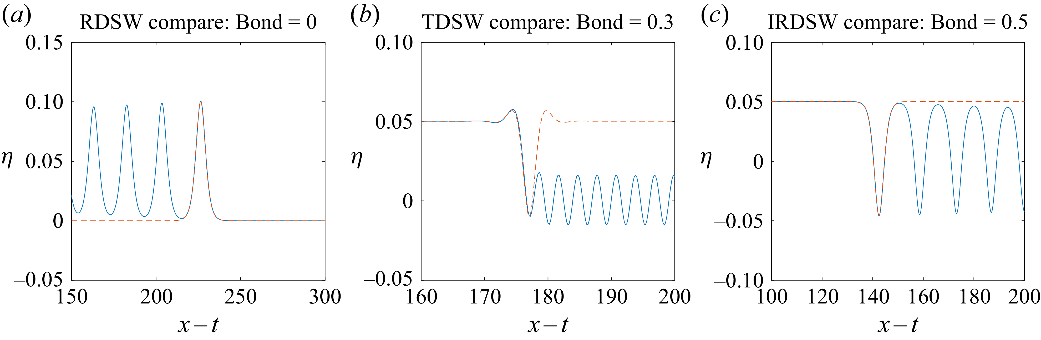
The structures of RDSWs and IRDSWs demonstrate the transition from solitary waves to periodic waves. Figures 5(a) and 5(c) emphasise the resemblance between the solitary-wave edges of DSWs and solitary waves, as illustrated in figures 1(a) and 1(g). In contrast, the TDSW structure exhibits a distinct pattern: it starts as a solitary wave, then evolves into a uniform periodic wavetrain, and ultimately the amplitude of the periodic wave decreases to zero, forming a horn-shaped wavepacket. This observed pattern suggests the need for further exploration into the mechanisms behind the generation and evolution of TDSWs.

Figure 5.

Comparisons of various DSWs with solitary waves ( $\epsilon \bar {\eta }=0.05$ ) for different Bond numbers: (a) $B=0$ , (b) $B=0.3$ , and (c) $B=0.5$ . The blue solid lines indicate DSWs predicted by (3.2), while the red dashed lines denote solitary waves obtained from (3.6).

Next, we explore the analogy between solitary waves with oscillatory pulses and TDSWs, aiming to generalise conclusions drawn from RDSWs and IRDSWs to the realm of TDSWs. First, in this paper, we define a ‘solitary wave with an oscillatory pulse’ as a solitary wave that incorporates a periodic wavetrain within its pulse, without displaying significant oscillations in the tails. The gravity-capillary solitary waves with oscillatory pulses were initially computed by Dias (Reference Dias1994) within the framework of the Euler equations, specifically examining structures that include two, three and five pendant-shaped bubbles. In Dias & Vanden-Broeck (Reference Dias and Vanden-Broeck1996), solutions with two troughs are illustrated in figures 4.3(a) and 4.3(b), corresponding to $B=0.2444$ and $B=0.3747$ , respectively. Additionally, solutions with three troughs are presented in figures 4.5(a) and 4.5(b), with $B=0.2769$ and $B=0.3665$ , respectively. As the Bond number approaches $1/3$ , the fifth-order KdV equation has been confirmed to approximate the full Euler system effectively. The relationship between this type of solitary wave in the Euler equations and the fifth-order KdV model was demonstrated by Dias & Vanden-Broeck (Reference Dias and Vanden-Broeck1996). They also showed that there are an infinite number of homoclinic orbits in the reduced model. In the field of dynamical systems, a homoclinic orbit is defined as a trajectory in phase space that connects a saddle equilibrium point back to itself. Specifically, within the fifth-order KdV model, a homoclinic orbit represents a form of solitary wave. As a result, the presence of an infinite number of homoclinic orbits suggests that an infinite variety of solitary waves can be anticipated in this model. Sprenger & Hoefer (Reference Sprenger and Hoefer2020) calculated solitary waves with oscillatory pulses in the fifth-order KdV equation, and superimposed these travelling waves on the TDSW structure, emphasising the link between steady and unsteady solutions. Our subsequent calculations will extend the above conclusions to the full Euler equations, shedding light on the relationship between solitary waves with oscillatory pulses and TDSWs.

To achieve this goal, the first step is to rescale the full Euler equations (refer to (2.2) and (3.1)). This rescaling is necessary because the amplitude of the solitary wave decreases to a value of $\epsilon \bar {\eta }$ , rather than to zero, at the edge of the TDSW. We define the scales for length, time and potential as

(4.14) \begin{align} h_0(1+\epsilon \bar {\eta }),\quad \sqrt {\frac {h_0(1+\epsilon \bar {\eta })}{g}},\quad \sqrt {g h_0^3\left (1+\epsilon \bar {\eta }\right )^3}, \end{align}

respectively, and set the corresponding Bond number as $\widetilde {B}= {B}/{(1+\epsilon \bar {\eta })^2}$ . Consequently, we normalise the mean height to $h_0=1$ , and ensure that the amplitude of the solitary wave with an oscillatory pulse matches that of the TDSW at infinity for comparison purposes.

We present a comparison of the TDSW illustrated in figure 1(e) with solitary waves that contain between two and nine troughs, as shown in figure 6. From this comparison, we deduce that the number of periodic oscillations in the central part may increase indefinitely to align with the solitary-wave edge of the TDSW. Additionally, figure 7 displays a comparison of TDSWs across a Bond number range from 0.29 to 0.40, alongside solitary waves featuring five troughs in the pulse. This suggests that solitary waves with oscillatory pulses can occur across a wide range of Bond numbers. As the Bond number increases, the amplitude of the uniform wavetrain progressively rises, peaking at $\eta =0.05$ , while the wavelength becomes longer. At the same time, the solitary-wave edge of the TDSW closely resembles that of the IRDSW, reflecting a gradual transition from TDSW to IRDSW.

Figure 6.

(a–h) Comparisons between the TDSW ( $\epsilon \bar {\eta }=0.05$ and $B=0.3$ ) and solitary waves that have oscillatory pulses with varying numbers of oscillations. The blue solid lines represent the TDSW at $t=5000$ predicted by (3.2), while the red dashed lines depict the solitary waves with oscillatory pulses derived from (3.6), showcasing troughs ranging from two to nine.

Figure 7.

The TDSWs with various Bond numbers ( $\epsilon \bar {\eta }=0.05$ ) compared to solitary waves with oscillatory pulses. (a–l) The comparisons between solitary waves featuring five troughs and TDSWs with Bond numbers ranging from 0.29 to 0.40. The blue solid lines represent TDSWs at $t=5000$ predicted by (3.2), while the red dashed lines depict solitary waves with five troughs derived from (3.6).

To further explore the relationship between TDSWs and solitary waves with oscillatory pulses, it is essential to compare their velocities. It is found that the DSW fitting method does not accurately predict the solitary-wave edge velocity in the TDSW region. To address this issue, we derive the velocity directly from numerical solutions of solitary waves with five troughs in pulse. The calculations for travelling-wave solutions assume a still-water condition; therefore, we reintegrate the reference velocity into the analysis, applying a shallow-water assumption with $\phi _x=\epsilon \bar {\eta }=0.05$ . The results presented in figure 8(a) demonstrate a satisfactory fit, indicating that the solitary-wave edge velocity of the TDSW coincides with the propagation speed of a solitary wave featuring an oscillatory pulse.

Figure 8.

Predictions of edge velocities for TDSWs with $\epsilon \bar {\eta }=0.05$ : (a) $V_s^{\textit{Approx,Euler}}$ (circles) and the solitary wave speed $V_s^{\textit{Soliton,Euler}}$ (triangles); (b) $V_t^{\textit{Approx,Euler}}$ (circles) and the group velocity of the periodic wavetrain $V_t^{\textit{Cg,Euler}}$ (triangles); and (c) $V_h^{\textit{Approx,Euler}}$ (circles), $V_h^{\textit{Fitting,Whitham}}$ (solid line), and the group velocity $V_h^{\textit{Cg,Euler}}$ (squares). (d) A time-dependent progression of TDSW with $B=0.32$ , obtained from (3.2). For definitions of the velocity symbols, please refer to table 1.

In figure 8(b), the travelling-wave edge velocity is predicted based on the group velocity of the periodic wavetrain appearing in the pulse, denoted as $V_t^{\textit{Cg,Euler}}$ . The dimensionless group velocity is expressed as follows:

(4.15) \begin{align} C_g = \frac {\left (k + B k^3\right ) \text{sech}^2(k)+\left (1 + 3 B k^2\right ) \tanh (k)}{2 \sqrt {k \left (1 + B k^2\right ) \tanh (k)}}, \end{align}

where $k$ is extracted from the periodic wavetrain. Although the predicted velocity is slightly higher than the actual velocity, it effectively captures the trend of velocity variation in response to changes in the Bond number. According to Whitham (Reference Whitham1999), in a non-uniform wavetrain, different wavenumbers propagate with their respective group velocities. On the left-hand side of the travelling-wave edge, the wavenumber remains constant, while on the right-hand side, it increases continuously. When one moves with the group velocity at the travelling-wave edge, the same local wavenumber and frequency can be observed. Meanwhile, the wave crests continue to pass, suggesting that the region of the uniform periodic wavetrain is expanding. This may provide an understanding that $V_t^{\textit{Approx,Euler}}$ is approximately equal to the local group velocity $V_t^{\textit{Cg,Euler}}$ .

In figure 8(c), the velocity of the harmonic-wave edge is analysed using the DSW fitting method applied to (4.1), although the validity of this method was not thoroughly examined in the TDSW region. The prediction becomes less accurate near the crossover region (as $B\rightarrow 0.29$ ). Nevertheless, as the Bond number increases, the prediction generally provides a reasonable approximation, particularly as the solution gradually transitions from TDSW to IRDSW. Additionally, we extract the wavenumber at the harmonic-wave edge and calculate the corresponding group velocity, $V_h^{\textit{Cg,Euler}}$ , according to (4.15), which closely matches $V_h^{\textit{Approx,Euler}}$ .

The analyses and comparisons indicate that the high platform and its extended uniform wavetrain within the TDSW represent a part of a solitary wave characterised by an oscillatory pulse. In other words, the TDSW illustrates the modulation process that transitions from a solitary wave with an oscillatory pulse to smaller periodic waves through a horn-shaped wavepacket that gradually lengthens over time. In this regard, the observed patterns are fundamentally similar to those found in the RDSW and IRDSW regions.

4.4. Modulation parameters in TDSWs

Recall that the Whitham modulation equations (2.7) and (2.16) are essentially derived using the Stokes expansion. Considering the variety of periodic waves present in the TDSW structure, this approach aids in predicting the modulation parameters in the TDSW process. These parameters include the wavenumber $k$ , the amplitude of the periodic wave $a$ , and the wave mean $b$ .

It is noted that the rescaled modulation equations can be obtained by simply setting $h_0=g=1$ and replacing $\tau$ with $B$ . By utilising the shallow-water assumption, where $\phi _x=\eta$ , we establish a relationship between the mean flow and the wave mean, given by $b=\beta$ . The remaining parameters in this problem are $a$ , $k$ and $b$ . The first equations in (2.7) and (2.16) describe the modulation of the wavenumber $k$ and the amplitude $a$ . On the other hand, the changes in the wave mean $b$ can be explained by the second equations in (2.7) and (2.16), which are identical when considering the higher-order terms in the modulation. We combine the second equations in (2.7) and (2.16) into a single equation by applying appropriate weights in our numerical simulations. This operation aims to maintain the average value of the wave mean $b$ at the desired level. It should be noted that relying solely on either the second equation in (2.7) or the second equation in (2.16) would result in a discontinuity at $x=0$ , leading to incorrect results. To facilitate comparison, we present our findings in the moving reference frame $x-t$ . Thus the governing modulation equations can be rewritten as

(4.16) \begin{align} \begin{aligned} &\frac {\partial }{\partial t}\left (\frac {E}{\omega _0}\right )+\frac {\partial }{\partial x}\left [(c_g-1)\frac {E}{\omega _0}\right ]=0,\\&\frac {\partial k}{\partial t}+\frac {\partial (\omega -k) }{\partial x}=0,\\ &\frac {\partial b}{\partial t}+\frac {1}{\alpha _1+\alpha _2}\frac {\partial }{\partial x}\left [\alpha _1bh+\alpha _1\frac {E}{c_p}+\alpha _2\gamma -(\alpha _1+\alpha _2)b\right ]=0, \end{aligned} \end{align}

where $\alpha _1$ and $\alpha _2$ are the weights to be determined later. We extract the values of $a$ , $k$ and $b$ from the TDSW numerical results, using parameters $\epsilon =0.05$ , $B=0.32$ and $t=5000$ . We establish the initial condition for (4.16) as follows:

(4.17) \begin{align} (a,k,b)(x,t=0) = \begin{cases} (a_l,k_l,b_l), & x\lt 0,\\ (0,k_r,0), & x\geqslant 0, \end{cases} \end{align}

where $a_l$ , $k_l$ and $b_l$ represent the mean values of the corresponding parameters within the region $x\in (220,320)$ in the simulation at $t=5000$ , and $k_r$ denotes the maximum value of the wavenumber extracted from the TDSW numerical result. We employ an algorithm inspired by the Roe scheme to numerically solve (4.16) with the initial condition (4.17):

(4.18) \begin{align} \begin{aligned} &u_j^{n+1}=u_j^{n}-\frac {\Delta t}{\Delta x}\left (\hat {f}_{j+\frac {1}{2}}^n-\hat {f}_{j-\frac {1}{2}}^n\right )\!,\\&\hat {f}_{j+\frac {1}{2}}^n= \begin{cases} f(a_j,k_j,b_j),&\theta _{j+\frac {1}{2}}\geqslant 0,\\ f(a_{j+1},k_{j+1},b_{j+1}),&\theta _{j+\frac {1}{2}}\lt 0, \end{cases}\\ &\theta _{j+\frac {1}{2}}=\frac {f(a_{j+1},k_{j+1},b_{j+1})-f(a_j,k_j,b_j)}{u(a_{j+1},k_{j+1},b_{j+1})-u(a_j,k_j,b_j)}\!, \end{aligned} \end{align}

where $u$ represents the parameters $E/\omega _0$ , $k$ and $b$ , while $f$ denotes the corresponding fluxes. The notation $j$ refers to the value at the discrete point $x_j$ , and $n$ indicates the $n$ th time step. This scheme effectively eliminates most of the non-physical oscillations caused by the discontinuous initial data. In our simulations, we set $\alpha _1=3$ and $\alpha _2=8$ in (4.16), and present the results for the amplitude squared $a^2$ , which is proportional to the energy $E$ .

The comparison between the solutions to the modulation (4.16) and the parameters derived from the full Euler simulations using smoothed step initial data is presented in figure 9(a–c), demonstrating excellent agreement. High-order modulation theory is essential when considering small oscillations in wave parameters and minor discrepancies between the modulation solutions and the full Euler results; however, this topic is beyond the scope of this discussion. As we derive predictions for the key wave parameters ( $a$ , $k$ and $b$ ), we can also forecast wavepacket behaviour in the TDSW region using $a+b$ and $-a+b$ , as illustrated in figure 9(d). The results indicate a remarkable alignment, suggesting that TDSWs may be viewed as the modulation process of periodic wavetrains in these cases.

Figure 9.

Numerical results for the TDSW compared with the predictions from the Whitham modulation equations under the conditions $\epsilon \eta =0.05$ , $B=0.32$ and $t=5000$ . The comparison includes: (a) amplitude squared $a^2$ , (b) wavenumber $k$ , (c) wave mean $b$ , and (d) wavepacket as predicted by the Whitham theory and observed in the TDSW simulation. The blue circles/line represent the results from the TDSW simulation using (3.2), while the red solid lines correspond to the Whitham modulation theory for (4.16).