


1 INTRODUCTION
Consider a setup in which a decision maker (DM) has to decide whether or not to assign a treatment after observing data with observations from the untreated and treated populations.Footnote 1 The DM could be a policymaker who applies a treatment to the entire population or a person who is applying the treatment to an individual (e.g., herself). As examples of the latter setup, think of an individual who chooses between two hotels on an internet platform after observing a certain number of ratings or a medical doctor who considers a treatment for a patient after observing a certain number of outcomes from treated and untreated patients.
This article adds to a short but growing literature on finding treatment rules that have finite-sample optimality properties. In most of the literature, the focus is on the expected outcome under the chosen treatment rule.Footnote
2
Given that typically there is no treatment rule that is uniformly best over all possible joint distributions for
$(Y_{0},Y_{1}),$
 where
$Y_{0}$
 and
$Y_{1}$
 denote random variables for outcomes without and with treatment, respectively, one has to resort to other criteria for optimality. One option is to consider a prior over the space of joint distributions and maximize expected outcome for this particular prior. Another option is to focus on admissible treatment rules, but that criterion typically does not single out an individual treatment rule (see Manski and Tetenov, Reference Manski and Tetenov2023; Montiel Olea et al., Reference Montiel Olea, Qiu and Stoye2026). Alternatively, one might consider finding a treatment rule that maximizes minimal expected outcome where the minimum is taken over all joint distributions of
$(Y_{0},Y_{1}).$
 However, if there exists a distribution that assigns the minimal possible values in the shared domains of
$Y_{0}$
 and
$Y_{1}$
 with probability one, then any treatment rule is going to be optimal according to this criterion and therefore also the “max–min” approach is not pinning down a unique rule. For that reason, instead, the so-called “minimax regret” criterion is often adopted that determines treatment rules that minimize the maximal regret where regret is defined as the difference between the largest expected outcome that could be achieved for any treatment rule and the expected outcome under the treatment rule under consideration, and the maximum is taken with respect to all possible distributions for
$(Y_{0},Y_{1}).$
 Stoye (Reference Stoye2009) derives minimax regret rules in finite samples for the case of two treatments under various sampling schemes, namely, matched pairs, random sampling, and testing an innovation, and furthermore provides near-uniqueness results.
In this project, we are interested in a setup where, rather than expected outcome, the DM is concerned about the
$\alpha $
 -quantile of the outcome (for a given
${\alpha \in \lbrack 0,1]}$
 ). Wang et al. (Reference Wang, Zhou, Song and Sherwood2018) consider robust estimation of the quantile-optimal treatment regime and provide arguments as to why focusing on a quantile rather than the mean may be sensible in certain applications. In fact, in many applications, the tail of the outcome distribution is at the center of interest. For example, when evaluating job training programs to improve earnings, the focus is often on earnings in the lower tail, and likewise in survival analysis (e.g., survival time of cancer patients), the lower tail is of key importance. Wang et al. (Reference Wang, Zhou, Song and Sherwood2018, Sect. 2) provide numerical evidence where the mean-optimal treatment is detrimental for patients in the lower tail. In Economics, one might be interested in median income (case
$\alpha =1/2)$
 or a minimal level of educational achievement for schoolchildren, “no child left behind” (case
$\alpha =0$
 ). See Manski (Reference Manski1988) who studies the “quantile utility” model whose predictions, unlike the expected utility model, are invariant under ordinal transformations of utility. Subsequently, Rostek (Reference Rostek2010) axiomatizes quantile preference and, recently, Manski and Tetenov (Reference Manski and Tetenov2023) suggest considering various deviations from mean loss including quantiles. Also, see Chambers (Reference Chambers2009).Footnote
3
As the main contribution of this article, we derive minimax regret treatment rules
$\delta $
 in finite samples when an
$\alpha $
 -quantile of the outcome distribution is the focus of interest and outcomes
$Y_{0}$
 and
$Y_{1}$
 take values in the unit interval. That is, the objective function for the DM is
$q_{s,\alpha }(Y_{B(\delta (w_{N}))}),$
 where
$Y_{B(\delta (w_{N}))}$
 denotes random outcomes generated when the treatment rule
$\delta $
 is used, with
$B$
 representing a Bernoulli random variable that equals
$1$
 with probability
$\delta (w_{N}),$
 and
$q_{s,\alpha }(Y_{B(\delta (w_{N}))})$
 denotes the
$\alpha $
 -quantile of
$Y_{B(\delta (w_{N}))}$
 when the joint distribution of
$(Y_{0},Y_{1})$
 equals
$s$
 .
Somewhat surprisingly, we show that under various sampling schemes all treatment rules are minimax regret, namely, in case i), when the sample consists of a fixed number of treated and a fixed number of untreated units (i.e., unbalanced panels are allowed for) and in case ii), under random assignment with arbitrary treatment assignment probability in the sample equal to
$p\in (0,1).$
 In both cases i) and ii), maximal regret equals 1 for any treatment rule.
On the other hand, in case iii), “testing an innovation,” that is, the case where only data on
$Y_{1}$
 is observed and the
$\alpha $
 -quantile
$q_{s,\alpha }(Y_{0})$
 of
$Y_{0}$
 is known, where again the subscript
$s$
 denotes the joint distribution of
$(Y_{0} ,Y_{1})$
 , if
$q_{s,\alpha }(Y_{0})>1/2,$
 then
$\delta \equiv 0$
 is the unique minimax rule, if
$q_{s,\alpha }(Y_{0})<1/2,$
 then
$\delta \equiv 1$
 is a minimax rule, and finally, if
$q_{s,\alpha }(Y_{0})=1/2,$
 then any treatment rule
$\delta $
 is minimax regret; in each case, for minimax treatment rules
$\delta $
 , we obtain the formula
$\min \{q_{s,\alpha }(Y_{0}),1-q_{s,\alpha }(Y_{0})\}$
 for the maximal regret.
Obviously, like for the case where expected outcomes are the focus, also here the max–min criterion is not informative. Namely, as long as the joint distribution of
$(Y_{0},Y_{1})$
 can be chosen such that
$q_{s,\alpha } (Y_{0})=q_{s,\alpha }(Y_{1})=0,$
 that is, the worst possible outcome under the given restriction that
$Y_{0},Y_{1}\in \lbrack 0,1],$
 any treatment rule would be max–min optimal. In contrast though, to the case where expected outcomes are the focus, for quantiles also minimax regret is not informative for sampling designs i) and ii) and also for iii) when
$q_{s,\alpha }(Y_{0})=1/2.$

The typical strategy in the extant literature for determining minimax regret rules when the focus is on expected outcomes is via a Nash equilibrium approach in a fictitious zero sum game in which the DM plays against an antagonistic nature whose payoff equals regret. To establish that a particular treatment rule
$\delta $
 is minimax regret, one attempts to guess a “state of nature”
$s$
 , allowed to be mixed strategy (over a finite number of states), called a least favorable distribution, for which the pair
$(\delta ,s)$
 constitutes a Nash equilibrium. Existence of such a pair
$(\delta ,s)$
 implies that
$\delta $
 is indeed a minimax regret rule (see, e.g., Berger, Reference Berger1985; Stoye, Reference Stoye2009; Chen and Guggenberger, Reference Chen and Guggenberger2026). Often, in a first step, one restricts outcomes to be Bernoulli and finds a minimax rule in this simplified setup and then, in a second step, uses the so-called coarsening approach to tackle the general case (see, e.g., Cucconi, Reference Cucconi1968; Gupta and Hande, Reference Gupta, Hande and Saleh1992; Schlag, Reference Schlag2003, Reference Schlag2006). When nature picks a state of the world trying to inflict high regret, it faces the trade-off that, on the one hand, a high differential between expected outcomes with and without treatment is needed, but, on the other hand, the more different the distributions of
$Y_{0}$
 and
$Y_{1}$
 are the easier the DM can tell them apart using the sample information.
The proof structure for the main results in this article differs from the one just described. Namely, for cases i) and ii), we show that for any treatment rule
$\delta ,$
 one can find a state of nature
$s=s_{\delta }$
 such that
$s$
 inflicts the highest possible regret, namely, 1. That insight is sufficient to establish that all rules are minimax regret and that maximal regret equals 1 for all treatment rules. It is noteworthy and remarkable that, despite the trade-off just described, nature is powerful enough to inflict maximal regret on the DM. Even more surprisingly, the conclusions under i) and ii) continue to be true even if nature is restricted to only Bernoulli distributions. The proof for part iii) relies on the main insight that if
$\delta \neq 0,$
 then there exists a state of nature such that regret equals the known
$\alpha $
 -quantile of
$Y_{0}.$
 For that to be true, it is sufficient for nature to have discrete distributions, supported on
$N+1$
 points, at its disposal.
We start off with the case with no covariates and then allow for a discrete-valued covariate in the model. In the latter case, a treatment rule maps a sample onto treatment probabilities for each of the
$K$
 possible outcomes of the covariate. Not surprisingly, given the results without a covariate, we find that in cases i) and ii), and case iii) with known quantile equal to 1/2, again, each treatment rule is minimax regret, while in case iii) when the known quantile is different from 1/2, no-data rules are minimax regret.
We include a small finite sample simulation study in the case of “testing an innovation” where we simulate regret of various treatment rules, namely, the empirical success rule and several no-data rules. The study corroborates our theoretical findings about minimax regret treatment rules and the formulas for maximal regret that we derive.
The remainder of the article is organized as follows. Section 2 introduces the theoretical setup for our notion of a minimax regret rule with quantiles and contains analytical results when no covariates are included. In Section 2.1, we present various approaches for how quantiles could be incorporated into the Waldean framework of statistical decision theory and juxtapose them with our approach. Section 2.2 derives minimax regret treatment rules under various sampling schemes and also provides a brief discussion of minimax regret treatment rules when certain restrictions are imposed on the states of nature. Section 2.3 simulates the performance of various treatment rules in finite samples in the case of testing an innovation. Finally, Section 3 derives minimax regret treatment rules in the case where covariates are included in the model. All proofs are given in the Appendix.
2 THEORETICAL SETUP WITHOUT COVARIATES
A DM has to decide whether or not to assign treatment after being informed about the population by a finite sample. The setup is very similar to the one in Stoye (Reference Stoye2009) with one key modification. Namely, rather than focusing on mean outcomes, here we are concerned with the
$\alpha $
 -quantile of the outcome distribution.
For most parts of the article, potential outcomes
$Y_{0}$
 and
$Y_{1}$
 for untreated/treated individuals are restricted to the unit interval

where
$S$
 is assumed known to the DM. At first, different members of the population are all identical to the DM. Later, we will consider the case where a covariate is included and treatment assignment can be made conditional on the realization of the covariate.
By
$\mathbb {S}$
 , we denote the set of “states of the world”
$s$
 , where an
$s$
 denotes a possible joint probability distribution over the potential outcomes for
$Y_{0}$
 and
$Y_{1}.$
 Unless otherwise stated,
$\mathbb {S}$
 is unrestricted and contains all possible joint distributions for
$Y_{0}$
 and
$Y_{1}$
 on
$S^{2}.$
 Upon observing a sample
$w_{N}=(t,y)$
 of size
$N$
 of treatment statuses
$t=(t_{1},\ldots ,t_{N})$
 and outcomes
$y=(y_{1},\ldots ,y_{N})$
 , where the
$i$
 -th component of
$y,\, y_{i},$
 is an independent realization of
$Y_{t_{i}}$
 and
$t_{i}$
 denotes the treatment received by individual
$i,$
 the task for the DM is to choose

which denotes the probability with which treatment is assigned.Footnote
4
Namely, which treatment the DM assigns is determined as an independent draw of the Bernoulli random variable
$B=B(\delta (w_{N}))\in \{0,1\}$
 that equals
$1$
 with probability
$\delta (w_{N})$
 and is assumed to be independent of all other random objects. Therefore, the setup here allows for randomized treatment rules.
Let
$\alpha \in \lbrack 0,1].$
 Given a state of the world
$s$
 and a statistical treatment rule
$\delta ,$
 the objective function for the DM is

where
$Y_{B(\delta (w_{N}))}$
 denotes random outcomes generated when the treatment rule
$\delta $
 is used, and
$q_{s,\alpha }(Y_{B(\delta (w_{N}))})$
 denotes the
$\alpha $
 -quantile of
$Y_{B(\delta (w_{N}))}$
 when the state of the world is
$s\in \mathbb {S}.$
 In particular, when the treatment rule
$\delta (w_{N})$
 equals 0 (or 1), then with probability 1
$Y_{B(\delta (w_{N}))}$
 equals
$Y_{0}$
 (or
$Y_{1}$
 ).
By definition, an
$\alpha $
 -quantile of a scalar-valued random variable
$X$
 with domain
$D$
 is any number
$q\in D$
 that satisfies

Clearly then, any
$\alpha $
 -quantile of
$Y_{0},\, Y_{1}$
 , and
$Y_{B(\delta (w_{N}))}$
 is an element of [0,1]. In general, this definition does not lead to a unique
$\alpha $
 -quantile. The definition allows for the case where a quantile has a nonzero point mass. To be explicit in cases where there is non-uniqueness, we make the following definition that hinges on a choice
$r\in \lbrack 0,1].$

Definition (
$\alpha $
 -quantile): Let
$Q$
 denote the set of all
$\alpha $
 -quantiles
$q$
 . For
$\alpha \in (0,1)$
 , we define the
$\alpha $
 -quantile as

When
$\alpha =0$
 , we use
$\sup Q$
 (i.e., we use
$r=1$
 ) and when
$\alpha =1$
 , we use
$\inf Q$
 (i.e., we use
$r=0). $

From now on, by
$q_{s,\alpha }(Y_{B(\delta (w_{N}))})$
 , we denote the
$\alpha $
 -quantile of
$Y_{B(\delta (w_{N}))}$
 when the state of the world is
$s.$
 For simplicity of notation, unless needed for clarity, we do not index that expression by
$r.$

By definition, regret of the treatment rule
$\delta $
 for a given distribution
$s$
 of
$(Y_{0},Y_{1})$
 equals

where
$\mathbb {D}$
 denotes the set of all possible treatment rules. In words, regret equals the difference between the highest
$\alpha $
 -quantile that could have been achieved for any treatment rule
$d\in \mathbb {D}$
 and the
$\alpha $
 -quantile obtained for the particular treatment rule
$\delta $
 for the given state of nature
$s.$
 If
$q_{s,\alpha }(Y_{1})\geq q_{s,\alpha }(Y_{0})$
 (
$q_{s,\alpha }(Y_{1})<q_{s,\alpha }(Y_{0}))$
 and
$d^{\ast }=1$
 (
$d^{\ast }=0$
 ) is an element of
$\mathbb {D,}$
 then
$\sup _{d\in \mathbb {D}}u(d,s)$
 is taken on by
$d^{\ast }$
 and equals
$q_{s,\alpha }(Y_{1})$
 (
$q_{s,\alpha }(Y_{0})$
 ) (see Lemma 3(ii) in the Appendix). If restrictions are imposed on
$\mathbb {D,}$
 then
$\sup _{d\in \mathbb {D}}u(d,s)$
 may not be taken on by any element in
$\mathbb {D}\mathfrak {.}$
 Again, without restrictions,
$1(q_{s,\alpha }(Y_{1})\geq q_{s,\alpha }(Y_{0}))$
 is an infeasible optimal rule, where
$1(\cdot )$
 denotes the indicator function.
In this article, we focus on minimax regret treatment rules. By definition, if it exists, such a rule satisfies

In contrast, a maximin treatment rule, if it exists, satisfies

As discussed already elsewhere (see, e.g., Manski, Reference Manski2004; Stoye, Reference Stoye2009), the maximin criterion may lead to the uninformative result that all
$\delta \in \mathbb {D}$
 are maximizers. That occurs, for example, if for a particular
$s^{+}\in \mathbb {S}\mathfrak {,}\, u(\delta ,s^{+})$
 does not depend on
$\delta $
 and takes on its smallest possible value,
$u(\delta ,s^{+})=\inf _{s\in \mathbb {S}}u(\delta ,s).$
 That situation also occurs in our setup where the objective is to maximize the quantile of the outcome distribution, namely, when
$s^{+}\in \mathbb {S}$
 is chosen such that
$q_{s,\alpha }(Y_{0})=q_{s,\alpha }(Y_{1})=0.$
 In contrast to the setup where expected outcomes are the objective, as we will establish next, it turns out that for quantiles, depending on the particular sampling design, also the minimax regret criterion may be uninformative.
2.1 Waldean Statistical Decision Theory and Quantiles
In this section, we further discuss the proposed criterion introduced in (2.3) and juxtapose it with other possible approaches of how quantiles could be incorporated into a Waldean framework of statistical decision theory.
In a series of pathbreaking contributions, Wald (Reference Wald1945, Reference Wald1947, Reference Wald1950) introduced a framework for statistical decision theory whose main components are a statistical model, an action space, statistical decision rules, a welfare and an expected welfare function, and finally an evaluation criterion. Instead of welfare and expected welfare the presentation could be framed in terms of loss (defined as negative welfare) and risk (defined as expected loss). See Hirano (Reference Hirano2026) for a comprehensive review that also includes contemporary developments.
In the particular context considered here where the DM needs to pick treatment 0 or 1 after observing the i.i.d. sample
$w_{N}$
 , a minimax regret rule in the Waldean formulation solves

where
$\mu _{t}=E_{s}Y_{t}$
 for
$t=0,1$
 and
$E_{s}$
 denotes the expectation operator under
$s.$
 It is easily shown that
$s$
 matters only via
$(\mu _{0} ,\mu _{1}).$
 By the law of iterated expectations,

overall uncertainty can be separated into sampling uncertainty through
$w_{N},$
 (potential) randomness through the treatment assignment
$B,$
 and randomness through the potential outcome variables
$(Y_{0},Y_{1} )$
 ; risk is defined as the average loss over sampling uncertainty.
To adapt the Waldean framework to one that is based on the notion of
$\alpha $
 -quantile rather than expectation, we propose replacing expectations by
$\alpha $
 -quantiles in the formulation (2.9), that is, we suggest solving (2.7) which is

Given that there is no equivalent to the law of iterated expectations for quantiles, by doing so, one loses the separation of the regret criterion into loss without sampling uncertainty and sampling uncertainty. Our proposed criterion aggregates joint uncertainty (sampling, treatment assignment, and outcome) before taking the quantile.Footnote 6
Instead, to maintain such separation, one could first define regret loss given a realized sample
$w_{N}$
 as

and then define an alternative regret to (2.6) as the average of regret loss over the sampling distribution
$w_{N}$


The first term in (2.12) is a benchmark attainable if one could pick the better treatment in terms of quantile outcome without sampling uncertainty; the second term is the
$\alpha $
 -quantile of
$Y_{B(\delta (w_{N} ))}$
 conditional on the realized sample
$w_{N}$
 . This criterion may be misaligned when the DM cares about tails in the distribution of
$q_{s,\alpha }(Y_{B(\delta (w_{N}))}|w_{N})$
 over realized samples rather than the average over sampling uncertainty. As yet another alternative, one could consider a regret function defined as the
$\beta $
 -quantile (for some
$\beta $
 in the unit interval) of the loss function in (2.12), that is,

By the monotone transform identity of quantiles, it follows that

and the interpretation of the criterion is not straightforward.
Manski and Tetenov (Reference Manski and Tetenov2023, Sect. 6.1) suggest an entire class of alternative approaches that also maintain separation. Starting with an arbitrary loss function (for instance, negative welfare) for a given action by the DM (i.e., in our setup, a choice of treatment 0 or 1) and DGP
$s,$
 the suggestion is to consider, for example, an
$\alpha $
 -quantile of the loss function over the sampling distribution. In our setup, such an approach could be formulated as

One issue with the implementation of the various criteria is that analytical formulas are not generally available.Footnote 7
We do not have a strong opinion about which one of the above criteria is generally preferable. However, we find our criterion very natural in situations where a DM applies treatment to an individual (e.g., herself) after observing the sample. Consider, for example, an individual who books a hotel accommodation on an internet platform, picking one of two options after observing a certain number of ratings on each (or picks one of two restaurants after having observed a number of ratings for each on the internet). The outcome is the rating the DM assigns to the hotel she booked, which could be interpreted as a proxy for the welfare the DM received from staying at the hotel. Another example is a medical doctor who picks one of two treatments for a patient after observing a certain number of outcomes on the two treatments.
In that type of example, when repeating the exercise, every observed outcome combines the randomness of the sample, (potential) randomness of treatment assignment, and the randomness of
$(Y_{0},Y_{1}).$
 If the DM is concerned about quantiles of the outcome distribution, it seems that the criterion proposed in (2.11) is a natural choice.
2.2 Minimax Regret Treatment Rules
Recall that a sample of size
$N$
 has the general structure
$w_{N}=(t,y).$
 We consider three different sample designs, namely:
(i) Fixed number of untreated/treated units with
$N_{0}\in \{0,\ldots ,N\}$
 i.i.d. observations of
$Y_{0}$
 and
$N_{1}:=N-N_{0}$
 i.i.d. observations of
$Y_{1}$
 for some
$N\in \mathbb {N}\cup \{0\}$
 . Here, the notation for a sample can be simplified by dropping
$t.$
 We write
${w_{N}=(y(0)^{\prime } ,y(1)^{\prime })^{\prime }\in \, [0,1]^{N}}$
 , where
$y(0)\in \lbrack 0,1]^{N_{0}}$
 contains the
$N_{0}$
 observations on untreated units and
$y(1)\in \lbrack 0,1]^{N_{1}}$
 contains the
$N_{1}$
 observations on the treated units. A treatment rule
$\delta \in \mathbb {D}$
 is then any mapping
$[0,1]^{N} \rightarrow \lbrack 0,1].$
 It assigns a treatment probability
$\delta (w_{N} )\in \lbrack 0,1]$
 after observing the sample.
(ii) Random assignment with
$N\in \mathbb {N}\cup \{0\}$
 i.i.d. observations, where in the sample, the treatment probability equals
$p\in (0,1).$
 Footnote
8
A treatment rule
$\delta \in \mathbb {D}$
 is any mapping
$\{0,1\}^{N}\times \lbrack 0,1]^{N}\rightarrow \lbrack 0,1].$
 The rule
$\delta $
 assigns a treatment probability
$\delta (w_{N})\in \lbrack 0,1]$
 after observing a sample
$w_{N}=(t,y)$
 of treatment statuses
${t=(t_{1},\ldots ,t_{N})}$
 and realizations
$y=(y_{1},\ldots ,y_{N}),$
 where the
$i$
 -th component of
$y,\, y_{i},$
 is an independent realization of
$Y_{t_{i}}$
 .
(iii) Testing an innovation is the case where aspects of the distribution of
$Y_{0}$
 are known to the DM; in particular, we assume that the
$\alpha $
 -quantile of
$Y_{0}$
 is known (but nature can pick arbitrary distributions for
$Y_{0}$
 subject to that restriction). That is, in this case, the set
$\mathbb {S}$
 consists of all joint distributions
$s$
 for
$(Y_{0} ,Y_{1})$
 with the restriction that the
$\alpha $
 -quantile of the marginal for
$Y_{0}$
 equals a certain value
$q_{\alpha }(Y_{0}).$
 In this case,
$N\in \mathbb {N}\cup \{0\}$
 i.i.d. observations of
$Y_{1}$
 are observed. Here again, the notation for a sample can be simplified. We write
$w_{N} =y(1)\in \lbrack 0,1]^{N}$
 , where
$y(1)$
 contains the
$N$
 observations of the treated units. A treatment rule
$\delta \in \mathbb {D}$
 is any mapping
$[0,1]^{N}\rightarrow \lbrack 0,1].$
 The rule
$\delta $
 assigns a treatment probability
$\delta (w_{N})\in \lbrack 0,1]$
 after observing a sample
$w_{N}=(y_{1,1},\ldots ,y_{1,N})$
 of
$N$
 independent realizations
$y_{1,i},\, i=1,\ldots ,N$
 of
$Y_{1}.$

The designs above nest the ones in Stoye (Reference Stoye2009). In contrast to Stoye (Reference Stoye2009), in design (i), we allow for arbitrary numbers of treated and untreated units rather than
$N/2$
 units each as in “matched pairs” and in design (ii), the treatment probability is any fixed number
$p\in (0,1)$
 rather than necessarily
$p$
 = 0.5.
The following statement provides the analog to Proposition 1 in Stoye (Reference Stoye2009) and is the main contribution of this article.
Proposition 1.
$(i)$
 Consider the case where the sample consists of a “fixed number of treated/untreated units.” If
$(\alpha \in (0,1)$
 and
$r\in \lbrack 0,1])$
 or
$(\alpha =0$
 and
$r=1),$
 then any treatment rule
$\delta \in \mathbb {D}$
 is minimax regret and
$\max _{s\in \mathbb {S}}R(\delta ,s)=1$
 for any
$\delta \in \mathbb {D}\mathfrak {.}$
 If
$(\alpha =1$
 and
$r=0),$
 then exactly those treatment rules
$\delta \in \mathbb {D},$
 that are not equal to 1 wp1 and not equal to 0 wp1, are minimax regret and satisfy
$\max _{s\in \mathbb {S} }R(\delta ,s)=0$
 .
$(ii)$
 Consider the case where the sample is generated via “random assignment.” Then the same statement as in part
$(i)$
 holds.
$(iii)$
 In the case of “testing an innovation,” let
$(\alpha \in (0,1)$
 and
$r\in \lbrack 0,1])$
 or
$(\alpha =0$
 and
$r=1).$
 If the known
$\alpha $
 -quantile of
$Y_{0},\, q_{\alpha }(Y_{0}),$
 equals
$1/2,$
 then any treatment rule
$\delta \in \mathbb {D}$
 is minimax regret; if instead
$q_{\alpha }(Y_{0})>1/2,$
 then
$\delta ^{0}\equiv 0$
 is the unique minimax regret rule; if
$q_{\alpha }(Y_{0})<1/2,$
 then
$\delta ^{1}\equiv 1$
 is a minimax regret rule; in each case, for minimax regret treatment rules
$\delta $
 , we obtain
$\max _{s\in \mathbb {S}}R(\delta ,s)=\min \{q_{\alpha }(Y_{0}),1-q_{\alpha }(Y_{0})\}.$
 If
$(\alpha =1$
 and
$r=0),$
 then exactly those treatment rules
$\delta \in \mathbb {D},$
 that are not equal to 1 wp1 and not equal to 0 wp1, are minimax regret and satisfy
$\max _{s\in \mathbb {S}}R(\delta ,s)=0$
 .
Comments. 1. Proposition 1 establishes that the minimax regret criterion when applied to
$\alpha $
 -quantiles does not favor data-driven rules. In fact, in the “testing an innovation” case, data-driven rules are strictly dominated by
$\delta ^{0}\equiv 0$
 when
$q_{\alpha }(Y_{0}) >1/2$
 and weakly dominated by
$\delta ^{1}\equiv 1$
 when
$q_{\alpha }(Y_{0})<1/2.$
 When
$q_{\alpha }(Y_{0})=1/2,$
 all treatment rules are minimax. This is in stark contrast to the results in Stoye (Reference Stoye2009) about minimax regret treatment rules when the focus is on mean outcomes. Namely, Stoye (Reference Stoye2009) shows that, for example, in the case of binary outcomes, where the sample is obtained as a matched pair, to be minimax regret optimal, the treatment that has more successes in the sample must be chosen with probability one.
2. To provide intuition of the result in (i) and (ii), assume
$\alpha \in (0,1)$
 and consider first the simplest case where the sample size
$N$
 is 0. In that case, a treatment rule
$\delta $
 is simply an element in
$[0,1]$
 that denotes the probability of assigning treatment. For given
$\delta $
 , the objective for nature is to find a distribution for
$(Y_{0},Y_{1})$
 such that the
$\alpha $
 -quantiles of the marginals have maximal distance (i.e., distance 1) and such that the
$\alpha $
 -quantile of
$Y_{B(\delta )}$
 is zero. Let
$\delta>0$
 first. Assume nature picks
$Y_{0}$
 and
$Y_{1}$
 as independent Bernoulli

and, consequently,
$P(Y_{0}=1)=1-(\alpha -\varepsilon ).$
 Thus,
$q_{s,\alpha }(Y_{1})=0$
 and
$q_{s,\alpha }(Y_{0})=1$
 and

Thus,
$P(Y_{B(\delta )}=0)>\alpha $
 iff
$\delta (1-\alpha )>\varepsilon (1-\delta )$
 which holds for
$\varepsilon $
 small enough. Thus,

for all
$\delta \in (0,1].$
 If instead
$\delta =0,$
 then nature chooses
$P(Y_{1}=1)=1$
 and
$P(Y_{0}=0)=1$
 which leads to regret of 1.
This result may be surprising at first. For example, if the DM tries to be completely balanced and picks
$\delta =1/2$
 (which seems reasonable in the no data case), nature can inflict regret equal to one by picking
$P(Y_{1}=0)=1$
 and, for example,
$P(Y_{0}=0)=\alpha -\min \{\alpha /2,(1-\alpha )/2\}.$
 This is in stark contrast to the case considered in Stoye (Reference Stoye2009) where the DM cares about expected outcome under
$\delta ,$
 that is,
$\mu _{0}(1-\delta )+\mu _{1}\delta ,$
 where
$\mu _{t}$
 for
$t=0,1$
 denotes the expectation of
$Y_{t}$
 under
$s.$
 Regret for given
$\delta $
 and
$s$
 (which only matters via
$(\mu _{0},\mu _{1}))$
 then equals
$\max \{\mu _{0},\mu _{1}\}-(\mu _{0}(1-\delta )+\mu _{1}\delta ).$
 When the DM picks a
$\delta $
 with
$\delta \geq 1/2,$
 then the maximal regret nature can inflict equals
$\delta $
 obtained for any
$s$
 with
$E_{s}Y_{0}=1$
 and
$E_{s}Y_{1}=0.$
 Therefore, the DM’s minimax regret choice is
$\delta =1/2.$
 What explains the different results with quantiles and expectations? What drives the results with quantiles is the discontinuity of the
$\alpha $
 -quantile of a random variable
$X$
 with respect to the cdf
$F_{X}$
 of
$X.$
 In the above construction, the random variables
$Y_{0}$
 and
$Y_{B(\delta )}$
 have cdfs that are uniformly “very close” yet their
$\alpha $
 -quantiles differ by 1. For example, take again
$\delta =1/2$
 and consider
$\alpha =0.99.$
 Then both
$Y_{0}$
 and
$Y_{B(\delta )}$
 are Bernoulli with
$P(Y_{0}=0)=0.99-0.005=0.985$
 and
$P(Y_{B(\delta )}=0)=1/2+1/2\cdot 0.985=0.9925.$
 Thus, their cdfs are almost identical but their
$0.99$
 -quantiles differ by 1. Instead the expectations of these two random variables are very close.
Surprisingly, the intuition of the no-data example generalizes to cases with arbitrary sample size
$N>0.$
 Again, for any given treatment rule
$\delta \in \mathbb {D}$
 , one constructs an
$s_{\delta }\in \mathbb {S}$
 for which
$\max \{q_{s_{\delta },\alpha }(Y_{0}),q_{s_{\delta },\alpha }(Y_{1})\}=1$
 and
$u(\delta ,s_{\delta })=0$
 and thus
$R(\delta ,s_{\delta })=1.$
 Again
$s_{\delta }\in \mathbb {S}$
 can be chosen such that
$Y_{0}$
 and
$Y_{1}$
 are independent and both have Bernoulli distributions. That is,
$s_{\delta }$
 is then fully described by the two parameters
$P_{s_{\delta }}(Y_{0}=0)$
 and
$P_{s_{\delta } }(Y_{1}=0).$
 Denote by
$0^{N_{0}}$
 an
$N_{0}$
 -dimensional column vector of zeros.
In case (i) of Proposition 1, if
$\delta $
 is such that
$\delta ((0^{N_{0}\prime },v^{\prime })^{\prime })=1$
 for all
$v\in \{0,1\}^{N_{1}}$
 , then nature attempts punishing the DM for always using treatment 1 when no successes are observed for treatment 0, by choosing
$P_{s_{\delta }}(Y_{1}=0)=1$
 and by choosing
$P_{s_{\delta }}(Y_{0}=0)$
 “big enough” that only zeros are observed for the untreated individuals “sufficiently often” guaranteeing
$Y_{B(\delta (w))}$
 has
$\alpha $
 -quantile 0, but “small enough” that
$Y_{0}$
 has
$\alpha $
 -quantile 1. The proof shows that this can indeed be achieved by picking
$P_{s_{\delta }}(Y_{0}=0)=\alpha -\varepsilon $
 for some small enough
$\varepsilon>0.$

If on the other hand
$\delta $
 is such that
$\delta ((0^{N_{0}\prime },v^{\prime })^{\prime })<1$
 for at least one
$v\in \{0,1\}^{N_{1}}$
 , then nature attempts punishing the DM for not using treatment 1 often enough when no successes are observed for treatment 0, by choosing
$P_{s_{\delta }}(Y_{0}=0)=1$
 and by choosing
$P_{s_{\delta }}(Y_{1}=0)$
 “small enough” that
$Y_{1}$
 has
$\alpha $
 -quantile 1 but “big enough” that
$Y_{B(\delta (w))}$
 has
$\alpha $
 -quantile 0. The proof shows that this can indeed be achieved by picking
$P_{s_{\delta }}(Y_{1}=0)=\alpha -\varepsilon $
 for some small enough
$\varepsilon>0.$

A surprising fact about the proof is that exploiting properties of
$\delta $
 on the set of samples
$\{(0^{N_{0}\prime },v^{\prime })^{\prime },\, v\in \{0,1\}^{N_{1}}\}$
 alone gives nature enough leverage to inflict maximal regret.
Next, we provide additional insights for this fact. The proof of Proposition 1(i) reveals that for any
$\delta \in \mathbb {D,}$
 one can find
$s_{\delta }\in \mathbb {S}$
 with
$Y_{0}$
 and
$Y_{1}$
 independent Bernoulli distributions such that
$R(\delta ,s_{\delta })=1.$
 In fact, the proof reveals that for any treatment rule
$\delta $
 for which

for at least one
$j=0,\ldots ,N_{1}$
 (where
$\overline {v}$
 denotes the number of observations in the sample for which
$Y_{1}$
 equals 1), one can achieve
$R(\delta ,s_{\delta })=1$
 when
$Y_{0}$
 and
$Y_{1}$
 are independent Bernoulli distributions with
$Y_{0}=0$
 with probability 1. For such a treatment rule
$\delta $
 , we now discuss regret of
$\delta $
 as a function of
$a\in \lbrack 0,1]$
 when nature picks
$s_{a}\, \in \mathbb {S}$
 and under
$s_{a},\, Y_{0}=0$
 with probability 1 and
$Y_{1}$
 is Bernoulli with
$P_{s_{a}}(Y_{1}=0)=a.$
 We will focus on the case
$\alpha =1/2,\, r=0,$
 and on two particular treatment rules, namely,
$\delta ^{0.5}\equiv 1/2$
 (the treatment rule that always picks 1/2 independent of the data
$w_{N}$
 ) and the empirical success rule
$\delta ^{ES},$
 defined by

where
$q_{\alpha }(Y_{j},w_{N})$
 denotes the
$\alpha $
 -sample quantile of
$Y_{j}$
 for the sample
$w_{N}$
 for
$j=0,1$
 and the
$\alpha $
 -sample quantile is defined with
$r=0$
 in (2.5). We will take
$N_{0}>0$
 and
$N_{1}$
 even. When
$Y_{0}=0$
 with probability 1, it follows that
$q_{\alpha }(Y_{0},w_{N})=0$
 with probability 1 and
$q_{\alpha }(Y_{1},w_{N})>0$
 occurs if strictly more than
$N_{1}/2$
 observations on
$Y_{1}$
 in the sample equal 1. (In that case,
$q_{\alpha }(Y_{1},w_{N})=1$
 ; otherwise,
$q_{\alpha }(Y_{1},w_{N})=0.)$
 Note that
$\delta ^{0,j}\mathbb {\ }$
 in (2.20) equals
$0.5\binom {N_{1}}{j}$
 for
$\delta =\delta ^{0.5};$
 it equals
$0.5\binom {N_{1}}{j}$
 if
$j\leq N_{1}/2$
 and
$\binom {N_{1}}{j}$
 if
$j>N_{1}/2$
 for
$\delta =\delta ^{ES}.$

From simple calculations in (A.6) in the Appendix, it follows that, for any
$\delta \in \mathbb {D,}$


Note that
$q_{s_{a},\alpha }(Y_{B(\delta (w_{N}))})=0$
 if
$P_{s_{a}} (Y_{B(\delta (w_{N}))}=0)\geq 0.5$
 and
$q_{s_{a},\alpha }(Y_{B(\delta (w_{N}))})=1$
 otherwise. It follows that regret equals 1 if
$a<1/2$
 and
$P_{s_{a} }(Y_{B(\delta (w_{N}))}=0)\geq 0.5$
 and regret equals 0 otherwise.
For
$\delta =\delta ^{0.5}$
 , it follows that
$P_{s_{a}}(Y_{B(\delta (w_{N} ))}=0)=0.5a+0.5.$
 Therefore, regret equals 1 if
$a<1/2$
 and 0 otherwise. For
$\delta =\delta ^{ES}$
 , we can evaluate
$P_{s_{a}}(Y_{B(\delta (w_{N}))}=0)$
 given the formulas above. The results do not depend on
$N_{0}>0.$
 We find that for a given
$N_{1}$
 regret equals 1 if
$a\in \lbrack l(N_{1}),0.5)$
 and 0 otherwise, for an
$l(N_{1})<$
 0.5. For example, if
$N_{1}=10,\, 20,\, 30,\, 40,$
 and
$50,\, l(N_{1})=0.394,\, 0.416,\, 0.426,\, 0.433,$
 and
$0.437,$
 respectively.
3. In part (iii) of Proposition 1, in the case
$q_{\alpha }(Y_{0})<1/2$
 , we could not rule out that there are other minimax regret rules besides
$\delta ^{1}\equiv 1$
 when
$N>0.$
 When
$N=0,$
 it is obvious that
$\delta ^{1}$
 is the unique minimax rule. A minimax regret treatment rule, if it is not unique, may be inadmissible. In the case of “testing an innovation,”
$\delta ^{0}\equiv 0$
 (when
$q_{\alpha }(Y_{0})>1/2)$
 is admissible, but we have not determined whether that is true for
$\delta ^{1}$
 (when
$q_{\alpha }(Y_{0})<1/2)$
 and for
$\delta ^{0.5}\equiv 1/2$
 (when
$q_{\alpha }(Y_{0})=1/2).$

4. In case
$Y_{0},Y_{1}\in (0,1)$
 rather than
$Y_{0},Y_{1}\in \lbrack 0,1],\, \max _{s\in \mathbb {S}}R(\delta ,s)$
 does not generally exist when
$\mathbb {S}$
 denotes the set of all joint probability distributions over the potential outcomes for
$Y_{0},Y_{1}\in (0,1)$
 . For example, in cases (i) and (ii), nature choosing only distributions with support on
$[\varepsilon ,1-\varepsilon ]$
 for some small
$\varepsilon>0,$
 it can generate regret of
$1-2\varepsilon $
 and therefore
$\sup _{s\in \mathbb {S}}R(\delta ,s)=1$
 for the unrestricted space of distributions for
$Y_{0},Y_{1}\in (0,1).$
 This result can be proven using the exact same proof technique as for Proposition 1. Therefore, if minimax rules are defined with
$\sup _{s\in \mathbb {S}}R(\delta ,s)$
 (as we do in (2.7)) rather than
$\max _{s\in \mathbb {S}}R(\delta ,s),$
 the results in Proposition 1(i) and (ii) continue to hold.
5. If
$Y_{0},Y_{1}\in \lbrack 0,\infty )$
 rather than
$Y_{0},Y_{1}\in \lbrack 0,1],$
 then
$\max _{s\in \mathbb {S}}R(\delta ,s)$
 does not typically exist when
$\mathbb {S}$
 denotes the set of all joint probability distributions over the potential outcomes for
$Y_{0},Y_{1}\in \lbrack 0,\infty )$
 . For example, in cases (i) and (ii), nature choosing only distributions with support on
$[0,M]$
 for
$M>0,$
 it can generate regret of
$M$
 and therefore
$\sup _{s\in \mathbb {S}} R(\delta ,s)=\infty $
 when
$\mathbb {S}$
 denotes the set of all joint distributions for
$Y_{0},Y_{1}\in \lbrack 0,\infty ).$
 This result can be proven using the exact same proof technique as for Proposition 1. Therefore, if minimax rules are defined with
$\sup _{s\in \mathbb {S}}R(\delta ,s)$
 (as we do in (2.7)) rather than
$\max _{s\in \mathbb {S}}R(\delta ,s),$
 then for
$\alpha \in (0,1),$
 any treatment rule is minimax regret optimal in cases (i) and (ii).
Given the limit experiment results in Hirano and Porter (Reference Hirano and Porter2009), it would also be interesting to study the case where potential outcomes are restricted to be normally distributed. However, in that case, one would need to employ other proof techniques than the ones used in the current article.
Restrictions on nature’s action space: In what follows, we impose various restrictions on nature’s action space and study the implications on the results obtained in Proposition 1. For simplicity, assume
$\alpha \in (0,1).$

Corollary 1.
$(a)$
 The results in Proposition 1
$( i)$
 and
$(ii)$
 remain valid when rather than
$Y_{0},Y_{1}\in \lbrack 0,1],$
 the setup is altered to
$Y_{0},Y_{1}\in \{0,1\}.$
 Similarly, the result in
$(iii)$
 remains valid if the distributions of
$Y_{0}$
 and
$Y_{1}$
 are restricted to be discrete and supported on at most
$N+1$
 points in
$[0,1]$
 .
$(b)$
 If
$\mathbb {S}$
 equals the set of distributions for
$Y_{0},Y_{1} \in \lbrack 0,1]$
 whose marginals are all continuous (with respect to Lebesgue measure), then Proposition 1 continues to hold.
Comments. 1. Corollary 1(a) is a direct corollary from the proof of Proposition 1. In the proof of Proposition 1(i) and (ii), only Bernoulli distributions are used for nature, while in part (iii), only discrete distributions are used.
2. Corollary 1(b) considers the case where nature is restricted to continuous distributions. We have seen in Proposition 1 that in cases (i) and (ii) any treatment rule
$\delta \in \mathbb {D}$
 is minimax and
$\max _{s\in \mathbb {S}}R(\delta ,s)=1.$
 Because without point masses, it is impossible for a random variable to have
$\alpha $
 -quantile equal to 0, it follows that
$R(\delta ,s)$
 is always strictly smaller than 1 for any pair
$(\delta ,s)$
 when
$s$
 is continuous with respect to Lebesgue measure. The main construction in the proof of Proposition 1 still goes through when one considers a sequence of continuous distributions that converge to the Bernoulli distributions that are used in that proof. As a technical detail, it is important to use
$\sup _{s\in \mathbb {S}}R(\delta ,s)$
 rather than
$\max _{s\in \mathbb {S}}R(\delta ,s)$
 in the definition of regret, because
$\max _{s\in \mathbb {S}}R(\delta ,s)$
 would not exist in the case considered here. One can establish that
$\sup _{s\in \mathbb {S}}R(\delta ,s)=1$
 for any treatment rule
$\delta \in \mathbb {D}\mathfrak {.}$

3. In the case of “testing an innovation,” a restriction on nature’s action space occurs if one assumes that the entire distribution of
$Y_{0}$
 is known, not just its
$\alpha $
 -quantile. Namely, in that case, the set
$\mathbb {S}$
 consists of all possible distributions
$s$
 for
$Y_{1}\in \lbrack 0,1]$
 (while the distribution of
$Y_{0}$
 is given). The analysis of that problem is more difficult. Denote by
$F_{Y_{0}}$
 and
$q_{\alpha }(Y_{0})$
 the cdf and
$\alpha $
 -quantile of
$Y_{0},$
 respectively.
Take
$r=0$
 in (2.5) and assume
$F_{Y_{0} }(q_{\alpha }(Y_{0}))>\alpha $
 . Consider the case
$N=0$
 in which case a treatment rule
$\delta \in \lbrack 0,1]$
 denotes the treatment probability. Under these assumptions, the following statements hold.
Denote by
$q(\delta )$
 the smallest
$q\in \lbrack 0,q_{\alpha }(Y_{0})]$
 such that

Then, when
$q_{\alpha }(Y_{0})<1/2,\, \delta ^{1}\equiv 1$
 is the only minimax regret rule and
$\max _{s\in \mathbb {S}}R(\delta ^{1},s)=q_{\alpha }(Y_{0}).$
 When
$q_{\alpha }(Y_{0})=1/2,$
 any
$\delta \in \lbrack 0,1]$
 is minimax regret with maximal regret equal to
$q_{\alpha }(Y_{0}).$
 Finally, when
$q_{\alpha } (Y_{0})>1/2,\, \delta \in \lbrack 0,1]$
 is minimax regret iff

Given that
$q_{\alpha }(Y_{0})-q(\delta )$
 is a weakly increasing function in
$\delta ,$
 if we denote by
$\delta ^{\ast }\in \lbrack 0,1]$
 an intersection of
$q_{\alpha }(Y_{0})-q(\delta )$
 and
$1-q_{\alpha }(Y_{0}),$
 then any
$\delta \in \lbrack 0,\delta ^{\ast }]$
 is minimax regret and for those
$\delta $
 we have
$\max _{s\in \mathbb {S}}R(\delta ,s)=1-q_{\alpha }(Y_{0})$
 .
In the Appendix, we give a proof of the statements made above. The results for the case
$q_{\alpha }(Y_{0})>1/2$
 are partly in contrast to Proposition 1(iii) where there is a unique minimax regret rule. However, maximal regret is the same here as in Proposition 1(iii). We have not yet generalized the results to arbitrary sample sizes
$N>0$
 and to the case
$F_{Y_{0}}(q_{\alpha }(Y_{0}))=\alpha .$

2.3 Finite Sample Simulation
For the case of “testing an innovation,” Proposition 1(iii) establishes that the minimax regret criterion when applied to
$\alpha $
 -quantiles does not favor data-driven rules. In this section, we conduct a simulation experiment to juxtapose the pointwise (in
$s$
 ) regret of the data-driven empirical success rule
$\delta ^{ES},$
 defined (in the case of “testing an innovation”) by

where
$q_{\alpha }(Y_{1},w)$
 denotes the
$\alpha $
 -sample quantile of
$Y_{1}$
 for the sample
$w,$
 with the regret of the minimax regret rule
$\delta ^{1}\equiv 1$
 (in the case when
$q_{\alpha }(Y_{0})\leq 1/2),\, \delta ^{0.5} \equiv 1/2$
 (in the case, when
$q_{\alpha }(Y_{0})=1/2),$
 and the minimax regret rule
$\delta ^{0}\equiv 0$
 (in the case, when
$q_{\alpha }(Y_{0})\geq 1/2)$
 .
Obviously, when simulating regret we cannot possibly include all states of nature
$s\in \mathbb {S}$
 . For the simulation experiment, we create a “sufficiently rich” subset of distributions for
$(Y_{0},Y_{1}).$
 Namely, for some
$n,w\in \mathbb {N}$
 , we consider the set of states of nature
${\mathbb {S}}^{E}={\mathbb {S}}^{E}(n,w)$
 that consists of all discrete distributions
$s$
 for
$Y_{1}$
 supported on a grid

with probabilities

being of the form
$i/w,\, i=0,\ldots ,w;$
 while for the distribution of
$Y_{0}$
 , we consider two choices, namely,
I)
$Y_{0}\in \{0,q_{\alpha }(Y_{0})\}$
 with
$P(Y_{0}=0)=\alpha -\varepsilon $
 and
$P(Y_{0}=q_{\alpha }(Y_{0}))=1-(\alpha -\varepsilon )$
 for
$\varepsilon =0.000001,$
 and
II)
$Y_{0}$
 being continuously distributed on [0,1] with density
$f(x)$
 equal to
$\alpha /q_{\alpha }(Y_{0})$
 for
$x\leq q_{\alpha }(Y_{0})$
 and equal to
$(1-\alpha )/(1-q_{\alpha }(Y_{0}))$
 otherwise. Note that, in both I) and II), the
$\alpha $
 -quantile of
$Y_{0},\, q_{s,\alpha }(Y_{0}),$
 equals
$q_{\alpha } (Y_{0}).$
 We report results for all choices of
$\alpha \in \{0.1,0.5,0.9\}$
 ,
$q_{\alpha }(Y_{0})\in \{0.1,0.5,0.9\},$
 sample size
$N=30,$
 and
$(n,w)=(6,12).$
 The latter leads to
$S^{E}$
 having cardinality 18,564.
For the given choices of
$n,w,$
 and
$N$
 and for each choice of
$\alpha $
 and
$q_{\alpha }(Y_{0})$
 , for each state of nature
$s\in {\mathbb {S}}^{E}(n,w)$
 and one (of the two possible) choice of distribution for
$Y_{0}$
 we simulate regret for the four treatment rules
$\delta ^{ES},\, \delta ^{1},\, \delta ^{0.5},$
 and
$\delta ^{0}$
 by generating
$R=100K$
 samples of size
$N$
 by drawing i.i.d. observations of the distribution of
$Y_{1}.$
 We use
$r=0$
 when simulating
$\alpha $
 -quantiles of the outcome distribution under the various treatment rules. We analytically calculate
$\alpha $
 -quantiles for
$Y_{1}$
 for
$Y_{B(\delta ^{0.5})}$
 , and likewise use the true
$\alpha $
 -quantile
$q_{\alpha }(Y_{0})$
 of
$Y_{0}$
 when calculating regret. For a given treatment rule
$\delta $
 and a given state of nature
$s$
 , regret is calculated as
$R(\delta ,s)=\max \{q_{\alpha }(Y_{0}),q_{s,\alpha }(Y_{1})\}-q_{s,\alpha }(Y_{B(\delta (w))}).$

We compare the treatment rules along several dimensions, namely,
a) mean regret over all 18,564 states of nature
$s\in {\mathbb {S}}^{E}(n,w)$
 ,
b) maximal regret over all states of nature
$s\in {\mathbb {S}}^{E}(n,w)$
 ,
c) minimal regret over all states of nature
$s\in {\mathbb {S}}^{E}(n,w)$
 , and
d) the proportion of
$s\in {\mathbb {S}}^{E}(n,w)$
 for which regret for the empirical success rule
$\delta ^{ES}$
 is smaller than regret for each one of its three competitors.
Just for clarity, in a), for each treatment rule, we sum up its regret over all 18,564 states of nature
$s\in {\mathbb {S}}^{E}(n,w)$
 and then report that sum divided by 18,564. For a given
$s\in {\mathbb {S}}^{E}(n,w)$
 , in our simulations, we interpret regret of
$\delta ^{ES}$
 as smaller than regret of another rule, say
$\delta ^{0},$
 if the simulated regret of
$\delta ^{ES}$
 is smaller than the simulated regret of the rule
$\delta ^{0}$
 minus a threshold of
$\xi .$
 If instead the simulated regret of
$\delta ^{ES}$
 falls into the interval [(simulated regret of
$\delta ^{0})-\xi ,$
 (simulated regret of
$\delta ^{0})+\xi $
 ], we record regrets of the two rules as equal for that state of nature. We take
$\xi $
 = 0.00000001 below. Similarly, when programming the empirical success rule in (2.25), the event “
$q_{\alpha }(Y_{1},w)=q_{\alpha }(Y_{0})$
 ” is implemented as the simulated
$\alpha $
 -quantile of
$Y_{1}$
 falling into the interval
$[q_{\alpha }(Y_{0})-\xi ,q_{\alpha } (Y_{0})+\xi ].$

All reported results are rounded to the second digit after the comma and so a reported zero could be as large as 0.004.
In Tables 1 and 2, we do not include results for c) because those results turn out to be equal to zero for all treatment rules and all designs except for
$\delta ^{0.5}$
 when
$q_{\alpha }(Y_{0})\in \{0.1,0.9\}$
 in which case minimal regret equals 0.067 for all choices of
$\alpha $
 and both choices of distributions for
$Y_{0}.$

Maximal and mean regret over all 18,564 states of nature
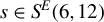
$s \in {S}^{E}(6,12)$
 for four different treatment rules.

Table 1 Long description
The table is divided into two primary sections: Case I and Case II. Each section contains 12 columns representing four treatment rules (delta super E S, delta super 1, delta super 0.5, and delta super 0) repeated for three values of alpha (0.1, 0.5, and 0.9).
* Case I:
- For alpha = 0.1 and q sub alpha (Y sub 0) = 0.1: Max regret is 0.9 for delta super E S, 0.1 for delta super 1, and 0.9 for delta super 0.5 and delta super 0. Mean regret is 0.08, 0.04, 0.14, and 0.1 respectively.
- For alpha = 0.1 and q sub alpha (Y sub 0) = 0.5: Max regret is 0.5 for all rules. Mean regret ranges from 0 to 0.43.
- For alpha = 0.1 and q sub alpha (Y sub 0) = 0.9: Max regret is 0.9 for the first three rules and 0.1 for delta super 0. Mean regret is 0.9, 0.75, 0.75, and 0.
- For alpha = 0.5 and q sub alpha (Y sub 0) = 0.1: Max regret is 0.1 for delta super E S and delta super 1, and 0.9 for delta super 0.5 and delta super 0.
- For alpha = 0.9 and q sub alpha (Y sub 0) = 0.9: delta super 0 shows the lowest max regret at 0.1 and mean regret at 0.04.
* Case II:
- This section follows the same structure as Case I with slight variations in values.
- For alpha = 0.9 and q sub alpha (Y sub 0) = 0.1: Max regret is 0 for delta super E S and 0.1 for delta super 1.
- For alpha = 0.9 and q sub alpha (Y sub 0) = 0.5: Max regret is 0.02 for delta super E S and 0.5 for the others.
- For alpha = 0.9 and q sub alpha (Y sub 0) = 0.9: Max regret is 0.03 for delta super E S and 0.1 for delta super 0.
Bolded values indicate the lowest regret achieved for specific parameters.
Proportion (in %) of states
$s\in S^{E}(6,12)$
 for which regret for the empirical success rule
${\delta }^{ES}$
 is smaller than regret of non-data rules
$\delta \in \{{\delta }^{1},\delta ^{0.5},{\delta }^{0}\}$
 .

Table 2 Long description
The table presents data for Case I and Case II across ten columns. The first column lists the parameters alpha and the quantile function q sub alpha of Y sub 0. The remaining nine columns are grouped into three sets of three, corresponding to alpha equals 0.1, 0.5, and 0.9. Each set contains sub-columns for delta super 1, delta super 0.5, and delta super 0.
* Case I Data:
- For q sub alpha of Y sub 0 equals 0.1: Prop of R of delta super E S, s less than R of delta, s ranges from 0 to 100. Prop of R of delta super E S, s less than or equal to R of delta, s ranges from 56.9 to 100.
- For q sub alpha of Y sub 0 equals 0.5: Prop of R of delta super E S, s less than R of delta, s ranges from 0 to 91.7. Prop of R of delta super E S, s less than or equal to R of delta, s ranges from 8.3 to 99.5.
- For q sub alpha of Y sub 0 equals 0.9: Prop of R of delta super E S, s less than R of delta, s ranges from 0 to 43.1. Prop of R of delta super E S, s less than or equal to R of delta, s ranges from 0 to 66.7.
* Case II Data:
- For q sub alpha of Y sub 0 equals 0.1: Prop of R of delta super E S, s less than R of delta, s ranges from 0 to 100. Prop of R of delta super E S, s less than or equal to R of delta, s ranges from 73.0 to 100.
- For q sub alpha of Y sub 0 equals 0.5: Prop of R of delta super E S, s less than R of delta, s ranges from 2.2 to 91.7. Prop of R of delta super E S, s less than or equal to R of delta, s ranges from 65.3 to 100.
- For q sub alpha of Y sub 0 equals 0.9: Prop of R of delta super E S, s less than R of delta, s ranges from 43.1 to 99.6. Prop of R of delta super E S, s less than or equal to R of delta, s ranges from 43.1 to 100.
Table 1 provides results for maximal and mean regret over all 18,564 states of nature
$s\in S^{E}(6,12)$
 for the four different treatment rules. Results for rules that are minimax regret in a given setting are reported in bold.
We first discuss results for maximal regret. The treatment rules that are known to be minimax regret for unrestricted
$\mathbb {S}$
 also have smallest maximal regret over
${\mathbb {S}}^{E}(n,w)$
 (relative to the other treatment rules considered here) for all cases except for case II) with
$\alpha $
 = 0.9, when
$q_{\alpha }(Y_{0})$
 = 0.1 (in which case,
$\delta ^{ES}$
 has smaller maximal regret than the optimal rule
$\delta ^{1})$
 , when
$q_{\alpha }(Y_{0})$
 = 0.5 (in which case, it is known that all four rules are optimal but in finite samples for
${\mathbb {S}}^{E}(n,w)$
 again
$\delta ^{ES}$
 does best), and finally when
$q_{\alpha }(Y_{0})$
 = 0.9 (in which case,
$\delta ^{ES}$
 has smaller maximal regret than the optimal rule
$\delta ^{0})$
 . The explanation is of course that
${\mathbb {S}}^{E}(n,w)$
 does not contain those states of nature that would inflict the highest regret on
$\delta ^{ES}$
 (like the particular Bernoulli and discrete distributions for
$Y_{0}$
 and
$Y_{1},$
 respectively, that are used in the proof of Proposition 1(iii)). Furthermore, reported finite sample maximal regret over
${\mathbb {S}}^{E}(n,w)$
 for the optimal rules matches the theoretical value
$\min \{q_{\alpha } (Y_{0}),1-q_{\alpha }(Y_{0})\}$
 reported in Proposition 1(iii) except for case II) with
$\alpha $
 = 0.9 when
$q_{\alpha }(Y_{0})$
 = 0.5 where the optimal rule
$\delta ^{ES}$
 has maximal regret smaller than 0.5 (which occurs, again, because
${\mathbb {S}}^{E}(n,w)$
 is not rich enough). An open question from Proposition 1(iii) is whether for
$q_{\alpha }(Y_{0})\, <$
 0.5 other minimax regret rules besides
$\delta ^{1}$
 might exist. The simulations for
$q_{\alpha }(Y_{0})$
 = 0.1 are compatible with the possibility that when
$\alpha $
 = 0.5 or 0.9 also
$\delta ^{ES}$
 might be minimax regret.
We next discuss results for mean regret. In most cases where
$q_{\alpha } (Y_{0})\in \{0.1,0.9\}$
 in which case either
$\delta ^{0}$
 or
$\delta ^{1}$
 are minimax regret, their mean performance is also best (or very close to best) among the four treatment rules. On the other hand, when
$q_{\alpha }(Y_{0})$
 = 0.5 (in which case all four treatment rules are minimax regret according to Proposition 1(iii)) we see huge differences in mean performance across the four treatment rules for a given case I) or II) and
$\alpha ,$
 but also huge differences in performance for a given treatment rule and
$\alpha $
 across cases I) and II). With respect to the former point, in case I), when
$\alpha $
 = 0.1, mean regret for the four rules is in the interval [0,0.43]. With regards to the latter point, for example, for
$\delta ^{ES}$
 , when
$\alpha $
 = 0.1, mean regret equals 0.43 and 0.06, in cases I) and II), respectively. Differences across cases I) and II) are also often huge for other quantiles. For example, again for
$\delta ^{ES}$
 , when
$q_{\alpha }(Y_{0})$
 = 0.9 and
$\alpha $
 = 0.1, mean regret equals 0.9 and 0, in cases I) and II), respectively. (Recall that we round results to the second digit. When
$q_{\alpha }(Y_{0})$
 = 0.9 and
$\alpha $
 = 0.1, there are not many distributions for
$Y_{1}$
 in
$\mathbb {S} ^{E}(n,w)$
 that have an
$\alpha $
 -quantile that exceeds 0.9.)
We next discuss the results for exercise d) contained in Table 2 where we report the proportion of the 18,564 states of nature
$s\in S^{E}(6,12)$
 for which the regret of
$\delta ^{ES}$
 is smaller than the regret of
$\delta $
 where we consider all
$\delta $
 from the set of no-data rules
$\{\delta ^{1},\delta ^{.5},\delta ^{0}\}$
 . The results indicate that for many states
$s$
 , choices of
$q_{\alpha }(Y_{0})$
 ,
$\alpha ,$
 and the distribution for
$Y_{0},\, R(\delta ^{ES},s)$
 , and
$R(\delta ,s)$
 are very close which leads to numerically unstable results. To deal with the instability, we introduce the buffer
$\xi $
 as explained above and
$Prop(R(\delta ^{ES},s)<R(\delta ,s))$
 and
$Prop(R(\delta ^{ES},s)\leq R(\delta ,s))$
 in Table 2 represent the proportion of states
$s$
 for which
$R(\delta ^{ES},s)<R(\delta ,s)-\xi $
 and
$R(\delta ^{ES},s)<R(\delta ,s)+\xi ,$
 respectively. Those two proportions can be drastically different, suggesting that, in many scenarios, regrets for
$\delta ^{ES}$
 and
$\delta $
 are (virtually) identical. According to the measure
$Prop(R(\delta ^{ES},s)\leq R(\delta ,s)),$
 maybe somewhat surprisingly given the results from Table 1,
$\delta ^{ES}$
 is to be preferred over the other three rules in all scenarios considered in Case II) (except the case
$\alpha =q_{\alpha }(Y_{0})$
 = 0.9 for
$\delta ^{0})$
 and in the majority of scenarios in Case I) (except compared to
$\delta ^{0}$
 when
$q_{\alpha }(Y_{0})$
 = 0.5,
$\alpha $
 = 0.1 and except for most cases with
$q_{\alpha }(Y_{0})$
 = 0.9 and all three rules
$).$
 Quite often
$Prop(R(\delta ^{ES},s)\leq R(\delta ,s))$
 is reported as higher than 95%, but the improvement in regret for many states of nature is minuscule. For example, compared to
$\delta ^{0.5}$
 in Case I) with
$\alpha =q_{\alpha }(Y_{0})$
 = 0.1 only in 33.3% of the cases
$(R(\delta ^{ES},s)<R(\delta ,s))$
 while for 100% of the cases
$(R(\delta ^{ES},s)\leq R(\delta ,s))$
 implying that the regret of
$\delta ^{ES}$
 in 66.7% of the cases is at most
$\xi $
 smaller than the regret of
$\delta ^{0.5}$
 .
3 TREATMENT CHOICE WITH A COVARIATE
As in Stoye (Reference Stoye2009) we next allow for a discrete covariate
$X\in \mathcal {X}=\{x_{1},\ldots ,x_{K}\}$
 that is observed both in the sample and in the treatment data. Outcomes
$Y_{t,x}$
 now carry a double subindex to indicate the treatment status
$t\in \{0,1\}$
 and the value of the covariate
$x\in \mathcal {X}.$
 It is assumed that
$x_{k}$
 occurs with positive probability for each
$k=1,\ldots ,K.$
 Denote by
$F_{X}$
 the distribution of
$X.$
 A state of the world
$s\in \mathbb {S}$
 now represents a joint distribution for
$(Y_{t,x})_{t\in \{0,1\},\text { }x\in \mathcal {X}}.$

A sample
$w=w_{N}$
 now consists of realizations
$(t_{i},x_{i},y_{i})$
 for
$i=1,\ldots ,N$
 of
$(T,X,Y_{T,X}),$
 where
$y_{i}$
 is a realization of
$Y_{t_{i},x_{i}}$
 , and we consider again sampling designs (i)–(iii) from Section 2.2. It is assumed that
$x_{i},\, i=1,\ldots ,N,$
 are i.i.d. and
$F_{X}$
 is independent of
$s$
 and
$T$
 .
In design (i), “fixed number of treated/untreated units,” there are
$N_{0}$
 observations
$(0,x_{i},y_{i})$
 with
$y_{i}$
 being i.i.d. draws of
$Y_{0,x_{i}},\, i=1,\ldots ,N_{0}$
 and
$N_{1}=N-N_{0}$
 observations
$(1,x_{i},y_{i})$
 with
$y_{i}$
 being i.i.d. draws of
$Y_{1,x_{i}},\, i=N_{0}+1,\ldots ,N.$
 Note that there are not typically equally many treated and untreated observations for each covariate
$x_{k},\, k=1,\ldots ,K.$
 In fact, there may be zero observations altogether in the sample for a given
$x_{k}.$

In design (ii), “random sampling,” the observations
$(t_{i},x_{i},y_{i})$
 for
$i=1,\ldots ,N$
 are i.i.d. realizations of
$(T,X,Y_{T,X})$
 with
$P(T_{i}=1)=p\in (0,1)$
 with
$T,X$
 , and the potential outcomes (whose distribution is
$s$
 ) being independent of each other.
In design (iii), “testing an innovation,”
$(1,x_{i},y_{i})$
 for
$i=1,\ldots ,N$
 are observed, where
$y_{i}$
 is an independent realization of
$Y_{1,x_{i}},$
 for
$i=1,\ldots ,N.$

In design (iii), we assume the DM knows the
$\alpha $
 -quantile, denoted by
$q_{\alpha }(Y_{0,X}),$
 of
$Y_{0,X}$
 and nature can choose from joint distributions
$s\in \mathbb {S}$
 for
$(Y_{t,x})_{t\in \{0,1\},\text { } x\in \mathcal {X}}$
 such that the
$\alpha $
 -quantile of
$Y_{0,X}$
 equals
$q_{\alpha }(Y_{0,X}).$

A treatment rule
$\delta $
 maps a sample
$w_{N}$
 onto treatment probabilities for each
$x_{k}$
 for
$k=1,\ldots ,K,$
 that is,
$\delta (w_{N})\in \lbrack 0,1]^{K},$
 where the
$k$
 -th component of
$\delta (w_{N})$
 indicates the treatment probability for individuals with covariate
$x_{k}$
 for
$k=1,\ldots ,K.$
 Denote the
$k$
 -th component of
$\delta (w_{N})$
 by
$\delta _{x_{k}}(w_{N})$
 for
$k=1,\ldots ,K.$
 With some abuse of notation, for each design (i)–(iii), we denote the set of all treatment rules by the same symbol
$\mathbb {D}$
 (even though it means something different for different designs).
The object of interest is

the
$\alpha $
 -quantile of the outcome distribution. With that definition, regret is then defined formally analogously to the setup without a covariate, namely,
$R(\delta ,s)=\sup _{d\in \mathbb {D}}u(d,s)-u(\delta ,s).$
 Alternatively, one could focus on the
$\alpha $
 -quantile of the outcome distribution for a particular covariate only,
$x_{1}$
 say,
$u_{x_{1}}(\delta ,s)=q_{s,F_{X} ,\alpha }(Y_{B(\delta _{x_{1}}(w_{N})),x_{1}})$
 and obtain analogous results to the ones in Corollary 2 below.
If the space of probability distributions for nature
$\mathbb {S}$
 is unrestricted and thus equals the space of all distributions for
$(Y_{t,x} )_{t\in \{0,1\},\text { }x\in \mathcal {X}}$
 one can show in designs (i) and (ii) (as an implication of the proof of Proposition 1) that for every treatment rule
$\delta $
 maximal regret over
$\mathbb {S}$
 equals 1,
$\max _{s\in \mathbb {S} }R(\delta ,s)=1$
 . This result then immediately implies that every treatment rule is minimax regret. The corollary (to Proposition 1) that follows gives a stronger result; it shows that maximal regret continues to be 1 even if certain restrictions are imposed on
$\mathbb {S}$
 . For simplicity of the presentation, assume
$\alpha \in (0,1).$

Corollary 2.
$(i)$
 and
$(ii)$
 . In the case of the designs “fixed number of treated/untreated units” and “random sampling” for any treatment rule
$\delta \in \mathbb {D}$
 ,
$\max _{s\in \mathbb {S}}R(\delta ,s)=1$
 if
$\mathbb {S}$
 includes as a subset all joint distributions for
$(Y_{t,x} )_{t\in \{0,1\},\text { }x\in \mathcal {X}}$
 whose marginals are independent Bernoulli distributions. Therefore, any
$\delta \in \mathbb {D}$
 is minimax regret.
$(iii)$
 In the case of “testing an innovation” assume the DM knows the
$\alpha $
 -quantile, denoted by
$q_{\alpha }(Y_{0,X}),$
 of
$Y_{0,X}.$
 If
$q_{\alpha }(Y_{0,X})=1/2,$
 then any
$\delta \in \mathbb {D}$
 is minimax regret; if
$q_{\alpha }(Y_{0,X})>1/2,$
 then
$\delta ^{0}=0$
 is the unique minimax regret rule, and if
$q_{\alpha }(Y_{0,X})<1/2,$
 then
$\delta ^{1}=1$
 is a minimax regret rule. In each case,
$max_{s\in \mathbb {S}}R(\delta ,s)=\min \{q_{\alpha }(Y_{0,X}),1-q_{\alpha }(Y_{0,X})\}$
 .
Comments: 1. Various variants could be considered in design (iii). For example, one could instead assume that the joint distribution
$(Y_{0,x} )_{x\in \mathcal {X}}$
 is known (in which case nature only chooses a joint distribution for
$(Y_{1,x})_{x\in \mathcal {X}})$
 or one could assume that the DM knows the vector
$(q_{\alpha }(Y_{0,x_{1}}),\ldots ,q_{\alpha }(Y_{0,x_{K}}))$
 of
$\alpha $
 -quantiles of all the marginal distributions
$(Y_{0,x})_{x\in \mathcal {X}}$
 and nature can choose from joint distributions
$s\in \mathbb {S}$
 for
$(Y_{t,x})_{t\in \{0,1\},\text { }x\in \mathcal {X}}$
 such that all the marginals
$(Y_{0,x})_{x\in \mathcal {X}}$
 have the required
$\alpha $
 -quantiles.
2. One could also consider alternative sampling designs (i)–(iii), where in the sampling stage, rather than being randomly assigned, the values of the covariate
$X$
 are assigned deterministically, as is done for treatment status in design (i). This could be referred to as “stratified sampling.”
For brevity, we do not explicitly deal with these variations.
4 CONCLUSION
We derive minimax regret treatment rules in finite samples when an
$\alpha $
 -quantile of the outcome distribution is the focus of interest. We establish that when the sample i) consists of a fixed number of untreated/treated units or ii) is generated via random treatment assignment then all treatment rules are minimax regret and therefore the minimax regret criterion is not helpful in singling out a recommended treatment rule. Given that the same shortcoming applies to the max–min criterion, an important question concerns finding a meaningful criterion in this setup based on which an optimal treatment rule should be chosen. The idea from Montiel Olea et al. (Reference Montiel Olea, Qiu and Stoye2026) to look for rules that randomize “the least” in a situation where there are multiple minimax regret rules would not lead to a unique rule in our setup because in cases i) and ii) both
$\delta ^{0}$
 and
$\delta ^{1}$
 are minimax regret and never randomize. Given all these facts, it seems reasonable to simply adopt a rule that is minimax regret optimal when regret is based on the notion of expected welfare (in particular, such a rule is optimal according to criterion (2.7)).
We also establish that when iii) the sample consists of only realizations from the treated population while the
$\alpha $
 -quantile of the untreated population is known, never treating is the unique minimax rule if the known quantile exceeds 0.5, while always treating is a minimax rule if that quantile is strictly smaller than 0.5, and finally, if the quantile equals 0.5, then any treatment rule is minimax regret. It follows that based on the minimax regret criterion, rules that take the data into consideration are never strictly preferred.
An interesting but quite difficult extension concerns applying the minimax regret criterion in finite samples to CVaR, defined as
$S_{s,\alpha }(Y):=\alpha ^{-1}E_{s}[Y1(Y\leq q_{s,\alpha }(Y))]$
 for a random variable
$Y$
 rather than to the
$\alpha $
 -quantile of
$Y$
 .Footnote
9
Another extension involves modifying the analysis in Huang and Guggenberger (Reference Huang and Guggenberger2025) that considers pilot data from a setup where the objective is expected outcome to one where the objective is a quantile.
A APPENDIX
A.1 Proof of Proposition 1
We use the notation
$P_{s}(A)$
 to denote the probability of the event
$A$
 when nature chooses the state of the world
$s\in \mathbb {S}$
 and we write shorthand
$w$
 instead of
$w_{N}$
 for the sample of size
$N$
 . Note that, for a state of the world
$s\in \mathbb {S}$
 and treatment rule
$\delta \in \mathbb {D,}$


and analogously for
$P_{s}(Y_{B(\delta (w))}\geq q)$
 , where the second equality uses independence. By definition, an
$\alpha $
 -quantile
$q$
 of
$Y_{B(\delta (w))}$
 satisfies
$P_{s}(Y_{B(\delta (w))}\leq q)\geq \alpha $
 and
$P_{s} (Y_{B(\delta (w))}\geq q)\geq 1-\alpha .$

The proofs of (i) and (ii) proceed by showing that for any treatment rule
$\delta \in \mathbb {D,}$
 there exists a state of the world
$s_{\delta } \in \mathbb {S}$
 for which
$R(\delta ,s_{\delta })=1.$
 Because it is also true that for any treatment rule
$\delta \in \mathbb {D},\, \max _{s\in \mathbb {S} }R(\delta ,s)\leq 1,$
 it follows that any treatment rule is minimax.
Lemma 3(ii) below establishes the (unsurprising) result that for any arbitrary
$s\in \mathbb {S,}$


This result implies a simplified formula for
$R(\delta ,s)$
 that we will use from now on.
In the proof of (i) and (ii) that follows, for any given treatment rule
$\delta \in \mathbb {D}$
 , we will construct an
$s_{\delta }\in \mathbb {S}$
 for which
$\max \{q_{s_{\delta },\alpha }(Y_{0}),q_{s_{\delta },\alpha }(Y_{1})\}=1$
 and
$u(\delta ,s_{\delta })=0.$
 Namely, throughout the proof of (i) and (ii) for an arbitrary treatment rule
$\delta \in \mathbb {D,}$
 we construct an
$s_{\delta } \in \mathbb {S}$
 whose independent marginals for
$Y_{0}$
 and
$Y_{1}$
 are Bernoulli (supported on
$\{0,1\}$
 ) and for which
$R(\delta ,s_{\delta })=1$
 . Under these restrictions, the distribution
$s_{\delta }$
 for
$(Y_{0},Y_{1})$
 is then fully defined by

The
$\alpha $
 -quantiles of
$Y_{0},\, Y_{1},$
 and
$Y_{B(\delta (w))}$
 in the constructions below will be unique when
$\alpha \in (0,1)$
 . Therefore, the particular value of
$r\in \lbrack 0,1]$
 has no impact on the results.
Part (i). As in (A.1) and with
$s_{\delta }$
 just defined

where for a vector
$u\in \{0,1\}^{N_{0}}$
 , we denote by
$\overline {u} \in \mathbb {N}$
 the sum of its components (i.e., the number of 1’s in the vector) and similarly for other vectors, and

Note that in the second line of (A.4), the term
$a_{0} ^{N_{0}-\overline {u}}(1-a_{0})^{\overline {u}}a_{1}^{N_{1}-\overline {v} }(1-a_{1})^{\overline {v}}$
 is the probability to observe particular vectors
$u$
 and
$v$
 while the term
$\delta ((u^{\prime },v^{\prime })^{\prime } )a_{1}+(1-\delta ((u^{\prime },v^{\prime })^{\prime }))a_{0}$
 is the probability that an outcome 0 is reached when the sample consists of
$u$
 and
$v.$

Assume
$\alpha \in (0,1)$
 first. When in the definition of
$s_{\delta }$
 in (A.3), we take
$(a_{0},a_{1})=(1,\alpha )$
 we obtain from (A.4),

Given that the coefficient
$\alpha ^{N_{1}-j}(1-\alpha )^{j}(\alpha -1)$
 in front of
$\delta ^{0,j}$
 is negative (noting that
$\alpha \in (0,1)),$
 it follows that
$P_{s_{\delta }}(Y_{B(\delta (w))}=0)$
 is strictly decreasing in each
$\delta ^{0,j}.$
 Therefore, we obtain

where the right-hand bound follows from (A.6) by replacing
$\delta ^{0,j}$
 by its maximal value
$\binom {N_{1}}{j}.$

Consider first the case where at least one of the
$\delta ^{0,j}$
 (for
$j=0,\ldots ,N_{1}$
 ) is smaller than
$\binom {N_{1}}{j}.$
 In that case, it follows that
$P_{s_{\delta }}(Y_{B(\delta (w))}=0)>\alpha .$
 Furthermore, notice that
$P_{s_{\delta }}(Y_{B(\delta (w))}=0)$
 is continuous in
$a_{1}$
 and therefore
$P_{s_{\delta }}(Y_{B(\delta (w))}=0)>\alpha $
 when instead of
$(a_{0} ,a_{1})=(1,\alpha ),\, s_{\delta }$
 is taken as
$(a_{0},a_{1})=(1,\alpha -\varepsilon )$
 for some small enough
$\varepsilon>0.$
 But then for that choice of
$s_{\delta },\, u(\delta ,s_{\delta })=0$
 and
$\max \{q_{s_{\delta },\alpha }(Y_{0}),q_{s_{\delta },\alpha }(Y_{1})\}=q_{s_{\delta },\alpha }(Y_{1})=1.$
 Therefore,
$R(\delta ,s_{\delta })=1$
 as desired.
Next, consider the case where
$\delta ^{0,j}=\binom {N_{1}}{j}$
 for all
$j=0,\ldots ,N_{1}$
 (which implies that
$\delta ((0^{N_{0}\prime },v^{\prime })^{\prime })=1$
 for all
$v\in \{0,1\}^{N_{1}},$
 where
$0^{N_{0}}$
 denotes an
$N_{0}$
 -dimensional column vector of zeros). In that case, from (A.4), we obtain with
$(a_{0},a_{1})=(\alpha ,1)$


where the second equality uses
$\delta ^{0,0}=\binom {N_{1}}{0}=1,$
 the first inequality follows from setting
$\delta ^{i,0}=0$
 for
$i=1,\ldots ,N_{0},$
 and the second inequality follows from
$\alpha \in (0,1).$
 The remainder of the proof is as above, namely, by continuity
$P_{s_{\delta }}(Y_{B(\delta (w))}=0)>\alpha $
 for an
$s_{\delta }$
 with
$(a_{0},a_{1})=(\alpha -\varepsilon ,1)$
 for a small enough
$\varepsilon>0.$
 For such
$s_{\delta }$
 , regret equals 1.
Now consider the case
$\alpha =0.$
 Take any
$\delta $
 and define
$s_{\delta }$
 by setting
$a_{0}=P_{s_{\delta }}(Y_{0}=0)=0$
 and
$a_{1}=P_{s_{\delta }} (Y_{1}=0)=\varepsilon>0.$
 Then,
$q_{s_{\delta },0}(Y_{1})=0$
 and any
$q\in \lbrack 0,1]$
 satisfies the condition in (2.4) for
$X=Y_{0}.$
 Thus, with
$r=1,$
 the
$0$
 -quantile of
$Y_{0}$
 equals 1. Thus, in order for regret to equal 1 under
$s_{\delta }$
 , it is enough to establish that the
$0$
 -quantile of
$Y_{B(\delta (w))}$
 equals 0. The latter follows if
$P_{s_{\delta }}(Y_{B(\delta (w))}=0)>0.$
 From (A.4),

with
$\delta ^{N_{0},j}= {\textstyle \sum \nolimits _{v\in \{0,1\}^{N_{1}},\text { }\overline {v}=j}} \delta ((1,\ldots ,1,v^{\prime })^{\prime }).$
 If
$P_{s_{\delta }}(Y_{B(\delta (w))}=0)>0,$
 the proof is complete. If not, and
$P_{s_{\delta }}(Y_{B(\delta (w))}=0)=0,$
 it must be that
$\delta ((1,\ldots ,1,v^{\prime })^{\prime })=0$
 for all
$v\in \{0,1\}^{N_{1}}.$
 If
$\delta ((1,\ldots ,1,v^{\prime })^{\prime })=0$
 for all
$v\in \{0,1\}^{N_{1}}$
 , define
$s_{\delta }^{\prime }$
 by setting
$a_{0} =P_{s_{\delta }^{\prime }}(Y_{0}=0)=\varepsilon $
 and
$a_{1}=P_{s_{\delta }^{\prime }}(Y_{1}=0)=0.$
 Then, by (A.4), with
$\delta ^{i,N_{1}}= {\textstyle \sum \nolimits _{u\in \{0,1\}^{N_{0}},\overline {u}=i}} \delta ((u^{\prime },1,\ldots ,1)^{\prime })\leq \binom {N_{0}}{i}$
 ,

But
$1-\delta ((1,\ldots ,1,v^{\prime })^{\prime })=1$
 for all
$v\in \{0,1\}^{N_{1}}$
 implies
$\binom {N_{0}}{i}-\delta ^{i,N_{1}}=1$
 when
$i=N_{0}.$
 Thus, by (A.10),
$P_{s_{\delta }^{\prime }}(Y_{B(\delta (w))}=0)>0.$
 But, the latter implies that regret equals 1 under
$s_{\delta }^{\prime }. $

Finally, consider the case
$(\alpha =1$
 and
$r=0).$
 Consider a treatment rule
$\delta $
 that is not equal to 1 wp1 and not equal to 0 wp1. We will show that
$\max _{s\in \mathbb {S}}R(\delta ,s)=0.$
 To see this, fix
$s\in \mathbb {S}.$
 By the definition of an
$\alpha $
 -quantile in (2.4) and the choice
$r=0$
 note that, for any
$q<q_{s,1}(Y_{0}),$
 it must be that
$P_{s} (Y_{0}\leq q)<1,$
 and likewise for any
$q<q_{s,1}(Y_{1}),$
 it must be that
$P_{s}(Y_{1}\leq q)<1.$
 Therefore, using (A.1), for any
$q<\max \{q_{s,1}(Y_{0}),q_{s,1}(Y_{1})\}$
 , we have

which implies
$q<q_{s,1}(Y_{B(\delta (w))}).$
 By Lemma 3,
$q_{s,1}(Y_{B(\delta (w))})\leq \max \{q_{s,1}(Y_{0}),q_{s,1}(Y_{1})\}$
 and thus
$q_{s,1}(Y_{B(\delta (w))})=\max \{q_{s,1}(Y_{0}),q_{s,1}(Y_{1})\}$
 . But that implies that
$R(\delta ,s)=0$
 and because
$s\in \mathbb {S}$
 that proves the desired result
$.$

Part (ii). The proof of (ii) is similar to case (i). Again we start off with
$\alpha \in (0,1)$
 and define
$s_{\delta }$
 as in (A.3). We obtain

where for given vectors
$t\in \{0,1\}^{N}$
 and
$y\in \{0,1\}^{N},\, N_{0ty}$
 denotes the number of
$y_{t_{i}},\, i=1,\ldots ,N,$
 for which
$y_{t_{i}}=0$
 and
$t_{i}=0,\, N_{1ty}$
 is the number of
$y_{t_{i}},\, i=1,\ldots ,N,$
 for which
$y_{t_{i}}=0$
 and
$t_{i}=1,$
 where again
$\overline {t}\in \mathbb {N}$
 for a vector
$t\in \{0,1\}^{N}$
 denotes the sum of its components, and

Note that
$N_{0ty}\leq N-\overline {t}$
 and
$N_{1ty}\leq \overline {t}.$
 In the second line of (A.11), the factor
$p^{\overline {t} }(1-p)^{N-\overline {t}}$
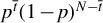 captures the probability of observing exactly
$\overline {t}$
 treatments and
$N-\overline {t}$
 controls in the sample, while the factor
$a_{0}^{N_{0ty}}(1-a_{0})^{N-\overline {t}-N_{0ty}}$
 captures the probability that among the
$N-\overline {t}$
 observations from the control group exactly
$N_{0ty}$
 zeros are observed, while, finally, the factor
$a_{1}^{N_{1ty}}(1-a_{1})^{\overline {t}-N_{1ty}}$
 captures the probability that among the
$\overline {t}$
 observations from treated individuals exactly
$N_{1ty}$
 zeros are observed.
Evaluating
$P_{s_{\delta }}(Y_{B(\delta (w))}=0)$
 when
$s_{\delta }$
 takes
$(a_{0},a_{1})=(1,\alpha ),$
 we obtain

Because
$(\alpha -1)<0$
 and
$\alpha>0$
 ,
$P_{s_{\delta }}(Y_{B(\delta (w))}=0)$
 is strictly decreasing in
$\delta ^{T,N-T,j}$
 for all
$T=0,\ldots ,N$
 and
$j=0,\ldots ,T$
 and is minimized when
$\delta ^{T,N-T,j}$
 takes on its maximal value
$\binom {N}{T}\binom {T}{j}$
 . Therefore,

If
$\delta ^{T,N-T,j}<\binom {N}{T}\binom {T}{j}$
 for any
$T=0,\ldots ,N$
 and
$j=0,\ldots ,T,$
 then by an argument as in part (i), it follows that an
$s_{\delta }$
 with
$(a_{0},a_{1})=(1,\alpha -\varepsilon )$
 for
$\varepsilon>0$
 small enough leads to regret of 1. This holds because for that
$s_{\delta }$
 we have
$q_{s_{\delta },\alpha }(Y_{0})=0,\, q_{s_{\delta },\alpha }(Y_{1})=1,$
 and
$q_{s_{\delta },\alpha }(Y_{B(\delta (w))})=0.$

If on the other hand,
$\delta ^{T,N-T,j}=\binom {N}{T}\binom {T}{j}$
 for all
$T=0,\ldots ,N$
 and
$j=0,\ldots ,T,$
 then, as in part (i), one can show that
$s_{\delta }$
 defined by
$(a_{0},a_{1})=(\alpha -\varepsilon ,1)$
 for a small enough
$\varepsilon>0$
 leads to regret of 1. Namely, for
$s_{\delta }$
 with
$(a_{0},a_{1})=(\alpha ,1)$
 , we get from (A.11)

where the second equality simply takes the last summand with index
$i=N-T$
 out of the second summation sign and uses
$\delta ^{T,N-T,T}=\binom {N}{T}$
 , the inequality is obtained by setting
$\delta ^{T,i,T}=0$
 for all
$T=0,\ldots ,N$
 and
$i=0,\ldots ,N-T-1,$
 and the strict inequality uses
$\alpha ^{N-T}+\alpha (1-\alpha ^{N-T})>\alpha .$
 By an argument as in part (i), (A.15) implies that for
$s_{\delta }^{\prime }$
 with
$(a_{0},a_{1})=(\alpha -\varepsilon ,1)$
 with sufficiently small
$\varepsilon>0$
 regret of 1 can be obtained because, under
$s_{\delta }^{\prime }$
 , we have
$q_{s_{\delta }^{\prime },\alpha }(Y_{0})=1,\, q_{s_{\delta }^{\prime },\alpha }(Y_{1})=0,$
 and
$q_{s_{\delta }^{\prime },\alpha }(Y_{B(\delta (w))} )=0.$

Next, assume
$\alpha =0.$
 Define
$s_{\delta }$
 such that
$a_{0}=P_{s_{\delta } }(Y_{0}=0)=0$
 and
$a_{1}=P_{s_{\delta }}(Y_{1}=0)=\varepsilon>0.$
 That and
$r=1$
 imply that
$q_{s_{\delta },\alpha }(Y_{0})=1$
 and
$q_{s_{\delta },\alpha }(Y_{1})=0.$
 Then, from (A.11),

Thus,
$P_{s_{\delta }}(Y_{B(\delta (w))}=0)>0$
 (which implies
$R(\delta ,s_{\delta })=1$
 ), unless
$\delta ((t,y))=0$
 for all vectors
$t,y\in \{0,1\}^{N}$
 such that
$y_{t_{j}}=1$
 if
$t_{j}=0$
 for
$j=1,\ldots ,N.$
 For such
$\delta $
 consider instead
$s_{\delta }^{\prime }$
 such that
$a_{0}=P_{s_{\delta } ^{\prime }}(Y_{0}=0)=\varepsilon>0$
 and
$a_{1}=P_{s_{\delta }^{\prime }} (Y_{1}=0)=0.$
 Then

exceeds zero, because
$1-\delta ((0^{N\prime },1^{N^{\prime }})^{\prime })=1$
 and the vectors
$t=0^{N}$
 and
$y=1^{N}$
 appear in the sum in (A.17)
$.$
 Thus,
$R(\delta ,s_{\delta }^{\prime })=1.$

Finally, the case
$(\alpha =1$
 and
$r=0)$
 is handled exactly as in part (i).
Part (iii). We first show the following lemma
Lemma 1. Let
$(\alpha \in (0,1)$
 and
$r\in \lbrack 0,1])$
 or
$(\alpha =0$
 and
$r=1).$
 If
$\delta \neq 0,$
 then there exists an
$s_{\delta } \in \mathbb {S}$
 such that
$R(\delta ,s_{\delta })=q_{\alpha }(Y_{0}).$

A.2 Proof of Lemma 1
The case
$q_{\alpha }(Y_{0})=0$
 is trivial. Simply take
$s_{\delta }$
 such that
$P_{s_{\delta } }(Y_{0}=0)=P_{s_{\delta }}(Y_{1}=0)=1.$
 Thus, from now on, we assume
$q_{\alpha }(Y_{0})>0.$

Assume first
$\alpha \in (0,1).$
 Because
$\delta \neq 0,$
 there exists a vector

where
$y_{1,i}\in \lbrack 0,1]$
 for
$i=1,\ldots ,N.$
 (When
$N=0,$
 then we don’t need to define
$\widetilde {w}).$

Definition of Distributions of
$Y_{0}$
 and
$Y_{1}:$
 We now define an
$s_{\delta }\in \mathbb {S}$
 for which
$R(\delta ,s_{\delta })=q_{\alpha }(Y_{0})$
 and under
$s_{\delta }\in \mathbb {S}$
 ,
$Y_{0}$
 and
$Y_{1}$
 have independent discrete marginals. Namely,
$Y_{0}$
 is defined by
$P_{s_{\delta }}(Y_{0}=0)=\alpha -\varepsilon $
 for some small
$\varepsilon>0\, ($
 and obviously
$\varepsilon <\alpha )$
 to be further restricted below and
$P_{s_{\delta }}(Y_{0}=q_{\alpha }(Y_{0}))=1-(\alpha -\varepsilon ).$
 Thus,
$q_{s_{\delta },\alpha }(Y_{0})=q_{\alpha }(Y_{0})$
 .
When
$N=0,$
 set
$P_{s_{\delta }}(Y_{1}=0)=1$
 and note that
$P_{s_{\delta } }(Y_{B(\delta )}=0)=\delta +(1-\delta )(\alpha -\varepsilon )$
 which exceeds
$\alpha $
 for
$\varepsilon $
 small enough (using
$\alpha <1).$
 Thus,
$q_{s_{\delta },\alpha }(Y_{1})=0$
 and
$q_{s_{\delta },\alpha }(Y_{B(\delta )})=0$
 which implies the desired result
$R(\delta ,s_{\delta })=q_{\alpha }(Y_{0}).$

When
$N\geq 1,$
 the discrete distribution of
$Y_{1}$
 under
$s_{\delta }$
 is defined by

where the
$y_{1,i}\text{ for } i=1,\ldots ,N$
 appear as the components of
$\widetilde {w}$
 in (A.18). Note that all probabilities in (A.19) are properly defined, that is, they are all in the interval
$(0,1]$
 , and sum up to 1. Just for clarity,
$ {\textstyle \sum \nolimits _{j=1}^{N}} I(y_{1,j}=0)$
 equals the number of zero components in the vector
$\widetilde {w}.$
 Note that several of the
$y_{1,i}$
 for
$i=1,\ldots ,N$
 may be identical and therefore
$Y_{1}$
 may be supported on strictly fewer than
$N+1$
 points.
With these definitions, we obtain
$q_{s_{\delta },\alpha }(Y_{1})=0$
 (because 0.5
$(\alpha +1)>\alpha )$
 and

where the inequality is obtained by setting
$\delta (\widehat {w})=0$
 except for when
$\widehat {w}=\widetilde {w},$
 using that
$P_{s_{\delta }}(Y_{1} =0)-P_{s_{\delta }}(Y_{0}=0)\geq \frac {\alpha +1}{2}-(\alpha -\varepsilon )>0.$
 We claim that
$P_{s_{\delta }}(Y_{B(\delta (w))}=0)>\alpha $
 (and thus
$q_{s_{\delta},\alpha }(Y_{B(\delta (w))})=0$
 ) for sufficiently small
$\varepsilon>0.$
 But the claim is equivalent to

which clearly holds true for
$\varepsilon>0$
 sufficiently small (using
$\alpha <1)$
 .
When
$\alpha =0$
 (in which case, we take
$r=1),$
 we can use the same proof structure except we use
$s_{\delta }$
 such that
$P_{s_{\delta }}(Y_{0} =q_{\alpha }(Y_{0}))=1$
 (which implies
$q_{s_{\delta },\alpha }(Y_{0})=q_{\alpha }(Y_{0}))$
 and the distribution for
$Y_{1}$
 defined in (A.19) with
$\alpha =0.\, {\square} $

Note throughout that for
$s\in \mathbb {S,}$
 we have
$q_{\alpha }(Y_{0} )=q_{s,\alpha }(Y_{0}).$

Consider first the case
$q_{\alpha }(Y_{0})>1/2.$
 For
$\delta ^{0}\equiv 0,$
 we will show next that

The statement in (A.22) follows easily because for any
$s\in \mathbb {S}$
 for which
$q_{s,\alpha }(Y_{1})=1,$
 we obtain
$R(\delta ^{0},s)=1-q_{\alpha }(Y_{0}).$
 Furthermore, because always

(as proven in Lemma 3(i) below)
$1-q_{s,\alpha }(Y_{0})$
 is the maximal possible regret for any
$s\in \mathbb {S}$
 for which
$q_{s,\alpha } (Y_{1})>q_{s,\alpha }(Y_{0}).$
 For any
$s\in \mathbb {S}$
 , such that
$q_{s,\alpha }(Y_{1})\leq q_{s,\alpha }(Y_{0})$
 regret is zero. That proves (A.22).
Because when
$q_{\alpha }(Y_{0})>1/2,$
 we have
$1-q_{s,\alpha }(Y_{0} )<q_{s,\alpha }(Y_{0}),$
 (A.22) combined with the lemma implies the desired result when
$q_{\alpha }(Y_{0})>1/2$
 .
Next, consider the case
$q_{\alpha }(Y_{0})=1/2.$
 Statement (A.22) (that also holds when
$q_{\alpha }(Y_{0})=1/2)$
 , Lemma 1, together with the fact that regret is bounded by 1/2 (by (A.23) when
$q_{s,\alpha }(Y_{0})=1/2),$
 establish that all treatment rules are minimax regret.
Finally, consider the case
$q_{\alpha }(Y_{0})<1/2.$
 We have
$\max _{s\in \mathbb {S}}R(\delta ^{\ast },s)=q_{s,\alpha }(Y_{0})$
 for
$\delta ^{\ast } =1$
 . Lemma 1 establishes that for
$\delta \neq 0\, \max _{s\in \mathbb {S}}R(\delta ,s)\geq q_{s,\alpha }(Y_{0})$
 while for
$\delta ^{0}\equiv 0,\, \max _{s\in \mathbb {S}}R(\delta ^{0},s)=1-q_{s,\alpha } (Y_{0})>q_{s,\alpha }(Y_{0}).$
 It follows that
$\delta ^{\ast }=1$
 is a minimax rule.
Finally, the case where
$\alpha =1$
 and
$r=0$
 is proven as in part (i).
${\square} $

A.3 Proof of Corollary 1
(a) This statement follows as a corollary from the proof of Proposition 1 because that proof only used Bernoulli distributions for nature for parts (i) and (ii) and discrete distributions in part (iii).
(b) (i) Consider an arbitrary treatment rule
$\delta .$
 Consider a state of nature
$s=s_{\alpha ,\varepsilon ,n}$
 for
$n\in \mathbb {N}$
 such that
$Y_{0}$
 has density
$n$
 on
$[0,1/n]$
 and
$Y_{1}$
 has density
$f=f_{\alpha ,\varepsilon ,n}$
 which equals
$n(\alpha -\varepsilon )$
 on
$[0,1/n]$
 and
$n(1-\alpha +\varepsilon )$
 on
$[1-1/n,1]$
 (and zero elsewhere) for some small
$\varepsilon \in \lbrack 0,\alpha /2]$
 to be specified more precisely below. Note that these continuous distributions are chosen in order to approximate as
$n\rightarrow \infty $
 the Bernoulli distributions used in the proof of Proposition 1(i). With these definitions,

Consider an arbitrary
$q\in (0,1).$
 Then for all
$n$
 such that
$1/n<q<1-1/n$


where
$y:=(y_{01},\ldots ,y_{0N_{0}},y_{11},\ldots ,y_{1N_{1}})^{\prime }$
 and the inequality comes from picking
$\delta ^{1}\equiv 1$
 given that
$\alpha -\varepsilon -1<0.$

Note that if
$P_{s}(\delta (w)=1)<1$
 for one choice of
$\varepsilon \in \lbrack 0,\alpha /2],$
 then it holds for any
$\varepsilon \in \lbrack 0,\alpha /2].$

Case 1:
$P_{s}(\delta (w)=1)<1$
 . By the same steps as in (A.25) with
$\varepsilon =0$
 , we obtain
$P_{s}(Y_{B(\delta (w))}\leq q)>\alpha $
 and, by continuity in
$\varepsilon $
 , then also for
$\varepsilon>0$
 sufficiently small. It follows that the
$\alpha $
 -quantile of
$Y_{B(\delta (w))}$
 is not greater than
$q$
 .
Case 2:
$P_{s}(\delta (w)=1)=1$
 . In that case, consider a state of nature
$\widetilde {s}=\widetilde {s}_{\alpha ,\varepsilon ,n}$
 for
$n\in \mathbb {N}$
 such that
$Y_{1}$
 has density
$n$
 on
$[0,1/n]$
 and
$Y_{0}$
 has density
$\widetilde {f}=\widetilde {f}_{\alpha ,\varepsilon ,n}$
 which equals
$n(\alpha -\varepsilon )$
 on
$[0,1/n]$
 and
$n(1-\alpha +\varepsilon )$
 on
$[1-1/n,1]$
 (and zero elsewhere). Thus,

and, analogously to (A.25),

where
$A_{n}:=[0,1]^{N_{0}}\backslash \lbrack 0,1/n]^{N_{0}},$
 the second equality uses that
$\delta (w)=1$
 a.s. on
$[0,1/n]^{N}$
 (under
$s$
 and therefore also under
$\widetilde {s}),$
 and the inequality is obtained by taking
$\delta (y)=0$
 on the domain of integration. If
$\varepsilon $
 was equal to zero, the final expression in (A.27) would be strictly larger than
$\alpha$
 . By continuity in
$\varepsilon $
 , that is then also true for sufficiently small
$\varepsilon>0.$
 It follows that the
$\alpha $
 -quantile of
$Y_{B(\delta (w))}$
 is not greater than
$q$
 .
As
$q$
 can be chosen arbitrarily small in that construction it follows that, both in Cases 1 and 2, regret arbitrarily close to 1 can be inflicted by nature given (A.24) and (A.26).
Parts (ii) and (iii) follow from similar constructions.
${\square} \, $

A.4 Proof of the Statements in Comment 3 below Corollary 1
Note first that
$q(\delta )$
 indeed exists because cdfs are continuous from the left. For example,
$q(0)=q_{\alpha }(Y_{0})$
 and
$q(1)=0.$
 Also note that for any
$q\in \lbrack 0,1]$
 , the function
$g(\delta ):=\delta +(1-\delta )F_{Y_{0}}(q)$
 is weakly increasing in
$\delta .$
 It follows that
$q(\delta )$
 is weakly decreasing in
$\delta .$
 Therefore,
$q_{\alpha }(Y_{0})-q(\delta )$
 is weakly increasing in
$\delta .$

If
$\delta <1,$
 then regret of
$1-q_{\alpha }(Y_{0})$
 can be achieved by nature by defining the distribution of
$Y_{1}$
 as
$P_{s}(Y_{1}=0)=\alpha -\varepsilon $
 and
$P_{s}(Y_{1}=1)=1-(\alpha -\varepsilon )$
 for some small
$\varepsilon>0$
 (to be specified further below). Namely, with that definition, for
$q_{\alpha }(Y_{0})<1,$
 we have

which exceeds
$\alpha $
 for
$\varepsilon $
 small enough because
$F_{Y_{0} }(q_{\alpha }(Y_{0}))>\alpha $
 and
$\delta <1.$
 And of course
$P_{s} (Y_{B(\delta )}\leq q_{\alpha }(Y_{0}))\geq \alpha $
 when
$q_{\alpha }(Y_{0})=1.$
 Because the
$\alpha $
 -quantile of
$Y_{B(\delta )}$
 can clearly not be smaller than
$q_{\alpha }(Y_{0})$
 it follows that it is equal to
$q_{\alpha }(Y_{0}).$

But then, in the case
$q_{\alpha }(Y_{0})<1/2,$
 it follows that for any
$\delta \in \lbrack 0,1),\, \max _{s\in \mathbb {S}}R(\delta ,s)\geq 1-q_{\alpha }(Y_{0})>q_{\alpha }(Y_{0}).$
 Given that for
$\delta ^{1}\equiv 1$
 maximal regret equals
$q_{\alpha }(Y_{0}),$
 it is the unique minimax regret rule. When
$q_{\alpha }(Y_{0})=1/2,$
 regret cannot exceed 1/2 and given regret of
$1-q_{\alpha }(Y_{0})$
 can always be achieved by the argument above (for
$\delta <1$
 and for
$q_{\alpha }(Y_{0})=1/2$
 also for
$\delta =1),$
 it follows that all rules are minimax regret.
Furthermore, for any
$\delta \in \lbrack 0,1],$
 regret of
$q_{\alpha } (Y_{0})-q(\delta )$
 can be achieved by nature by defining
$s,$
 the distribution of
$Y_{1},$
 by
$P_{s}(Y_{1}=0)=1.$
 Then
$P_{s}(Y_{B(\delta )}\leq q(\delta ))=\delta +(1-\delta )F_{Y_{0}}(q(\delta ))$
 which by (2.23) and
$r=0$
 implies
$q_{s,\alpha }(Y_{B(\delta )})=q(\delta ).$
 By construction, no bigger regret than
$q_{\alpha }(Y_{0})-q(\delta )$
 can be achieved by nature for setups where
$q_{\alpha }(Y_{1})\leq q_{\alpha }(Y_{0}).$
 That proves the claim in the case where
$q_{\alpha }(Y_{0})>1/2.\, {\square} $

A.5 Proof of Corollary 2
Part (i). Let
$\delta $
 be an arbitrary treatment rule. We will construct a state of nature
$s_{\delta }$
 that yields regret equal to 1. Consider the case where all marginals under
$s_{\delta }$
 are independent Bernoulli distributions and define

for
$k=1,\ldots ,K$
 (and, of course,
$1-a_{0x_{k}}=P_{s_{\delta }}(Y_{0,x_{k}}=1)$
 and
$1-a_{1x_{k}}=P_{s_{\delta }}(Y_{1,x_{k}}=1)$
 ). Notationwise, we index probabilities by those distributions that they depend on. Then,

and

where in the last line
$\widetilde {w}(\widetilde {x},y)$
 denotes the sample associated with
$\widetilde {x}$
 and
$y$
 . Note that expressions like
$P_{s_{\delta },F_{X}}(Y_{B(\delta _{x_{k}}(w)),x_{k}}=0)$
 are still indexed by
$F_{X}$
 because the distribution of
$w$
 depends on
$F_{X}.$
 In the case
$(a_{0x_{k}},a_{1x_{k}})=(1,\alpha )$
 for all
$k=1,\ldots ,K,$
 (A.31) becomes

where the inequality follows from taking
$\delta _{x_{k}}(\widetilde {w} (\widetilde {x},y))=1.$

If for some
$k\in \{1,\ldots ,K\}\, \delta _{x_{k}}(\widetilde {w}(\widetilde {x} ,y))<1$
 for some
$\widetilde {w}(\widetilde {x},y)$
 (with
$\widetilde {x} =(\widetilde {x}_{1},\ldots ,\widetilde {x}_{N})\in \mathcal {X}^{N}$
 and
$y=(0,\ldots ,0,y_{t_{N_{0}+1}},\ldots ,y_{t_{N}})$
 with
$y_{t_{j}}\in \{0,1\}$
 for
$j=N_{0}+1,\ldots ,N)$
 it follows that
$P_{s_{\delta },F_{X}}(Y_{B(\delta _{x_{k} }(w)),x_{k}}=0)>\alpha $
 and by (A.30) therefore also
$P_{s_{\delta },F_{X}}(Y_{B(\delta _{X}(w)),X}=0)>\alpha .$
 Notice that
$P_{s_{\delta },F_{X}}(Y_{B(\delta _{X}(w)),X}=0)$
 is continuous in
$a_{1x_{k}}$
 for
$k=1,\ldots ,K$
 and therefore
$P_{s_{\delta },F_{X}}(Y_{B(\delta _{X} (w)),X}=0)>\alpha $
 when instead of
$(a_{0x_{k}},a_{1x_{k}})=(1,\alpha )$
 for
$k=1,\ldots ,K,\, s_{\delta }$
 is defined by
$(a_{0x_{k}},a_{1x_{k}})=(1,\alpha -\varepsilon )$
 for
$k=1,\ldots ,K$
 for some small enough
$\varepsilon>0.$
 But then for that choice of
$s_{\delta },$
 regret equals 1 (as can be seen by comparing to the quantile obtained for the treatment rule
$\delta \equiv 1)$
 as desired.
If instead for all
$k\in \{1,\ldots ,K\}\, \delta _{x_{k}}(\widetilde {w} (\widetilde {x},y))=1$
 for all
$\widetilde {w}(\widetilde {x},y)$
 (with
$\widetilde {x}=(\widetilde {x}_{1},\ldots ,\widetilde {x}_{N})\in \mathcal {X}^{N}$
 and
$y=(0,\ldots ,0,y_{t_{N_{0}+1}},\ldots ,y_{t_{N}})$
 with
$y_{t_{j}}\in \{0,1\}$
 for
$j=N_{0}+1,\ldots ,N),$
 nature can cause regret of 1 by using distributions defined by
$(a_{0x_{k}},a_{1x_{k}})=(\alpha -\varepsilon ,1)$
 for some small enough
$\varepsilon>0.$
 Namely, note first that for
$s_{\delta }$
 defined by
$(a_{0x_{k}},a_{1x_{k}})=(\alpha ,1)$
 for
$k=1,\ldots ,K,$
 we obtain from (A.31)

where the inequality follows from setting
$\delta _{x_{k}}(\widetilde {w} (\widetilde {x},y))=0$
 for all elements in the sum except for those when
$y=0^{N}$
 in which case we use
$\delta _{x_{k}}(\widetilde {w}(\widetilde {x} ,y))=1.$
 The second to last equality follows by first considering a sum over all
$y=(y_{t_{1}},\ldots ,y_{t_{N_{0}}},0,\ldots ,0)\in \{0,1\}^{N_{0}}\times \{0\}^{N_{1}}$
 in the second sum and then subtracting the summand associated with
$y=0^{N}.$
 The final expression is strictly larger than
$\alpha $
 which by an argument as above allows us to conclude that
$P_{s_{\delta },F_{X} }(Y_{B(\delta _{x_{k}}(w)),x_{k}}=0)>\alpha $
 when
$s_{\delta }$
 is defined by
$(a_{0x_{k}},a_{1x_{k}})=(\alpha -\varepsilon ,1)$
 for
$k=1,\ldots ,K$
 for some small enough
$\varepsilon>0.$

The proof of part (ii) is very similar to part (i) and omitted.
Part (iii). The key input of the proof is the following lemma.
Lemma 2. For any treatment rule
$\delta \in \mathbb {D}$
 such that
$\delta \neq 0$
 , there exists an
$s_{\delta }\in \mathbb {S}$
 such that
$R(\delta ,s_{\delta })=q_{\alpha }(Y_{0,X}).$

A.6 Proof of Lemma 2
We define an
$s_{\delta }\in \mathbb {S}$
 by letting all marginals
$(Y_{t,x_{k}})$
 be independent and discrete, namely, for an
$\varepsilon>0$
 (to be specified later), let
$P_{s_{\delta }}(Y_{0,x_{k}}=0)=\alpha -\varepsilon $
 and
$P_{s_{\delta } }(Y_{0,x_{k}}=q_{\alpha }(Y_{0,X}))=1-(\alpha -\varepsilon )$
 for every
$x_{k} \in \mathcal {X}$
 . Because
$P_{s_{\delta },F_{X}}(Y_{0,X}=0)=\sum _{k=1} ^{K}P_{F_{X}}(X=x_{k})P_{s_{\delta }}(Y_{0,x_{k}}=0)=\alpha -\varepsilon $
 , it follows that
$q_{s,F_{X},\alpha }(Y_{0,X})=q_{\alpha }(Y_{0,X})$
 as required.
For
$N=0$
 , complete the definition of
$s_{\delta }$
 by setting
$P_{s_{\delta } }(Y_{1,x_{k}}=0)=1$
 for every
$x_{k}\in \mathcal {X}$
 . Wlog assume
$\delta _{x_{l}}>0.$
 Note that
$P_{s_{\delta }}(Y_{B(\delta _{x_{l}}),x_{l} }=0)=\delta _{x_{l}}+(1-\delta _{x_{l}})(\alpha -\varepsilon )$
 which, given that
$\delta _{x_{l}}>0,$
 is strictly larger than
$\alpha $
 when
$\varepsilon>0$
 is chosen sufficiently small. For every
$x_{k}\in \mathcal {X}$
 such that
$x_{k}\neq x_{l}$
 , we have
$P_{s_{\delta }}(Y_{B(\delta _{x_{k}}),x_{k}} =0)\geq \alpha -\varepsilon $
 . Therefore,

where the second equality follows by including the summand
$P_{F_{X}} (X=x_{l})(\alpha -\varepsilon )$
 into the summation sign, and the inequality holds for
$\varepsilon>0$
 chosen small enough.
Next consider the case
$N>0$
 . Because
$\delta \neq 0,$
 there exists some vector
$\widetilde {w}=((\widetilde {x}_{1},\widetilde {y}_{1}),\ldots ,(\widetilde {x} _{N},\widetilde {y}_{N}))$
 with
$(\widetilde {x}_{i},\widetilde {y}_{i} )\in \mathcal {X}\times \lbrack 0,1]$
 for every
$i=1,\ldots ,N$
 and some covariate
$x_{l}\in \mathcal {X}$
 such that
$\delta _{x_{l}}(\tilde {w})>0$
 . Similarly to the proof of Proposition 1(iii), for every
$x_{k}\in \mathcal {X,}$
 define the distribution of
$Y_{1,x_{k}}$
 under
$s_{\delta }$
 as

Because
$P_{s_{\delta },F_{X}}(Y_{1,X}=0)=\sum _{k=1}^{K}P_{F_{X}} (X=x_{k})P_{s_{\delta }}(Y_{1,x_{k}}=0)$
 , it then follows that
$q_{s,F_{X} ,\alpha }(Y_{1,X})=0$
 . Now, focus on
$P_{s_{\delta ,F_{X}}}(Y_{B(\delta _{x_{l} }(w)),x_{l}}=0)$
 . Furthermore,

where the first inequality follows by replacing
$\delta _{x_{l}}(w)$
 by zero for every
$w\neq \tilde {w}$
 and the last inequality holds for small enough
$\varepsilon>0.$
 By the same derivations, for any other
$x_{k}\neq x_{l}$
 , it follows that
$P_{s_{\delta },F_{X}}(Y_{B(\delta _{x_{k}}(w)),x_{k}}=0)\geq \alpha -\varepsilon $
 . Therefore, for sufficiently small
$\varepsilon>0,$
 we have

where for the inequality we use
$P_{s_{\delta }}(Y_{B(\delta _{x_{k}}(w)),x_{k} }=0)\geq \alpha -\varepsilon $
 and the second to last line in (A.36). Therefore, we have
$q_{s,F_{X},\alpha }(Y_{0,X})=q_{\alpha }(Y_{0,X})$
 and
$q_{s,F_{X},\alpha }(Y_{1,X})=q_{s,F_{X},\alpha }(Y_{B(\delta _{X}(w)),X})=0$
 . Hence, the statement of the lemma follows.
${\square} $

Given Lemma 2, the remainder of the proof of part (iii) is exactly the same as the last part of the proof of Proposition 1(iii). The only detail to think about is establishing that

The proof of that statement is analogous to the proof of Lemma 3 and therefore omitted.
$\square $

The following is a technical lemma that is used in the proof of Proposition 1 above. It states that
$1(q_{s,\alpha }(Y_{1})\geq q_{s,\alpha }(Y_{0}))$
 is an infeasible optimal rule.
Lemma 3. For any given
$r\in \lbrack 0,1]$
 and arbitrary
$s\in \mathbb {S}$
 , we have
$(i)$


and
$(ii)$


A.7 Proof of Lemma 3
(i) Denote by
$\overline {q}_{0,\alpha },\, \overline {q}_{1,\alpha },$
 and
$\overline {q}_{\delta ,\alpha }$
 the largest
$\alpha $
 -quantile (meaning employing
$r=1$
 in definition (2.5)) of
$Y_{0},Y_{1},$
 and
$Y_{B(\delta (w))}$
 , respectively. Likewise, denote by
$\underline{q}_{0,\alpha },$
 $\underline{q}_{1,\alpha },$
 and
$\underline{q}_{\delta ,\alpha }$
 the smallest
$\alpha $
 -quantile (meaning employing
$r=0$
 in definition (2.5)) of
$Y_{0},Y_{1},$
 and
$Y_{B(\delta (w))}$
 , respectively. As in (A.1),

We first show that

Indeed, if
$\overline {q}_{\delta ,\alpha }>\max \{\overline {q}_{0,\alpha },\overline {q}_{1,\alpha }\},$
 then, from (A.39),

a contradiction to the definition of an
$\alpha $
 -quantile. On the other hand, if
$\overline {q}_{\delta ,\alpha }<\min \{\overline {q}_{0,\alpha },\overline {q}_{1,\alpha }\},$
 then there exists
$\varepsilon>0$
 such that
$\overline {q}_{\delta ,\alpha }+\varepsilon <\min \{\overline {q}_{0,\alpha },\overline {q}_{1,\alpha }\}.$
 But then

contradicting the fact that
$\overline {q}_{\delta ,\alpha }$
 is the largest
$\alpha $
 -quantile of
$Y_{B(\delta (w))}.$

By an analogous argument, it follows that

Define the interval
$I=[\min \{\underline {q}_{0,\alpha },\underline {q} _{1,\alpha }\},\max \{\overline {q}_{0,\alpha },\overline {q}_{1,\alpha }\}].$

If
$I=[\underline {q}_{i,\alpha },\overline {q}_{j,\alpha }]$
 for
$i,j\in \{0,1\},\, i\neq j,$
 then

and thus by (A.40) and (A.43),

For the remaining case, we have
$I=[\underline {q}_{i,\alpha },\overline {q}_{i,\alpha }]$
 for an
$i\in \{0,1\}.$
 By (A.40) and (A.43), it follows that
$[\underline {q}_{\delta ,\alpha },\overline {q}_{\delta ,\alpha }]\subset I$
 and
$[\underline {q}_{j,\alpha },\overline {q}_{j,\alpha } ]\subset \lbrack \underline {q}_{\delta ,\alpha },\overline {q}_{\delta ,\alpha }].$

If
$P_{s}(B(\delta (w))=i)=1,$
 then
$Y_{B(\delta (w))}=Y_{i}$
 wp1 and the lemma trivially holds. If
$P_{s}(B(\delta (w))=i)<1$
 , we must have
$[\underline {q} _{j,\alpha },\overline {q}_{j,\alpha }]=[\underline {q}_{\delta ,\alpha } ,\overline {q}_{\delta ,\alpha }].$
 If not, if, for example,
$\overline {q}_{j,\alpha }<\overline {q}_{\delta ,\alpha }$
 , then
$P_{s}(Y_{j}\geq \overline {q} _{\delta ,\alpha })<1-\alpha $
 and
$P_{s}(Y_{i}\geq \overline {q}_{\delta ,\alpha })=1-\alpha .$
 But then, by (A.39), we get the contradiction

where the last inequality uses
$P_{s}(B(\delta (w))=i)<1.$
 But if
$[\underline {q}_{j,\alpha },\overline {q}_{j,\alpha }]=[\underline {q} _{\delta ,\alpha },\overline {q}_{\delta ,\alpha }],$
 then
$q_{s,\alpha } (Y_{B(\delta (w))})=q_{s,\alpha }(Y_{j})$
 and the claim in the lemma holds.
(ii) Considering the two rules
$\delta ^{1}\equiv 1$
 or
$\delta ^{0}\equiv 0$
 (i.e., the rules that pick 1 (or 0) with probability 1), it follows that
$\max _{\delta \in \mathbb {D}}q_{s,\alpha }(Y_{B(\delta (w))})\geq \max \{q_{s,\alpha }(Y_{0}),q_{s,\alpha }(Y_{1})\}.$
 But given that
$q_{s,\alpha }(Y_{B(\delta (w))})\leq \max \{q_{s,\alpha }(Y_{0}),q_{s,\alpha }(Y_{1})\}$
 for any
$\delta \in \mathbb {D}$
 by part (i), the claim follows.
${\square} $

FUNDING STATEMENT
The authors declare that no specific funding has been received for this article.
COMPETING INTEREST
The authors declare that no competing interests exist.


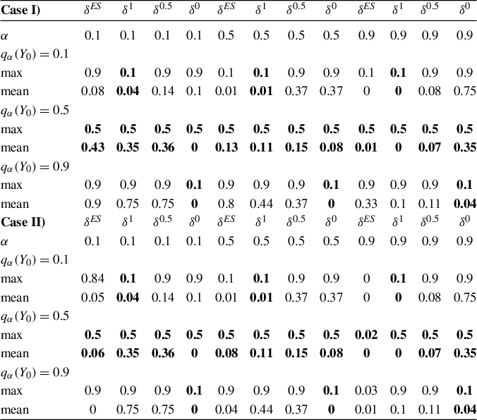

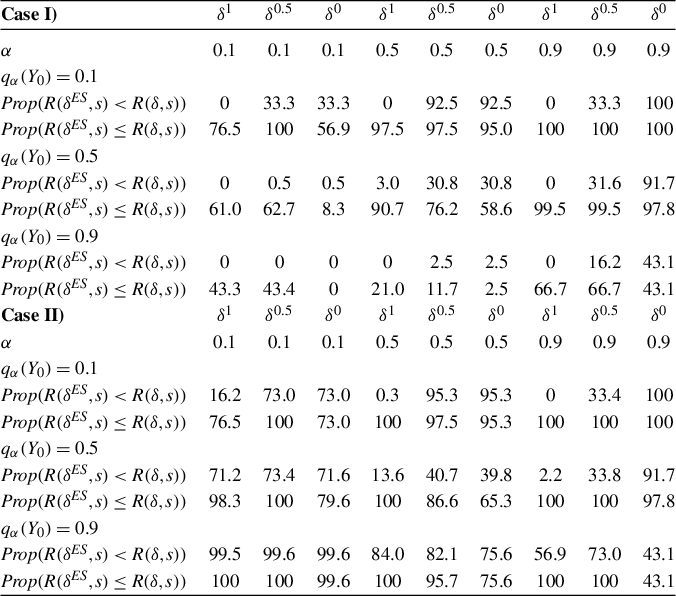


 Open access

