2.1 Experimental set-up

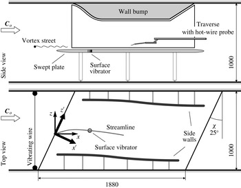
The experiments were conducted in a low-turbulence subsonic wind tunnel T-324 of the Khristianovich Institute of Theoretical and Applied Mechanics (ITAM). The model was mounted in the test section ( $1\times 1\times 4~\text{m}^{3}$ ) at zero angle of attack. The three-dimensional boundary layer of a swept wing was simulated on a swept flat plate having elliptic leading edge. The chordwise pressure gradient was induced by a contoured wall bump (uniform in the spanwise direction) mounted on the test-section ceiling just above the plate. Both the plate and the bump had the same sweep angle ${\it\chi}=25^{\circ }$ . A view from above and a side view of the model are given in figure 1. Similar to experiments of Borodulin et al. (Reference Borodulin, Ivanov, Kachanov, Roschektayev and Fomin2008b , Reference Borodulin, Ivanov, Kachanov and Roschektayev2013) and in contrast to some earlier experiments performed on a similar experimental model (see e.g. Gaponenko, Ivanov & Kachanov Reference Gaponenko, Ivanov and Kachanov1995a ,Reference Gaponenko, Ivanov, Kachanov and Kobayashi b ; Crouch et al. Reference Crouch, Gaponenko, Ivanov and Kachanov1997; Ivanov, Kachanov & Koptsev Reference Ivanov, Kachanov and Koptsev1998, Reference Ivanov, Kachanov and Koptsev2001; Gaponenko et al. Reference Gaponenko, Ivanov, Kachanov and Crouch2002), the present model was modified. Namely, it was equipped with two contoured sidewalls in order to diminish the influence of the wind-tunnel test-section walls and to provide better satisfaction of the sweep condition. Note that the turbulence level ${\it\varepsilon}$ in this wind tunnel at a free-stream velocity of approximately 5– $10~\text{m s}^{-1}$ is usually less than 0.02 % (in the frequency range higher than 1 Hz). However, the contoured wall bump and the sidewalls of the present experimental model described above introduced some additional (low frequency) disturbances into the flow, and the r.m.s. value of ${\it\varepsilon}$ (defined as ${\it\varepsilon}=u^{\prime }/U_{e}$ ) was higher at the conditions of the present experiments – around 0.06 % (over the same frequency range).

Figure 1.

Sketch of experimental model. Dimensions are in mm.

The main coordinate systems used in the present experiments are the following. The $(x,z)$ -system is connected to the incoming free-stream direction (upstream of the model) with the mean velocity vector $\boldsymbol{C}_{o}$ parallel to the $x$ -axis. The $x^{\prime }$ -axis is directed along the chord and starts at the leading edge of the model. The axis $z^{\prime }$ is parallel to the leading edge. The $(x^{\ast },z^{\ast })$ -coordinate system is local and the $x^{\ast }$ -axis is directed along the local mean-velocity vector $\boldsymbol{C}_{e}$ of the potential flow near the external edge of the boundary layer. It is also convenient to use an additional axis $x_{c}$ , which is parallel to the $x$ -axis but has always its origin on the swept-plate leading edge, as well as an additional axis $z_{c}^{\prime }$ , which is like the $z^{\prime }$ -axis but always has its origin at the model centreline, i.e. at  $z=0$ .

All main measurements were carried out by means of the hot-wire anemometer AA Lab Systems AN-1003. Two kinds of measurements were performed: (i) single-wire measurements with which the majority of results were obtained and (ii) double-wire measurements for investigation of the base-flow structure and the free-stream vortex shape.

During the single-wire measurements, the hot-wire probes were made of Wollaston wire with a platinum core of $6~{\rm\mu}\text{m}$ in diameter with the length of the sensitive element at approximately 0.3 mm. The probes were calibrated against a Pitot–Prandtl tube in the incident flow upstream the experimental model. In the case of the double-wire measurements, V-shaped probes with gilded Tungsten wires of $5~{\rm\mu}\text{m}$ in diameter were used. Angular and speed calibrations of these probes were also performed in the free stream far upstream the experimental model. Both kinds of probe are standard for our group, have been used for more than 30 years and are manufactured in the laboratory. In all cases, the calibration curves were approximated by King’s law. The procedure of determining the velocity components based on the double-wire measurements was developed in our group in the 1980s and takes into account possible drift of the hot-wire signals due to wire contamination and flow temperature variations.

The signals used for generation of the free-stream vortices and the surface vibrations, as well as the reference signal, were produced by an 8-channel, computer controlled, electronic unit VS-II. This unit accepted data from the computer and stored them in a RAM. In ‘playback’ mode the clock pulses produced by an external generator went to a counter, which advanced the RAM address bus. The data bus was connected to D/A converters combined with amplifiers (when necessary). The clock frequency was set to 2048 Hz and the length of every signal realization produced by the electronic unit VS-II was equal to $T_{sam}=1$  s. The clock frequency was measured by a frequency meter and kept constant with very high accuracy. Signal produced by channel 1 was used for feeding the loudspeaker connected with the surface vibrator. For example, for frequency of the surface vibrations $f_{sur}=70$  Hz the sinusoidal signal at channel 1 had 70 periods per one realization. Channels 7 and 8 of unit VS-II were used for feeding the stepping motors, which produced oscillations of the wire exciting the free-stream vortices. In the case of excitation of the vortices at frequency $f_{vor}=40$  Hz, sinusoidal signals on channels 7 and 8 had 40 periods per one realization. The output signal from channel 1 of unit VS-II was amplified by a power amplifier to feed the loudspeaker, while the output signals from channels 7 and 8 were connected directly to two stepping motors.

The sampling frequency used for the data acquisition was equal to 1200 Hz. The time-periodic component of the signal was ensemble averaged for 10 signal realizations. As far as the length of every realization was equal to 1 s, this provided an averaging of $N=10f$ periods of the sinusoidal wave with frequency $f$  Hz. For example, for a frequency of 70 Hz, $N$ was equal to 700 periods. The reference signal used for ensemble averaging was also produced by unit VS-II and had frequency $f_{sam}=1/T_{sam}=1$  Hz. In this way every excited signal and every signal measured in the flow (including the combination frequencies such as $f_{CF}=f_{sur}\pm f_{vor}$ ) had an integer number of periods per realization (1 s) if its frequency was equal to an integer number of Hertz. Due to this circumstance the Fourier series rather than Fourier integrals were used during the frequency spectral analysis of the experimental data. Therefore, no spectral windows were applied (or in other words, a rectangular window was always used) because the Fourier series provided us with exact values of the series coefficients in the cases of periodic signals, as in the present experiments.

2.2 Base-flow characteristics

The characteristics of the three-dimensional base-flow field over the present model were measured carefully in both the potential flow and inside the boundary layer, using both single-wire and V-shaped double-wire probes. The experimental model and the base-flow conditions were designed in a way to ensure absence of any significant ‘natural’ (i.e. uncontrolled) boundary-layer perturbations, including stationary CF-instability vortices. In particular, the swept-plate surface was extremely smooth and the used sweep angle and pressure-gradient parameter were not very large, as well as the flow velocities. All conditions provided both weak initial amplitudes of uncontrolled CF-vortices and their weak downstream amplification. Therefore, only controlled non-stationary disturbances were present in the flow and were measured and analysed.

The most important base-flow characteristics are presented below. Additional information is given also in Borodulin et al. (Reference Borodulin, Ivanov, Kachanov and Roschektayev2013).

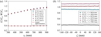
Shown in figure 2(a) are downstream distributions of the chordwise ( $U^{\prime }/C_{o}$ ) and spanwise ( $W^{\prime }/C_{o}$ ) components of the potential flow mean velocity measured just above the boundary-layer edge at a wall-normal distance $y=18$  mm. (Here ( $^{\prime }$ ) denotes the ( $x^{\prime },z^{\prime }$ )-coordinate system.) The data were obtained three times (in different days) in three sets of measurements designated hereafter as sets 1, 2 and 3. The results are presented for $C_{o}=17.7~\text{m s}^{-1}$ . However, it was shown that the potential flow structure is practically independent of the free-stream speed. It is seen that the chordwise velocity component $U^{\prime }/C_{o}$ increases downstream monotonically due to a favourable pressure gradient produced by the wall bump. Meanwhile, the spanwise velocity component $W^{\prime }/C_{o}$ remains practically constant. The solid line in figure 2(a) displays a linear approximation of the experimental points for the $W^{\prime }/C_{o}$ -component. It is seen that the sweep condition $W^{\prime }/C_{o}=\text{const.}$ is satisfied very well in a broad range of variation of the streamwise coordinates, which includes the whole region of the present measurements (between $x_{c}=450$ and 750 mm, approximately).

Figure 2.

Downstream (a, $z=0$ ) and spanwise (b) distributions of chordwise and spanwise components of potential flow mean velocity. $C_{o}=17.7~\text{m s}^{-1}$ , $y=18$  mm.

The satisfaction of the sweep condition is also seen very well in figure 2(b) displaying spanwise distributions of the chordwise ( $U^{\prime }/C_{o}$ ) and spanwise ( $W^{\prime }/C_{o}$ ) components of the potential flow mean velocity measured just above the boundary-layer edge at a wall-normal distance $y=18$  mm for three different chordwise locations. The constancy of both the chordwise and spanwise mean-velocity components displays the spanwise uniformity of the potential flow over the present experimental model.

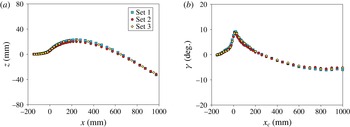
The shape of the potential flow streamline is shown in figure 3(a) in the ( $x,z$ )-plane. Note that the streamwise and spanwise coordinates have significantly different scales in this plot. The downstream distribution of yaw angle of the potential flow mean-velocity vectors is presented in figure 3(b). Maximum deviation of the yaw angle from the zero value is seen to be approximately $+10^{\circ }$ near the swept-plate leading edge and about $-6^{\circ }$ in the end of the studied region.

Figure 3.

Shape of potential flow streamline (a) and downstream distribution of potential flow yaw angle (b). $C_{o}=17.7~\text{m s}^{-1}$ , $y=18$  mm,  $z=0$ .

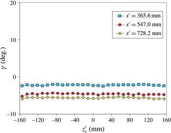
The spanwise uniformity of yaw angles of the potential flow mean-velocity vectors is demonstrated in figure 4 for three chordwise positions. Thus, the measurements illustrated above (in figures 2 a,b, 4) have shown that the potential base flow under study corresponds (excluding the wall curvature effects) to a flow over an infinite span 25° swept wing at its initial section, where the flow accelerates.

Figure 4.

Spanwise distributions of yaw angle of potential flow mean-velocity vectors measured for three chordwise positions. $C_{o}=17.7~\text{m s}^{-1}$ , $y=18$  mm.

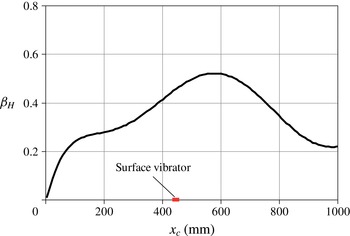
The streamwise distribution of the experimentally obtained Hartree parameter is presented in figure 5. This parameter was estimated according to formulas:

where $U_{e}^{\prime }$ is the flow velocity at the boundary-layer edge.

Figure 5.

Streamwise distribution of Hartree parameter ${\it\beta}_{H}$ estimated based on experimental data.

Figure 6.

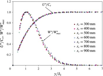
Wall-normal profiles of normalized streamwise ( $U^{\ast }/C_{e}$ ) and cross-flow ( $W^{\ast }/W_{max}^{\ast }$ ) components of mean-velocity vectors measured for various downstream positions. $C_{o}=17.7~\text{m s}^{-1}$ , $z=0$ .

Figure 7.

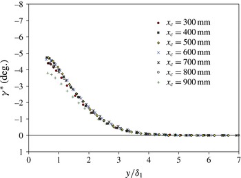
Wall-normal profiles of yaw angle of mean-velocity vectors measured for various downstream positions. $C_{o}=17.7~\text{m s}^{-1}$ , $z=0$ .

Figure 8.

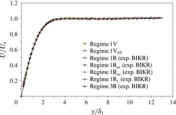
Wall-normal profiles of streamwise velocity component measured at $x_{c}=523.5$  mm,  $z=0$ in several regimes of receptivity measurements in the presence of free-stream vortices. Abbreviation BIKR indicates measurements performed in regimes studied by Borodulin et al. (Reference Borodulin, Ivanov, Kachanov and Roschektayev2013).

Because of a typical accuracy problem appearing at differentiation of the experimental data, the experimental $U^{\prime }(x^{\prime })$ -distributions were first smoothed by natural cubic-spline functions. After that, the values of the Hartree parameter were determined for several sets of measurements and averaged. The repeatability of the experimental points was reasonably good with scatter of approximately $\pm 0.02$ , i.e. approximately 4 % of the maximum value of  ${\it\beta}_{H}$ .

Note that at the surface vibrator centre position ( $x_{c}=x_{cv}=446.0$  mm, $x^{\prime }=x_{v}^{\prime }=404.2$  mm, $z=0$ ), the Hartree parameter has a value of 0.457, while the boundary-layer edge velocity is $U_{ev}=6.50~\text{m s}^{-1}$ .

Shown in figure 6 are two sets of wall-normal profiles of the streamwise ( $U^{\ast }/C_{e}$ ) and spanwise ( $W^{\ast }/W_{max}^{\ast }$ , the cross-flow profile itself) components of mean-velocity vectors versus the dimensionless coordinate $y/{\it\delta}_{1}$ , measured for various streamwise positions in the local ( $x^{\ast },z^{\ast }$ )-coordinate system (i.e. in the system having the $x^{\ast }$ -axis parallel to the free-stream mean-velocity vector at the boundary-layer edge). It is seen that for a broad range of variation of the streamwise coordinate, the shape of the streamwise velocity profiles remain almost the same. The shape of the cross-flow profiles also change very little. It is found also that both the shape of the wall-normal profiles and the cross-flow magnitude are practically independent of the spanwise coordinate $z^{\prime }$ (at least in the studied range between $z_{c}^{\prime }=-110.3$ and $+110.3$  mm).

The wall-normal distributions of the velocity-vectors’ yaw angles are illustrated in figure 7. The maximum measured angles are of approximately 5°, but they can reach values of about 7° in the very vicinity of the wall (where the double-wire measurements are difficult to perform).

It was expected that the presence of the source of weak free-stream vortices (i.e. the vibrating wire) would be able to perturb the base flow, at least slightly. Therefore, additional boundary-layer measurements were performed at particular conditions of the present receptivity experiments described in § 2.5 and similar experiments (Borodulin et al. Reference Borodulin, Ivanov, Kachanov and Roschektayev2013) performed in presence of a phased roughness. A set of wall-normal profiles of the $x$ -component of mean-flow velocity shown in figure 8 is measured at $x_{c}=523.5$  mm, $z=0$ in different sets of receptivity experiments (both present ones and those of Borodulin et al. (Reference Borodulin, Ivanov, Kachanov and Roschektayev2013)) with approximately the same wall-normal position of the free-stream vortex street. The profiles are in quite good agreement with the those measured in the absence of the free-stream vortex generator. It is also seen that all profiles coincide with each other, showing a very good repeatability of the experimental data. A very minor influence of the vortex generator on the potential flow may be seen as a week velocity deficit in the range $y/{\it\delta}_{1}=4{-}12$ . A maximum value of this deficit (reached at the vortex street centre) is less approximately 0.5 %. No influence of the vortex generator on the mean flow inside the boundary layer is found.

It is found that at the position of the surface vibrator, the average value of the boundary-layer displacement thickness ${\it\delta}_{1}$ is ${\it\delta}_{1v}=1.23$  mm and the corresponding local Reynolds number $Re_{v}=U_{ev}{\it\delta}_{1v}/{\it\nu}=496\pm 8$ (the scattering is explained by changing the atmospheric parameters on the different days of measurement). The accuracy of the measurements of ${\it\delta}_{1}$ was estimated as $\pm 0.015$  mm.

A more detailed description of the boundary-layer characteristics is presented by Borodulin et al. (Reference Borodulin, Ivanov, Kachanov and Roschektayev2013).

Note that the boundary-layer characteristics measured on a similar experimental model were compared with Crouch’s calculations by Crouch et al. (Reference Crouch, Gaponenko, Ivanov and Kachanov1998), Gaponenko et al. (Reference Gaponenko, Ivanov, Kachanov and Crouch2002). A very good agreement was found for the wall-normal profiles of the streamwise and spanwise mean-velocity components and of the yaw angles of the mean-velocity vector. Comparison of measured amplitude and phase parts of the CF-mode eigenfunctions with calculations performed based on the linear stability theory was carried out by Crouch et al. (Reference Crouch, Gaponenko, Ivanov and Kachanov1998). Other stability characteristics were compared in detail by Borodulin et al. (Reference Borodulin, Gaponenko, Ivanov, Kachanov, Crouch and Rudyak2000) including distributions of: (i) amplification rates, (ii) streamwise wavenumbers, and (iii) two kinds of phase velocities versus the disturbance frequency, spanwise wavenumber and wave propagation angle. In all cases the agreement turned out to be very good and demonstrated that the disturbances exciting and propagating in the boundary layer of the used experimental model correspond to traveling CF-instability modes.

2.3 Generation of controlled free-stream vortices

For excitation of unsteady free-stream vortices a special generator was used (see Borodulin et al. Reference Borodulin, Ivanov, Kachanov and Roschektayev2013, for more detail). The generator consisted of two electromechanical shakers which held the ends of a thin tungsten wire (of $200~{\rm\mu}\text{m}$ in diameter) under tension. The wire diameter was selected as a compromise between absence of uncontrolled von Kármán vortex street (which appeared at larger wire diameters), linearity of the receptivity mechanism under study and appropriate accuracy of the receptivity measurements. The shakers forced the wire to oscillate in the flow-normal direction with a necessary frequency and amplitude. The shakers were controlled by the signal generator VS-II mentioned above. The free-stream vortex generator was positioned in the wind-tunnel test section in front of the swept-wing model (as shown in figure 1). The vibrating wire was installed perpendicular to the incoming flow direction (i.e. to the vector $\boldsymbol{C}_{o}$ ) at a distance to the swept-plate leading edge $x_{c}=-300$  mm at $z=0$ . The inclination angle of the wire in the ( $z,y$ )-plane, as well as the value of the $y$ -coordinate, were adjusted during the experiment to provide further downstream the parallelism of the vortex axes to the swept-plate surface and the required vortex offset parameter. The vibrating wire excited in the free stream an anti-symmetric array of vortices similar to the well-known von Kármán vortex street but with very small intensity of the vortices.

There were two kinds of measurements aimed to clarify the main properties of the excited vortex streets in the wall-normal direction: (i) single-wire measurements of wall-normal profiles of the streamwise velocity component performed inside and outside the boundary layer and (ii) double-wire measurements of wall-normal profiles of both $u$ - and $v$ -components of the velocity fluctuations outside the boundary layer and at its external edge. The wall-normal disturbance profiles were taken at the exact position of the surface vibrator centre ( $x_{cv}=446$  mm, $z=0$ ). 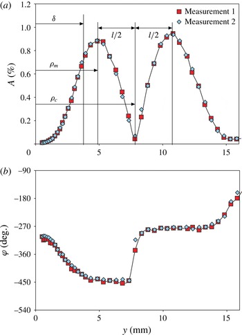Two of them are illustrated in figure 9(a,b) for regime 1V ( $f_{vor}=40$  Hz). 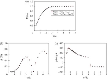Shown there are the amplitude (figure 9 a) and phase (figure 9 b) profiles of the streamwise component of the flow-velocity-fluctuations in the vortex street. The corresponding boundary-layer thickness is also shown in figure 9(a) along with the used vortex offset parameters ${\it\rho}_{m}$ and ${\it\rho}_{c}$ . Almost complete coincidence of the profiles obtained just prior to the main receptivity measurements (measurement 1) and just after them (measurement 2) indicates a very good accuracy and repeatability of the present data.

Figure 9.

Wall-normal profiles of free-stream vortex amplitudes (a) and phases (b) measured in regime 1V over the surface vibrator centre. (a,b) $x_{c}=446~\text{mm}$ , $z=0$ .

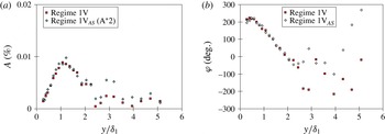
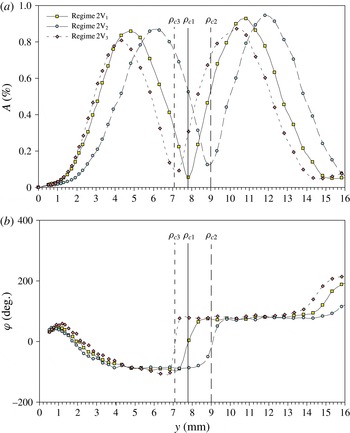
It is seen in figure 9(a,b) that the vortex disturbance has two amplitude maxima, the oscillations of which have opposite phase. The distance $l/2$ in the wall-normal direction between the vortex-street minimum and maximum characterizes the vortex-street width. The inner maximum is positioned near the boundary-layer edge, while the amplitude minimum (i.e. the vortex street centre) and the outer maximum are rather far away from the boundary-layer edge. Figure 9(a,b) shows also that there is no evidence of presence of a cross-flow instability wave with vortex frequency $f_{vor}$ inside the boundary layer at the surface vibrator location.

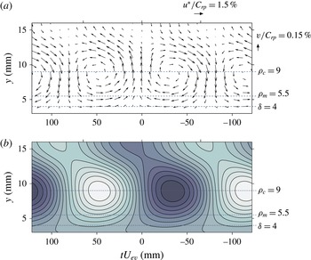
An illustration of one of the results of the double-wire measurements of the velocity disturbance vectors which occurred within the excited vortex street is presented in figure 10(a) in the ( $-t,y$ )-plane ( $f_{vor}=40.0$  Hz, vortex offset parameters ${\it\rho}_{c}=9.0$  mm). The time axis is multiplied by the local potential flow velocity $U_{ev}=6.5~\text{mm ms}^{-1}$ ( $6.5~\text{m s}^{-1}$ ) and has therefore the dimension in millimetres. Such normalization helps to estimate the streamwise wavelength of the free-stream vortices, the speed of propagation of which is close to the local potential flow velocity (see below). The corresponding streamlines are shown in figure 10(b). It is seen that the vortex street under study represents a set of counter-rotating vortices aligned in a row. The axes of all vortices are positioned at $y={\it\rho}_{c}$ . This kind of vortex street is a little bit different from the classic von Kármán vortex street, in which the vortices are displaced from the street centre in a staggered way. Qualitatively similar results were obtained in all other regimes studied.

Figure 10.

Instantaneous shape of free-stream vortex street measured by double-wire probe. The velocity disturbance vector field in the ( $-t,y$ )-plane (a) and the corresponding streamlines (b). (a,b) Regime: W2 (double-wire measurements).

There were several measurements of the distributions of the streamwise velocity component of the vortex perturbations outside the boundary layer in the spanwise and streamwise directions over the surface non-uniformity. These measurements were carried out at a distance to the wall that corresponded to the inner amplitude maximum of the vortex street (see figure 9 a). The obtained results gave us information about a degree of uniformity of the vortex street in the spanwise and streamwise directions, as well as about the orientation of the vortex axes in the ( $x^{\prime },z^{\prime }$ )-plane (i.e. about the streamwise and spanwise wavenumbers of the vortex perturbation). Main results of these measurements are presented below in figure 11.

Figure 11.

Spanwise (a,c) and streamwise (b,d) distributions of velocity disturbance amplitudes and phases within vortex street measured at $y={\it\rho}_{m}=4.85$  mm and $f_{vor}=40.0$  Hz. Experimental points are approximated by straight lines (a,c,d) and exponent (b). Regime 1V. (a,c) $x_{c}=446~\text{mm}$ , (b,d) $z=0$ , (a–d) $y={\it\rho}_{m}=\text{const.}$ ; (a)  $A=0.0005z+0.9048$ , (b) $A=1.6393\text{e}^{-0.0013x_{c}}$ , (c) ${\it\varphi}=0.062z+955.665$ , (d) ${\it\varphi}=2.2996x_{c}-930.59$ .

These measurements were performed in a regime with the most typical free-stream vortex configuration (which corresponds to regimes 1V, 2V, 3V, $2\text{V}_{1}$ and $1\text{V}_{AS}$ as described below in § 2.6). The spanwise (in the $z$ -direction) distributions of the disturbance amplitudes and phases in the vortex street are shown in figure 11(a,c). The measurements are performed at a constant distance to the wall $y={\it\rho}_{m}=4.85$  mm and at the vortex frequency $f_{vor}=40.0$  Hz. The corresponding streamwise (in the $x$ -direction) distributions are presented in figure 11(b,d). Curves in these figures represent the approximation of the experimental points with straight lines (in figure 11 a,c,d) and with an exponent (in figure 11 b).

It is seen from figure 11(a) that the vortex amplitude remains constant in the $z$ -direction with a very high accuracy, demonstrating the spanwise uniformity of the generated vortex street. The phase distribution in figure 11(c) shows that the vortex axis is almost parallel to the $z$ -axis which is consistent with the position of the vibration wire (see figure 1). However, due to the absence of symmetry at such an orientation of the wire, the vortex axis is turning slightly in the ( $x,z$ )-plane. As a result, the value of the spanwise wavenumber ${\it\beta}_{vor}$ is small but finite and equal to $0.062^{\circ }~\text{mm}^{-1}$ or $0.00108~\text{rad mm}^{-1}$ (see the approximation formula in the caption of figure 11 c).

In the streamwise direction the vortex amplitude decreases slowly (figure 11 b) in an exponential way due to viscose forces with negative increment $-{\it\alpha}_{i}=-0.0013~\text{mm}^{-1}$ . (It is necessary also to keep in mind that the inner maximum of the vortex street is rather close to the boundary-layer edge and probably interacts with it.) The phase distribution in figure 11(d) shows that the vortices propagate downstream with a certain speed $C_{x\,vor}$ , which can be estimated from the streamwise wavenumber ${\it\alpha}_{r\,vor}=2.30^{\circ }~\text{mm}^{-1}=0.0401~\text{rad mm}^{-1}$ (see the approximation formula in the caption of figure 11 d). Indeed, $C_{x\,vor}=360f_{vor}/{\it\alpha}_{r\,vor}=6.26~\text{m s}^{-1}$ , while the edge velocity over the vibrator is $U_{ev}=6.50~\text{m s}^{-1}$ . This means that the non-dimensional speed of the vortex street in the $x$ -direction is $C_{x\,vor}/U_{ev}=0.96$ , which is very close to unity, i.e. the vortices propagate almost with the free-stream speed. This speed corresponds to that characteristic for the low-amplitude vortex street propagating in the free-stream.

The inclination angle of the vortex axis to the $z$ -axis can be determined as ${\it\theta}_{vor}=\tan ^{-1}({\it\beta}_{vor}/{\it\alpha}_{r\,vor})=1.5^{\circ }$ . In the coordinate systems ( $x^{\prime },z^{\prime }$ ) and ( $x^{\ast },z^{\ast }$ ) this angle is ${\it\theta}_{vor}^{\prime }={\it\theta}_{vor}+{\it\chi}=26.5^{\circ }$ and ${\it\theta}_{vor}^{\ast }={\it\theta}_{vor}-{\it\gamma}_{e}=1.5+2.8=4.2^{\circ }$ , respectively, because at the position of the vibrator ( $x_{c}=446$  mm) the local yaw angle of the potential flow ${\it\gamma}_{e}=-2.8^{\circ }$ (see figure 3 b). In the ( $x^{\prime },z^{\prime }$ )-coordinate system, the streamwise wavenumber ${\it\alpha}_{r\,vor}^{\prime }=2.059^{\circ }~\text{mm}^{-1}=0.0359~\text{rad mm}^{-1}$ and the spanwise wavenumber ${\it\beta}_{vor}^{\prime }=1.027^{\circ }~\text{mm}^{-1}$ or $0.0179~\text{rad mm}^{-1}$ .

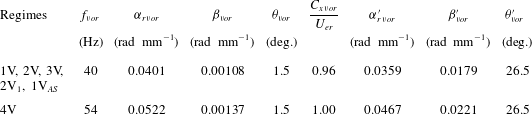
All main parameters of the free-stream vortex street measured in the vicinity of the surface vibrator are given in table 1.

Table 1.

Main parameters of free-stream vortices.

2.4 Generation of controlled surface vibrations

For modelling surface vibrations we used a special device – a surface vibrator, which was mounted at the centreline of the swept plate ( $z=0$ ) flush with the wall at a distance $x_{c}=446$  mm from the leading edge (see also figure 5). This location was selected near the estimated beginning of the region of significant CF-instability and, hence, of amplification of the most important CF-modes under study. Simultaneously this location corresponded to the region where the cross-flow itself has been formed due to growth of the Hartree parameter (see figure 5).

The vibrator consisted of a hollow cylindrical insert on the top of which a thin (0.9 mm) rubber membrane with diameter of 10 mm was glued. This diameter provided excitation of a broad wavenumber spectrum of surface vibrations discussed in § 3.4. The time-periodic membrane oscillations were driven by pressure fluctuations produced in a sealed cavity under the membrane. These fluctuations were created by a powerful loudspeaker placed outside the wind tunnel and connected with the vibrator by means of plastic pipe. The amplitude and frequency of the membrane oscillations were controlled by operating with electric signal feeding the loudspeaker. No uncontrolled oscillations excited by the flow were observed at the experimental conditions.

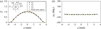
The shape of the membrane oscillation (i.e. the spatial distributions of the oscillation amplitude and phase) was measured by means of a non-contact optical displacement measuring system OptoNCDT 1605 (Micro-Epsilon Messtechnik) with a laser sensor LD 1605-2. The main results of the measurements are presented in figure 12 where normalized amplitudes (figure 12 a) and phases (figure 12 b) of the vibrations are shown as functions of the distance ${\it\rho}$ from the centre of the vibrator. The normalized oscillation amplitude $a_{m}=A_{m}/A_{mo}$ , where $A_{m}$ is the dimensional amplitude and $A_{mo}$ is the dimensional amplitude in the centre of the membrane (i.e. at ${\it\rho}=0$ ). These results are obtained for the frequency of vibrations $f_{sur}=70$  Hz used in regimes 1V and 4V. It is seen that the shape of the oscillations is very axisymmetric and is very well approximated by a symmetrical eighth-order polynomial as shown in the caption of figure 12(a). The oscillation phase distributions (figure 12 b) demonstrate almost perfect flatness over the whole membrane surface. This means that the shape of the membrane deflection is the same at any time instant and corresponds to that shown in figure 12(a). This shape is also shown to be independent of both the vibration frequency and amplitude.

Figure 12.

Normalized amplitudes (a) and phases (b) of surface vibrations measured over the vibrator along four different lines shown in the insert in (a). (a)  $a_{m}=1.9683\times 10^{-6}{\it\rho}^{8}-8.607\times 10^{-5}{\it\rho}^{6}+0.00115803{\it\rho}^{4}-0.0441729{\it\rho}^{2}+1.0000332$ .

The maximum (at ${\it\rho}=0$ ) zero-to-peak vibration amplitudes were found in regimes 1V, 2V, 3V, 4V, $2\text{V}_{1}$ , $2\text{V}_{2}$ and $2\text{V}_{3}$ to be equal to: $A_{mo}=410$ (corresponds to $A_{sur1}$ in table 2), 343 (corresponds to $A_{sur2}$ ), 379 (corresponds to $A_{sur3}$ ), 400 (corresponds to $A_{sur4}$ ), 346, 346 and $346~{\rm\mu}\text{m}$ (correspond to $A_{sur5}$ in table 2), respectively. The results of measurements of the membrane oscillations will be used for subsequent Fourier decomposition and determination of the vibration-vortex receptivity coefficients.

Table 2.

Most important regimes of receptivity measurements.

The phase of the membrane oscillations needed for finding the receptivity coefficients must be measured by the same hot-wire system as the phases of all flow-velocity perturbations and must be counted with respect to the same reference signal. Only in this case, the measured phase of the membrane oscillations can be comparable with all other measured phases (of both the free-stream vortices and the excited instability waves). In order to find this phase, wall-normal profiles were measured in every regime just above the centre of the oscillating membrane. The phase profiles were extrapolated onto the membrane surface and an assumption was used that the phase of the flow-velocity oscillations measured very near the wall corresponded to the inverted phase of the surface oscillations. Such a procedure for determination of the vibration phase was used successfully in several previous experiments on vibration receptivity in three- and two-dimensional boundary layers and displayed, in particular, a very good agreement with several receptivity theories (see e.g. Ivanov, Kachanov & Obolentseva Reference Ivanov, Kachanov and Obolentseva1999; Bake et al. Reference Bake, Ivanov, Fernholz, Neemann and Kachanov2002b ; Gaponenko et al. Reference Gaponenko, Ivanov, Kachanov and Crouch2002; Kachanov, Koptsev & Smorodsky Reference Kachanov, Koptsev and Smorodsky2002).

2.5 Regimes and procedures of measurements

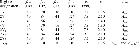
The receptivity measurement campaign included eight main regimes with different disturbance parameters presented in table 2.

The following four values were measured in every regime in each spatial point by means of a single-wire probe of the hot-wire anemometer: (i) the mean flow velocity, (ii) the r.m.s. amplitude, (iii) the phase of the velocity disturbance at one of studied frequencies and (iv) the r.m.s. intensity of the total velocity fluctuations. Besides that, the ensemble-averaged time-trace was recorded at every spatial point in all regimes when the spectrum contained more than one frequency harmonic under investigation. These time-traces were subjected to temporal spectral decomposition by means of Fourier series to obtain the amplitudes and phases of all other spectral components of interest. The single-wire probe measured the $x$ -components of both the mean flow-velocity vector and the vector of velocity fluctuations. In the cases of double-wire measurements, the same four main quantities (listed above as i, ii, iii and iv) were measured in every spatial point for each wire of the probe.

Selection of surface ( $f_{sur}$ ) and vortex ( $f_{vor}$ ) frequencies was conditioned by some requirements for the generated combination modes, the difference modes CF1, first of all. In real practical situations, the frequencies $f_{sur}$ and $f_{vor}$ can be very different (often rather high), while the vibration-vortex receptivity mechanism is able to redistribute the disturbance energy in the frequency spectrum and to provide, in particular, excitation of CF-modes having most dangerous frequencies for the cross-flow instability mechanism. Therefore, the excited boundary-layer perturbations were close to either amplified, neutral or weakly attenuating CF-modes depending on the particular value of the spanwise wavenumber (we have studied many of them for every frequency).

Four investigated regimes (1V, 2V, 3V and 4V) corresponded to different frequencies of the surface vibrator ( $f_{sur}$ ) and free-stream vortex ( $f_{vor}$ ) and provided various values of the frequency ratio $k=f_{sur}/f_{vor}$ . The excitation of the cross-flow wave was mainly observed in these regimes at the difference combination frequency $f_{CF1}=f_{sur}-f_{vor}$ . However, a small peak at the sum combination frequency $f_{CF2}=f_{sur}+f_{vor}$ was also observed in the spectrum in the most of cases and was measured. Its amplitude was much lower, and the accuracy of its measurements significantly worse. The vortex-street centre offset ${\it\rho}_{c}$ and the vortex-street maximum offset ${\it\rho}_{m}$ (see below) were approximately the same in these regimes and equal to 7.8 and 4.85 mm, respectively. The examined dimensional frequencies $f$ correspond to the frequency parameters $F=F_{1}f$ where $F_{1}=2{\rm\pi}{\it\nu}/U_{ev}^{2}=2.36\times 10^{-6}$ is the unit frequency parameter.

Note that in regimes 3V and 4V the cross-flow waves excited at $f_{CF1}$ had the same frequencies of 16.0 Hz, although the vortex and vibration frequencies were different. Similarly, in regimes 2V and 4V the cross-flow waves excited at $f_{CF2}$ had the same frequencies of 124.0 Hz, although frequencies $f_{sur}$ and $f_{vor}$ were again different. These regimes were specifically chosen in this way in order to have the possibility of investigating the dependence of the receptivity characteristics on the frequency ratio $k=f_{sur}/f_{vor}$ , which can be called the parameter of vibrational non-stationarity. For example, the case when $k$ is close to zero would correspond to a quasi-stationary vibrator and $k>1$ corresponds to essentially non-stationary vibrations (as in all cases studied in the present experiments).

In the three regimes $2\text{V}_{1}$ , $2\text{V}_{2}$ and $2\text{V}_{3}$ the vortex-street centre offset ${\it\rho}_{c}$ was varied, while the frequencies were the same as in regime 2V. During this variation the swing of the wire oscillation was kept constant (about 7.5 mm). To check the linearity of the receptivity problem with respect to the vibration amplitude some additional measurements were also carried out in regime  $1\text{V}_{AS}$ , which were similar to regime 1V. In regime  $1\text{V}_{AS}$ one spanwise distribution (at $x^{\prime }=501.6$  mm or $x_{c}=553.5$  mm, $U/U_{e}\approx 0.6$ , $y=\text{const.}$ ) and one wall-normal profile (at $x^{\prime }=501.6$  mm or $x_{c}=553.5$  mm, $z=0$ ) were measured at two amplitudes of vibration. Every pair of measurements was made during a single scan in space with switching of the vibrator input voltage from one value to another at every spatial point. This method provided the highest accuracy for the measurements.

There were also two kinds of additional measurements, which were performed for the conditions of regimes 1V, 2V, 3V and $2\text{V}_{1}$ . In the first kind of measurement, the orientation of the vortex street and its uniformity in space were calibrated outside the boundary layer. The main results of these measurements are presented in § 2.3. In the second kind of experiment, some special measurements were performed for detection the presence of any cross-flow waves exited in an uncontrollable way upstream of the vibrator. These measurements included a wall-normal profile at the chordwise position of the vibrator (but at the side of it, at $x_{c}=446.0$  mm, $z=30$  mm) and two streamwise distributions (at $z=30$  mm) inside (at $U/U_{e}\approx 0.6$ , $y=\text{const.}$ ) and outside of (at $y={\it\rho}_{m}$ ) the boundary layer.

In addition, there were three main regimes of the double-wire probe measurements of the $u$ - and $v$ -components of the velocity-fluctuation vector inside the free-stream vortex street. The measurements of the wall-normal profiles were performed over the centre of the surface vibrator ( $x_{c}=446.0$  mm, $z=0$ ) for a fixed vortex frequency $f_{vor}=40.0$  Hz and vortex offset parameters ${\it\rho}_{c}=7.8$ , 9.0 and 7.1 mm. These three double-wire regimes correspond to the free-stream vortex conditions of main regimes: (i) 1V, 2V, 3V, $2\text{V}_{1}$ and $1\text{V}_{AS}$ , (ii)  $2\text{V}_{2}$ and (iii)  $2\text{V}_{3}$ . Some of results of these measurements are illustrated in § 2.3.

2.6 Spectral modes participating in the receptivity mechanism

As was shown above (see table 1), the free-stream vortex street represents a single Fourier mode of the frequency-spanwise-wavenumber spectrum with a fixed frequency ${\it\omega}_{vor}=2{\rm\pi}f_{vor}$ , spanwise wavenumber ${\it\beta}_{vor}^{\prime }$ and streamwise wavenumber ${\it\alpha}_{r\,vor}^{\prime }$ . This mode can be designated by the vector ( ${\it\omega}_{vor},{\it\beta}_{vor}^{\prime },{\it\alpha}_{r\,vor}^{\prime }$ ). Meanwhile, the corresponding spectrum of the surface vibrations consists of an infinite number of mode-vectors ( ${\it\omega}_{sur},{\it\beta}_{sur}^{\prime },{\it\alpha}_{r\,sur}^{\prime }$ ) with the same frequency ${\it\omega}_{sur}$ but various values of ${\it\beta}_{sur}^{\prime }$ and different values of ${\it\alpha}_{r\,sur}^{\prime }$ for every value of ${\it\beta}_{sur}^{\prime }$ (see section below). In the ‘linear’ receptivity problem (in which the receptivity coefficients defined below are independent of the two disturbance amplitudes), the scattering of the free-stream vortices on the localized surface vibrations leads to excitation of the combination cross-flow modes CF1 and CF2, which correspond in Fourier space to vectors ( ${\it\omega}_{CF1},{\it\beta}_{CF1}^{\prime },{\it\alpha}_{r\,CF1}^{\prime }$ ) and ( ${\it\omega}_{CF2},{\it\beta}_{CF2}^{\prime },{\it\alpha}_{r\,CF2}^{\prime }$ ), respectively. Similar to the vector of vibrations, the frequency of each of these combination modes ${\it\omega}_{CFi}$ ( $i=1,2$ ) is fixed and the spanwise wavenumber ${\it\beta}_{CFi}^{\prime }$ corresponds to the broadband spectrum. However, the streamwise wavenumber ${\it\alpha}_{r\,CFi}^{\prime }$ is not a free variable but a function of ${\it\beta}_{CFi}^{\prime }$ corresponding to the dispersion curve

for the CF-instability waves with the given frequency ${\it\omega}_{CFi}$ found experimentally for the chordwise position of the surface vibrator centre. The frequencies and the wavenumbers of the excited combination CF-modes are determined from the relationships:

where ${\it\beta}_{sur1}^{\prime }$ , ${\it\beta}_{sur2}^{\prime }$ and ${\it\alpha}_{r\,sur1}^{\prime }$ , ${\it\alpha}_{r\,sur2}^{\prime }$ are the spanwise and streamwise wavenumbers, respectively, of the resonant components in the surface vibration spectra. Taking into account (2.2) the resonant wavenumbers in the spectrum of vibrations can be found in experiment from (2.3) as

Thus, during the experimental data processing, the components of the combination vectors and the resonant components of the vector of vibrational spectrum can be determined in the following way. The values of the combination frequencies can be found from (2.3) as just two numbers. Then, the results of measurements in the boundary layer give us two broadband spanwise wavenumber spectra of the CF-modes CF1 and CF2 excited at combination frequencies (see figures 15 and 16 in § 3.2), as well as the values of the streamwise wavenumbers $\tilde{{\it\alpha}}_{r\,CF1}^{\prime }=\tilde{{\it\alpha}}_{r\,CF1}^{\prime }({\it\omega}_{CF1},{\it\beta}_{CF1}^{\prime })$ and $\tilde{{\it\alpha}}_{r\,CF2}^{\prime }=\tilde{{\it\alpha}}_{r\,CF2}^{\prime }({\it\omega}_{CF2},{\it\beta}_{CF2}^{\prime })$ .

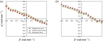
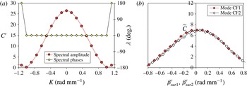
Next, the resonant spanwise and streamwise wavenumbers of the spectrum of vibrations can be determined from (2.4). An example of the resulting dispersion and resonant curves obtained for waves CF1 and CF2 are presented in figure 13(a,b), respectively, for regime 2V. The corresponding points for the free-stream vortex wavevectors are also shown in these figures with triangles. The dispersion curves are mainly consistent with those found in previous CF-stability experiments (see e.g. Gaponenko et al. Reference Gaponenko, Ivanov and Kachanov1995a ,Reference Gaponenko, Ivanov, Kachanov and Kobayashi b ) and linear CF-stability calculations Borodulin et al. (Reference Borodulin, Gaponenko, Ivanov, Kachanov, Crouch and Rudyak2000). These resonant curves were used to obtain the resonant spectra of vibrations discussed below (§ 3.4).

Figure 13.

Example of dispersion and resonant curves obtained for modes CF1 (a) and CF2 (b) in regime 2V.

3.1 CF-wave trains excited by free-stream vortices on surface vibrations

Special detailed measurements performed inside the boundary layer have shown clearly (not illustrated here) that in the present experiments, the free-stream vortex street does not excite in the boundary layer any instability waves in the region upstream the controlled surface vibrations. This means that all CF-waves observed downstream of the surface vibrator are excited only due to the interaction of the free-stream vortices with these vibrations.

Other special detailed measurements have shown that the receptivity (and instability) mechanisms under study are linear at the present experimental conditions (see § 4). By the linearity of the corresponding receptivity mechanisms we assume that the corresponding receptivity coefficients are independent of amplitudes of the two external perturbations (i.e. both the free-stream vortices and the surface non-uniformities). This property was checked via demonstration of the independence of the wall normal and spanwise distributions of phases and the scaled amplitudes of the excited CF-waves from the amplitudes of both surface vibrations and free-stream vortices.

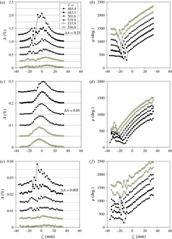
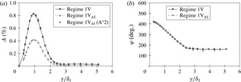
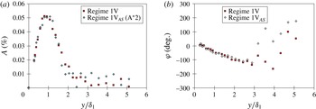
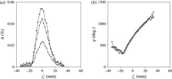
Shown in figure 14(a–f) are three of the four pairs of plots belonging only to one set (of 20 studied) of the spanwise distributions of the boundary-layer disturbance amplitudes and phases. This set is obtained in regime 2V for frequency spectrum modes with frequencies: (i) of surface vibrations $f_{sur}=84$  Hz (figure 14 a,b), (ii) of CF1 combination mode $f_{CF1}=f_{sur}-f_{vor}=44$  Hz (figure 14 c,d) and (iii) of CF2 combination mode $f_{CF2}=f_{sur}+f_{vor}=124$  Hz (figure 14 e,f). The measurements are performed at $U/U_{e}\approx 0.6$ ( $y=\text{const.}$ ), i.e. approximately at the amplitude maximum of the excited cross-flow waves (Gaponenko et al. Reference Gaponenko, Ivanov, Kachanov and Crouch2002). It is seen that the perturbations represent a wave train that is qualitatively similar to those usually observed in previous experiments devoted to the vibration and roughness receptivity (studied e.g. by Gaponenko et al. Reference Gaponenko, Ivanov, Kachanov and Crouch2002). The maximum amplitudes of the excited combination modes CF1 and CF2 (figure 14 c,e) are about 0.050 % and 0.013 %, respectively. They decay downstream; the corresponding phases grow in contrast (figure 14 d,f). The CF-waves excited at the frequency of the surface vibrations have significantly higher maximum amplitudes reaching approximately 0.8 % in the beginning of the region of main measurements (figure 14 a).

Figure 14.

Typical set of spanwise distributions of the boundary-layer disturbance amplitudes (a,c,e) and phases (b,d,f) obtained in regime 2V at $U/U_{e}\approx 0.6$ ( $y=\text{const.}$ ) at surface vibration frequency $f_{sur}=84$  Hz (a,b) and at frequencies of modes CF1 $f_{CF1}=44$  Hz (c,d) and CF2 $f_{CF2}=124$  Hz (e,f). Every amplitude curve is shifted from with respect to its neighbour by ${\rm\Delta}A$ indicated in plot.

The distributions measured in regimes 1V, 3V and 4V (not shown) are qualitatively similar to those obtained in regime 2V. However, quantitative differences are quite significant and depend on the frequency of the excited mode and seem to depend on the regime of their excitation. The spanwise distributions obtained in regimes  $2\text{V}_{1}$ , $2\text{V}_{2}$ and $2\text{V}_{3}$ display reduction of the excited CF-wave amplitudes with an increase of the vortex offset parameter ${\it\rho}_{c}$ from 7.1 mm through 7.8 mm until 9.0 mm (not shown). The amplitudes of the cross-flow wave CF1 correlate very well with the vortex amplitudes measured at the boundary-layer edge. They both decrease when ${\it\rho}_{c}$ increases. Meanwhile, the phase distributions of the excited combination CF-modes display their independence of the vortex offset parameter (not shown).

Figure 15.

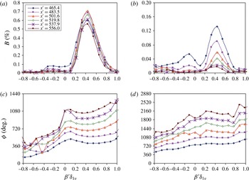
Amplitude (a,b) and phase (c,d) parts of spanwise-wavenumber spectra of modes CF1 (a,c) and CF2 (b,d) of boundary-layer disturbances excited by the vibration-vortex receptivity mechanism in regime 1V. $U/U_{e}\approx 0.6$ , $y=\text{const}$ . (a,c) $f=30$  Hz, (b,d) $f=110$  Hz.

Figure 16.

Amplitude (a,b) and phase (c,d) parts of spanwise-wavenumber spectra of modes CF1 (a,c) and CF2 (b,d) of boundary-layer disturbances excited by the vibration-vortex receptivity mechanism in regime 2V. $U/U_{e}\approx 0.6$ , $y=\text{const}$ . (a,c) $f=44$  Hz, (b,d) $f=124$  Hz.

Distributions like those shown in figure 14 represent the main primary result of measurements in the receptivity experiments, which will be further processed (see below) to obtain the corresponding vibration-vortex receptivity characteristics.

3.2 Wavenumber spectra of excited CF modes

We consider now the CF-waves’ spanwise-wavenumber spectra important for obtaining the vibration-vortex receptivity coefficients. During processing of the measured data, the spanwise-wavenumber spectra were obtained for disturbances excited in the boundary layer at all involved frequencies: (i)  $f_{CF1}$ and $f_{CF2}$ of the combination CF-waves, (ii)  $f_{sur}$ of the surface vibrator and (iii)  $f_{vor}$ of the free-stream vortices. However, for obtaining the vibration-vortex receptivity coefficients, the combination waves CF1 and CF2 are of importance. Therefore, only spanwise-wavenumber spectra (i) are illustrated below.

For convenience, let us place in §§ 3.2–3.6 the origins of all coordinate systems into the centre of the surface vibrator. According to the results of measurements and modal analysis performed below, the spanwise-wavenumber spectrum of the CF waves observed at every fixed combination frequency is broadband. In every studied regime and streamwise position $x_{i}^{\prime }$ , this spectrum has been obtained experimentally by means of the spanwise Fourier transform of the measured $z^{\prime }$ -distributions (like those shown in figure 14) with the help of the Fourier integral

where $\bar{A}({\it\omega},z^{\prime })=A({\it\omega},z^{\prime })\exp [\text{i}{\it\varphi}({\it\omega},z^{\prime })]$ is the complex amplitude of the excited CF wave; $A({\it\omega},z^{\prime })$ and ${\it\varphi}({\it\omega},z^{\prime })$ are the corresponding real amplitude and phase, $\bar{B}({\it\omega},{\it\beta}^{\prime })=B({\it\omega},{\it\beta}^{\prime })\exp [\text{i}{\it\phi}({\it\omega},{\it\beta}^{\prime })]$ is the complex spectral amplitude and $B({\it\omega},{\it\beta}^{\prime })$ and ${\it\phi}({\it\omega},{\it\beta}^{\prime })$ are the corresponding real spectral amplitude and phase. (All complex variables and functions are marked with a bar above as vectors.)

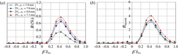
Two examples of actual shapes of spectra (3.1) are illustrated in figures 15 and 16 measured in regimes 1V and 2V, respectively, for the cases of combination modes CF1 and CF2. These spectra are obtained by the spanwise Fourier transform of the distributions like those shown in figure 14(c–f). It is seen that for modes CF1, the receptivity mechanism under study excites only those CF-waves which have positive spanwise wavenumbers (figures 15 a and 16 a), i.e. those propagated upstream the cross-flow and representing the most dangerous CF-instability waves. Almost the same is observed for attenuating modes CF2 (figures 15 b and 16 b), although some weak perturbations are also excited at this combination frequency at low absolute values of negative spanwise wavenumber. Qualitatively similar results are obtained for modes CF1 and CF2 in all other regimes studied.

3.3 Amplification curves and initial wavenumber spectra of excited CF modes

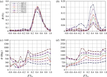
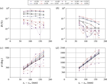
For every fixed value of the spanwise wavenumber, each complex-valued spectrum, such as those shown in figures 15 and 16, gives a streamwise distribution of amplitude $B$ and phase ${\it\phi}$ of the normal CF wave (either CF1 or CF2). An example of such distributions is presented in figure 17 for regime 1V. Similar results were obtained for all other studied regimes. The spectral amplitudes are expressed as a percentage of the local free-stream velocity.

Figure 17.

Streamwise distributions of amplitudes (a,b) and phases (c,d) of normal CF waves measured in regime 1V for modes CF1 (a,c) and CF2 (b,d) with various values of dimensionless spanwise wavenumber ${\it\beta}^{\prime }{\it\delta}_{1v}$ .

The amplification curves for the difference combination waves CF1 of various spanwise wavenumber (as in figure 17 a) display a behaviour that is typical for the CF-instability waves studied in previous experiments (see e.g. Gaponenko et al. Reference Gaponenko, Ivanov and Kachanov1995a ,Reference Gaponenko, Ivanov, Kachanov and Kobayashi b ). At low frequencies $f_{CF1}$ , the modes with the non-dimensional spanwise wavenumbers around 0.4–0.6 (the most amplifying or least attenuating modes in a broad range of frequencies) display a behaviour which is close to neutral on average. They grow slightly at the beginning of the studied streamwise range and start to decay weakly at its end.

The amplification curves obtained for the sum combination modes CF2 (as in figure 17 b) display attenuation in all regimes for all spanwise-wavenumber harmonics, the spectral amplitudes of which are large enough to be measured accurately. (Oscillations observed in figure 17(a–d) correspond usually to very low spectral amplitudes and indicate a poor accuracy of the measurements due to comparable levels of signal and noise.) The attenuation rate increases with frequency, which is consistent with CF-stability theory.

The spectral phases of all studied modes (illustrated in figure 17 c,d) increase downstream in a linear way in all regimes of measurements (1V, 2V, 3V, 4V). The rate of their growth increases with frequency for every fixed value of the spanwise wavenumber. The general behaviour of the normal mode phases is again consistent with previous observations and with CF-stability theory.

The amplification curves (like those presented in figure 17 a,b) were used for estimation of the initial (i.e. at the position of the surface vibrator centre) amplitude spectra of the excited CF waves

as described below. The corresponding phase distributions (like those shown in figure 17 c,d) were used for determination of the initial phase spectra and the initial dispersion curves (2.2).

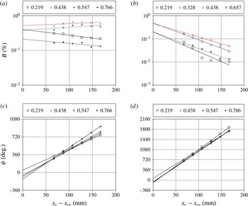
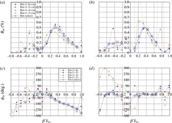
Each initial spanwise-wavenumber spectrum of the excited CF-instability wave was obtained with the help of the streamwise distributions like those shown in figure 17 by means of approximation and upstream extrapolation of the CF-wave spectral amplitudes and phases measured far enough from the surface vibrator (i.e. in the disturbance source far field). The approximations and extrapolations (figure 18) were performed with the help of exponents for the amplitude distributions and straight lines – for the phase distributions. (We did not use in this case the procedure PaL (Parabola-Linear) for the spectral amplitudes (as in several previous works such as Borodulin et al. Reference Borodulin, Ivanov, Kachanov and Roschektayev2013) because the amplitudes of the combinations modes CF1 and CF2 were rather low and, hence, the accuracy of the measurements was also relatively low.) The number of streamwise positions used for approximation was varied, especially when disturbances attenuated quickly downstream, as for modes CF2. Various versions of results, obtained for different numbers of approximated points are illustrated below for comparison (see figure 19).

Figure 18.

Example of extrapolation of experimental data set for regime 1V. Streamwise distributions of normal mode amplitudes (a,b) and phases (c,d) of waves CF1 (a,c) and CF2 (b,d) with various values of dimensionless spanwise wavenumber ${\it\beta}^{\prime }{\it\delta}_{1v}$ .

An example of application of the extrapolation procedures to one experimental data set illustrated in figure 18 corresponds to regime 1V. The streamwise distributions of the normal mode amplitudes and phases are shown in figures 18(a,b) and 18(c,d), respectively, for waves CF1 (figure 18 a,c) and CF2 (figure 18 b,d) and for several values of the spanwise wavenumber ${\it\beta}^{\prime }{\it\delta}_{1v}$ . Lines indicate the results of approximations of the experimental points (for points nos 1–6 in this case). The initial spectral amplitudes and phases were determined in the point $x_{c}-x_{cv}=0$ from the corresponding approximation formulas.

Figure 19.

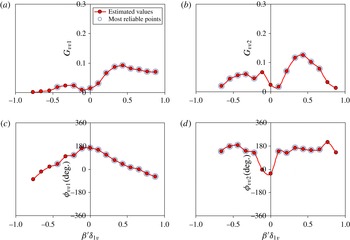
Estimated initial spectral amplitudes (a,b) and phases (c,d) of waves CF1, $f_{CF1}=30$  Hz (a,c) and CF2, $f_{CF2}=110$  Hz (b,d) excited in regime 1V.

The resulting initial amplitude spectra (3.2) of the excited CF waves are illustrated in figure 19(a,b) for the case of regime 1V for waves CF1 and CF2, respectively. The corresponding initial phase spectra are shown in figure 19(c,d). Every plot contains five different initial spectra obtained by means of four different procedures of approximation and extrapolation. Four spectra correspond to approximations, which use streamwise positions: $x_{1}^{\prime }$ – $x_{3}^{\prime }$ , $x_{1}^{\prime }$ – $x_{4}^{\prime }$ , $x_{1}^{\prime }$ – $x_{5}^{\prime }$ and $x_{1}^{\prime }$ – $x_{6}^{\prime }$ and are the same for all spanwise wavenumbers. The fifth spectrum is obtained for the number of points selected individually for every spanwise-wavenumber mode. This fifth spectrum is regarded as the most probable and the most reliable one. The criteria of selection of the number of points used for the extrapolation in the ‘selected’ spectra were the following. The spectral amplitudes in the approximated points have to have downstream behaviour close to the exponential one, while the spectral phases have to increase downstream in a linear way. This kind of behaviour corresponds to the physical sense, as well as to experience of previous investigations, and to behaviour of those spectral modes in the present experiments which have large amplitudes providing low error of measurement.

Figure 19(a,b) illustrates several properties of initial spectral amplitudes valid for all studied regimes (1V, 2V, 3V and 4V). The spectral amplitudes are significantly larger for positive spanwise wavenumbers compared to those with negative ones. This conclusion is valid for the two combination frequencies (excluding mode CF2 in regime 2V). The largest amplitudes are always observed in the range of ${\it\beta}^{\prime }{\it\delta}_{1v}$ between 0.2 and 0.6. The modes with negative spanwise wavenumbers are almost not excited in the flow at the difference combination frequency (waves CF1). For high-frequency combination waves CF2 some initial amplitudes (usually small) are observed even at negative spanwise wavenumbers ${\it\beta}^{\prime }{\it\delta}_{1v}$ between zero and $-0.4$ , especially at the highest frequency $f_{CF2}=124$  Hz and largest value of the parameter of the surface non-stationarity $k=f_{sur}/f_{vor}=2.1$ (regime 2V).

The initial phase spectra (as those shown in figure 19 c,d) have measurable values mainly for positive spanwise wavenumbers. For combination waves CF1 the phases decrease with ${\it\beta}^{\prime }{\it\delta}_{1v}$ in all studied regimes, while for waves CF2 the phase variation with ${\it\beta}^{\prime }{\it\delta}_{1v}$ is much weaker.

Note that the initial phases shown in figure 19(c,d) have been recalculated already by means of time shift ${\rm\Delta}t=-{\it\varphi}_{surrs}/{\it\omega}_{sur}$ (discussed below in the end of § 3.5). This shift is necessary for performing a correct comparison of the phases of the vibration-vortex receptivity coefficients found in the present experiments with those of the roughness-vortex receptivity coefficients found by Borodulin et al. (Reference Borodulin, Ivanov, Kachanov, Roschektayev and Fomin2008a , Reference Borodulin, Ivanov, Kachanov and Roschektayev2013).

The initial spectra like those presented in figure 19 were used for finding the vibration-vortex receptivity coefficients.

3.4 Resonant spectra of surface vibrations

It is found experimentally that the displacement $Y_{m}$ of the vibrator membrane along the $y$ -coordinate from an equilibrium state can be described as $\bar{Y}_{m}({\it\rho},t)=\bar{f}_{m}({\it\rho})\exp (\text{i}{\it\omega}_{sur}t)$ at ${\it\rho}\leqslant R$ , where $R=5$  mm is the radius of the membrane, ${\it\rho}$ is the polar radius with the origin in the centre of the vibrator and $\bar{f}_{m}({\it\rho})=A_{m}({\it\rho})\exp [\text{i}{\it\phi}_{m}({\it\rho})]$ , where $A_{m}({\it\rho})=A_{mo}a_{m}({\it\rho})$ and ${\it\phi}_{m}({\it\rho})={\it\phi}_{mo}+{\it\phi}_{m}({\it\rho})$ are real functions characterizing the amplitude and phase of the membrane oscillations ( $A_{mo}$ and ${\it\phi}_{mo}$ are the amplitude and phase in the membrane centre). The shape function $\bar{f}_{m}({\it\rho})$ is localized in space and can be subjected to double Fourier transform along the $x^{\prime }$ - and $z^{\prime }$ -coordinates using the Fourier integral. Therefore, the complex wavenumber spectrum of the shape of vibrations can be determined as

where $\bar{C}({\it\alpha}_{r}^{\prime },{\it\beta}^{\prime })=C({\it\alpha}_{r}^{\prime },{\it\beta}^{\prime })\exp [\text{i}{\it\lambda}({\it\alpha}_{r}^{\prime },{\it\beta}^{\prime })]$ and C, ${\it\lambda}$ are real spectral amplitude and phase. Then the corresponding non-dimensional (i.e. normalized by $A_{mo}$ ) spectrum of vibrations $\bar{C}^{\prime }({\it\alpha}_{r}^{\prime },{\it\beta}^{\prime })=C^{\prime }({\it\alpha}_{r}^{\prime },{\it\beta}^{\prime })\exp [\text{i}{\it\lambda}({\it\alpha}_{r}^{\prime },{\it\beta}^{\prime })]$ is $\bar{C}^{\prime }({\it\alpha}_{r}^{\prime },{\it\beta}^{\prime })=\bar{C}({\it\alpha}_{r}^{\prime },{\it\beta}^{\prime })/A_{mo}$ . The resonant spectra of vibrations $\tilde{\bar{C}}({\it\alpha}_{r}^{\prime },{\it\beta}^{\prime })=\tilde{C}({\it\alpha}_{r}^{\prime },{\it\beta}^{\prime })\exp [\text{i}\tilde{{\it\lambda}}({\it\alpha}_{r}^{\prime },{\it\beta}^{\prime })]$ for combination modes CF1 and CF2 are defined as $\tilde{\bar{C}}_{1}=\bar{C}({\it\alpha}_{r\,sur1},{\it\beta}_{sur1}^{\prime })$ , and $\tilde{\bar{C}}_{2}=\bar{C}({\it\alpha}_{r\,sur2},{\it\beta}_{sur2}^{\prime })$ , respectively. Shown in figure 20(a) is the membrane shape spectrum (here $K$ is the wavevector length), while the shape of the resonant amplitude spectra (normalized by dimensionless amplitude $A_{mo}/{\it\delta}_{1v}$ ) is illustrated in figure 20(b) for modes CF1 and CF2 measured in regime V2. Note that the membrane shape spectrum is symmetric, while the resonant spectra are not symmetric due to asymmetry of the CF-wave dispersion functions (see figure 13).

Figure 20.

Amplitude and phase parts of wavenumber spectrum of the shape of vibrator oscillations (a) and the resonant amplitude spectra obtained in regime V2 for modes CF1 and CF2 (b).

The measured actual zero-to-peak (not r.m.s.) dimensional amplitudes of the vibrations at the membrane centre $A_{mo}$ found in regimes 1V, 2V, 3V, 4V, $2\text{V}_{1}$ , $2\text{V}_{2}$ and $2\text{V}_{3}$ are: 410, 343, 379, 400, 346, 346 and $346~{\rm\mu}\text{m}$ , respectively.

3.5 Free-stream vortex amplitudes and phases above the surface vibrator

Further components necessary for determination of the receptivity coefficients are the free-stream vortex amplitudes $A_{vorv}$ and phases ${\it\varphi}_{vorv}$ over the surface vibrator. They were determined almost directly from the wall-normal profiles measured at the position of the vibrator centre at the wall-normal location of $y={\it\delta}$ (defined at $U=0.99U_{e}$ ). The amplitudes found in regimes 1V, 2V, 3V, 4V, $2\text{V}_{1}$ , $2\text{V}_{2}$ and $2\text{V}_{3}$ are: 0.77, 0.81, 0.76, 0.72, 0.77, 0.42 and 0.79 %, respectively.

Note that the phases of for all three kinds of perturbations, including the free-stream vortices, used finally for estimation of the receptivity coefficients (3.5), (3.6) (see the next section) were recalculated. They were shifted by values $-{\it\omega}_{CF}{\rm\Delta}t$ , $-{\it\omega}_{vor}{\rm\Delta}t$ and $-{\it\omega}_{sur}{\rm\Delta}t$ for CF-, vortical, and vibrational disturbance, respectively. Here ${\rm\Delta}t=-{\it\varphi}_{surrs}/{\it\omega}_{sur}$ and ${\it\varphi}_{surrs}$ is the phase of vibrations measured relative to the reference signal. After this recalculation, all disturbance phases were counted not relative to an arbitrary time instant $t_{1}$ of the reference signal but relative to the time-axis origin, which coincides with the time instant $t_{o}=t_{1}-{\rm\Delta}t$ corresponding to maximum positive (convex) deflection of the surface vibrator membrane. After this recalculation, the initial phase of the vibrations becomes equal to zero. As was indicated by Würz et al. (Reference Würz, Herr, Wörner, Rist, Wagner and Kachanov2003), phases of this kind are convenient for extrapolation of the receptivity characteristics to the zero frequency of vibrations and for comparison of these characteristics with those obtained at scattering of the free-stream disturbances on steady surface non-uniformities. In the present case, this point is important for comparison of the obtained receptivity phases with those obtained in experiments by Borodulin et al. (Reference Borodulin, Ivanov, Kachanov, Roschektayev and Fomin2008b , Reference Borodulin, Ivanov, Kachanov and Roschektayev2013). For the regimes indicated above (1V, 2V, 3V, 4V, $2\text{V}_{1}$ , $2\text{V}_{2}$ and $2\text{V}_{3}$ ) the recalculated phases of free-stream vortices are found to have the following values: 216, 242, 159, 221, 245, 242 and 246.

3.6 Definition of receptivity coefficients

In every regime of measurement (with excitation of combination CF-modes CF1 and CF2 having definite fixed frequencies) we define the complex vibration-vortex receptivity-coefficient (function)

(where $G_{vv\,1,2}$ and ${\it\phi}_{vv\,1,2}$ are the corresponding real receptivity amplitudes and phases) as follows

where $\tilde{\bar{C}}_{1,2}=\bar{C}({\it\alpha}_{r\,sur1,2},{\it\beta}_{sur1,2}^{\prime })$ are the corresponding resonant spectra of vibrations discussed above and $\bar{B}_{in\,1,2}({\it\beta}_{CF\,1,2}^{\prime })=\bar{B}_{in}({\it\omega}_{CF\,1,2},{\it\beta}_{CF\,1,2}^{\prime })$ are the corresponding initial spectra of modes CF1 and CF2. Separately for amplitudes and phases, the definition (3.5) means:

It is important to note in the end of this section that the definition of the complex-valued receptivity coefficient $\bar{G}_{vv}$ for the vibration-vortex receptivity is somewhat different from that given by Borodulin et al. (Reference Borodulin, Ivanov, Kachanov, Roschektayev and Fomin2008b , Reference Borodulin, Ivanov, Kachanov and Roschektayev2013) for the roughness-vortex receptivity problem ( $\bar{G}_{rv}$ ). At the same time, these coefficients are comparable with each other directly. This point is explained in the following way. In the definition of coefficient $\bar{G}_{vv}$ the initial spectrum of CF waves corresponds to Fourier integral (3.1), while for coefficient $\bar{G}_{rv}$ it corresponds to Fourier series. The normalization is different. However, the same difference is present in the definitions of the corresponding resonant spanwise-wavenumber spectra of the surface non-uniformities. Therefore, the ratios present in formulas such as (3.5) and (3.6) are independent from the way of normalization, providing the same dimensionality and comparability of the receptivity coefficients in these two experiments.

6.1 Vibration-vortex receptivity coefficients

The receptivity coefficients described in this and the next subsections represent the most important result of the present experiments.

The estimated dimensionless vibration-vortex receptivity-coefficient amplitudes are illustrated in figures 28(a,b), 29(a,b), 30(a,b) and 31(a,b) for regimes 1V, 2V, 3V and 4V, respectively, versus the dimensionless spanwise wavenumber of the excited CF wave. Plots (a) correspond to difference combination modes CF1, while plots (b) are obtained for sum combination modes CF2. The corresponding phases of the receptivity coefficients are shown in figures 28(c,d), 29(c,d), 30(c,d) and 31(c,d) for regimes 1V, 2V, 3V and 4V, respectively. The most reliable data (i.e. those having reasonably nice approximation and extrapolation of the amplification curves) are shown in figures 28–31 with large open circles; the accuracy of the other points is poor. The receptivity amplitudes are obtained with the following normalizations. All velocity-fluctuation amplitudes are presented as a percentage of the free-stream velocity over the centre of the vibrator $U_{ev}=6.5~\text{m s}^{-1}$ . All spatial variables (including the amplitudes of vibration) are divided by the boundary-layer displacement thickness at the vibrator position ${\it\delta}_{1v}=1.23$  mm. The phases are counted from the time instant $t_{o}$ , which corresponds to the maximum positive deflection of the vibrator membrane. Such a definition is convenient for comparison of the receptivity phases obtained in different regimes with each other and with those found in experiments by Borodulin et al. (Reference Borodulin, Ivanov, Kachanov, Roschektayev and Fomin2008b , Reference Borodulin, Ivanov, Kachanov and Roschektayev2013) for scattering of vortices on steady surface non-uniformity.

Figure 28.

Dimensionless receptivity-coefficient amplitudes (a,b) and phases (c,d) obtained in regime 1V for modes CF1, $f_{CF1}=30$  Hz (a,c) and CF2, $f_{CF2}=110$  Hz (b,d) versus dimensionless CF-wave spanwise wavenumber.

The vibration-vortex receptivity amplitudes turned out to be much greater for CF-modes with positive spanwise wavenumbers compared to those with negative ones. This general feature is common for waves CF1 and CF2 (excluding one case of mode CF2 in regime 2V shown in figure 29 b). The largest receptivity amplitudes are observed in a range of spanwise wavenumbers ${\it\beta}^{\prime }{\it\delta}_{1v}$ between $+0.2$ and $+0.8$ approximately. (Note that this range includes the most amplifying (or least attenuating) cross-flow instability modes.) Some non-zero receptivity amplitudes are also observed at negative values of ${\it\beta}^{\prime }{\it\delta}_{1v}$ (around $-0.25$ ), especially for wave CF2 (figures 28 b, 29 b, 30 b and 31 b) and especially in regime 2V (figure 29 b) with the highest frequencies $f_{sur}=84$  Hz, $f_{CF1}=44$  Hz, $f_{CF2}=124$  Hz and largest value of parameter of the surface vibration non-stationarity $k=2.1$ . Note, however, that such high-frequency modes are much less important for the present swept-wing transition problem because of their attenuation or weaker amplification.

Figure 29.

Dimensionless receptivity-coefficient amplitudes (a,b) and phases (c,d) obtained in regime 2V for modes CF1, $f_{CF1}=44$  Hz (a,c) and CF2, $f_{CF2}=124$  Hz (b,d) versus dimensionless CF-wave spanwise wavenumber.

Figure 30.

Dimensionless receptivity-coefficient amplitudes (a,b) and phases (c,d) obtained in regime 3V for modes CF1, $f_{CF1}=16$  Hz (a,c) and CF2, $f_{CF2}=96$  Hz (b,d) versus dimensionless CF-wave spanwise wavenumber.

Figure 31.

Dimensionless receptivity-coefficient amplitudes (a,b) and phases (c,d) obtained in regime 4V for modes CF1, $f_{CF1}=16$  Hz (a,c) and CF2, $f_{CF2}=124$  Hz (b,d) versus dimensionless CF-wave spanwise wavenumber.

Meanwhile, the receptivity amplitudes, obtained at ${\it\beta}^{\prime }<0$ for low frequencies corresponding to the frequency range of the CF instability (as waves CF1 with $f_{CF1}=16$  Hz in regimes 3V and 4V presented in figures 30 a, 31 a) are immeasurably small. A very significant dependence of the receptivity amplitudes on type of the combination CF-mode (CF1 or CF2) and on regime of measurement is found. This dependence will be analysed below.

The receptivity phases display a significantly more conservative behaviour compared to the receptivity amplitudes, especially within every particular kind of combination wave. This property is consistent with previous observations (Gaponenko et al. Reference Gaponenko, Ivanov, Kachanov and Crouch2002) for the swept-wing boundary-layer receptivity to surface non-uniformities. For mode CF1 the receptivity phases decrease with the spanwise wavenumber rather quickly (figures 28 c, 29 c, 30 c and 31 c) in an almost linear way in all studied regimes, while for mode CF2 this dependence is either significantly weaker (as in regimes 3V and 4V, figures 30 d, 31 d) or is practically absent (as in regimes 1V and 2V, figures 28 d, 29 d), at least in the spanwise-wavenumber ranges of the most reliable data.

6.2 Comparison of vibration- and roughness-vortex receptivity coefficients

We now concentrate on the dependence of the receptivity coefficients on other disturbance parameters and, simultaneously, on comparison of the vibration-vortex receptivity coefficients $\bar{G}_{vv}$ with the roughness-vortex receptivity coefficients $\bar{G}_{rv}$ obtained by Borodulin et al. (Reference Borodulin, Ivanov, Kachanov, Roschektayev and Fomin2008b , Reference Borodulin, Ivanov, Kachanov and Roschektayev2013) for zero frequency of surface non-uniformities. The dependence of the receptivity amplitudes on the frequency of surface vibrations $f_{sur}$ is presented in figure 32 for a fixed value of the free-stream vortex frequency $f_{vor}=40$  Hz. The results are presented in a range of values of the spanwise wavenumber covering the value ( ${\it\beta}^{\prime }{\it\delta}_{1v}=0.617$ ) studied in experiments by Borodulin et al. (Reference Borodulin, Ivanov, Kachanov, Roschektayev and Fomin2008b , Reference Borodulin, Ivanov, Kachanov and Roschektayev2013). Lines in figure 32 correspond to the exponential curve fit for the present data. It is seen, first, that the vibration-vortex receptivity coefficients estimated in the present experiments have an exponential dependence on $f_{sur}$ and, second, the exponents hit almost exactly the value of the receptivity amplitude 0.0054 found in experiments by Borodulin et al. (Reference Borodulin, Ivanov, Kachanov, Roschektayev and Fomin2008b , Reference Borodulin, Ivanov, Kachanov and Roschektayev2013) for the zero frequency of the surface non-uniformity!

Figure 32.

Dependence of the vibration- and roughness-vortex receptivity coefficients on surface vibration frequency measured at $f_{vor}=40$  Hz in regimes 1V, 2V and 3V for mode CF1 and in regime 1R ( $f_{sur}=0$ ) by Borodulin et al. (Reference Borodulin, Ivanov, Kachanov, Roschektayev and Fomin2008b , Reference Borodulin, Ivanov, Kachanov and Roschektayev2013). Lines – exponential approximations.

However, the receptivity-amplitude dependence on frequency $f_{CF}$ of the excited CF-waves illustrated in figure 33 displays a significant difference between the behaviour of the receptivity-coefficient amplitudes $G_{vv}$ and $G_{rv}$ . The results presented in this figure are obtained for a fixed absolute value of the non-dimensional spanwise wavenumbers $|{\it\beta}^{\prime }{\it\delta}_{1r}|=|{\it\beta}^{\prime }{\it\delta}_{1v}|=0.618$ . In the present experiments, values of ${\it\beta}^{\prime }$ are always positive, while in experiments by Borodulin et al. (Reference Borodulin, Ivanov, Kachanov, Roschektayev and Fomin2008b , Reference Borodulin, Ivanov, Kachanov and Roschektayev2013) they are both positive and negative. It is seen that both the vibration-vortex receptivity amplitudes (obtained in the present experiments for mode CF1) and the roughness-vortex receptivity amplitudes (obtained by Borodulin et al. (Reference Borodulin, Ivanov, Kachanov, Roschektayev and Fomin2008b , Reference Borodulin, Ivanov, Kachanov and Roschektayev2013) for the two combination modes) grow with $f_{CF}$ in a linear way, but the rates of their growth are very much different. Moreover, the vibration-vortex receptivity amplitudes obtained for mode CF2 display a very strong deviation from all other points.

Figure 33.

Dependence of the vibration- and roughness-vortex receptivity coefficients on CF-wave frequency measured at various $f_{vor}$ in regimes 1V, 2V, 3V, 4V for modes CF1 and CF2 and in regimes 1R, 2R, 3R ( $f_{sur}=0$ ) by Borodulin et al. (Reference Borodulin, Ivanov, Kachanov, Roschektayev and Fomin2008b , Reference Borodulin, Ivanov, Kachanov and Roschektayev2013). Lines – linear approximations. ${\it\beta}^{\prime }{\it\delta}_{1v}=0.618$ , $|{\it\beta}^{\prime }{\it\delta}_{1r}|=0.618$ .

Figure 34.

Dependence of the vibration- and roughness-vortex receptivity coefficients on the parameter of surface non-stationarity $k$ obtained in regimes 1V, 2V, 3V, 4V for modes CF1 and CF2 (various $f_{vor}$ and $f_{sur}$ ) and in regimes 1R, 2R, 3R in experiments by Borodulin et al. (Reference Borodulin, Ivanov, Kachanov, Roschektayev and Fomin2008b , Reference Borodulin, Ivanov, Kachanov and Roschektayev2013) (various $f_{vor}$ but $f_{sur}=0$ ) for $|{\it\beta}^{\prime }{\it\delta}_{1r}|={\it\beta}^{\prime }{\it\delta}_{1v}=0.618$ .

These distinctions are clearly associated with very strong difference in the frequencies of the surface non-uniformities in these two experiments, i.e. with a degree of the surface-shape non-stationarity. Following experiments by Ivanov et al. (Reference Ivanov, Würz, Herr, Wagner and Kachanov2005), this degree can be characterized by the parameter of the surface non-stationarity $k=f_{sur}/f_{vor}$ . Indeed, utilizing of this parameter as an argument presented in figure 34 leads to striking changes. In contrast to figure 33, a good correlation of all receptivity amplitudes obtained in various regimes (for both $G_{vv}$ and $G_{rv}$ coefficients and for modes CF1 and CF2) is now observed! The line in this figure corresponds to the exponential approximation of all the experimental points obtained in all the regimes mentioned above. This result shows also that the boundary-layer receptivity increases significantly with the parameter $k$ and remains very low for both stationary and low-frequency surface non-uniformities. This circumstance explains why the authors of the experiments by Borodulin et al. (Reference Borodulin, Ivanov, Kachanov, Roschektayev and Fomin2008b , Reference Borodulin, Ivanov, Kachanov and Roschektayev2013) were forced to use a special technique of ‘phased roughness’ to be able to obtain such low values of the receptivity amplitudes.

Based on experience of previous measurements and on physical considerations, one can assume that there is one more parameter important for the vortex receptivity mechanisms, which could be useful for the analysis and interpretation of the experimental data obtained in different regimes. This parameter corresponds to the angle of orientation of the excited CF-wave front with respect to the free-stream vortex axis. One can expect that the receptivity has to increase when this angle gets smaller and it has to go to zero (at least in two-dimensional flows) when this angle tends to 90°. In the present experiments this angle was defined as ${\rm\Delta}{\it\theta}_{axis}=\min \{|({\it\theta}_{CF}-{\it\theta}_{vor})|,|({\it\theta}_{CF}-{\it\theta}_{vor})+180^{\circ }|,|({\it\theta}_{CF}-{\it\theta}_{vor})+180^{\circ }|\}$ . The corresponding angular distributions of the receptivity amplitudes $G_{vv}$ and $G_{rv}$ are presented in figure 35 for all studied modes with ${\it\beta}^{\prime }{\it\delta}_{1v}=|{\it\beta}^{\prime }{\it\delta}_{1r}|=0.618$ . It is seen that the receptivity amplitudes decrease with ${\rm\Delta}{\it\theta}_{axis}$ for mode CF1 (with ${\it\beta}^{\prime }{\it\delta}_{1v}=+0.618$ ) in the present experiments and for the two combination modes (with ${\it\beta}^{\prime }{\it\delta}_{1r}=+0.618$ and $-0.618$ ) in experiments by Borodulin et al. (Reference Borodulin, Ivanov, Kachanov, Roschektayev and Fomin2008b , Reference Borodulin, Ivanov, Kachanov and Roschektayev2013). (For mode CF2 in the present experiments the correlation is absent.) The general tendencies for the receptivity-coefficient amplitudes $G_{vv}$ and $G_{rv}$ are the same despite the fact that their values are different. This very important fact indicates that the receptivity to free-stream vortices has to be much larger in the case when the vortex axes are directed along the cross-flow vortex (wave) axes compared to the presently studied cases of relatively large angles (above 60°).

Figure 35.

Dependence of the vibration- and roughness-vortex receptivity coefficients on angle ${\rm\Delta}{\it\theta}_{axis}$ between the free-stream vortex axis and the CF-wave front obtained in regimes 1V, 2V, 3V, 4V for modes CF1 and CF2 (various $f_{vor}$ and $f_{sur}$ ) and in regimes 1R, 2R, 3R in experiments by Borodulin et al. (Reference Borodulin, Ivanov, Kachanov, Roschektayev and Fomin2008b , Reference Borodulin, Ivanov, Kachanov and Roschektayev2013) (various $f_{vor}$ but $f_{sur}=0$ ) for $|{\it\beta}^{\prime }{\it\delta}_{1r}|={\it\beta}^{\prime }{\it\delta}_{1v}=0.618$ .