1. Introduction
Maritime transport is a cornerstone of the global economy, carrying over 80% of the volume of international trade in goods, with this percentage being even higher in many developing countries (UNCTAD, 2021). Maritime transport supports the efficient operation of international logistics supply chains, thereby promoting global economic and trade development. However, as the volume of seaborne trade continues to grow, the environmental impact of maritime transport, particularly in terms of carbon dioxide (CO2) emissions, has become a significant concern. The International Maritime Organization (IMO) reports that global greenhouse gas (GHG) emissions from shipping have reached 1.076 billion tons, making the shipping industry the fifth-largest emitter of CO2 worldwide (IMO, 2021; BP Group, 2021). If current trends persist, these emissions could increase by 50% to as much as 250% by 2050, highlighting the urgent need for effective mitigation strategies.
In response to this growing environmental challenge, the IMO adopted a long-term emissions reduction strategy in 2018, setting a target to reduce maritime GHG emissions by 50% by 2050, regardless of the anticipated growth in maritime trade (Di Natale and Carotenuto, Reference Di Natale and Carotenuto2015). Despite the ambitious nature of this target, there are concerns that it may not be sufficient to meet the Paris Agreement’s goal of limiting global warming to 1.5°C (Bullock et al., Reference Bullock, Mason and Larkin2022). Consequently, the International Chamber of Shipping (ICS) has called on the IMO to urge governments to take more immediate and substantial actions to help the global maritime sector achieve net-zero carbon emissions by 2050 (Başhan and Kökkülünk, Reference Başhan and Kökkülünk2020; McKinlay et al., Reference McKinlay, Turnock and Hudson2021).
Current methodologies for estimating ship CO2 emissions are primarily divided into two approaches, referred to here as top-down and bottom-up approaches. Top-down methods rely on macro-statistical data and are mainly categorised as either fuel-based or trade-based approaches. The fuel-based method estimates total emissions by multiplying the ship’s fuel consumption by the relevant emission factors (Endresen et al., Reference Endresen, Sørgård, Behrens, Brett and Isaksen2007; Tzannatos, Reference Tzannatos2010). This approach benefits from straightforward data collection and can quickly estimate emissions across large sea areas. However, it lacks specificity regarding individual ship characteristics, resulting in high uncertainty in its estimates. The trade-based method estimates emissions by evaluating ship fuel consumption through cargo turnover and type data and then applying emission factors (Streets et al., Reference Streets, Guttikunda and Carmichael2000; Yang et al., Reference Yang, Ma and Xing2017). While this method can correlate ship emissions with economic indicators, its reliance on numerous assumptions reduces the confidence in the results. Generally, top-down methods, with their broader data granularity, are suitable for estimating CO2 emissions over wide sea areas and analysing long-term trends, but they often fall short in terms of accuracy and certainty (Peng et al., Reference Peng, Wen, Wu, Xiao, Zhou and Han2020).
Advancements in ship equipment and big data technology have led to the increasing prevalence of bottom-up methods in recent years. These methods estimate CO2 emissions based on detailed ship activity trajectories, providing a more precise and reliable assessments of emissions (Peng et al., Reference Peng, Wen, Wu, Xiao, Zhou and Han2020). By using specific operational data from individual ships, bottom-up approaches can significantly enhance the accuracy of emission inventories, supporting more informed policy and regulatory decisions aimed at mitigating the environmental impact of maritime transport.
The introduction of the Automatic Identification System (AIS) has markedly improved the availability of ship data, thereby facilitating the increased use of bottom-up methodologies in emission studies (Alver et al., Reference Alver, Saraç and Şahin2018; Chen et al., Reference Chen, Zhao, Nelson, Li, Wang, Zhou, Lang and Guo2016). The use of AIS data has become a mainstream method for creating these inventories, offering enhanced precision in capturing the real-time operating conditions of ships (Li et al., Reference Li, Yuan, Ou, Fan, Ye, Xiao, Shi, Huang, Ng and Zhong2016; Ng et al., Reference Ng, Loh, Lin, Booth, Chan, Yip, Li and Lau2013). Studies conducted in major port areas, such as the Yangtze River Delta and the Pearl River Delta, have demonstrated the effectiveness of AIS data in assessing and managing ship emissions (Song, Reference Song2015; Xing et al., Reference Xing, Duan, Huang and Liu2016).
This study leverages data from multiple vessel-position transmitting systems, specifically AIS, V-Pass and LTE-Maritime (LTE-M), to estimate maritime carbon dioxide emissions in the coastal waters of South Korea. The primary objective is to develop a comprehensive and spatially explicit assessment framework that addresses the limitations of conventional single-source approaches. The principal contributions of this research are threefold. First, the study integrates trajectory data from three complementary systems: AIS for general maritime traffic, V-Pass for small-scale fishing vessels and LTE-M for high-frequency position reporting. By combining these heterogeneous data sources, the framework overcomes the incomplete vessel coverage inherent in AIS-only inventories, particularly for fishing vessels and small coastal craft that constitute a significant yet often underrepresented segment of maritime activities. Second, the research employs a bottom-up emission estimation approach coupled with a grid-based spatial allocation algorithm at 0.01° resolution (approximately 1 km2). This methodology enables spatially explicit mapping of CO2 emissions, facilitating the identification of emission hotspots and providing greater reliability than conventional top-down methods that rely on aggregated fuel consumption statistics.
Third, the study provides granular emission profiles disaggregated by major port facilities and vessel categories, including cargo ships, tankers, fishing vessels, passenger ships and towing vessels. These detailed emission inventories offer empirical foundations for targeted mitigation strategies and evidence-based policy formulation in maritime environmental management, enabling decision-makers to prioritise interventions based on port-specific operational characteristics and dominant emission sources.
The remainder of the paper is organised as follows. The methodology of this study, including its allocation in grid cells, is presented in Section 2. The carbon dioxide emission measurement results are analysed and discussed in Section 3. Finally, conclusions are given in Section 4.
2. Methodology
2.1. Study area and data collection
This study focuses on the coastal regions of South Korea, encompassing its major ports. Data for this study were sourced from various authoritative maritime agencies. Specifically, AIS and LTE-M data were obtained from the Ministry of Oceans and Fisheries, while V-Pass data were collected from the Korea Coast Guard. The data collected for this study span a 20-day period from May 1, 2021, to May 20, 2021. This timeframe was chosen to ensure consistency and comparability across all datasets. V-pass data, which represents a position-reporting system for fishing vessels in Korea, have proven to be highly effective for both monitoring and researching fishing vessel activities. V-pass is one of the time-series marine traffic monitoring systems developed and distributed by the Republic of Korea in 2015 (Park et al., Reference Park, Jung and Choi2023). According to Korean law, fishing vessels under ten tonnes must be equipped with this reporting system, while those over ten tonnes are required to install the Automatic Identification System (AIS). The V-pass terminal, which is installed on fishing vessels, serves as a critical component for establishing a rapid response system for marine accidents and emergencies. This terminal’s primary function is to transmit the positions of fishing vessels to facilitate quick responses to incidents and emergency situations. When the SOS button on the terminal is activated or if the transmission/reception antenna is detached, an automatic SOS alert is sent to the Korea Coast Guard Rescue Coordination Center (RCC). Additionally, the system is integrated with an automatic departure and entry system, allowing vessel operators to report departures and arrivals without physically visiting a police station or branch office. The location data transmitted from the fishing vessels to land relay stations can experience delays ranging from thirty seconds to seven minutes, depending on transmission conditions. Most V-pass terminals are configured to transmit their current location to land receivers approximately every thirty seconds. The widespread implementation of this system across all fishing vessels has facilitated the precise monitoring and investigation of the exact positions and navigation patterns of fishing vessels operating in Korean coastal waters (Jung et al., Reference Jung, Park and Choi2023).
In 2021, Korea deployed the high-speed maritime wireless communication system, LTE-Maritime, in response to the IMO’s proposal to introduce an e-Navigation system (Jo et al., Reference Jo, Jang, Yu and Shim2018). The LTE-M network, capable of transmitting large volumes of data at an average communication speed exceeding 10 Mbps, offers speeds up to 1,000 times faster than those of the AIS. The establishment of the LTE-M infrastructure, based on a vessel router system, has overcome the limitations of terrestrial LTE communication, providing a communication range of up to 100 km at sea and enabling the transmission of high-density, large-scale information (Jeong et al., Reference Jeong, Natsagdor and Jung2018). Consequently, e-Navigation services using LTE-M were launched in 2021, providing a technological foundation for monitoring vessel positions at a much higher frequency compared with the existing AIS. The maritime wireless communication service employing LTE-M has significantly enhanced the speed and capacity with regards to the transmittance and reception of large volumes of data, with a communication range extending up to 100 km. Theoretically, while AIS is designed to transmit and receive data at intervals ranging from a minimum of two seconds to a maximum of three minutes, LTE-M is engineered to facilitate data transmission and reception at one-second intervals. This advancement in maritime communication technology represents a substantial improvement in the real-time monitoring and management of vessel activities, offering unprecedented capabilities for maritime safety, security and efficiency (Min et al., Reference Min, Lee, Cho, Baek and Park2022).
2.2. Bottom-up methodology
Figure 1 presents the architecture of a carbon emission monitoring system based on vessel-position information. Initially, data from AIS, V-Pass and LTE-M are collected to obtain the vessel-position information. Subsequently, the data are sorted by vessel ID and by the timestamp of data reception. In the preprocessing stage of this study, static information associated with each vessel ID, specifically the vessel type and length, was extracted. The gross tonnage of each vessel was then estimated based on this static information. Following the estimation of the gross tonnage, the main engine power was calculated using the derived tonnage. This estimation of the main engine power subsequently served as the basis for estimating the generator power. This systematic preprocessing approach ensured the accuracy and reliability of the data, providing a robust foundation for subsequent analyses and calculations.
Vessel-position information-based carbon emission monitoring system architecture.

Finally, the CO2 emissions for each vessel type are calculated within each grid cell. In the visualisation stage of the computed results, all files containing the CO2 emissions data for each grid are retrieved. These files, organised on a daily basis, are then aggregated to calculate the cumulative emissions for each grid cell. Subsequently, the aggregated data are visualised using various formats, specifically grid-based maps, bar graphs and pie charts. This approach enables a comprehensive and multifaceted representation of the CO2 emissions data, facilitating a clearer understanding of the spatial and temporal distribution of maritime carbon emissions.
By employing these different visualisation techniques, the study ensures that the complex data on CO2 emissions is accessible and interpretable, allowing for more effective analysis and decision-making. The use of grid-based visualisation helps to pinpoint specific areas with higher emissions, while bar graphs and pie charts offer a straightforward comparison of emissions across different regions or time periods. This methodical approach to data visualisation underscores the importance of accurately representing data to inform policy and regulatory decisions aimed at mitigating the impact of maritime activities on global climate change. The calculation of carbon emissions within a specific grid cell, based on vessel trajectory data, can be represented by the following equation:
 ${E_{i,j,k,n}} = \mathop \sum \limits_{n = 1}^N {P_{j,n}} \times L{F_{j,k,n}} \times E{F_{i,j,n}}\times {T_{j,k,n}}$
Here,
 ${E_{i,j,k,n}}$
represents the carbon dioxide emission for corresponding ship type i under power equipment type j in operating condition k for the n-th ship in a grid, the unit is g; P represents the power of the installed equipment in the engine room, the unit is kW;
 $LF$
represents the ship load factor; EF represents the emission factor, the unit is g/kWh; and
 $T$
represents the operating time.
The types of power equipment on ships include the main engines, generators and boilers. The main engine operates during cruising and manoeuvring to provide propulsion power. The generator operates in all operating modes to produce electricity for lighting, cooking, air conditioning, heating, pumps, auxiliary blowers and the bow thruster. The boiler operates for fuel heating, cargo heating, steam-driven cargo pumps and for the hot water supply (USEPA, 2009).
2.3. Model parameters
Based on Equation (1), the main parameters of the ship exhaust emission estimation model are the ship speed, activity time, the power of the ship equipment, the load factor and the emission factor. These parameters must be collected and processed beforehand to ensure accurate emission calculations. Given that ship exhaust emissions vary under different operating conditions, it is necessary to identify the operating conditions and calculate the emissions separately for each condition. The operating conditions are divided into three stages: cruising, manoeuvring and hotelling. Cruising refers to the period when the pilot boards the ship outside the port area and the vessel navigates within the port boundaries at the speed limit. Emissions during this stage must be calculated by considering the time spent as well as the load factors of the main engine and generators. Manoeuvring involves adjusting the vessel’s speed and position, during which time, the captain or pilot frequently uses the main engine, auxiliary engines, thrusters and rudder to dock the ship safely. The ship’s forward, backward and lateral movements are active due to the constant use of the main engine to reduce the speed and ensure safe docking. Hotelling occurs after the vessel has safely docked and the main engine is turned off. During this stage, generators run to supply power for cargo handling operations, heating and cooling. Emissions are calculated by considering the hotelling time and the load factor of the generators, which is assumed to be 40%, identical to that of the boilers (Lauretis et al., Reference Lauretis, Ntziachristos and Trozzi2023). Hotelling is characterised by speeds of less than 1 knot, manoeuvring as speeds between 1 and 5 knots, and cruising as speeds above 5 knots, reflecting previous studies (Ng et al., Reference Ng, Loh, Lin, Booth, Chan, Yip, Li and Lau2013; Chen et al., Reference Chen, Wang, Nelson, Li, Zhao, Zhao, Lang, Zhou and Guo2017; Li et al., Reference Li, Jia, Wang, Yang, Wang and Kuang2023).
To calculate emissions from different types of ships, vessels in the research area are categorised into six types: cargo ships, passenger ships, tankers, tugs, fishing vessels and other vessels (Ye et al., Reference Ye, Zheng, Pan, Wang and Zhong2014). The installed engine power of a ship is a crucial parameter when estimating its emissions. The relationship between the ship length and gross tonnage is used to estimate the engine power (Gan et al., Reference Gan, Che, Zhou, Zhou, Zheng, Zhang and Song2022). Subsequently, the power output of the generators is estimated as the ratio of the main engine power, following research by the USEPA (2009).
The ship load factor, which is the percentage of the actual output power relative to the installed capacity of the ship’s power equipment, determines the fuel combustion efficiency (Jalkanen et al., Reference Jalkanen, Brink, Kalli, Pettersson, Kukkonen and Stipa2009). The load factor for the ship’s main engine was sourced from Lauretis et al. (Reference Lauretis, Ntziachristos and Trozzi2023).
2.4. Allocation in a grid cell
The ship activity allocation method, as described by Goldsworthy and Goldsworthy (Reference Goldsworthy and Goldsworthy2015), assigns emissions to a grid cell based on the proportion of the vessel’s trajectory length that falls within that cell. In Equation (1), the operating time is allocated to each grid cell based on the distance ratio derived from two sets of vessel trajectory data. This method ensures the precise allocation of the navigation time across different grid cells, accurately reflecting the vessel’s movement and providing a robust foundation for subsequent emission calculations. For instance, as illustrated in Figure 2, the distance and navigation time between the first set of vessel trajectory data and the second set are initially calculated. In this context, the haversine formula, which calculates the great-circle distance between two points on a sphere, is applied to determine the distance travelled between the two points, as shown in Equation (2). The haversine formula is particularly suitable for maritime applications due to its ability to account for the curvature of the earth, thus offering more accurate distance measurements, which are essential for reliable data analysis in marine studies (Sofwan et al., Reference Sofwan, Soetrisno, Ramadhani, Rahmayani, Handoyo and Arfan2019).
 $d = 2r \,\arcsin\!\left(\sqrt{\sin^2\!\left(\frac{\mathrm{lat}_{t+1} - \mathrm{lat}_t}{2}\right) + \cos(\mathrm{lat}_t)\cos(\mathrm{lat}_{t+1}) \sin^2\!\left(\frac{\mathrm{lon}_{t+1} - \mathrm{lon}_t}{2}\right)}\right)$
Grid representation of a ship trajectory segment.

In Equation (2),
 ${{la}}{{{t}}_t}$
and
 $\;{{lon}_t}$
are the latitude and longitude at time t, respectively, and
 ${{la}}{{{t}}_{t + 1}}$
and
 ${{lon}_{t + 1}}$
are correspondingly the latitude and longitude at time t+1.
 $r$
represents the radius of the earth.
To extract the grid cells traversed between the first and second trajectory data points, it is necessary to identify their intersection points, which are derived using equations for two lines. The equation of the first line, which represents the trajectory, has the form y = ax + b. This equation is calculated from the coordinates (longitude and latitude) of the two trajectory data points
 ${p_t}$
and
 ${p_{t + 1}}$
. The equation of the second line represents the grid boundaries, either y = c for the x-axis or x = c for the y-axis. This approach ensures precise identification of the grid cells through which the vessel passes.
As illustrated in Figure 2(c), nine grid cells were identified. To extract these grid cells accurately, it is necessary to determine the direction of the vessel’s movement, such as whether it is moving southward, eastward or in any other direction. By assessing the direction of movement, the corresponding grid cell numbers can be identified. This direction-based identification method ensures the precise mapping of the vessel’s trajectory within the grid system.
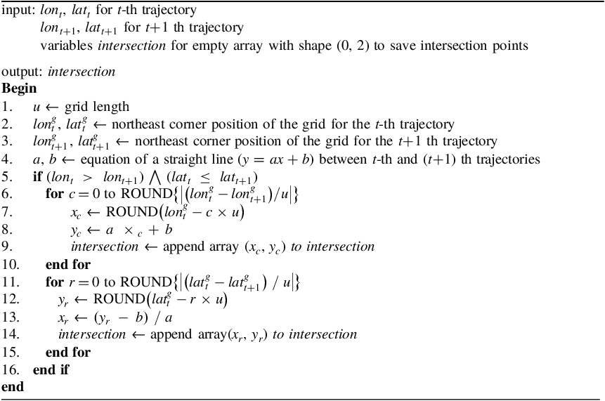
The direction search is conducted by comparing the latitudes and longitudes of the t-th trajectory data with the (t+1)-th trajectory data based on the following four conditions:
 \[
\begin{cases}
\text{W or NW: } (lon_t > lon_{t+1}) \wedge (lat_t \le lat_{t+1}) \\
\text{N or NE: } (lon_t \le lon_{t+1}) \wedge (lat_t < lat_{t+1}) \\
\text{E or SE: } (lon_t < lon_{t+1}) \wedge (lat_t \ge lat_{t+1}) \\
\text{S or SW: } (lon_t \ge lon_{t+1}) \wedge (lat_t > lat_{t+1})
\end{cases}
\]
The pseudocode in Algorithm 1 demonstrates the process for identifying intersection points when the vessel trajectory data indicate a direction of W or NW. The intersections are categorised into two types: intersections with lines parallel to the y-axis and intersections with lines parallel to the x-axis. First, the extraction of intersection points with lines parallel to the y-axis proceeds as follows. Calculate the integer value obtained by dividing the difference between the longitudes of the grid containing the t-th trajectory data (
 ${\rm{lon}}_t^g$
) and the (t+1)-th trajectory data (
 ${\rm{lon}}_{t + 1}^g$
) by the grid interval u. Subtract the product of the grid interval u and c from the longitude of the grid containing the t-th trajectory data (
 ${\rm{lon}}_t^g$
) to determine the longitude
 ${x_c}$
of the c-th intersection. Then, using the equation of the line, calculate the latitude
 ${y_c}$
corresponding to
 ${x_c}$
. This method allows for the extraction of intersection points with lines parallel to the y-axis.
Next, the extraction of intersection points with lines parallel to the x-axis proceeds as follows. Calculate the integer value obtained by dividing the difference between the latitudes of the grid containing the t-th trajectory data (
 ${\rm{lat}}_t^g$
) and the (t+1)-th trajectory data (
 ${\rm{lat}}_{t + 1}^g$
) by the grid interval u. Subtract the product of the grid interval μ and r from the latitude of the grid containing the t-th trajectory data (
 ${\rm{lat}}_t^g$
) to determine the latitude
 ${y_r}$
of the r-th intersection. Then, using the equation of the line, calculate the longitude
 ${x_r}$
corresponding to
 ${y_r}$
. This method allows for the extraction of intersection points with lines parallel to the x-axis. By following these detailed steps, the precise intersection points for each grid can be identified, enabling the accurate mapping of the vessel’s trajectory within the grid system.
Extraction of intersection points by direction – W or NW

3. Results and discussion
3.1. Results
To monitor carbon emissions along the coast, it is essential to calculate the carbon emissions for each grid cell. The grid cells used in this study have dimensions of 0.01° latitude by 0.01° longitude, which corresponds to an approximate size of 1,000 m. Setting the grid size significantly smaller, such as 500 m or 100 m, would result in a substantial increase in the computational load. Therefore, this study adopts a grid size of 0.01° latitude by 0.01° longitude to balance precision and computational efficiency.
Figure 3 is a sample heatmap from the results of this study, displaying the spatial distribution of CO2 emissions near the Ulsan port. The grid cells are colour-coded according to the sum of the CO2 emissions, with darker shades indicating higher emissions. The map reveals that the highest concentrations of CO2 emissions are located near the port’s central and northern regions, as indicated by the darkest grid cells, which represent CO2 sums exceeding 4.5 million grams. The colour scale on the right provides a reference for the emission levels, ranging from light yellow (low emissions) to dark purple (high emissions).
Spatial distribution of carbon dioxide emissions in Ulsan Port (unit: g).

In Figure 4(a), the pie chart on the left illustrates the distribution of ship carbon dioxide emissions at the Busan port over a 20-day period. Cargo ships contribute the largest portion of emissions, accounting for 49.8%. Tankers follow, representing 28.8% of the total emissions. The Other category shows a value of 8.9%, fishing vessels are at 8.0%, towing vessels are at 2.9% and passenger ships are at 1.6%. In Figure 4(b), the pie chart on the right presents the distribution of ship CO2 emissions at the Ulsan port over the same 20-day period. Here, tankers dominate the emissions at 67.0%. Cargo ships are the second-largest source, accounting for 20.0%. The Others category constitutes 4.5%, towing vessels 4.4%, fishing vessels 3.6% and passenger ships 0.4%.
Distribution of ship carbon dioxide emissions by ship type at major ports in South Korea (unit: g).

As shown in Figure 5, the bar chart illustrates the CO2 emissions, measured in grams, from various ports in South Korea. The ports included in the analysis are Incheon, Pyeongtaek, Daesan, Gunsan, Mokpo, Gwangyang, Masan, Busan, Ulsan, Pohang, Donghae and Jeju. Key observations from the data are as follows. The port at Gwangyang exhibits the highest CO2 emissions, reaching approximately 90 million grams. This indicates that Gwangyang is a significant contributor to CO2 emissions among the South Korean ports. The Busan port follows closely with substantial emissions of approximately 79 million grams. Similarly, the Ulsan port also shows significant emissions of approximately 77 million grams, highlighting these ports as major sources of maritime CO2 emissions. The ports of Incheon, Daesan and Masan exhibit moderate CO2 emissions, ranging from 30 to 40 million grams. Emissions at these ports, while not as high as Gwangyang, Busan and Ulsan, still contribute considerably to the overall emissions. In contrast, the ports at Gunsan, Mokpo, Donghae and Jeju have comparatively lower CO2 emissions, with some ports recording less than 16 million grams. These ports appear to have less of an environmental impact in terms of CO2 emissions.
Carbon dioxide emissions by port in South Korea.

The bar chart presented in Figure 6 illustrates the distribution of CO2 emissions, measured in grams, categorised by ship type across major ports in South Korea. The chart reveals that the port at Busan exhibits the highest CO2 emissions for cargo ships, followed by Gwangyang. These ports show substantial emissions, indicating a significant volume of cargo ship activities. Other ports, specifically Daesan, Masan, Ulsan and Pohang, display moderate emissions in this category, highlighting their roles in cargo handling, but to a lesser extent. Emissions from fishing vessels are relatively low across all ports. However, the Gwangyang and Masan ports show higher emissions compared with the others. The Ulsan port stands out with significantly high emissions from tankers, reaching approximately 52 million grams. This indicates Ulsan’s heavy reliance on tanker operations, likely due to its role in the oil and petrochemical industries. Gwangyang, Busan and Daesan also exhibit high emissions in this category, further underscoring the importance of tanker activities at these ports. CO2 emissions from towing vessels are generally low across all ports, with slight variations. This uniformity suggests that towing activities contribute minimally to overall emissions compared to other ship types. Emissions from passenger ships are notably higher at the port of Incheon compared with the other ports. This elevated level of emissions is attributable to several factors unique to Incheon. The port’s proximity to numerous islands results in a high frequency of coastal passenger ferries. Additionally, Incheon serves as a major hub for international passenger ships travelling to and from China. This combination of extensive coastal and international ferry operations significantly contributes to the elevated CO2 emissions observed at the Incheon port. The ‘Others’ category, which encompasses a range of other types of vessels, shows varied emissions across different ports. Notably, Masan and Busan exhibit relatively high emissions in this category, suggesting a diverse range of maritime activities contributing to the overall emissions at these ports.
Carbon dioxide emissions by ship type at ports in South Korea.

3.2. Discussion
At the port level, the results indicate substantial variation in CO2 emissions across major Korean ports. Specifically, Gwangyang exhibits the highest emissions at approximately 90 million grams, followed by Busan at approximately 79 million grams and Ulsan at approximately 77 million grams over the 20-day observation period. This port-level variation suggests that targeted mitigation policies should be differentiated by port function and industrial context, rather than applying uniform measures across all coastal regions.
The ship-type composition further clarifies the drivers of port emissions. At Busan port, cargo ships account for the largest share at 49.8%, whereas at Ulsan port, tankers dominate emissions at 67.0%. These patterns are consistent with the operational characteristics of each port and provide an empirical basis for prioritising control measures, such as operational optimisation or fuel-switching strategies, for high-contributing vessel classes.
Methodologically, integrating AIS, V-Pass and LTE-Maritime data enables more comprehensive coverage of vessel activities, including segments that may be underrepresented when relying on a single tracking system. In addition, the grid-based allocation framework supports spatially explicit emission mapping, which can be directly leveraged for port-level environmental management and for designing locally optimised decarbonisation interventions.
4. Conclusion
Accurate and spatially explicit estimation of maritime CO2 emissions is essential for designing effective decarbonisation strategies in the shipping sector, particularly in coastal regions where port operations and vessel activities are highly concentrated. Motivated by the increasing availability of heterogeneous vessel-position transmitting systems, this study developed and applied a trajectory-based bottom-up framework that integrates AIS, V-Pass and LTE-Maritime data to quantify CO2 emissions across major coastal waters of South Korea.
The findings reveal distinct emission hotspots and port-specific emission drivers. High-emission ports, including Gwangyang, Busan and Ulsan, demonstrate that mitigation strategies must be tailored to port-level operational contexts rather than uniformly applied across all facilities. Furthermore, the vessel-type composition analysis indicates that interventions should prioritise dominant contributors – specifically cargo ships at Busan port and tankers at Ulsan port – thereby enabling more targeted and cost-effective emission-reduction policies.
Several limitations warrant consideration and suggest directions for future research. First, model parameters and emission factors were predominantly adopted from international studies and guidelines. Assumptions such as power estimation based on vessel length and gross tonnage, and constant generator load factors during hotelling operations, may introduce systematic uncertainties in emission estimates. Second, AIS static information is subject to data integrity issues, including vessel-type misclassification arising from initial configuration errors, which can propagate into vessel-type-specific emission analyses. Future studies should incorporate locally calibrated emission factors derived from direct measurements on Korean vessels, implement enhanced vessel-type verification procedures through cross-referencing with official registry databases, and extend temporal coverage to capture seasonal variability and long-term emission trends. Additionally, validation against independent data sources, such as fuel consumption records and port-based emission measurements, would strengthen confidence in bottom-up emission inventories and support their application in regulatory and policy contexts.
Funding statement
This research was supported by Korea Research Institute of Ships and Ocean Engineering a grant Endowment Project of ‘Digital platform development to support marine digital transformation’ funded by Ministry of Oceans and Fisheries (PES5581, 2520000685).
Competing interests
None.