3.1.1 Amplitude and frequency responses

Figure 3 presents an overview of the normalised cylinder vibration amplitude ( $A_{10}^{\ast }$ ) and the normalised frequency power spectral density (PSD) contours of the cylinder vibration ( $f_{y}^{\ast }$ ), the transverse lift $(f_{C_{y}}^{\ast })$ , the vortex force $(f_{C_{v}}^{\ast })$ and the drag force $(f_{C_{x}}^{\ast })$ as a function of reduced velocity for the D-section ( $\unicode[STIX]{x1D6FC}=0^{\circ }$ ). Note that the $A_{10}^{\ast }$ amplitude response represents the mean of the top $10\,\%$ amplitude peaks normalised by the frontal projected width $H=(1+|\cos \unicode[STIX]{x1D6FC}|)D/2$ , i.e.  $H=D$ for both $\unicode[STIX]{x1D6FC}=0^{\circ }$ and $180^{\circ }$ . The frequency responses in figure 3(b–e) represent the frequency components normalised by the natural frequency $f_{nw}$ . Also, it should be noted that the drag coefficient used in this study is defined by $C_{x}=F_{x}/(\unicode[STIX]{x1D70C}U^{2}DL/2)$ , while the transverse lift and the vortex force coefficients are defined by $C_{y}=F_{y}/(\unicode[STIX]{x1D70C}U^{2}DL/2)$ and $C_{v}=F_{v}/(\unicode[STIX]{x1D70C}U^{2}DL/2)$ , respectively, where the vortex force is computed based on $F_{v}=F_{y}-F_{p}$ , with $F_{p}=-m_{A}\ddot{y} (t)$ , i.e. the potential force (see Govardhan & Williamson Reference Govardhan and Williamson2000; Morse & Williamson Reference Morse and Williamson2009; Zhao et al. Reference Zhao, Leontini, Lo Jacono and Sheridan2014a ,Reference Zhao, Leontini, Lo Jacono and Sheridan b ).

Figure 3.

The amplitude response and the logarithmic-scale normalised frequency power spectral density (PSD) contours as a function of the reduced velocity for the case of $\unicode[STIX]{x1D6FC}=0^{\circ }$ . In (a): ▫, measurements with increasing $U^{\ast }$ ; ▪, measurements with decreasing $U^{\ast }$ ; the VIV-dominated, transition and galloping-dominated regimes are highlighted in light grey, light blue and dark grey, respectively. In (b–e): the vertical dashed lines represent the boundaries of the response regimes, and the horizontal dotted lines highlight the first and the third harmonics.

As can be seen from figure 3(a), three main flow regimes are observed, which are characterised by a VIV-dominated response for $U^{\ast }<10$ , a galloping-dominated response for $U^{\ast }>12.5$ , and a transition region between these two response types for $10<U^{\ast }<12.5$ . These regimes are categorised based on an overall examination of the cylinder vibration amplitude and frequency responses, the fluid forces and phases, and the vortex shedding modes. At low reduced velocities of $U^{\ast }<2.8$ , the vibration amplitude is extremely low ( $A_{10}^{\ast }\approx 0$ ). On the other hand, the corresponding frequency responses of $f_{y}^{\ast }$ , $f_{C_{y}}^{\ast }$ and $f_{C_{v}}^{\ast }$ exhibit two components: one being close to $f_{nw}$ (i.e.  $f^{\ast }\approx 1$ ) and the other following the trend of the Strouhal frequency (the vortex shedding frequency of a fixed body case). Note that the Strouhal number was found to be $St=f_{St}D/U\simeq 0.140$ (with $f_{St}$ the Strouhal frequency) for the fixed cylinder case, in good agreement with previous studies, e.g.  $St=0.135$ (Brooks Reference Brooks1960) and $St=0.150$ (Weaver & Veljkovic Reference Weaver and Veljkovic2005). As the reduced velocity is increased to $U^{\ast }=3.0$ , the cylinder experiences a minor jump in the oscillation amplitude to $A_{10}^{\ast }=0.18$ , and simultaneously the oscillation frequency jumps close to, but lower than, the natural frequency of the system, indicating that the onset of ‘lock-in’ occurs. It is interesting to note that this onset reduced velocity of lock-in appears to be much lower than the theoretically expected value $U^{\ast }=1/St\simeq 7.1$ for resonance (i.e. the Strouhal frequency matches $f_{nw}$ ), but similar to the study of Parkinson (Reference Parkinson1963) who observed that VIV from rest occurred in the range $4.1<U^{\ast }<7.9$ , with $1/St=7.4$ . This is significantly different from that of classic VIV of a circular cylinder, where the onset of lock-in normally occurs at $U^{\ast }\approx 5$ ( $St\approx 0.21$ for a circular cylinder at moderate Reynolds number (see Zhao et al. Reference Zhao, Leontini, Lo Jacono and Sheridan2014b )) when the oscillation frequency locks onto a value equal to or higher than the system natural frequency, which depends on the mass ratio (see Govardhan & Williamson Reference Govardhan and Williamson2002). Further discussion on the onset of lock-in will be presented in § 3.2.3. At this point, the frequencies of the cylinder vibration, the lift and vortex forces synchronise (i.e.  $f_{y}^{\ast }~\cong ~f_{C_{y}}^{\ast }~\cong ~f_{C_{v}}^{\ast }$ ), while the frequency of the drag appears to be twice these frequencies. As a result, the body motion exhibits highly periodic oscillations.

Further increasing $U^{\ast }$ sees a rapid increase in the amplitude response and also a slight increasing trend in the frequency responses. Interestingly, when $U^{\ast }$ is increased to $4.0$ , the third harmonics of $f_{C_{y}}^{\ast }$ and $f_{C_{v}}^{\ast }$ appear with very weak power; however, their powers tend to increase with $U^{\ast }$ . It should also be noted that the second harmonics of $f_{C_{y}}^{\ast }$ and $f_{C_{v}}^{\ast }$ are observed over a narrow range of $5\lesssim U^{\ast }\lesssim 6$ , which is associated with changes in the total phase (the phase angle between the transverse lift and the cylinder displacement) and the vortex phase (the phase angle between the vortex force and the cylinder displacement) that will be further discussed in § 3.1.2. For the higher range $6<U^{\ast }<12.5$ , the monotonically increasing trend of $A_{10}^{\ast }$ persists across the transition regime ( $10<U^{\ast }<12.5$ ). While the transition regime cannot be revealed by the $A_{10}^{\ast }$ and $f_{y}^{\ast }$ responses, it is apparent in the fluid forcing frequency responses that the third harmonics of $f_{C_{y}}^{\ast }$ and $f_{C_{v}}^{\ast }$ gradually become stronger than their first harmonics in this regime, indicating that the vortex shedding frequency becomes higher than that of the body oscillation. Meanwhile, significant changes are also observed in the phases of the fluid forcing components and the wake mode, which will be detailed in § 3.1.2.

For higher reduced velocities of $U^{\ast }>12.5$ , the body oscillation becomes clearly dominated by a galloping response. In this regime, the $A_{10}^{\ast }$ amplitude response grows at a faster rate than seen in the VIV-dominated regime. The maximum $A_{10}^{\ast }$ value in the present study is observed to be $4.7$ at the highest reduced velocity tested ( $U^{\ast }=20$ ). Correspondingly, the transverse lift and the vortex force frequencies are dominated by their third harmonic, which are three times the body vibration frequency that remains consistently close to $f_{y}^{\ast }=1$ for the entire range. This body vibration frequency is much higher than that observed for transverse galloping of a square cylinder reported previously by Bearman et al. (Reference Bearman, Gartshore, Maull and Parkinson1987), Nemes et al. (Reference Nemes, Zhao, Lo Jacono and Sheridan2012) and Zhao et al. (Reference Zhao, Leontini, Lo Jacono and Sheridan2014b ). A further test with decreasing $U^{\ast }$ (see figure 3 a) shows that the amplitude response is identical to the increasing $U^{\ast }$ case, indicating that there is no hysteresis observed for this orientation. Again, this situation is significantly different from that observed for square cylinders, which have been reported to show a hysteretic response due to shear layer reattachment onto the body (see Luo, Chew & Ng Reference Luo, Chew and Ng2003). Thus, the difference could be attributable to the difference in the afterbody geometry. The overall response is also contrary to previous studies with high mass and damping ratios (e.g.  $m^{\ast }\approx 620$ and $\unicode[STIX]{x1D701}\approx 0.01$ ) by Weaver & Veljkovic (Reference Weaver and Veljkovic2005), who observed no galloping and only a very narrow VIV resonance regime with a peak amplitude of ${\approx}0.09D$ at $U^{\ast }\approx 1/St$ , consistent with the findings by Novak & Tanaka (Reference Novak and Tanaka1974). They concluded that a D-section cylinder was a ‘hard’ oscillator that would not gallop from rest, while the present results have clearly demonstrated that a D-section of low mass and damping ratios is a ‘soft’ oscillator that can gallop from rest. To further verify this, the cylinder was physically held and then released in the $U^{\ast }$ range corresponding to galloping, noting that cylinder oscillations quickly reached the amplitude shown in figure 3.

3.1.2 The fluid forces and wake modes

The fluid–structure interaction is further characterised by examining the fluid forces and the wake structure in this subsection. Figure 4 shows the variation of the root-mean-square (r.m.s.) coefficients of the fluid forces and also the fluid phasing, along with the $A_{10}^{\ast }$ response for reference. In addition, four wake mode regimes are identified based on spot PIV measurements.

Figure 4.

The fluid forces and the fluid forcing phases (in degrees) as a function of the reduced velocity for $\unicode[STIX]{x1D6FC}=0^{\circ }$ . The $\times$  markers indicate the PIV measurement locations, and the boundaries of wake modes are designated by the vertical dashed lines.

Figure 5.

Sample time traces of the cylinder vibration for $\unicode[STIX]{x1D6FC}=0^{\circ }$ at different reduced velocities: (a) $U^{\ast }=3.4$ , (b) $U^{\ast }=4.0$ , (c) $U^{\ast }=8.0$ and (d) $U^{\ast }=13.0$ . Note that $C_{v}$ and $\unicode[STIX]{x1D719}_{v}$ (in degrees) are indicated by dashed lines correspondingly in the plots. The horizontal axis shows time scaled by the natural system period, i.e.  $\unicode[STIX]{x1D70F}=tf_{nw}$ .

Figure 6.

Phase-averaged vorticity contours showing 2S patterns at $U^{\ast }=3.4$ and $4.0$ in columns (a) and (b), respectively, and 2P $_{o}$  pattern at $U^{\ast }=5.0$ in column $(c)$ , for $\unicode[STIX]{x1D6FC}=0^{\circ }$ . The normalised vorticity range shown here is $\unicode[STIX]{x1D714}^{\ast }\in [-4,4]$ . In each plot, the vertical line between two horizontal bars in grey represents the peak-to-peak vibration amplitude. For the full oscillation cycles, see supplementary movies 1–3, available at https://doi.org/10.1017/jfm.2018.501.

Figure 7.

Phase-averaged vorticity contours showing 2T $_{o}$  mode observed at $U^{\ast }=6.0$ , $6.3$ and $8.0$ in columns (a), (b) and (c), respectively, for $\unicode[STIX]{x1D6FC}=0^{\circ }$ . See supplementary movies 4–6 for the full oscillation cycles. For more details, refer to the caption of figure 6.

There are a number of characteristics to note about the parametric variations. From figure 4(b), it is clear that, when the lock-in occurs at $U^{\ast }=3.0$ , both $C_{y}^{rms}$ and $C_{v}^{rms}$ start to increase rapidly to reach their peak value ( $C_{y}^{rms}\simeq 1.70$ and $C_{v}^{rms}\simeq 1.15$ ) at $U^{\ast }=4.0$ , and the fluid forcing phases, $\unicode[STIX]{x1D719}_{t}$ and $\unicode[STIX]{x1D719}_{v}$ , remain consistently at $0^{\circ }$ over this $U^{\ast }$ range. As expected, the fluid forcing is highly periodic, as demonstrated by sample time traces at $U^{\ast }=3.4$ and $U^{\ast }=4.0$ in figure 5(a,b). It should be noted that the time trace profiles of $C_{y}$ and $C_{v}$ are deformed slightly from a pure sinusoid (e.g. the body motion profile), which is indicative of the existence of a higher harmonic frequency component, consistent with the frequency response shown in figure 3(b,c). Correspondingly, the vortex shedding mode is found to be the 2S mode in this $U^{\ast }$ range, which consists of two opposite-signed single vortices shed per body oscillation cycle. To illustrate this wake mode, figure 6(a,b) presents two selected phase-averaged vorticity plots for these two $U^{\ast }$ values, showing that a positive (anticlockwise in red) vortex is shed in the first cycle as the body moves upwards towards its top position, and, symmetrically, a negative (clockwise in blue) vortex is shed near the body’s bottom position in the second half-cycle. Further increasing the reduced velocity sees a transition in the wake mode to the 2P $_{o}$  mode. This occurs in the narrow range of $5.0\leqslant U^{\ast }<5.6$ . As shown in figure 6(c), this wake mode consists of two pairs of opposite-signed vortices shed per cycle, in which one vortex appears to be relatively much weaker than the other of the pair (see Morse & Williamson Reference Morse and Williamson2009; Zhao et al. Reference Zhao, Leontini, Lo Jacono and Sheridan2014a ). Associated with the appearance of this wake mode, while the total phase remains stable at $0^{\circ }$ , the vortex phase undergoes a transition from $0^{\circ }$ to $180^{\circ }$ .

Figure 8.

Phase-averaged vorticity contours showing the evolution of the 2T mode at $U^{\ast }=12.0$ for $\unicode[STIX]{x1D6FC}=0^{\circ }$ . See supplementary movie $7$ for the full oscillation cycle. For more details, refer to the caption for figure 6.

The total phase jumps abruptly from $0^{\circ }$ to approximately $180^{\circ }$ at $U^{\ast }=6.0$ , and remains there up to $U^{\ast }=10.0$ . This is consistent with the phase relationships seen for the lower branch of VIV of a circular cylinder, indicating that this oscillation range remains VIV-dominated.

To demonstrate the vibrational dynamics, figure 5(c) shows sample time traces of the cylinder displacement and the fluid forcing components at $U^{\ast }=8.0$ . Clearly, both $C_{y}$ and $C_{v}$ are out of phase with the cylinder motion, despite exhibiting secondary peaks in their profiles due to the presence of harmonic frequencies. Interestingly, the wake mode in this regime is found to be a 2T $_{o}$  mode consisting of two triplets (T) of vortices shed per cycle. Note that two opposite-signed vortices in each triplet are relatively much weaker than the remaining one, which has led to this mode being named 2T $_{(o)}$ . To illustrate this, figure 7 presents the phase-averaged vorticity contours measured at $U^{\ast }=6.0$ , $6.3$ and $8.0$ in columns $(a{-}c)$ , respectively. As shown, at $U^{\ast }=6.0$ , two anticlockwise vortices (I and II) are shed around the equilibrium position as the cylinder moves upwards (figure 7 ai), and then one clockwise vortex (III in figure 7 aii) is being formed from the elongated upper shear during the cylinder’s movement towards its maximum position. On the other hand, the secondary (weak) vortex II merges quickly with the primary vortex I as it moves downstream. Symmetrically, in the second half of the cycle when the cylinder moves downwards, another triplet of vortices with opposite signs to those in the first half-cycle is shed. As $U^{\ast }$ is increased, the same-signed vortices (i.e. I and II, IV and V) tend to be separated due to the interaction with the opposite-signed shear layer in each half-cycle. This can be seen in the case of $U^{\ast }=8.0$ , where vortices I and II are clearly separated by the influence of the shear layer forming from the top of the cylinder, and then vortex I dissipates very quickly. From these results, the 2T $_{o}$  mode in this regime is in accordance with the frequency responses in figure 3 in the sense that the third harmonic frequency component in $f_{C_{y}}^{\ast }$ and $f_{C_{v}}^{\ast }$ can be attributed to the shedding of three vortices per half oscillation cycle.

When $U^{\ast }$ is further increased into the transition regime, the third harmonic of $f_{C_{y}}^{\ast }$ and $f_{C_{v}}^{\ast }$ tends to become stronger, resulting in a gradual decreasing trend in both $\unicode[STIX]{x1D719}_{t}$ and $\unicode[STIX]{x1D719}_{v}$ . Correspondingly, a well-defined 2T mode is observed in this regime. As illustrated by the phase-averaged vorticity measurements at $U^{\ast }=12.0$ shown in figure 8, a triplet of vortices is shed in the first half-cycle, noting that the two anticlockwise vortices I and III are clearly separated by the opposite-signed vortex II. Different from the 2T $_{o}$  mode, these vortices appear to be relatively even in strength, and also they are shed in a different order, i.e. the clockwise vortex is shed second.

After the transition regime, the most energetic frequency components of the total and vortex forces switch to their third harmonics at $3f_{nw}$ , while the cylinder oscillation frequency remains close to $f_{nw}$ . From sample time traces at $U^{\ast }=13.0$ shown in figure 4(d), it is evident that both $C_{y}$ and $C_{v}$ vary with the primary frequency much higher than that of the cylinder oscillation. As a result, the instantaneous phases exhibit ‘slipping’ behaviour periodically through $360^{\circ }$ as time varies. On the other hand, it is observed via spot PIV measurements that the wake mode still remains the main pattern of the 2T mode but with elongated shear layers breaking into coalescences of small vortices, as shown in figure 9 for $U^{\ast }=13.0$ . Thus, this mode is named 2T-C. Although both $f_{C_{y}}^{\ast }$ and $f_{C_{y}}^{\ast }$ exhibit harmonic lock-in, the vortex shedding no longer synchronises with the cylinder vibration. It therefore can be concluded that the vibration amplitude growth with increasing flow velocity in this regime is due to the galloping instability.

Figure 9.

Phase-averaged vorticity contours showing the evolution of 2T-C mode at $U^{\ast }=13.0$ for $\unicode[STIX]{x1D6FC}=0^{\circ }$ . See supplementary movie $8$ for the full oscillation cycle. For more details, refer to the caption of figure 6.

Figure 10.

The amplitude and the logarithmic-scale normalised frequency PSD contours as a function of the reduced velocity for the case of $\unicode[STIX]{x1D6FC}=180^{\circ }$ . In (a): ♢, measurements with increasing $U^{\ast }$ ; ♦, measurements with decreasing $U^{\ast }$ . The lock-in region is highlighted by light grey area in (a), and bounded by vertical dashed lines in (b–e).

3.2.1 Amplitude and frequency responses

For $\unicode[STIX]{x1D6FC}=180^{\circ }$ , the reverse D-section configuration, in figure 10, the vibration response in general exhibits pure VIV features. At the low reduced velocities of $U^{\ast }<3.6$ , the oscillation amplitudes remain at extremely low values, and the dominant oscillation frequency follows the trend of the vortex shedding frequency. As the reduced velocity is further increased to $U^{\ast }=3.6$ , the onset of lock-in occurs, and the body oscillations become highly periodic, with the frequency matching the natural frequency of the system, namely $f_{y}^{\ast }=1$ . Associated with the onset of lock-in, the amplitude response experiences an initial jump to $A_{10}^{\ast }=0.17$ , and then a secondary sharp jump to $A_{10}^{\ast }=0.36$ at $U^{\ast }=3.8$ . As shown in figure 10(a), there exists minor hysteresis in these two jumps. As the reduced velocity is further increased, the amplitude response increases gradually to reach a peak value of $A^{\ast }=0.72$ at $U^{\ast }=5.9$ . After this, it drops abruptly to $A_{10}^{\ast }=0.65$ and then follows a gradual decreasing trend to $A_{10}^{\ast }=0.55$ at $U^{\ast }=6.5$ , prior to a sharp drop into a desynchronisation region for higher $U^{\ast }$ values. Notable hysteresis is observed in the transition between the lock-in and desynchronisation regions.

Interestingly, on the other hand, the frequency responses in figure 10(b,c) show that, while the $f_{y}^{\ast }$ response appears to be highly similar to that of a circular cylinder undergoing VIV (e.g. Zhao et al. Reference Zhao, Leontini, Lo Jacono and Sheridan2014b ; Wong et al. Reference Wong, Zhao, Lo Jacono, Thompson and Sheridan2017), the fluid force components exhibit considerable high harmonic frequency content in the lock-in region; this is significantly different from the circular cylinder case. However, the overall amplitude and frequency responses of the reverse D-section are consistent with previously observed VIV features for other geometries over the $U^{\ast }$ range tested.

The results presented here for the reverse D-section cylinder, showing a strong VIV response, are quite different from the non-response found by Brooks (Reference Brooks1960), which has been often cited since. A probable explanation might be the three orders of magnitude difference in mass ratios between the high-mass-ratio cylinder used in air by Brooks (Reference Brooks1960) and the relatively low-mass-ratio cylinder used in water in the current experiment.

Indeed, the influence of the mass-damping coefficient on the peak amplitude for VIV has been documented by a number of authors, including Griffin, Skop & Koopmann (Reference Griffin, Skop and Koopmann1973), Sarpkaya (Reference Sarpkaya2004), Govardhan & Williamson (Reference Govardhan and Williamson2006) and Soti et al. (Reference Soti, Zhao, Thompson, Sheridan and Bhardwaj2018), and is summarised by the modified Griffin plot of Govardhan & Williamson (Reference Govardhan and Williamson2006) (see their figure 14). This plots the peak VIV amplitude as a function of mass-damping ratio, and takes account of Reynolds-number variations as well. It shows that a universal collapse of different datasets, for different mass and damping ratios, and Reynolds numbers, is possible. Broadly, the fit shows that close to the peak amplitude is observed when the mass-damping parameter, $\unicode[STIX]{x1D709}=(m^{\ast }+C_{A})\unicode[STIX]{x1D701}$ , is less than 0.1, while the response amplitude drops to negligible values for $\unicode[STIX]{x1D709}\gtrsim 1$ . For the case here, the mass-damping ratio is approximately $10^{-2}$ , resulting in a peak amplitude close to the undamped result. On the other hand, increasing the mass ratio by two orders of magnitude while keeping the same damping would give a mass-damping ratio of ${\sim}1$ , so that the expected VIV oscillations should be negligible, as typically observed in experiments conducted with air as the working fluid.

3.2.2 The fluid forcing and wake structures

To further characterise the dynamic response of the reverse D-section, figure 11 shows the amplitude response, fluid forces and phases as a function of $U^{\ast }$ , overlapped with a direct comparison against a circular cylinder ( $D=25~\text{mm}$ ) with the same mass ratio and a similar damping ratio of $\unicode[STIX]{x1D701}=1.38\times 10^{-3}$ .

Figure 11.

The amplitude response, fluid forces and phases as a function of the reduced velocity for $\unicode[STIX]{x1D6FC}=180^{\circ }$ compared against a circular cylinder with the same mass ratio. The $\times$  markers indicate the PIV measurement locations. Note that $\unicode[STIX]{x1D719}_{t}$ and $\unicode[STIX]{x1D719}_{v}$ are in degrees. The vertical lines represent the boundaries of the initial branch (IB), upper branch (UB), lower branch (LB) and desynchronisation regions of the circular cylinder case.

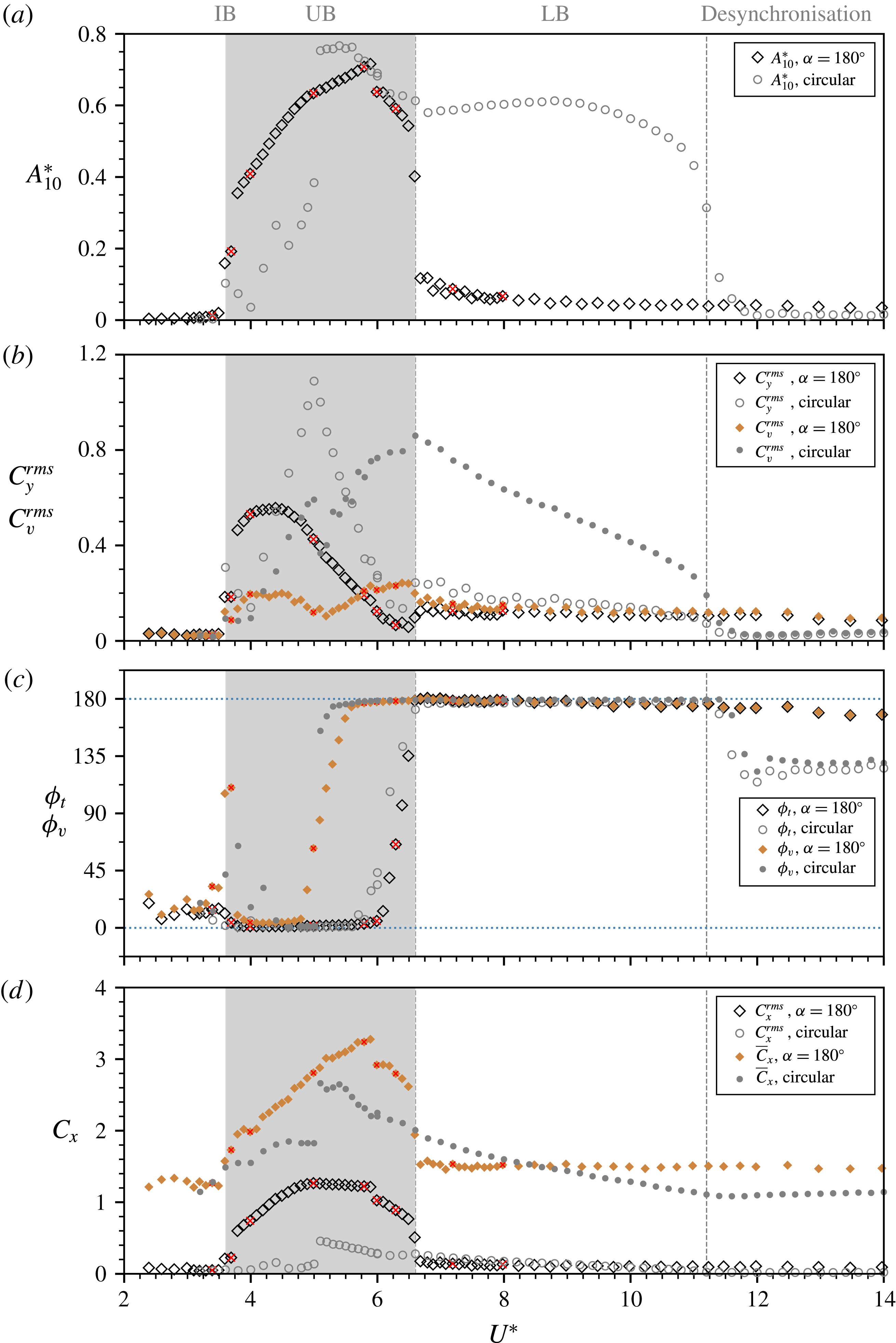
In this comparison, there are some remarkable similarities in several aspects between these two cases. At low reduced velocities, the onset of significant vibration occurs similarly from $U^{\ast }=3.6$ . Although lock-in occurs much earlier than the circular cylinder case, the reverse D-section sees its $A_{10}^{\ast }$ response in an increasing trend similar to that of the initial branch of the circular cylinder case for $3.6<U^{\ast }<5.0$ . The peak amplitude ( $A_{10}^{\ast }\simeq 0.72$ ) of the reverse D-section is found to be surprisingly comparable to that ( $A_{10}^{\ast }\simeq 0.77$ ) of the circular cylinder case, and they occur at similar reduced velocities near the middle of the upper branch (UB) of the circular cylinder case. Moreover, similar trends in variation with $U^{\ast }$ are seen in the fluid force coefficients (figure 11 b,d). Of further interest are the similar jumps from $0^{\circ }$ to $180^{\circ }$ in both $\unicode[STIX]{x1D719}_{t}$ (at $U^{\ast }\approx 5.0$ ) and $\unicode[STIX]{x1D719}_{v}$ (at $U^{\ast }=6.6$ ), which are indicative of pure VIV response. Furthermore, the dynamic response in the desynchronisation regime also appears to be highly similar to that of the circular cylinder case. From this comparison, it is evident that the reverse D-section can exhibit substantial vibration over a significant $U^{\ast }$ range where the initial and upper branches occur in the circular cylinder case. However, due to the lack of an afterbody, the vibration amplitude is attenuated by desynchronised fluid–structure interaction to very low values ( $A_{10}^{\ast }<0.1$ ) in the regime where the circular cylinder exhibits a lower branch; in other words, the lower branch of a circular cylinder is strongly related to its afterbody.

Perhaps surprisingly, the vortex shedding mode seen in all PIV measurements indicated in figure 11 was found to be 2S. This is unexpected, as previous studies on circular cylinders (e.g. Govardhan & Williamson Reference Govardhan and Williamson2000; Zhao et al. Reference Zhao, Leontini, Lo Jacono and Sheridan2014a ) have shown that different wake mode transitions are associated with jumps in $\unicode[STIX]{x1D719}_{t}$ and $\unicode[STIX]{x1D719}_{v}$ from $0^{\circ }$ to $180^{\circ }$ . To clarify the present findings, figure 12 shows sample time traces at four selected locations from different vibration regimes: $(a)$   $U^{\ast }=3.4$ , where extremely small vibration amplitude is observed and both $\unicode[STIX]{x1D719}_{t}$ and $\unicode[STIX]{x1D719}_{v}$ fluctuate around $0^{\circ }$ for most of the time duration; $(b)$   $U^{\ast }=4.0$ in the early lock-in stage, where significant vibration is encountered, and with both $\unicode[STIX]{x1D719}_{t}$ and $\unicode[STIX]{x1D719}_{v}$ still remaining around $0^{\circ }$ ; $(c)$   $U^{\ast }=6.0$ , where large oscillations are encountered with $\unicode[STIX]{x1D719}_{t}$ fluctuating around $0^{\circ }$ and $\unicode[STIX]{x1D719}_{v}$ fluctuating around $180^{\circ }$ ; and $(d)$   $U^{\ast }=8.0$ in the desynchronisation region, where the vibration amplitude is attenuated to very low values with both $\unicode[STIX]{x1D719}_{t}$ and $\unicode[STIX]{x1D719}_{v}$ fluctuating slightly around $180^{\circ }$ . Figure 13 presents the observed 2S wake mode at selected reduced velocities $U^{\ast }=4.0$ , $6.0$ and $8.0$ . As can be seen, vortices are shed directly from the trailing edges of the D-section at both maximum and minimum positions (see corresponding supplementary movies for full vortex shedding cycles). These results suggest that the afterbody plays an important role affecting the wake structure. They show that the vortex shedding mode may not necessarily be related to $\unicode[STIX]{x1D719}_{t}$ and $\unicode[STIX]{x1D719}_{v}$ , as for VIV of circular and ‘diamond-shaped’ (square cross-section placed at $45^{\circ }$ flow incidence angle) cylinders that possess an afterbody (see Zhao et al. Reference Zhao, Leontini, Lo Jacono and Sheridan2014a ,Reference Zhao, Leontini, Lo Jacono and Sheridan b ).

Figure 12.

Sample time traces of the cylinder vibration for $\unicode[STIX]{x1D6FC}=180^{\circ }$ at different reduced velocities: (a) $U^{\ast }=3.4$ , (b) $U^{\ast }=4.0$ , (c) $U^{\ast }=6.0$ and (d) $U^{\ast }=8.0$ . For more details, see the caption of figure 5.

Figure 13.

Phase-averaged vorticity contours showing 2S patterns at $U^{\ast }=4.0$ , $6.0$ and $8.0$ in columns (a), (b) and (c), respectively, for $\unicode[STIX]{x1D6FC}=180^{\circ }$ . For more details, refer to the caption of figure 6. See supplementary movies 9–11 for the full oscillation cycles.

3.2.3 Analysis of galloping instability using quasi-steady approach

In this section, the potential for galloping based on quasi-steady theory is assessed for the two $\unicode[STIX]{x1D6FC}$ cases by evaluating the transverse lift force acting on the ‘static’ body with varying relative angle of attack ( $\unicode[STIX]{x1D6FC}^{\prime }$ ). This quasi-steady approach is based on the assumption that the fluid force is in phase with the body velocity and the instantaneous driving force acting on the moving body is nearly equal to the static force evaluated at the instantaneous angle of flow incidence (Naudascher & Rockwell Reference Naudascher and Rockwell2005).

Figure 14.

The mean lift and drag coefficients as a function of the relative angle of attack in (a,b) and the $\unicode[STIX]{x1D6FD}$ variation in (c) for the orientation case of $\unicode[STIX]{x1D6FC}=0^{\circ }$ at $Re=4880$ . The solid lines in (a,b) represent the third-order polynomial fitting curves. In (c), the dashed line represents $|\unicode[STIX]{x2202}C_{L}/\unicode[STIX]{x2202}\unicode[STIX]{x1D6FC}^{\prime }|$ . Note that $\unicode[STIX]{x1D6FC}^{\prime }$ is increased in the clockwise direction.

Figure 15.

The mean lift and drag coefficients as a function of the relative angle of attack in (a,b) and the $\unicode[STIX]{x1D6FD}$ variation in (c) for the orientation case of $\unicode[STIX]{x1D6FC}=0^{\circ }$ at $Re=4880$ . For more details, see the caption of figure 14.

Based on (2.1), the governing equation of the cylinder motion can be rewritten as

(3.1) $$\begin{eqnarray}m\ddot{y} +2m\unicode[STIX]{x1D701}_{n}\unicode[STIX]{x1D714}_{n}{\dot{y}}+m\unicode[STIX]{x1D714}_{n}^{2}y={\textstyle \frac{1}{2}}\unicode[STIX]{x1D70C}U^{2}DLC_{y},\end{eqnarray}$$

where $\unicode[STIX]{x1D701}_{n}$ is the structural damping ratio and $\unicode[STIX]{x1D714}_{n}=2\unicode[STIX]{x03C0}f_{n}$ the natural angular frequency of the system in vacuum. (Note that these parameters are assumed to be very nearly equal to those determined through free-decay test in air in the present study.) According to the quasi-steady theory developed by Parkinson & Smith (Reference Parkinson and Smith1964), the driving force can be expressed as

(3.2) $$\begin{eqnarray}C_{y}=\mathop{\sum }_{j=1}^{\infty }a_{j}\left(\frac{{\dot{y}}}{U}\right)^{j}=a_{1}\frac{{\dot{y}}}{U}+a_{2}\left(\frac{{\dot{y}}}{U}\right)^{2}+a_{3}\left(\frac{{\dot{y}}}{U}\right)^{3}+\cdots \,,\end{eqnarray}$$

where $a_{j}$ is the $j$ th polynomial coefficient. By considering only small-amplitude disturbances to the system (Blevins Reference Blevins1990; Naudascher & Rockwell Reference Naudascher and Rockwell2005), equation (3.1) can be approximated by

(3.3) $$\begin{eqnarray}C_{y}=a_{1}\frac{{\dot{y}}}{U}.\end{eqnarray}$$

Substituting (3.3) for (3.1) gives

(3.4) $$\begin{eqnarray}\ddot{y} +\left(2\unicode[STIX]{x1D701}_{n}\unicode[STIX]{x1D714}_{n}-\frac{1}{2m}\unicode[STIX]{x1D70C}UDLa_{1}\right){\dot{y}}+\unicode[STIX]{x1D714}_{n}^{2}y=0.\end{eqnarray}$$

The term in parentheses in this equation is the net damping factor as the sum of the structural and aerodynamic components. The system is stable if the net damping factor is larger than zero. Thus, the critical flow velocity for possible onset of galloping can be evaluated by

(3.5) $$\begin{eqnarray}U_{cr}=\frac{4m\unicode[STIX]{x1D701}_{n}\unicode[STIX]{x1D714}_{n}}{\unicode[STIX]{x1D70C}DLa_{1}}=\frac{4m\unicode[STIX]{x1D701}_{n}(2\unicode[STIX]{x03C0}f_{na})}{\unicode[STIX]{x1D70C}DLa_{1}},\end{eqnarray}$$

and the critical reduced velocity by

(3.6) $$\begin{eqnarray}U_{cr}^{\ast }=\frac{U_{cr}}{f_{nw}D}=\frac{4m\unicode[STIX]{x1D701}_{n}(2\unicode[STIX]{x03C0}f_{na})}{\unicode[STIX]{x1D70C}DLa_{1}(f_{nw}D)}=\frac{\unicode[STIX]{x03C0}^{2}m^{\ast }\unicode[STIX]{x1D701}_{n}}{a_{1}}\left(\frac{f_{na}}{f_{nw}}\right).\end{eqnarray}$$

According to the criterion of transverse galloping given by Den Hartog (Reference Den Hartog1932, Reference Den Hartog1956), a system with no structural damping is potentially unstable if

(3.7) $$\begin{eqnarray}\unicode[STIX]{x1D6FD}=\frac{\unicode[STIX]{x2202}C_{y}}{\unicode[STIX]{x2202}\unicode[STIX]{x1D6FC}^{\prime }}=-\frac{\unicode[STIX]{x2202}C_{L}}{\unicode[STIX]{x2202}\unicode[STIX]{x1D6FC}^{\prime }}-C_{D}>0,\end{eqnarray}$$

where $C_{L}$ is the lift coefficient acting perpendicularly to the relative flow ( $U_{rel}=\sqrt{U^{2}+{\dot{y}}^{2}}$ ) and $C_{D}$ is the drag coefficient parallel to the relative flow. Figures 14 and 15 show the mean lift ( $\overline{C}_{L}$ ) and drag ( $\overline{C}_{D}$ ) coefficients as a function of the relative angle of attack $\unicode[STIX]{x1D6FC}^{\prime }$ , together with the $\unicode[STIX]{x1D6FD}=\unicode[STIX]{x2202}C_{y}/\unicode[STIX]{x2202}\unicode[STIX]{x1D6FC}^{\prime }$ variation for the two orientation cases of $\unicode[STIX]{x1D6FC}=0^{\circ }$ and $180^{\circ }$ , respectively. Note that the measurements were conducted at a representative Reynolds number $Re=4880$ (corresponding to $U^{\ast }=10$ close to the middle of the $U^{\ast }$ range tested in the FIV cases). The polynomial coefficient $a_{1}$ in (3.2) is given by $a_{1}=\unicode[STIX]{x1D6FD}|_{\unicode[STIX]{x1D6FC}^{\prime }=0^{\circ }}$ . Thus, in theory, $U_{cr}^{\ast }$ can be determined using (3.6) for the two $\unicode[STIX]{x1D6FC}$ cases.

As can be seen from figure 14, $a_{1}=\unicode[STIX]{x1D6FD}|_{\unicode[STIX]{x1D6FC}^{\prime }=0^{\circ }}\simeq 0.13$ is slightly positive, which implies that the D-section is potentially susceptible to galloping with respect to soft excitation (from rest) in the present study, as has been confirmed by the structural vibration response shown in § 3.1. Note that there are some differences between measured values of $\unicode[STIX]{x1D6FD}|_{\unicode[STIX]{x1D6FC}^{\prime }=0^{\circ }}$ previously reported in the literature. For example, Harris (Reference Harris1948) found that the D-section was unstable, Cheers (Reference Cheers1950) found that $\unicode[STIX]{x1D6FD}$ was small and negative, while Brooks (Reference Brooks1960) reported that $\unicode[STIX]{x1D6FD}$ remained very close to zero for $\unicode[STIX]{x1D6FC}^{\prime }$ up to $25^{\circ }$ , suggesting that Den Hartog’s criterion was not satisfied and thus the D-section should not gallop from rest. The value of $\unicode[STIX]{x1D6FD}|_{\unicode[STIX]{x1D6FC}^{\prime }=0^{\circ }}$ is also slightly different from that of previous studies conducted at higher Reynolds numbers (e.g.  $Re=9\times 10^{4}$ in Novak & Tanaka (Reference Novak and Tanaka1974), and $Re=8.2\times 10^{4}$ in Weaver & Veljkovic (Reference Weaver and Veljkovic2005)) where the $C_{y}$ versus $\unicode[STIX]{x1D6FC}^{\prime }$ curve exhibited a zero or very small value with a negative slope at $\unicode[STIX]{x1D6FC}^{\prime }=0^{\circ }$ , and an initial amplitude was thereby required to trigger a hard galloping response. These discrepancies are thus likely to be mostly attributable to a difference in $Re$ , although other factors (e.g. the flow turbulence level) may also play a role. In any case, $\unicode[STIX]{x1D6FD}$ is a small difference between two relatively much larger terms: the lift curve slope ( ${\sim}-2.7$ ) and the damping due to drag ( ${\sim}2.6$ ). Thus, small variations in either of these terms will alter whether soft galloping will occur according to the Den Hartog criterion.

On the other hand, given $a_{1}\simeq 0.13$ from figure 14, the (critical) onset reduced velocity for galloping response is evaluated using (3.6) to be $U_{cr}^{\ast }\simeq 0.73$ . Apparently, this $U_{cr}^{\ast }$ value is much lower than the reduced velocity expected for VIV resonance, $U_{r}^{\ast }=1/St\simeq 7.1$ . In fact, negligible structural vibration is observed prior to the VIV resonance occurring at $U^{\ast }=3.0$ (or $0.42U_{r}^{\ast }$ ) in the present experiments. This phenomenon seems to be due to the so-called ‘quenching effect’ of the vortex system on the galloping instability as explained by Corless & Parkinson (Reference Corless and Parkinson1988). However, the galloping-dominated response observed in the experiments occurs at reduced velocities higher than $1.76U_{r}^{\ast }$ . Of course, at very low $U^{\ast }$ , the vortex shedding period is very long compared with the natural system oscillation period, so the use of the mean lift variation with incidence angle derived from averaging the effect of shedding over many cycles is not a reasonable approximation. One would expect that this approximation should only become reasonable well beyond the resonant reduced velocity of $U^{\ast }=1/St=7.1$ . Interestingly, in this case, the lift curve slope remains strongly negative to high incidence angles, which is also qualitatively consistent with large galloping oscillations.

For a particular $U^{\ast }$ , assuming that the body is oscillating at the natural frequency, the amplitude variation can be approximated as a sinusoidal variation, i.e.

(3.8) $$\begin{eqnarray}y/D=(A/D)\sin (2\unicode[STIX]{x03C0}f_{nw}t).\end{eqnarray}$$

Differentiating this gives

(3.9) $$\begin{eqnarray}\frac{{\dot{y}}}{U}~(=\tan \unicode[STIX]{x1D6FC}^{\prime })=\frac{2\unicode[STIX]{x03C0}(A/D)Df_{nw}}{U}\cos (2\unicode[STIX]{x03C0}f_{nw}t)\quad \Rightarrow \quad \unicode[STIX]{x1D6FC}_{max}^{\prime }=\tan ^{-1}\left(\frac{2\unicode[STIX]{x03C0}A^{\ast }}{U^{\ast }}\right).\end{eqnarray}$$

Taking the value of $A/D=4.7$ at $U^{\ast }=20$ , where the body is still undergoing strong galloping, gives $\unicode[STIX]{x1D6FC}_{max}^{\prime }\simeq 55^{\circ }$ , i.e. as the body moves past its equilibrium position, the flow incidence angle seen by the body is $55^{\circ }$ . This indicates that galloping does occur over a wide range of angles of attack, extending a long way from $\unicode[STIX]{x1D6FC}^{\prime }=0^{\circ }$ .

For the reversed-D case of $\unicode[STIX]{x1D6FC}=180^{\circ }$ shown in figure 15, $\unicode[STIX]{x1D6FD}$ is found to be $-1.81$ at $\unicode[STIX]{x1D6FC}^{\prime }=0$ , which is considerably lower than the reported value of $-1.15$ for high- $Re$ wind-tunnel experiments (Cheers Reference Cheers1950), and it remains significantly negative over the $\unicode[STIX]{x1D6FC}^{\prime }$ range tested. Both the lift slope and the drag contribute to damping in this case. This implies that the reversed D-section is not susceptible to a soft galloping instability, which is consistent with the observed response over the entire reduced velocity range investigated.

In summary, the quasi-steady theory predicts that soft galloping will occur for the D-section but not the reversed D-section, consistent with the experimental results. Perhaps also of interest is that the critical reduced velocity for galloping is proportional to $m^{\ast }$ through (3.6), hence the onset values for galloping in air will typically be very much greater than the calculated values here (for water), placing the onset of galloping beyond the $U^{\ast }$ range for VIV. This may result in cleaner physical behaviour with a greater separation between the underlying physical processes causing the different forms of FIV.