Optimal design of photoreceptor mosaics: Why we do not see color at night

JEREMY R. MANNING; DAVID H. BRAINARD

doi:10.1017/S095252380808084X

Optimal design of photoreceptor mosaics: Why we do not see color at night

Published online by Cambridge University Press: 01 January 2009

JEREMY R. MANNING and

DAVID H. BRAINARD

Show author details

JEREMY R. MANNING*: Affiliation:
Neuroscience Graduate Group and Department of Psychology, University of Pennsylvania, Philadelphia, Pennsylvania
DAVID H. BRAINARD*: Affiliation:
Neuroscience Graduate Group and Department of Psychology, University of Pennsylvania, Philadelphia, Pennsylvania
*: *Address correspondence and reprint requests to: David H. Brainard, 3401 Walnut Street, Philadelphia, PA 19104. E-mail: brainard@psych.upenn.edu

Article contents

Abstract
Introduction
General formulation
Simplified formulation
Results
Discussion
Footnotes
References

Rights & Permissions

Abstract

While color vision mediated by rod photoreceptors in dim light is possible (Kelber & Roth, 2006), most animals, including humans, do not see in color at night. This is because their retinas contain only a single class of rod photoreceptors. Many of these same animals have daylight color vision, mediated by multiple classes of cone photoreceptors. We develop a general formulation, based on Bayesian decision theory, to evaluate the efficacy of various retinal photoreceptor mosaics. The formulation evaluates each mosaic under the assumption that its output is processed to optimally estimate the image. It also explicitly takes into account the statistics of the environmental image ensemble. Using the general formulation, we consider the trade-off between monochromatic and dichromatic retinal designs as a function of overall illuminant intensity. We are able to demonstrate a set of assumptions under which the prevalent biological pattern represents optimal processing. These assumptions include an image ensemble characterized by high correlations between image intensities at nearby locations, as well as high correlations between intensities in different wavelength bands. They also include a constraint on receptor photopigment biophysics and/or the information carried by different wavelengths that produces an asymmetry in the signal-to-noise ratio of the output of different receptor classes. Our results thus provide an optimality explanation for the evolution of color vision for daylight conditions and monochromatic vision for nighttime conditions. An additional result from our calculations is that regular spatial interleaving of two receptor classes in a dichromatic retina yields performance superior to that of a retina where receptors of the same class are clumped together.

Keywords

Photoreceptor mosaic Color vision Nocturnal vision Bayesian decision theory Retina

Information

Type: Natural Scene Statistics and Efficient Coding
Information: Visual Neuroscience , Volume 26 , Issue 1 , January 2009 , pp. 5 - 19

DOI: https://doi.org/10.1017/S095252380808084X [Opens in a new window]
Copyright: Copyright © Cambridge University Press 2009

Introduction

The vertebrate retina contains two broadly distinguished classes of photoreceptors, rods and cones. Rods are characterized by low noise (Barlow, Reference Barlow1956; Baylor et al., Reference Baylor, Nunn and Schnapf1984; Schneeweis & Schnapf, Reference Schneeweis and Schnapf2000) and are effective at low light levels when photons are scarce. On the other hand, they saturate more easily than cones and their contribution to vision diminishes under daylight conditions (Aguilar & Stiles, Reference Aguilar and Stiles1954; Tamura et al., Reference Tamura, Nakatani and Yau1989; Demontis et al., Reference Demontis, Bisti and Cervetto1993; Burns & Arshavsky, Reference Burns and Arshavsky2005; Yin et al., Reference Yin, Smith, Sterling and Brainard2006). Cones are noisier than rods (Schnapf et al., Reference Schnapf, Nunn, Meister and Baylor1990; Rieke & Baylor, Reference Rieke and Baylor2000; Fu et al., Reference Fu, Kefalov, Luo, Xue and Yau2008) but operate without saturation at much higher light levels (Schneeweis & Schnapf, Reference Schneeweis and Schnapf1999). Cones are useful for daylight vision, when there is plenty of light. Across species, the relative numbers of rods and cones vary enormously, with nocturnal animals generally having a higher rod-to-cone ratio than diurnal animals (Walls, Reference Walls1942).

Within the rod and cone systems, there is additional across-species variability. Most vertebrates have multiple classes of cones, distinguished primarily by different spectral sensitivities. The presence of multiple cone classes enables color vision, as the relative responses of cones of different classes provide information about the relative spectrum of the incident light. Across species that have multiple classes of cones, there are additional variations. These include the number of distinct classes of cones present (Walls, Reference Walls1942; Jacobs, Reference Jacobs1981), the spectral sensitivities of the individual cone classes (Bowmaker, Reference Bowmaker, Cronly-Dillon and Gregory1991; Jacobs, Reference Jacobs1996; Jacobs & Rowe, Reference Jacobs and Rowe2004), and the pattern of how the cones are arranged in the retinal mosaic (Scholes, Reference Scholes1975; Wassle & Riemann, Reference Wassle and Riemann1978; Bowmaker & Kunz, Reference Bowmaker and Kunz1987; Mollon & Bowmaker, Reference Mollon and Bowmaker1992; Hofer et al., Reference Hofer, Carroll, Neitz, Neitz and Williams2005). A small minority of mammalian species that operate in low-light conditions have only one spectral class of cone (Jacobs et al., Reference Jacobs, Neitz and Neitz1996) and are thus monochromats under cone-mediated viewing conditions.

In contrast, most vertebrates have only a single class of rod. With only a single class of rod, variation in image intensity is perfectly confounded with variation in image relative spectrum, so that vision mediated by a single class of rod is monochromatic. The restriction to a single class is not due to any fundamental biophysical constraint, as a few species (e.g., the nocturnal hawkmoth, Deilephila elpenor) do have retinas with multiple classes of rods and have been shown behaviorally to have color vision at rod-mediated light levels (Kelber & Roth, Reference Kelber and Roth2006).

Previous authors have speculated about why color vision is rare at night. Walls (Reference Walls1942), for example, indicates that color vision could only be useful under conditions where spatial and contrast acuity are high and that it would not be useful when photons are scarce. Rushton (Reference Rushton1962) makes a similar statement. To our reading, however, neither of these authors offer reasoning to support their assertions. Moreover, it is now known that some plants and bacteria detect light with low spatial resolution but nonetheless have color vision (Skorupski & Chittka, Reference Skorupski and Chittka2008), in apparent contradiction to Walls’ and Rushton’s hypothesis. Also note that human rod-mediated visual acuity at approximately 5–10 deg eccentricity exceeds cone-mediated visual acuity at 40–50 deg eccentricity (Weymouth, Reference Weymouth1958, who replots data from Fick), again suggesting that factors other than those that limit resolution contribute to whether a retina should be monochromatic or not.

Land and Osorio (Reference Land and Osorio2003) articulate what we take, based on an informal polling of our colleagues, to be the standard intuition on this topic. This intuition starts with the observation that color vision depends on the difference between the responses of two receptor classes. The magnitude of this difference signal will on average be smaller than that of a luminance signal that arises from the sum of responses of the two classes or from a single receptor class.Footnote ¹ At the same time, the net effect of photon and dark noise is the same for both difference and summed signals. Thus, the idea is that color vision becomes less useful at low light levels because overall signal-to-noise drops, and noise swamps the output of an opponent color channel before it swamps that of a luminance channel. A related idea was formalized by van Hateren (Reference van Hateren1993), who showed that as signal-to-noise drops, optimal postreceptoral processing favors a luminance channel over a chromatic channel.

Note, however, that neither the standard intuition nor van Hateren’s (Reference van Hateren1993) calculations lead immediately to the conclusion that monochromatic vision is superior to color vision at low signal-to-noise. To do so requires an analysis that shows not just that the value of color vision decreases with light level but that a change to monochromatic vision leads to improved performance. That is, the fact that a luminance channel carries more information than an opponent color channel tells us neither that a monochromatic retina is superior to one with multiple receptor types nor that it is not advantageous to add a color-opponent channel to a luminance channel.

Barlow (Reference Barlow1957) argued that the spontaneous photopigment isomerization rate of photoreceptors might depend strongly on their wavelength of maximal sensitivity, with maximal sensitivity at shorter wavelengths leading to lower noise. This effect would be expected to occur for fundamental biophysical reasons: short-wavelength quanta have more energy than long-wavelength quanta, and this in turn would allow photopigments sensitive to short-wavelength quanta to have higher energy barriers for isomerization and be more resistant to thermal fluctuations (Platt, Reference Platt1956). Barlow argued that the overall shift in human visual sensitivity toward shorter wavelengths between cone- and rod-mediated vision (the Purkinje shift) maximizes absolute sensitivity by minimizing thermal noise. Barlow did not explicitly address trade-offs between color and monochromatic vision. However, his observation that the dependence of dark noise on spectral sensitivity has important implications for differences between daylight and nighttime vision plays a key role in the analysis we present below. Other closely related antecedents to the current paper are a treatment of the design of trichromatic mosaics (Garrigan et al., Reference Garrigan, Ratliff, Klein, Sterling, Brainnard and Balasubramanian2006, Reference Garrigan, Ratliff, Klein, Sterling, Brainard and Balasubramanian2008) and a treatment of optimal choice of cone spectral sensitivities (Lewis & Zhaoping, Reference Lewis and Zhaoping2006); these authors used an information-theoretic approach and emphasized the central role played by asymmetries in the information available at different wavelengths. We return in the discussion to review measurements of photoreceptor thermal noise.

Here we assess the efficacy of various choices of the design of the photoreceptor mosaic, in the context of the vertebrate eye. We formulate the design question in terms of an explicit model that defines optimal performance with respect to a specified statistical ensemble of stimuli. Our model allows us to calculate how well an ideal observer could estimate the incident image from the photoreceptor responses, and we examine how optimal performance varies with different aspects of eye design. Although our formulation is very general, we focus here on the performance trade-off between dichromatic (two receptor classes) and monochromatic (one receptor class) vision and how this interacts with overall light level. To address this question, our work also touches on other aspects of mosaic design. These include choice of photopigment spectral sensitivity and the packing arrangement of the mosaic.

In the next section, we introduce a general formulation. To make computational progress, however, we then make a number of simplifying assumptions. These include restricting attention to a model environment in which there are just two discrete wavelengths and where all images are characterized by the power in each wavelength at discrete image locations on a line (one spatial dimension.) We consider image ensembles characterized by Gaussian distributions, evaluate image estimation using a mean squared error criterion, and do not take into account the energetic cost of computation. Although a priori it might appear that these simplifying choices reduce the complexity of the model too severely, the simplified model is surprisingly rich, and studying it leads to interesting insight.

General formulation

We start with a general formulation. We model the visual environment as an ideal image, which specifies the intensity of light incident on the eye as a function of two angular spatial dimensions (x and y) and one spectral dimension (λ). For simplicity, we consider the case where each of these dimensions has been finely discretized. Thus, the ideal image is specified as I(x_i, y_j, λ_k). Note that in most three-dimensional scenes, the retinal image is not formed by viewing a planar ideal image. Rather, light reflects to the eye from objects located at various distances. The ideal image should be conceived as one that would produce the same retinal image as the actual illuminated objects in the scene.

Light from the ideal image passes through an optical apparatus consisting of a cornea, pupil, and lens. Refraction at the interfaces between the optical elements creates an image on the retina. Aberrations in the optics combine with diffraction to blur the retinal image; the blurring may be characterized by the point spread function of the optics. In general, the point spread function varies with wavelength because of chromatic aberration. It also depends on the pupil area ${\Bbb A}$ . In the typical regime where effects of optical aberrations dominate effects of diffraction, increasing pupil size increases both the intensity of the retinal image and the degree to which it is blurred.

We denote the point spread function by $P_{\Bbb A} (x_i ,y_j ,\lambda _k )$ , where ${\Bbb A}$ is the pupil area. It specifies the spread of light in the retinal image from a point source, and we assume it to be independent of the location of that source. The subscript ${\Bbb A}$ denotes the fact that the shape of the point spread function depends on pupil area. The retinal image may be computed as the convolution of the ideal image and the point spread function:

$R(x_i ,y_j ,\lambda _k ) = {\Bbb A}[I(x_i ,y_j ,\lambda _k ) \ast P_{\Bbb A} (x_i ,y_j ,\lambda _k )].$

By convention, $P_{\Bbb A} (x_i ,y_j ,\lambda _k )$ , is normalized to have unit volume; the effect of pupil area on overall light level is accounted for explicitly in the equation above.

The retinal image is sampled by an interleaved array of photoreceptors, with one photoreceptor at each location. The photopigment isomerization rates of each photoreceptor are the information about the image available to the visual system. We model the relation between the retinal image and the mean isomerization rate of a single photoreceptor of class l centered at location (x_m, y_n):

$\mu _l = \sum\limits_k^\ {([R(x_i ,y_j ,\lambda _k) \ast Y_l (x_i ,y_j)]|_{(x_m ,y_n)})S_l (\lambda _k)} + d_l .$

Here Y_l(x_i, y_j) represents the acceptance aperture of the l ^th photoreceptor class, S_l(λ_k) represents the spectral sensitivity of the l ^th class, and d_l represents the mean number of spontaneous isomerizations per second of the i ^th class. The actual number of isomerizations in response to an image shown for a duration Δt is distributed as a Poisson process with mean (μ_lΔt). We take the task of visual processing as estimating the ideal image from the noisy array of photoreceptor responses. At this juncture, it is convenient to express the ideal image, which consists of a finite array of intensities, as a vector $\vec i$ . The estimator may then be expressed as

$\hat i = F(\vec r),$

where $\hat i$ is the estimate of $\vec i$ and $\vec r$ is a vector representing the entire array of noisy responses. The appropriate estimator F( ) depends on the exact design properties of the model visual system, on the statistical ensemble of images that will be encountered, on a loss function that describes how bad it is to approximate any given ideal image with any particular estimate, and on a decision about how loss should be aggregated over the statistical image ensemble. Once choices for each of these factors are made, however, the estimator F() can be chosen to optimize aggregate performance. Moreover, we can use optimized aggregate performance as a metric to ask which eye design parameters are best.

To construct an optimal estimator, we turn to Bayesian decision theory (Blackwell & Girschick, Reference Blackwell and Girschick1954; Berger, Reference Berger1985; Gelman et al., Reference Gelman, Carlin, Stern and Rubin2004). We start by expressing the relation between the ideal image and noisy response vector as a probability distribution $P(\vec r|\vec i)$ . This is called the likelihood and represents how probable any response vector is, conditional on knowing the ideal image.

The second step is to express the statistical structure of the environment as a probability distribution, $P(\vec i)$ . This is called the prior. The prior captures what is known or assumed about stimuli in the model environment (here the ideal image), independent of the observed photoreceptor responses. Bayes’ rule then yields the posterior

$P(\vec i|\vec r) = {\Bbb C}P(\vec r|\vec i)P(\vec i),$

where ℂ is a normalizing constant. The posterior tells us how probable any particular image is, given the observed photoreceptor responses.

To obtain a particular estimate $\hat i$ from the posterior, we need to specify a loss function $L(\hat i,\vec i)$ . This function provides the cost of choosing any estimate $\hat i$ when the actual image is $\vec i$ . Once the loss function is given, we can define the Bayes’ risk (Berger, Reference Berger1985) of an estimator $F(\vec r)$ as

$R_F = \int_{\vec i} {\left[ {\int_{\vec r} {L(F(\vec r),\vec i)P(\vec r|\vec i){\rm{d}}\vec r} } \right]P(\vec i){\rm{d}}\vec i} .$

The Bayes’ risk provides the expected loss associated with repeated applications of the estimator, when the images leading to the responses are drawn from the prior distribution $P(\vec i)$ . To see this, note that the inner integral takes the expectation over responses $\vec r$ given the image $\vec i$ (according to the likelihood), while the outer integral takes the expectation over images (according to the prior). In the absence of any computational constraints, a widely used optimality principle is to choose the estimator F() that minimizes R_F. In the development below, however, we will use the notation O_F to denote the quantity to be minimized, with O_F = R_F. Although not immediately relevant, this change in notation reminds us that there are alternative possible formulations of optimality. For example, in the discussion, we briefly treat the possibility of including energetic cost in addition to performance.

Given a specified likelihood, prior, and loss function, denote by F ^opt() an estimator that minimizes O_F and by $O_F^{{\rm{opt}}}$ the corresponding minimized value. We refer to $O_F^{{\rm{opt}}}$ as the optimized error. The prior and loss function describe the features of the environment and organism that define the visual system design problem, while the likelihood function describes the visual system’s solution. That is, if we hold $P(\vec i)$ and $L(\hat i,\vec i)$ constant, we can regard $O_F^{{\rm{opt}}}$ as a function of the likelihood. The optimal design is then the one corresponding to the likelihood $P(\vec r|\vec i)$ that minimizes $O_F^{{\rm{opt}}} [P(\vec r|\vec i)]$ . This is the approach we implement below. At this level of generality, it closely parallels the approach used by Srinivasan et al. (Reference Srinivasan, Laughlin and Dubs1982) to consider the receptive fields of ganglion cells, as well as that developed recently by Levin et al. (Reference Levin, Durand and Freeman2008) in the context of evaluating the design of digital cameras.

Simplified formulation

To apply our general framework to mosaic design, and in particular to the trade-off between color and monochromatic vision, we make concrete simplifying assumptions. When the simplified version of the general model is able to predict observed biological design features, we gain insight about what properties of the environment are likely to have driven the evolution of these features. When the simplified version fails to predict the biology, we gain insight by considering ways in which the model is oversimplified or, alternatively, ways in which evolution has failed to arrive at an optimal design.

Image representation and prior

We start with one spatial dimension. Multi-wavelength–band images of this sort may be represented as column vectors:

$\eqalign{ \vec i =\ [ {m_{x_1 ,\lambda _1 } ,m_{x_2 ,\lambda _1 } , \ldots ,m_{x_{\Bbb I} ,\lambda _1 } ,m_{x_1 ,\lambda _2 } ,m_{x_2 ,\lambda _2 } , \ldots , }\cr m_{x_{\Bbb I} ,\lambda _2 } , \ldots ,m_{x_1 ,\lambda _{\Bbb K} } ,m_{x_2 ,\lambda _{\Bbb K} } , \ldots ,m_{x_{\Bbb I} ,\lambda _{\Bbb K} }]^{\text{T}},$

where $m_{x_i ,\lambda _k }$ is the intensity of wavelength λ_k at pixel i. We have $1 \leq i \leq {\Bbb I}$ and $1 \leq k \leq {\Bbb K}$ . For our calculations, we used 36 spatial locations and 2 wavelengths, so ${\Bbb I} = 36$ and ${\Bbb K} = 2$ .

Natural images are characterized by high correlations between the intensities at neighboring spatial locations (Pratt, Reference Pratt1978; Burton & Moorehead, Reference Burton and Moorehead1987; Field, Reference Field1987; Simonceli, Reference Simonceli and Bovik2005) and between intensities in the same location but at different wavelengths (Burton & Moorehead, Reference Burton and Moorehead1987; Ruderman et al., Reference Ruderman, Cronin and Chiao1998).Footnote ² These statistical features of natural images may be captured using a multivariate Gaussian distribution over multi-wavelength–band image vectors $\vec i:$

$P(\vec i) = N(\vec \mu _{{\rm{prior}}} ,{\bf K}_{{\rm{prior}}}),$

where $\vec \mu _{{\rm{prior}}}$ and K_prior are the mean and covariance matrix of the distribution, respectively. We required that $P(\vec i)$ be separable between space and wavelength, so that the spatial statistics were the same in each waveband, up to multiplicative scaling. In addition, we viewed the distribution $P(\vec i)$ as induced when a spatially uniform illuminant reflected from a set of surfaces, which allowed us to parametrically vary the intensity of the illuminant. For illuminant intensity ω and mean surface reflectances $\bar m_{\lambda _1 }$ and $\bar m_{\lambda _2 }$ at the two wavelengths, $\vec \mu _{{\rm{prior}}}$ was given by

$\vec \mu _{{\text{prior}}} = \omega \times [\bar m_{\lambda _1 } \times O(1,{\Bbb I}),\bar m_{\lambda _2 } \times O(1,{\Bbb I})]^{\text{T}},$

where O(a, b) is a matrix of 1s with a rows and b columns. The covariance matrix K_prior was given by the Kronecker product K_S ⊗ K_C, where K_S was the covariance matrix in the spatial domain and K_C was the covariance matrix in the wavelength domain.

We constructed K_S to represent a first-order Markov process (Pratt, Reference Pratt1978), so that

${\bf K}_S (u,v) = r_S^{(u - v)} ,$

where K_S(u, v) represents the entry in the u ^th row and v ^th column of K_S and r_S is the within-wavelength correlation between image intensities at neighboring locations. The use of a Markov model allowed us to adjust the correlational structure of the image ensemble with a single parameter and made more practical exploring how this structure affects optimal design.

We defined K_C as

${\bf K}_C = \omega ^2 \times \left[ {\matrix{ {\sigma _{\lambda _1 }^2 } & {r{_C}\sigma _{\lambda _1 } \sigma _{\lambda _2 } } \cr {r_C \sigma _{\lambda _1 } \sigma _{\lambda _2 } } & {\sigma _{\lambda _2 }^2 } \cr } } \right],$

where $\sigma _{\lambda _1 }$ is the standard deviation of reflectances at the first wavelength, $\sigma _{\lambda _2 }$ is the standard deviation of reflectances at the second wavelength, and r_C is the correlation (taken over locations) of the reflectances at the two wavelengths. This formulation for K_C could be easily generalized to ${\Bbb K} = 2$ wavelengths by treating it as representing a first-order Markov process over wavelength and regarding r_C as the correlation between neighboring wavelengths.

Image formation and likelihood

Given ${\Bbb I}$ pixels and ${\Bbb K}$ wavelengths, a render matrix R determines the responses of each of the ${\Bbb L} \leq {\Bbb I}$ photoreceptors in the modeled retina. The render matrix has ${\Bbb L}$ rows and ( ${\Bbb I} \;\times\; {\Bbb K}$ ) columns, where the value of the element in the u ^th row and v ^th column is the responsiveness of photoreceptor u to light at pixel ( $(v - 1)\% {\Bbb I}$ ) + 1 of wavelength $⌈{{v}\over{{\Bbb I}}}⌉$ . Here the symbol % represents the modulus operator.

To illustrate the idea, consider a retina with four evenly spaced photoreceptors that alternate between two classes, where each class is sensitive to only one wavelength. Suppose that there is no optical blurring and that each photoreceptor is sensitive to light from only one spatial location and one wavelength. Then, for an environment where there are eight spatial locations and two wavelengths, we would have

${\bi R} = \left[ {\matrix{ 0 & 1 & 0 & 0 & 0 & 0 & 0 & 0 \cr 0 & 0 & 0 & 0 & 0 & 0 & 0 & 0 \cr 0 & 0 & 0 & 0 & 0 & 1 & 0 & 0 \cr 0 & 0 & 0 & 0 & 0 & 0 & 0 & 0 \cr } \left| {\matrix{ 0 & 0 & 0 & 0 & 0 & 0 & 0 & 0 \cr 0 & 0 & 0 & 1 & 0 & 0 & 0 & 0 \cr 0 & 0 & 0 & 0 & 0 & 0 & 0 & 0 \cr 0 & 0 & 0 & 0 & 0 & 0 & 0 & 1 \cr } } \right.} \right].$

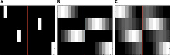
The first eight columns of this matrix represent the sensitivity of each photoreceptor to the first wavelength, while the second eight represent the sensitivity of each photoreceptor to the second wavelength. Rows 1 and 3 thus describe the first class of photoreceptor, and their spatial location is indicated by the column containing the 1. Rows 2 and 4 represent the second class of photoreceptor in a similar fashion. This render matrix is shown pictorially in Fig. 1A.

Fig. 1.

Three simple render matrices with varying optical blur and spectral sensitivity. In these examples, we show four photoreceptors, eight pixels, and two wavelengths. Each row corresponds to one photoreceptor. Columns to the left of the red line correspond to the first wavelength, while columns to the right correspond to the second wavelength. Within a wavelength, columns correspond to spatial locations. Darker areas correspond to lower sensitivity, while lighter areas correspond to higher sensitivity. (A) This render matrix corresponds to the example given numerically in the text, with each photoreceptor sensitive to incident light at a single punctate location and at a single wavelength. (B) Effect of optical blur. The standard deviation of the Gaussian used to compute optical blur was set to two pixels, and each photoreceptor is sensitive to one of the two wavelengths. (C) Spatial blur is the same as in B, but photoreceptors are 75% sensitive to one wavelength and 25% sensitive to the other. Each matrix shown was normalized to have the same maximum intensity for display.

Fig. 1B illustrates the addition of optical blurring to our four-photoreceptor example. Blurring was computed by centering a Gaussian at each photoreceptor’s position. Fig. 1C illustrates a render matrix for a retina containing photoreceptor sensitive to both wavelengths but to different degrees. The general formulation of the render matrix allows arbitrary spatial and wavelength sensitivity to be specified.

Given a render matrix R and a draw from the stimulus distribution, $\vec i$ , the photoreceptor responses to $\vec i$ are given by the ${\Bbb L}$ -element column vector $\vec r$ :

$\vec r = {\bf R}\vec i + \user{\varepsilon },$

where ε represents photoreceptor noise and was a draw from the Gaussian distribution $N(\vec \mu _{{\rm{noise}}} ,{\bf K}_{{\rm{noise}}})$ . For our simulations, we used an ${\Bbb L}$ -dimensional column vector as $\vec \mu _{{\rm{noise}}}$ , where the u ^th entry is given by the mean dark noise d_l of the photoreceptor represented by the u ^th row of the render matrix. The noise covariance matrix K_noise is an ${\Bbb L}$ × ${\Bbb L}$ diagonal matrix where the diagonal is given by $\omega \times \bar m_{\lambda _k } + d_l$ . With this choice of noise, the likelihood function was then given by the Gaussian

$P(\vec r|\vec i) = N({\bf R}\vec i + \vec \mu _{{\rm{noise}}} ,{\bf K}_{{\rm{noise}}}).$

We used a Gaussian approximation to the more realistic Poisson noise distribution so that we could leverage analytic results (see below) that apply for the Gaussian case.

Optimal estimator

Given the prior and likelihood, the optimal estimator depends on the loss function. The appropriate loss function for biological vision is almost certainly a highly complicated function of the image and the estimate, as some estimation errors will have much more serious consequences for survival and reproduction than others. Nonetheless, for practical reasons, we simplify in the remainder of the paper by restricting attention to a simple squared error loss function 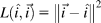$L(\hat i,\vec i) = \left\| {\vec i - \hat i} \right\|^2$ . Although this loss function does not fully capture the biologically relevant aspects of estimation error, it has the feature that the estimator that minimizes the corresponding R_F is the mean of the posterior distribution.

Our prior and likelihood distributions are multivariate Gaussian with known mean and covariance. Therefore, the posterior is also multivariate Gaussian, and its mean and covariance may be computed in closed form (Gelman et al., Reference Gelman, Carlin, Stern and Rubin2004). The estimated image $\hat i$ is given by:

$\hat i = \vec \mu _{{\rm{posterior}}} = {\bf F}\vec r + \vec i_0 ,\;{\rm{where}}$

${\bf F} = {\bf K}_{{\rm{prior}}} {\bf R}^{\rm{T}} ({\bf RK}_{{\rm{prior}}} {\bf R}^{\rm{T}} + {\bf K}_{{\rm{noise}}} )^{ - 1} \;{\rm{and}}$

$\vec i_0 = \vec \mu _{{\rm{prior}}} - {\bf FR}\vec \mu _{{\rm{prior}}} - {\bf F}\vec \mu _{{\rm{noise}}}.$

Moreover, for our choice of squared error loss, $O_F^{{\rm{opt}}} [P(\vec r|\vec i)]$ is given by the trace of the posterior covariance matrix:

$O_F^{{\rm{opt}}} [P(\vec r|\vec i)] = {\rm{trace}}({\bf K}_{{\rm{posterior}}} ),\;{\rm{where}}$

${\bf K}_{{\rm{posterior}}} = {\rm{(}}{\bf K}_{{\rm{prior}}}^{ - 1} + {\bf R}^{\rm{T}} {\bf K}_{{\rm{noise}}}^{ - 1} {\bf R}{\rm{)}}^{ - {\rm{1}}} {\rm{.}}$

Results

Color versus monochromatic vision at high illumination levels

We begin by comparing the performance of dichromatic and monochromatic vision at a high illumination level. Consider two fixed classes of photoreceptor, with class 1 expressing photopigment sensitive only to wavelength λ ₁ and class 2 expressing photopigment sensitive only to wavelength λ ₂. We assume that the mean and variance of the image are the same for the two wavelengths and that the two classes of photoreceptors have the same dark noise. These choices make the model environment and visual system symmetric with respect to wavelength. To mimic the statistical structure of natural images, we choose high values for the spatial and wavelength correlations: r_S was set to 0.9 and r_C was set to 0.8. We fixed the optical blur (Gaussian with standard deviation of two pixels), photoreceptor aperture (three pixels), illumination level (ω = 2000), and dark noise of each photoreceptor class (d ₁ = d ₂ = 1). These choices lead to a good signal-to-noise ratio (SNR) in individual photoreceptors. To see this, note that receptor SNR is given by

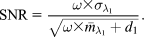
${\rm{SNR}} = {{\omega \times \sigma _{\lambda _1 } } \over {\root \of {\omega \times \bar m_{\lambda _1 } + d_1 } }}.$

Here, SNR = 44.7 or 16.5 dB.

To compare dichromatic and monochromatic vision, we computed $O_F^{{\rm{opt}}}$ for all 4096 possible regularly spaced arrays of 12 photoreceptors on a 36-pixel line. Two of these arrangements, one with all class 1 receptors and the other with all class 2 receptors, represent monochromatic vision. The other 4094 arrangements represent dichromatic vision with varying choices of class 1 to class 2 receptor ratio and with various arrangements of the two classes. The question we asked was, which mosaic arrangement leads to the minimum value of $O_F^{{\rm{opt}}}$ ? The answer is that an alternating array of class 1 and class 2 receptors, corresponding to dichromatic vision, is best. Within our model environment then, we have identified a set of environmental conditions under which color vision is favored.

It is instructive to examine the results in more detail. We begin by considering the effect of the relative numbers of the two photoreceptor classes. Following Hofer et al. (Reference Hofer, Carroll, Neitz, Neitz and Williams2005), we define a receptor class asymmetry index that groups together mosaics from the full set of 4096 that share the same number of class 1 and class 2 receptors. The asymmetry index α is defined as:

$\alpha = \left| {{{{\Bbb L}_1 - {\Bbb L}_2 }}\over{{\Bbb L}}} \right|,$

where ${\Bbb L}_1$ is the number of photoreceptors of type 1 and ${\Bbb L}_2$ is the number of photoreceptors of type 2.Footnote ³ The asymmetry index takes on a value of 0 for retinas with equal numbers of each photoreceptor class and a value of 1 for retinas that contain only one class. It is insensitive to interchange of class 1 and class 2 labels or shuffling of receptor locations.

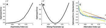
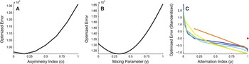
For each value of asymmetry index α, Fig. 2A plots the minimum value $O_F^{{\rm{opt}}}$ , with the minimum taken over all arrangements with that value of α. The plot confirms our statement above that for these conditions, the best performance (minimum $O_F^{{\rm{opt}}}$ ) is obtained for α = 0 (dichromatic). In addition, it shows that the worst performance is obtained for monochromatic retinas (α = 1). As the mosaic moves from equal numbers of the two classes to all of one, performance degrades in a smooth and regular fashion.

Fig. 2.

Optimized error ( $O_F^{{\rm{opt}}}$ ) for equal signal-to-noise case. This figure presents results where the mean and variance of the signals in the two wavelength bands are the same and where the two classes of photopigment have the same dark noise. (A) $O_F^{{\rm{opt}}}$ is plotted as a function of the asymmetry index, α. For each value of α, performance is plotted for the particular arrangement with that α that minimized $O_F^{{\rm{opt}}}$ . The two photoreceptor classes had γ = 0 and γ = 1, respectively, meaning that each contained a completely separate class of photopigment. Best performance is obtained for α = 0, which corresponds to equal numbers of the two photoreceptor classes. (B) $O_F^{{\rm{opt}}}$ is plotted as a function of the photopigment mixing parameter, γ, for a retina with only one class of photoreceptor. Best performance is obtained for γ = 0.5, corresponding to an equal mix of the two photopigment types. (C) Effect of regularity on performance. Each line in the plot shows $O_F^{{\rm{opt}}}$ as a function of the regularity index, ρ. Each line in the plot corresponds to a different choice of α: 0 (dark blue), ${\textstyle{1 \over 6}}$ (blue), ${\textstyle{1 \over 3}}$ (light blue), ${\textstyle{1 \over 2}}$ (light green), ${\textstyle{2 \over 3}}$ (yellow), ${\textstyle{5 \over 6}}$ (orange), and 1 (red dot). For each value of α and ρ, performance is plotted for the particular arrangement that minimized $O_F^{{\rm{opt}}}$ . In this panel, $O_F^{{\rm{opt}}}$ is plotted in standardized (z-score) units computed separately for each value of α. This allows us to compare the effect of ρ for each α without undue expansion of the scale of the y-axis. For each α, the best performance is obtained for a maximally regular arrangement (ρ = 1). As in panel A, these calculations were performed for two photoreceptor classes with γ = 0 and γ = 1, respectively. For all panels, illumination intensity (ω) was set to 2000. We set the dark noise for both photopigments to one spontaneous isomerization per unit time. We used a duration of 1 time unit for this and all other calculations in the article. The mean and variance in number of reflected quanta for both color bands were set to 1. Color correlation (r_C) was set to 0.8, and spatial correlation (r_S) was set to 0.9. The standard deviation of the Gaussian blur was set to two pixels, and the photoreceptor aperture was three pixels. All simulations were performed using 12 photoreceptors and 36 image pixels.

One might reasonably argue that the comparison above is too restrictive, as we considered only receptors with spectral sensitivity confined to one wavelength. More generally, we could consider monochromatic retinas with other spectral sensitivities. Given that our model environment has just two wavelengths, we can express spectral sensitivity through a parameter γ that describes the relative amounts of each of the two photopigments contained in a given photoreceptor. The calculations above effectively considered only γ = 0 or γ = 1, corresponding to photoreceptors containing only class 1 or class 2 photopigment. Fig. 2B shows the effect of allowing other values of γ on the performance of a monochromatic retina. The optimal value of γ is 0.5, an equal mix of the two underlying photopigments. Note, however, that the value of $O_F^{{\rm{opt}}}$ for this optimal mix (~4.5 × 10⁷) is still considerably higher than the level of performance obtained with the best dichromatic retina (~3.5 × 10⁷). Thus, even when spectral sensitivity is optimized for monochromatic vision, a dichromatic retina is better than a monochromatic retina, at least for the high illumination intensity we simulated.

Finally, note that for a given value of the asymmetry index, there may be multiple mosaics that only differ in how the two cone classes are arranged. So, for example, given that an equal number of the two receptor classes leads to best performance, we can turn to ask how these should be arranged. We defined an alternation index, ρ, that captures the extent to which the two receptors are interleaved in the overall mosaic. The computation of the alternation index begins with the computation of a raw alternation index:

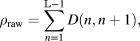
$\rho _{{\text{raw}}} = \sum\limits_{n = 1}^{{\Bbb L} - 1} {D(n,n + 1)},$

where D(u, v) = 1 if the photoreceptors at positions u and v are of different types and 0 otherwise. The value of ρ _raw is a count of the number of alternations of receptor type as one moves along the one-dimensional mosaic. Because the number of possible alternations depends on the relative number of the two receptor classes, we convert the raw alternation index to the alternation index ρ by taking the percentile ranking of ρ _raw within the set of all possible arrangements that share the same asymmetry index α and dividing by 100. This leads to an alternation index that is always in the range 0–1, that takes on a value of 0 when the two receptor classes are maximally grouped together in the mosaic and a value of 1 when the two classes alternate as much as possible.

Fig. 2C shows optimized error plotted against alternation index ρ. The plot makes it clear that arrangements that interleave the two photoreceptor classes as much as possible are preferred over less alternating arrangements. This is true for the optimal value of the asymmetry index (α = 0) as well as for other values.

Color versus monochromatic vision across illumination levels

The section above demonstrates conditions where the performance of a dichromatic retina dominates that of a monochromatic retina. The standard intuition, as discussed in the introduction, is that this situation should reverse when light level drops. To investigate, we repeated the calculations for a range of illuminant intensities ω. Note, by the way, that we are not attempting to study which factors might mediate the known shift between cone- and rod-mediated vision. To do so would require adding a model of the differences between cones and rods to our formulation and then comparing performance of each system across a range of light levels. Rather, our present goal is to compare performance of monochromatic and dichromatic mosaics within a single type of receptor. Given our focus on what happens at low light levels, this type should be conceived of as the rods.

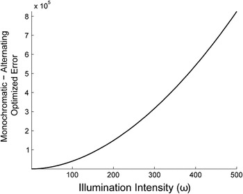
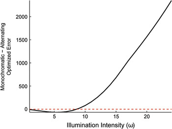
Fig. 3 plots the difference in optimized error $O_F^{{\rm{opt}}}$ between the best monochromatic retina and best dichromatic retina as a function of light level. For the monochromatic retina, we found the best value of spectral sensitivity γ for each choice of illuminant intensity ω and used this value in the comparisons. In the event, the best value was always γ = 0.5. For the dichromatic retina, we restricted attention to the case where each of the two photoreceptor classes was sensitive only to a single wavelength and used an alternating arrangement with equal numbers of photoreceptors of each class. Given the restriction to two classes, the alternating/equal number of arrangement was in fact the best for every illumination intensity. The figure shows that at every light level, the dichromatic retina outperforms the monochromatic retina.

Fig. 3.

Comparison of dichromatic and monochromatic vision for equal photoreceptor signal-to-noise and high color and spatial correlations. This figure compares the optimized error for the best dichromatic and monochromatic arrangements. The dichromatic arrangement was constrained to have γ = 0 and γ = 1 for the two photoreceptor classes and had α = 0 and ρ = 1. The monochromatic arrangement had γ = 0.5. The plot shows the difference between monochromatic and dichromatic $O_F^{{\rm{opt}}}$ as a function of illumination intensity. Positive values correspond to the case where the dichromatic arrangement has a smaller $O_F^{{\rm{opt}}}$ . For this case, dichromatic vision is better than monochromatic vision at all light levels. Signal and photoreceptor parameters were the same as in Fig. 2.

Our calculations do not confirm the standard intuition about why rod-mediated vision is almost always monochromatic. Nonetheless, it is worth noting that our calculations are consistent with some aspects of previous thinking. The core of the standard intuition is that the advantage for color vision decreases as SNR drops, and our calculations reveal this effect: the difference in $O_F^{{\rm{opt}}}$ between monochromatic and dichromatic vision tends to zero with decreasing SNR. Indeed, this is not surprising in the limit, since when signal-to-noise reaches zero, useful vision disappears and the organism’s estimates of the image are optimizing by guessing based on the mean of the image prior, independent of the receptor responses. What our results now add is the fact that a decreasing advantage of color vision does not necessarily translate into an advantage for monochromatic vision. To understand the selective advantage for monochromatic vision at night, some additional consideration must be added to the model system. We explore two possibilities below. One is the statistical characterization of the image ensemble, and the other is asymmetric signal-to-noise across the two receptor classes.

Effect of image statistics

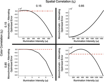
All simulations discussed above used r_S = 0.9, r_C = 0.8. Although this choice reflects a reasonable characterization of natural images, it is of interest to explore the effect of varying these parameters. Fig. 4 shows the comparison of dichromatic and monochromatic retinal designs for four choices of r_S and r_C, with other parameters the same as used to produce Fig. 3.

Fig. 4.

Comparison of color and monochromatic retinas for varying color and spatial correlations. All panels compare $O_F^{{\rm{opt}}}$ for the alternating dichromatic and best monochromatic arrangements. The dichromatic arrangement was constrained to have γ = 0 and γ = 1 for the two photoreceptor classes, with α = 0 and ρ = 1. For monochromatic arrangements, the optimal value of γ was allowed to vary with illumination intensity. The plot shows the difference between monochromatic and dichromatic $O_F^{{\rm{opt}}}$ as a function of illumination intensity. Positive values correspond to the case where the dichromatic retina is better. Spatial correlation (r_S) was set to either 0.15 (left panels) or 0.85 (right panels). Color correlation (r_C) was set to either 0.15 (top panels) or 0.85 (bottom panels). A red dashed horizontal line representing equal error for the monochromatic and dichromatic arrangements is drawn in panels containing a crossover from monochromatic to dichromatic vision being optimal. All signal and photoreceptor parameters were the same as in Fig. 2. Note that the scale of the x-axis is chosen differently in each panel, so as to better illustrate the transitions between dichromatic and monochromatic advantage.

The figure shows that dichromatic vision dominates at low light levels, regardless of spatial and color correlations. Dichromatic vision also dominates at high light levels, when r_S > r_C (panel B). However, when r_S ≤ r_C (panels A, C, and D), the high–light level pattern reverses and monochromatic vision becomes better at high light levels.

We draw two conclusions from this analysis. First, the trade-off between dichromatic and monochromatic color vision is quite sensitive to the statistical structure of the environment. This insight is consistent with consideration of limiting cases. If the color correlation r_C = 1, then there is no chromatic variation in the environment and no added benefit of a second receptor class. On the other hand, if r_S = 1, there is no spatial variation in the environment and having multiple receptor classes has clear benefits. Our calculations show that a fairly rich set of trade-offs is available across cases intermediate to these two environmental extrema.

The second conclusion we draw is that none of the r_S, r_C pairs we considered lead to a trade-off pattern consistent with the biological observations, making it likely that additional factors played an important role in the evolution of vertebrate mosaic design.

Asymmetric photopigment dark noise

All of our calculations up to this point have assumed that the two photopigment classes are equally reliable and that signals in the two color bands are equally informative. As noted in the introduction, however, for biological photoreceptors, the spontaneous isomerization rate might be expected to vary systematically with the wavelength of peak sensitivity (Platt, Reference Platt1956; Barlow, Reference Barlow1957). For this reason, we explored the effect of specifying different levels of dark noise for the two photopigments.

Fig. 5 shows, for a single intermediate illumination intensity, the effects of making one photopigment 100 times noisier than the other, by setting the dark noise ratio d ₁:d ₂ = 100. This manipulation introduces an asymmetry into the results. Unlike the symmetric case, the best dichromatic photoreceptor arrangements now contain more of the lower–dark noise photoreceptors (Fig. 5A). Similarly, the best monochromatic arrangements contain more of the lower–dark noise photopigment (Fig. 5B). As for the symmetric case, however, Fig. 5C shows that maximizing the alternation index (ρ = 1) optimizes performance.

Fig. 5.

Optimized error ( $O_F^{{\rm{opt}}}$ ) for unequal dark noise case. This figure presents results where the mean and variance of the signals in the two wavelength bands are the same but where the dark noise of class 1 photopigment is 100 times greater than that of class 2 photopigment. (A) $O_F^{{\rm{opt}}}$ is plotted as a function of the asymmetry index, α. The two photoreceptors had γ = 0 and γ = 1, respectively. Best performance is obtained for $\alpha = {\textstyle{1 \over 6}}$ , which corresponds to an arrangement containing five class 1 photoreceptors for every seven class 2 photoreceptors. (B) $O_F^{{\rm{opt}}}$ is plotted as a function of the photopigment mixing parameter, γ, for a retina with only one class of photoreceptor. Best performance is obtained for γ = 0.32, which corresponds to a mix of 32% class 1 photopigment and 68% class 2 photopigment. (C) Effect of regularity on performance. Each line in the plot corresponds to a different choice of α: 0 (dark blue), ${\textstyle{1 \over 6}}$ (blue), ${\textstyle{1 \over 3}}$ (light blue), ${\textstyle{1 \over 2}}$ (light green), ${\textstyle{2 \over 3}}$ (yellow), ${\textstyle{5 \over 6}}$ (orange), and 1 (red dot). For each value of α and ρ, performance is plotted in standardized (z-score) units computed separately for each value of α. For all values of α, best performance is obtained for a maximally regular arrangement (ρ = 1). As in panel A, these calculations were performed for two photoreceptor classes with γ = 0 and γ = 1, respectively. For all panels, illumination intensity (ω) was set to 75. The mean and variance in number of reflected quanta for both color bands were set to 1. Color correlation (r_C) was set to 0.8, and spatial correlation (r_S) was set to 0.9. The standard deviation of the Gaussian blur was set to two pixels, and the photoreceptor aperture was three pixels. All simulations were performed using 12 photoreceptors and 36 image pixels.

The most striking new result to emerge from the asymmetric dark noise calculations is shown in Fig. 6. Recall that dichromatic arrangements always outperformed monochromatic arrangements for the symmetric case, regardless of SNR (Fig. 3). With the inclusion of asymmetric dark noise, dichromatic arrangements still outperform monochromatic arrangements at high illumination intensities. As illumination intensity decreases and SNR drops, however, monochromatic arrangements lead to lower optimized error. This effect can be explained by the following intuition. At high light levels, photon noise dominates dark noise and the asymmetry between photopigment dark noise has a negligible effect. In this case, the extra information about the image transduced by a dichromatic retina is the dominant factor. At low light levels, dark noise becomes the dominant noise source, and the noise advantage of the less noisy photopigment drives the optimal design.

Fig. 6.

Comparison of dichromatic and monochromatic vision for unequal photopigment dark noise and high color and spatial correlations. We compare $O_F^{{\rm{opt}}}$ for the alternating dichromatic and best monochromatic arrangements. The dichromatic arrangement was constrained to have γ = 0 and γ = 1 for the two photoreceptor classes and had α = 0 and ρ = 1. The optimal value of γ for the monochromatic arrangement was allowed to vary with illumination intensity. The plot shows the difference between monochromatic and dichromatic $O_F^{{\rm{opt}}}$ as a function of illumination intensity. Positive values correspond to the case where the dichromatic arrangement has a smaller $O_F^{{\rm{opt}}}$ . For this case, monochromatic vision is better at low light levels, and color vision is better at high light levels. Signal and photoreceptor parameters were the same as in Fig. 5.

The crossover illumination intensity, below which monochromatic vision dominates and above which dichromatic vision dominates, depends on the relative reliability of the two photopigments. As one photoreceptor class becomes more unreliable relative to the other, the illumination intensity at which color vision becomes beneficial increases (not shown).

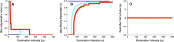
In Fig. 7, we systematically explore how the optimal dichromatic and monochromatic photoreceptor arrangements change with illumination intensity. In each panel, the three colored lines correspond to three d ₁:d ₂ ratios. For reference, the case where d ₁ = d ₂ is shown in dark blue. For this case, independent of illumination intensity, the best dichromatic arrangements have equal numbers of the two photoreceptor classes, arranged in an alternating pattern (α = 0, ρ = 1), while the best monochromatic arrangements have equal amounts of the two photopigments (γ = 0.5). As d ₁:d ₂ is increased, optimal arrangements exhibit asymmetries in the relative numbers of photoreceptors (or amounts of photopigment) at lower illumination intensities. The figure shows that the rate at which the arrangements return to having equal number of photoreceptors of each class (or equal amounts of the two photopigments) as a function of illumination intensity depends on the d ₁:d ₂ ratio. The shifts in optimal spectral sensitivity with light level for monochromatic mosaics (panel B) are an analog, within our model system, of the Purkinje shift as analyzed by Barlow (Reference Barlow1957). For all conditions studied, it is always best to interleave photoreceptors as much as possible (panel C, ρ = 1).

Fig. 7.

Best (A) asymmetry index, (B) mixing parameter, and (C) alternation index, as a function of illumination intensity (ω). For all panels, class 1 photopigment is as reliable as class 2 photopigment (blue), 400× more reliable than class 2 photopigment (cyan), or 1000× more reliable than class 2 photopigment (red). Class 1 photopigment had a dark noise of one spontaneous isomerization per unit time. Signal and photoreceptor parameters were the same as in Fig. 2. Note that in panel C, all three curves lie on top of each other.

Introducing an asymmetry in the level of dark noise for different photopigments is not the only way to produce an asymmetry in the SNR of the output of different photoreceptor classes. Such asymmetries can also be produced if the mean light level is different across wavelengths; if there is a difference in the degree of retinal absorption across wavelengths (as might be produced by protective ultraviolet-absorbing macular pigment); if there is a difference in the quantal efficiency of different photopigments; or if the variance in the signals at different wavelengths differs. We would expect that effects similar to those shown above for the asymmetric dark noise case would also be produced by signal asymmetries. Indeed, we explored this explicitly for the case of unequal signal variance and found a pattern of results similar to that shown in Figs. 5 and 6. In the interest of brevity, we do not present those results here.

Optimizing dichromatic spectral sensitivity

In the calculations above for dichromatic mosaics, we considered only photoreceptor classes with γ = 0 and γ = 1, respectively. Across species, there is variation in the degree of overlap between photoreceptor spectral sensitivities between photoreceptors of different classes. For example, in goldfish the peak sensitivities of the M and L cones are noticeably more separated, at 530 and 620 nm, respectively, than in primates, where the peak sensitivities are approximately 530 and 560 nm, respectively (Bowmaker, Reference Bowmaker, Cronly-Dillon and Gregory1991). We wondered what the optimal choices of spectral sensitivity were in our model system.

To study this while avoiding parameter explosion, we considered how $O_F^{{\rm{opt}}}$ varied with a parameter η, where the photoreceptor sensitivities of the two classes depend on η through γ ₁ = η and γ ₂ = 1 − η. We studied mosaics with equal numbers of receptors from each class in an alternating arrangement. Note that when η = 0.5, the dichromatic arrangement is equivalent to the monochromatic arrangement with γ = 0.5, while η = 0 and η = 1 reduce to the dichromatic arrangements studied above.

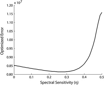
Fig. 8 plots $O_F^{{\rm{opt}}}$ as a function of η, for the alternating dichromatic arrangement, at a single illumination intensity. The computed function has two minima, at the symmetric locations η = 0.27 and η = 0.73.Footnote ⁴ Adding some degree of spectral overlap between the two photoreceptor classes improves performance, but too much overlap has a significant deleterious effect. Indeed, in the limit of η = 0.5, this is simply a reexpression of the fact that monochromatic retina does worse than a dichromatic retina.

Fig. 8.

Effect of spectral sensitivity. This figure plots $O_F^{{\rm{opt}}}$ as a function of the spectral sensitivity parameter η, for the alternating arrangement (α = 0, ρ = 1), at a single illumination intensity (ω = 1000). The optimal values of η are 0.27 and 0.73, corresponding to mixes of 27% of one photopigment and 73% of the other. Aside from illumination intensity and photopigment mixing parameters, the signal and photoreceptor parameters were the same as in Fig. 2. Since this figure is symmetric about η = 0.5, we restrict the domain displayed to 0 ≤ η ≤ 0.5.

Fig. 8 shows results for the case of symmetric receptor dark noise. In the asymmetric case, the same value of η characterizes optimal design for high light levels (since at high light levels, dark noise is dominated by photon noise). Because our results in Fig. 6 were obtained for η = 0 (or equivalently η = 1), it is possible that the advantage for monochromatic vision at low light levels shown in the figure would reverse if the calculations were performed with optimized dichromatic spectral sensitivity. We ruled out this possibility by verifying that monochromatic vision continues to dominate at low light levels in the asymmetric dark noise case, even for η = 0.27 (or equivalently η = 0.73).

More generally, one could consider whether any dichromatic retina outperforms a monochromatic retina at low light levels, for the asymmetric dark noise case. Exploring all possible choices of spectral sensitivity for the two receptor classes for all possible arrangements is computationally prohibitive. But since a monochromatic retina represents a limiting case of a dichromatic retina where the spectral sensitivities of the two classes become progressively more similar, and where the asymmetry index approaches unity, we can ask whether making a monochromatic retina a just little bit dichromatic improves performance or worsens it. To do so, we compared the performance of a monochromatic retina with all receptors containing the low–dark noise photopigment to that of a retina where a small amount (10%) of the high–dark noise photopigment had been added to a single photoreceptor in the array. We found that for the asymmetric dark noise case, the purely monochromatic retina led to superior performance at low illumination levels. This in turn suggests that, indeed, the purely monochromatic retina represents a global optimum in design.

Discussion

Animals have evolved sense organs that are near-optimal for detecting and measuring changes in the environment. For example, rod photoreceptors can reliably transduce the energy of a single quantum of light (Baylor et al., Reference Baylor, Lamb and Yau1979); hair cells in the ear are sensitive to deflections as small as the radius of a single hydrogen atom (Sellick et al., Reference Sellick, Patuzzi and Johnstone1982); and olfactory sensory neurons can respond to the arrival of a single molecule of odorant (Schneider, Reference Schneider1969).

More generally, many properties of sensory systems have been successfully understood as near-optimal solutions to information uptake and processing problems. For example, the design of a fly’s compound eye has been shown to represent an optimal trade-off between spatial resolution and sensitivity to contrast (Snyder et al., Reference Snyder, Stavenga and Laughlin1977); the spectral properties of primate cone photoreceptors optimize discrimination of fruit from foliage (Regan et al., Reference Regan, Julliot, Simmen, Vienot, Charles-Dominique and Mollon2001); properties of retinal ganglion cells optimize information transmission down the optic nerve (Buchsbaum & Gottschalk, Reference Buchsbaum and Gottschalk1983; Atick, Reference Atick1992; Atick et al., Reference Atick, Li and Redlich1992; van Hateren, Reference van Hateren1992, Reference van Hateren1993; von der Twer & MacLeod, Reference von der Twer and MacLeod2001; Koch et al., Reference Koch, McLean, Berry, Sterling, Balasubramanian and Freed2004); and adaptation maximizes the use of limited neural dynamic range across changes in environmental conditions (Laughlin & Hardie, Reference Laughlin and Hardie1978; Walraven et al., Reference Walraven, Enroth-Cugell, Hood, MacLeod, Schnapf, Spillman and Werner1990).

Optimality calculations provide a principled null model against which to benchmark the performance of sensory and other information processing systems (Geisler, Reference Geisler1987; Watson, Reference Watson1987; Brainard, Reference Brainard and Masin1993). In addition, showing how a feature of a biological system is closely matched to predictions derived from considerations of optimality provides a satisfying, if speculative, answer to the question of why that particular feature evolved.

In this article, we develop a theoretical methodology to evaluate the quality of different choices of retinal photoreceptor mosaic. Our method is based on Bayesian decision theory (Blackwell & Girschick, Reference Blackwell and Girschick1954; Berger, Reference Berger1985; Gelman et al., Reference Gelman, Carlin, Stern and Rubin2004). Similar underlying logic was employed by Srinivasan et al. (Reference Srinivasan, Laughlin and Dubs1982) in the context of understanding the receptive fields of retinal ganglion cells, and our general formulation closely parallels that developed independently by Levin et al. (Reference Levin, Durand and Freeman2008) to evaluate the design of digital cameras.

We applied our method in the context of a simplified model system to investigate three fundamental questions about retinal design. First, we showed that for dichromatic retinas, regular arrangements that maximally alternate between the two types of photoreceptors lead to better performance than less regular arrangements. Second, introducing overlap between the spectral sensitivities of the photoreceptors of dichromatic retinas can improve performance. Third, when we compare dichromatic and monochromatic retinas, we find that which is optimal is quite sensitive to the specific parameters chosen within our model system. In the symmetric case where the different photoreceptor types have the same level of intrinsic noise and the different wavelengths carry the same amount of signal, a dichromatic retina yields best performance at all SNRs, when the correlations between neighboring image locations are higher than those between neighboring wavelength bands. To obtain results that mirror what is typically found in biological systems (monochromatic vision for low–signal-to-noise conditions and color vision for high–signal-to-noise conditions), we had to introduce an asymmetry between the SNRs of the two photoreceptor classes.

Measurements of photoreceptor dark noise

A number of laboratories have measured photoreceptor dark noise for receptors with different pigment spectral sensitivities. For our analysis here, the most relevant measurements are those for rods, which mediate vertebrate vision at low light levels. Baylor et al. (Reference Baylor, Nunn and Schnapf1984) showed that thermal-like events dominate the dark noise of primate rods, suggesting strongly that at the lowest light levels, it is thermal noise rather than later noise that sets the limit on performance. Ala-Laurila et al. (Reference Ala-Laurila, Pahlberg, Koskelainen and Donner2004) measured the activation energy for 12 visual pigments varying in λ _max and found that activation energy decreased with λ _max, although the decrease was shallower than the 1/λ _max dependence that would be predicted if the only factor involved was the energy of photons at wavelength of peak sensitivity. This result does not directly show that receptor dark noise depends on λ _max but does confirm a key feature of the theory that predicts such dependence. More recently, Ala-Laurila et al. (Reference Ala-Laurila, Donner, Crouch and Cornwall2007) estimated thermal noise rates for two forms of rhodopsin in isolated salamander rods and concluded that the noise was larger for the form with longer λ _max. Taken together, these two results make it highly plausible that there are fundamental dark noise asymmetries across rod photoreceptors with different wavelengths of peak sensitivity, as Barlow (Reference Barlow1957) hypothesized.

Rieke and Baylor (Reference Rieke and Baylor2000) compared dark noise in salamander S and L cones and found that the noise in L cones was much greater. For L cones, they concluded that dark noise was dominated by thermal isomerizations. For S cones, other noise sources dominated. Their results are consistent with a dependence of dark noise on 1/λ _max. On the other hand, Schneeweis and Schnapf (Reference Schneeweis and Schnapf1999) found little difference in the dark noise levels of primate M and L cones, perhaps because the dark noise in these receptors is dominated by sources other than thermal isomerizations. It is probably wise to keep in mind that across receptor types and species, the relationship between λ _max and dark noise may not be simple. For our present purposes, however, the crucial point is that at the lowest light levels, asymmetries in rod thermal noise across receptor types seem likely to play an important role in retinal design.

Relation to other work: Color vision at night

As noted in the introduction, other authors have considered why monochromatic vision pervades at low light levels. Although our calculations here do not contradict the core observation of what we have called the standard intuition on this matter (van Hateren, Reference van Hateren1993; Land & Osorio, Reference Land and Osorio2003), they show that the standard intuition alone is insufficient and requires more careful elaboration. Indeed, in the absence of any asymmetry in the noise properties of photoreceptor types or in the signal carried by different image wavelengths, a dichromatic retina can outperform a monochromatic retina at all SNRs. This conclusion holds for the case where the spatial correlation between neighboring image locations is higher than the color correlation across neighboring image wavelengths.

We are, however, able to show that monochromatic vision dominates dichromatic vision at low light levels if we introduce an asymmetry across photoreceptor types or between the statistics at different image wavelengths. Such asymmetries then interact with SNR to drive a shift in optimal mosaic arrangement. The critical role of the noise asymmetry parallels Barlow’s (Reference Barlow1957) explanation of the Purkinje shift. As discussed in the previous section, there is good reason to believe that there are in fact asymmetries in rod noisiness with changes in photopigment λ _max. Less is known about possible asymmetries in the signals carried at different image wavelengths, but these may also exist. Thus, our analysis provides a plausible explanation for the rarity of color vision at night but only with the assumption of asymmetries.

Note that our work does not contradict van Hateren’s (Reference van Hateren1993) results, as there are several key differences between his analysis and ours. First, we explicitly compare the performance of interleaved dichromatic retinas with that of monochromatic retinas. This is quite different than asking, for any particular retina, whether the optimal processing of the output of that retina tends toward luminance processing at low light level. Second, considering the properties of the optimal single channel, as van Hateren did, is different from asking whether adding a second channel might improve performance.

Finally, we note that we can replicate van Hateren’s (Reference van Hateren1993) basic conclusion within the context of our current model. We asked, for the case where the two receptor classes have equal SNR, how the reconstruction of luminance (both receptor types stimulated together) and chromatic (the two receptor types stimulated in opposition) signals compared as a function of SNR (results not shown). We found, consistent with van Hateren, that the magnitude of the reconstructed chromatic signal decreased relative to that of the reconstructed luminance signal as overall SNR dropped. This calculation is consistent with the standard intuition. Interestingly, it is also consistent with the observed achromatic interval found for cone-mediated foveal viewing in humans: as light level drops, there is a regime where dim test lights can be detected but not be judged in color (Walraven, Reference Walraven1962; Graham & Hsia, Reference Graham and Hsia1969). Massof (Reference Massof1977) presents a model where detection is limited by quantum fluctuations that account for this interval.

Relation to other work: Mosaic regularity

In all our calculations, we found that the best arrangement of the multiple (in this case two) receptor classes is regular, in the sense that it maximizes the number of alternations between classes across the mosaic. This result is consistent with the regular mosaic layout found in fish (Scholes, Reference Scholes1975; Bowmaker & Kunz, Reference Bowmaker and Kunz1987) and with the regular arrangement of the S cone submosaic in humans (Curcio et al., Reference Curcio, Allen, Sloan, Lerea, Klock and Milam1991) but not with the quasi-random arrangement of L and M cone submosaics in primates (Mollon & Bowmaker, Reference Mollon and Bowmaker1992; Hofer et al., Reference Hofer, Carroll, Neitz, Neitz and Williams2005).

A few investigators have considered the effect of photoreceptor irregularity on performance. Most of this work is in the context of the spatial arrangement of monochromatic mosaics rather than the arrangement of interleaved submosaics. The principles considered in the earlier work, however, are of a general nature and might reasonably be taken to apply to the current case.

Bossomaier et al. (Reference Bossomaier, Snyder and Hughes1985) concluded that mosaic irregularity had a deleterious effect on performance, consistent with our general conclusion. Their analysis, however, was based on the assumption that the visual system processed the output of the irregular mosaic as if the receptors were in fact regularly spaced. In this case, the effect of irregular spacing may be mimicked by the addition of noise to the output of a regular mosaic, and the addition of such noise would degrade performance. Recent modeling of the appearance of very small flashed spots (Brainard et al., Reference Brainard, Williams and Hofer2008), however, indicates that the human visual system does take the fine spatial structure of its mosaic into account. In any case, the key difference between the development of Bossomaier et al. (Reference Bossomaier, Snyder and Hughes1985) and the one presented here is that their conclusion hinges on the assumption that the visual system’s postreceptoral processing is suboptimal, while ours evaluates each mosaic arrangement on the assumption that postreceptoral processing optimally accounts for the location of each photoreceptor.

Yellott (Reference Yellott1982, Reference Yellott1983) concluded, on the other hand, that mosaic irregularity can improve visual performance. He analyzed the nature of the set of spatial aliases for different mosaic arrangements. (Two different images are aliases for a mosaic if they produce the same response in every photoreceptor in the mosaic.) For regularly arranged mosaics, regular spatial patterns at high spatial frequencies (e.g., high–spatial frequency sinusoids) have as aliases other regular spatial patterns at lower spatial frequencies (e.g., low–spatial frequency sinusoids). For irregularly arranged mosaics, regular high–spatial frequency patterns alias in to irregular low–spatial frequency patterns that appear as spatial noise. Yellott pointed out that a visual system that incorporated knowledge of the spatial structure in natural scenes would be better able to filter the low–spatial frequency aliases produced by an irregular mosaic than the those produced by a regular mosaic, suggesting a possible advantage for irregular mosaics.

Yellott’s argument could be formalized and evaluated within the framework presented here. The key extension to current analysis required for this would be to choose an image prior that incorporates a preference for structured images; the Gaussian priors we used capture only the second-order structure of natural images and do not allow expression of higher order structure that favors, for example, the presence of edges. Whether such an analysis would lead to a rationale for irregular mosaics within our simple model system remains an open question of considerable interest.

Finally, Hsu et al. (Reference Hsu, Smith, Buchsbaum and Sterling2000) argued that in the presence of electrical coupling between receptors of different classes, irregularity in the interleaving of these classes would reduce the deleterious effects of the coupling on color vision. DeVries et al. (Reference DeVries, Qi, Smith, Makous and Sterling2002) complemented this line of thinking by observing that the same coupling could reduce noise at the receptor outputs by integrating over multiple receptors and that the cost of such coupling for spatial vision was not significant in the presence of optical blur. We have not explored these results in the context of our model system. Doing so would require imposing specific processing steps after the receptors (e.g., modeling electrical coupling) and then asking how the added processing constraint affected retinal design.

Relation to other work: Spectral sensitivity

A number of authors have considered the interaction of spectral properties of the photic environment and cone spectral sensitivity. The theoretical approach taken by Lewis and Zhaoping (Reference Lewis and Zhaoping2006) is quite similar to ours, although their performance criterion is one of maximizing information rather than minimizing Bayes’ risk (see below). These authors conclude that the λ _max of the human L cone is not optimally located, as more information would be transmitted if its peak sensitivity were at a higher wavelength. As with our work, a key factor that drives their calculations is asymmetry between the information available for photoreceptors with different wavelengths of peak sensitivity. In particular, they note that as overall SNR decreases, the optimal placement of both L and M cones tends toward the wavelength that provides maximum signal-to-noise. This is analogous to our conclusion that the optimal mosaic tends toward monochromatic as signal-to-noise decreases. One important difference between our work and theirs is that we explicitly evaluate spatial and spectral performance jointly, whereas they do not treat spatial variation.

Other articles in this general tradition (Lythgoe & Partridge, Reference Lythgoe and Partridge1989; Chittka & Menzel, Reference Chittka and Menzel1992; Osorio & Vorobyev, Reference Osorio and Vorobyev1996; Regan et al., Reference Regan, Julliot, Simmen, Vienot, Charles-Dominique and Mollon2001; Cummings, Reference Cummings2004) analyze performance on a particular color discrimination task thought to be important for the organism (e.g., discriminating fruits from foliage for primates; Regan et al., Reference Regan, Julliot, Simmen, Vienot, Charles-Dominique and Mollon2001) as a function of choice of spectral sensitivity. This work shares with our current analysis emphasis both on the statistical properties of stimuli that will be encountered by the visual system and on optimizing performance. The specifics of the analyses differ, with our work considering a highly simplified visual environment. This allows us to explore a wider range of parametric interactions, at the cost of departing further from ecologically valid measurements.

Relation to other work: Theory

Our approach to optimal design employs formalism taken from Bayesian decision theory. An alternative and closely related approach is to consider not minimization of expected loss but rather maximization of transmitted information, as measured in bits. Analyses based on information theory have been successfully employed to explain features of postreceptoral retinal design (e.g., Atick, Reference Atick1992; Brenner et al., Reference Brenner, Bialek and de Ruyter van Steveninck2000; Balasubramanian & Berry, Reference Balasubramanian and Berry2002; Koch et al., Reference Koch, McLean, Berry, Sterling, Balasubramanian and Freed2004). In the current context, the difference between the two approaches is straightforward to understand. Given a fixed prior distribution over images, the design that maximizes information transmission is the one that leads to a posterior distribution with minimum entropy (Cover & Thomas, Reference Cover and Thomas1991). Entropy is a measure of the uncertainty in the outcome of draws from a distribution. A posterior distribution with low uncertainty, generally speaking, is also one that will lead to low estimation error with respect to a specified loss function. However, the relation between entropy and expected loss need not be monotonic (Thomson & Kristan, Reference Thomson and Kristan2005).

Given that minimizing expected loss and maximizing information transmitted do not always lead to the same conclusion, one could reasonably ask which approach is more appropriate. The attraction of minimizing expected loss is that it allows explicit inclusion of what matters to the organism, and it is for this reason that we have used the Bayesian approach here. At the same time, we concede that the specific choice of squared error loss is at best a crude approximation to what matters to most organisms and in the current work serves as a placeholder where more realistic loss functions can be inserted when such are available. This general point, that information theory tends to be insensitive to the metric structure of the stimulus space, is discussed by Luce (Reference Luce2003). We did verify that the main features of the results reported in this article (i.e., the monochromatic–dichromatic comparisons shown in Figs. 3 and 6) continue to hold when the calculations are repeated with maximizing transmitted information as a criterion. The one exception we found is that increasing the overlap in spectral sensitivity, which improves performance for a dichromatic retina as assessed by minimizing expected squared error loss (Fig. 8), does not increase information transmitted.

An advantage of information theory that drives its use in many studies of neural systems is that there are techniques for measuring the information carried by a neuron that do not require knowledge of the analytic form of the stimulus ensemble or of the representation coded by the neural response. Thus, for example, the information about natural images conveyed by a particular ganglion cell may be estimated by measuring the cells’ response to a sequence of presented natural images, without need to develop an explicit algorithm for estimating images from the response (e.g., Brenner et al., Reference Brenner, Bialek and de Ruyter van Steveninck2000; Balasubramanian & Berry, Reference Balasubramanian and Berry2002; Koch et al., Reference Koch, McLean, Berry, Sterling, Balasubramanian and Freed2004). In this sense, information theory is an approach that complements the one we have taken here. Indeed, in related work, we are considering features of mosaic design using information theoretic methods (Garrigan et al., Reference Garrigan, Ratliff, Klein, Sterling, Brainnard and Balasubramanian2006, Reference Garrigan, Ratliff, Klein, Sterling, Brainard and Balasubramanian2008).

Future directions

The model system explored in this article was very simple. Nonetheless, it allowed us to express many of the pieces required for a full theory of optimal mosaic design. These are a specification of the statistical properties of the visual environment, specification of the relation between an image and its sensory representation, and specification of the goal of the visual computation as a loss function. Given these, we could explore the performance of different design choices. Despite the fact that that the model system we used is simple, we were able to demonstrate a number of conclusions. The first is that classic arguments for why monochromatic vision is favored over color vision at low signal-to-noise levels are incomplete. That is, we were able to demonstrate conditions where color vision provides better performance as signal-to-noise drops to zero. Moreover, our analysis suggested additional factors that when incorporated into the analysis do yield a shift from color to monochromatic vision as SNR drops. Second, within the context of our model system, regular mosaics dominate irregular mosaics. We have not yet found factors that would predict a robust advantage for the quasi-random tiling of L and M cones found in primate retina. Here our analysis clarifies not what we understand but what we have yet to make sense of.

Because our model system is simple, an important goal for future work is to generalize the analysis and bring it closer to biological realism. Obvious generalizations include adding a second spatial dimension, additional wavelengths (i.e., full spectra), time and motion, and additional receptor classes. There is no conceptual obstacle to these generalizations, but given present computing resources, it is not possible to explore these added dimensions exhaustively, as we could for the simple case. The challenge is to pick specific manipulations of interest. Moving in this direction would also allow incorporation of additional factors such as whether the statistics of spectra shift systematically between day and night, something we have not yet considered. These generalizations would also enable us to draw the numerical values used for spectral sensitivity and dark noise more directly from biological measurements; the present calculations are sufficiently abstracted from real retinas that we thought such an effort premature.

Computations cost energy, and energy considerations are nontrivial for the design of biological systems (Balasubramanian et al., Reference Balasubramanian, Kimber and Berry2001; Laughlin, Reference Laughlin2001; Balasubramanian & Berry, Reference Balasubramanian and Berry2002; Laughlin & Sejnowski, Reference Laughlin and Sejnowski2003). The general framework we have presented could be extended to include considerations of energetic cost. If we think of the loss function as expressing the cost of misestimation in terms of its ultimate effect on reproductive success, we can also conceive of a function that expresses the cost of computing an estimate from the receptor responses. Denote by the energetic cost function $C_F (\vec r)$ the energetic cost incurred when the estimator F() acts on input $\vec r$ . In analogy to the Bayes’ risk, we can then associate an expected computational cost with the estimator:

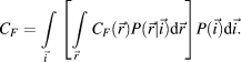
$C_F = \int\limits_{\vec i} {\left[ {\int\limits_{\vec r} {C_F (\vec r)P(\vec r|\vec i){\rm{d}}\vec r} } \right]P(\vec i){\rm{d}}\vec i} .$

Once computational cost is specified, a more general optimality principle would be to choose an estimator F() that minimizes O_F = R_F + C_F.Footnote ⁵ Note that this formulation for computational cost would also allow for consequences of the time taken to do the computation (Koch et al., Reference Koch, McLean, Segev, Freed, Berry, Balasubramanian and Sterling2006) and for variations in cost that arise from variation in the size and mass of the computational apparatus (Laughlin & Sejnowski, Reference Laughlin and Sejnowski2003). It might be reasonable to make initial steps toward including energetic cost by examining the number of multiplications and additions required to closely approximate the optimal estimator for each mosaic.

As noted in the Results section, we have not explicitly modeled differences between rods and cones, such as differences in the source and level of receptor dark noise (see above), or between properties of receptors across species. Because our formulation is very general, such differences could be included. Modeling the properties of rods and cones would, for example, allow us to address questions such as at what light level a visual system that has both rods and cones should switch from one to the other. Similarly, comparing the details of rod properties and other retinal design factors across species might provide insight as to why some species do exhibit rod-mediated color vision (Land & Osorio, Reference Land and Osorio2003; Kelber & Roth, Reference Kelber and Roth2006).

Even within our simple one-dimensional, two-wavelength system, we did not explore all possible parametric manipulations. For example, one could explore trade-offs between optical blur and pupil aperture or effects of overall receptor density. One could also try to refine the statistical model of image structure by incorporating a characterization of the edge-like features that are pervasive in natural images (Simonceli, Reference Simonceli and Bovik2005) or the model of the likelihood function (e.g., by incorporating a Poisson rather than Gaussian noise model; L. Paninski, personal communication). Finally, it would be of interest to explore effects of varying the loss function, for example, to emphasize either luminance or chromatic estimation error. This would be a first step to modeling species differences in what stimuli are most ecologically relevant. More generally, examining properties of the estimator itself could yield insights about how postreceptoral processing should be configured to optimally extract information from interleaved receptor mosaics.

Acknowledgments

We thank V. Balasubramanian, J. Bowmaker, P. Garrigan, C. Ratliff, F. Rieke, and two anonymous reviewers for useful comments on this work or pointers to relevant literature. Supported by NEI RO1 EY10016 and NIH RO1 MH61975.

Footnotes

¹ This statement holds as long as the responses of the two receptor classes are positively correlated.

² The literature generally shows not correlations across wavelength but rather correlations across responses of different classes of cones. The reported correlations across cone classes arise both because of correlations across wavelength and because of the broadband spectral sensitivity of the cones. We have verified, using the data of Ruderman et al. (Reference Ruderman, Cronin and Chiao1998), that the correlations across wavelength are in fact strong. For two narrowband images separated by 50 nm, the average correlation is about 0.9. The correlation remains above 0.8 for wavelength separations of 200 nm.

³ In using and interpreting this and our other index expressions, we only consider the case where ${\Bbb L}$ is even, a condition that holds for all results reported in this article.

⁴ The symmetry arises because for the case studied, there is no effect of reversing the labels given to the two photoreceptor classes. For this reason, only half of the computed function is shown in the plot.

⁵ The use of a simple sum is appropriate on the assumption that the measures of loss and energetic cost can be expressed in the same units. This seems reasonable in principle but may be difficult to achieve in practice.

References

Aguilar, M. & Stiles, W.S. (1954). Saturation of the rod mechanism of the retina at high light levels. Journal of Modern Optics 1, 59–65.Google Scholar

Ala-Laurila, P., Donner, K., Crouch, R.K. & Cornwall, M.C. (2007). Chromophore switch from 11-cis-dehydroretinal (A2) to 11-cis-retinal (A1) decreases dark noise in salamander red rods. Journal of Physiology 585, 57–74.CrossRef Google Scholar PubMed

Ala-Laurila, P., Pahlberg, J., Koskelainen, A. & Donner, K. (2004). On the relation between the photoactivation energy and the absorbance spectrum of visual pigments. Vision Research 44, 2153–2158.CrossRef Google Scholar PubMed

Atick, J.J. (1992). Could information theory provide an ecological theory of sensory processing. Network: Computation in Neural Systems 3, 213–251.CrossRef Google Scholar

Atick, J.J., Li, Z.P. & Redlich, A.N. (1992). Understanding retinal color coding from first principles. Neural Computation 4, 559–572.CrossRef Google Scholar

Balasubramanian, V. & Berry, M.J. (2002). A test of metabolically efficient coding in the retina. Network, 13, 531–552.CrossRef Google Scholar PubMed

Balasubramanian, V., Kimber, D. & Berry, M.J. (2001). Metabolically efficient information processing. Neural Computation 13, 799–815.CrossRef Google Scholar PubMed

Barlow, H.B. (1956). Retinal noise and absolute threshold. Journal of the Optical Society of America 46, 634–639.CrossRef Google Scholar PubMed

Barlow, H.B. (1957). Purkinje shift and retinal noise. Nature 179, 255–256.CrossRef Google Scholar PubMed

Baylor, D.A., Lamb, T.D. & Yau, K.W. (1979). Responses of retinal rods to single photons. Journal of Physiology (London) 288, 613–634.CrossRef Google Scholar PubMed

Baylor, D.A., Nunn, B.J. & Schnapf, J.L. (1984). The photocurrent, noise, and spectral sensitivity of rods of the monkey macaca fascicularis. Journal of Physiology (London) 357, 575–607.CrossRef Google Scholar PubMed

Berger, T.O. (1985). Statistical Decision Theory and Bayesian Analysis. New York: Springer-Verlag.CrossRef Google Scholar

Blackwell, D. & Girschick, M.A. (1954). Theory of Games and Statistical Decisions. New York: Wiley.Google Scholar

Bossomaier, T.R.J., Snyder, A.W. & Hughes, A. (1985). Irregularity and aliasing: Solution? Vision Research 25, 145–147.CrossRef Google Scholar PubMed

Bowmaker, J.K. (1991). The evolution of vertebrate visual pigments and photoreceptors. In Vision and Visual disfunction, vol.2, ed. Cronly-Dillon, J.R. & Gregory, R.L., pp. 63–81. London: Macmillan.Google Scholar

Bowmaker, J.K. & Kunz, Y.W. (1987). Ultraviolet receptors, tetrachromatic colour vision and retinal mosaics in the brown trout (salmo trutta): Age-dependent changes. Vision Research 27, 2101–2108.CrossRef Google Scholar PubMed

Brainard, D.H. (1993). Perceptual variability as a fundamental axiom of perceptual science: Comments on Ashby and Lee. In Foundations of Perceptual Theory, ed. Masin, S.C., pp. 385–388. Amsterdam: Elsevier Science Publishers.Google Scholar

Brainard, D.H., Williams, D.R. & Hofer, H. (2008). Trichromatic reconstruction from the interleaved cone mosaic: Bayesian model and the color appearance of small spots. Journal of Vision 8, 15, 1–23.CrossRef Google Scholar PubMed

Brenner, N., Bialek, W. & de Ruyter van Steveninck, R. (2000). Adaptive rescaling maximizes information transmission. Neuron 26, 695–702.CrossRef Google Scholar PubMed

Buchsbaum, G. & Gottschalk, A. (1983). Trichromacy, opponent colour coding and optimum colour information transmission in the retina. Proceedings of the Royal Society of London B 220, 89–113.Google Scholar PubMed

Burns, M. & Arshavsky, V. (2005). Beyond counting photons: Trials and trends in vertebrate visual transduction. Neuron 48, 387–401.CrossRef Google Scholar PubMed

Burton, G.J. & Moorehead, I.R. (1987). Color and spatial structure in natural images. Applied Optics 26, 157–170.CrossRef Google Scholar

Chittka, L. & Menzel, R. (1992). The evolutionary adaptation of flower colours and the insect pollinators’ colour vision. Journal of Comparative Physiology A: Neuroethology, Sensory, Neural, and Behavioral Physiology 171, 171–181.CrossRef Google Scholar

Cover, T.M. & Thomas, J.A. (1991). Elements of Information Theory. New York: John Wiley & Sons.Google Scholar

Cummings, M.E. (2004). Modelling divergence in luminance and chromatic detection performance across measured divergence in surfperch (embiotocidae) habitats. Vision Research 44, 1127–1145.CrossRef Google Scholar PubMed

Curcio, C.A., Allen, K., Sloan, K., Lerea, C., Klock, I. & Milam, A. (1991). Distribution and morphology of human cone photoreceptors stained with anti-blue opsin. Journal of Comparative Neurology, 312, 610–624.CrossRef Google Scholar PubMed

Demontis, G.C., Bisti, S. & Cervetto, L. (1993). Light sensitivity, adaptation and saturation in mammalian rods. Progress in Brain Research 95, 15–24.CrossRef Google Scholar PubMed

DeVries, S., Qi, X., Smith, R.G., Makous, W. & Sterling, P. (2002). Electrical coupling between mammalian cones. Current Biology 12, 1900–1907.CrossRef Google Scholar PubMed

Field, D.J. (1987). Relations between the statistics of natural images and the response properties of cortical cells. Journal of the Optical Society of America A 4, 2379–2394.CrossRef Google Scholar PubMed

Fu, Y., Kefalov, V., Luo, D.G., Xue, T. & Yau, K.W. (2008). Quantal noise from human red cone pigment. Nature Neuroscience 11, 565–571.CrossRef Google Scholar PubMed

Garrigan, P., Ratliff, C., Klein, J.M., Sterling, P., Brainnard, D.H. & Balasubramanian, V. (2006, March). Structure of the primate cone mosaic and the statistics of color in nocturnal images. Chromatic scene statistics and primate cone mosaic structure. Salt Lake City, UT.Google Scholar

Garrigan, P., Ratliff, C.P., Klein, J.M., Sterling, P., Brainard, D.H. & Balasubramanian, V. (2008). Design of a trichromatic cone array (manuscript in preparation).Google Scholar

Geisler, W.S. (1987). The ideal observer concept as a modeling tool. In Frontiers of Visual Science, pp. 17–31. Washington, DC: National Academy Press.Google Scholar

Gelman, A., Carlin, J.B., Stern, H.S. & Rubin, D.B. (2004). Bayesian Data Analysis, 2nd edition. Boca Raton, FL: Chapman & Hall/CRC.Google Scholar

Graham, C.H. & Hsia, Y. (1969). Saturation and the foveal achromatic interval. Journal of the Optical Society of America 59, 993.CrossRef Google Scholar PubMed

Hofer, H., Carroll, J., Neitz, J., Neitz, M. & Williams, D.R. (2005). Organization of the human trichromatic cone mosaic. Journal of Neuroscience 42, 9669–9679.CrossRef Google Scholar

Hsu, A., Smith, R.G., Buchsbaum, G. & Sterling, P. (2000). Cost of cone coupling to trichromacy in primate fovea. Journal of the Optical Society of America 17, 635–640.CrossRef Google Scholar PubMed

Jacobs, G.H. (1981). Comparative Color Vision. New York: Academic Press.Google Scholar

Jacobs, G.H. (1996). Primate photopigments and primate color vision. Proceedings of the National Academy of Sciences of the United States of America 93, 577–581.CrossRef Google Scholar PubMed

Jacobs, G.H., Neitz, M. & Neitz, J. (1996). Mutations in S-cone pigment genes and the absence of colour vision in two species of nocturnal primate. Proceeding of the Royal Society of London B, 263, 705–710.Google Scholar PubMed

Jacobs, G.H. & Rowe, M.P. (2004). Evolution of vertebrate colour vision. Clinical and Experimental Optometry 87, 206–216.CrossRef Google Scholar PubMed

Kelber, A. & Roth, L.S. (2006). Nocturnal colour vision—Not as rare as we might think. Journal of Experimental Biology 209, 281–288.CrossRef Google Scholar PubMed

Koch, K., McLean, J., Berry, M., Sterling, P., Balasubramanian, V. & Freed, M. (2004). Efficiency of information transmission by retinal ganglion cells. Current Biology 14, 1523–1530.CrossRef Google Scholar PubMed

Koch, K., McLean, J., Segev, R., Freed, M.A., Berry, M.J., Balasubramanian, V. & Sterling, P. (2006). How much the eye tells the brain. Current Biology, 16, 1428–1434.CrossRef Google Scholar PubMed

Land, M. & Osorio, D. (2003). Colour vision: Colouring the dark. Current Biology 13, R83–R85.CrossRef Google Scholar PubMed

Laughlin, S.B. (2001). Energy as a constraint on the coding and processing of sensory information. Current Opinion in Neurobiology 11, 475–480.CrossRef Google Scholar PubMed

Laughlin, S.B. & Hardie, R.C. (1978). Common strategies for light adaptation in the peripheral visual systems of fly and dragonfly. Journal of Comparative Physiology A: Neuroethology, Sensory, Neural, and Behavioral Physiology 128, 319–340.CrossRef Google Scholar

Laughlin, S.B. & Sejnowski, T.J. (2003). Communication in neuronal networks. Science 301, 1879–1874.CrossRef Google Scholar PubMed

Levin, A., Durand, F. & Freeman, W.T. (2008). Understanding Camera Trade-Offs Through a Bayesian Analysis of Light Field Projections. Cambridge, MA: MIT.CrossRef Google Scholar

Lewis, A. & Zhaoping, L. (2006). Are cone sensitivities determined by natural color statistics? Journal of Vision 6, 285–302.CrossRef Google Scholar PubMed

Luce, R.D. (2003). Whatever happened to information theory in psychology? Review of General Psychology 7, 183–188.CrossRef Google Scholar

Lythgoe, J.N. & Partridge, J.C. (1989). Visual pigments and the acquisition of visual information. Journal of Experimental Biology 146, 1–20.CrossRef Google Scholar PubMed

Massof, R.W. (1977). A quantum fluctuation model for foveal color thresholds. Vision Research 17, 565–570.CrossRef Google Scholar PubMed

Mollon, J.D. & Bowmaker, J.K. (1992). The spatial arrangement of cones in the primate fovea. Nature 360, 677–679.CrossRef Google Scholar PubMed

Osorio, D. & Vorobyev, M. (1996). Colour vision as an adaptation to frugivory in primates. Proceedings of the Royal Society of London B 263, 593–599.Google Scholar PubMed

Platt, J.R. (1956). Wavelength dependence of radiation-noise limits on sensitivity of infrared photodetectors. Journal of the Optical Society of America 46, 609–610.CrossRef Google Scholar

Pratt, W.K. (1978). Digital Image Processing. New York: John Wiley & Sons.Google Scholar

Regan, B.C., Julliot, C., Simmen, B., Vienot, F., Charles-Dominique, P. & Mollon, J.D. (2001). Fruits, foliage and the evolution of primate color vision. Philosophical Transactions: Biological Sciences 356, 229–283.CrossRef Google Scholar

Rieke, F. & Baylor, D.A. (2000). Origin and functional impact of dark noise in retinal cones. Neuron 26, 181–186.CrossRef Google Scholar PubMed

Ruderman, D.L., Cronin, T.W. & Chiao, C.C. (1998). Statistics of cone responses to natural images: Implications for visual coding. Journal of the Optical Society of America A 15, 2036–2045.CrossRef Google Scholar

Rushton, W.A.H. (1962). Visual pigments in man. Scientific American 207, 120–132.CrossRef Google Scholar PubMed

Schnapf, J.L., Nunn, B.J., Meister, M. & Baylor, D.A. (1990). Visual transduction in cones of the monkey macaca fascicularis. Journal of Physiology (London) 427, 681–713.CrossRef Google Scholar PubMed

Schneeweis, D.M. & Schnapf, J.L. (1999). The photovoltage of macaque cone photoreceptors: Adaptation, noise, and kinetics. Journal of Neuroscience 19, 1203–1216.CrossRef Google Scholar PubMed

Schneeweis, D.M. & Schnapf, J.L. (2000). Noise and light adaptation in rods of the macaque monkey. Visual Neuroscience 17, 659–666.CrossRef Google Scholar PubMed

Schneider, D. (1969). Insect olfaction: Deciphering system for chemical messages. Science 163, 1031–1037.CrossRef Google Scholar PubMed

Scholes, J.H. (1975). Colour receptors and their synaptic connexions in the retina of a cyprinid fish. Philosophical Transactions of the Royal Society of London B 270, 61–118.Google Scholar PubMed

Sellick, P.M., Patuzzi, R. & Johnstone, B.M. (1982). Measurement of basilar membrane motion in the guinea pig using the Mössbauer technique. Journal of the Acoustical Society of America 72, 131–141.CrossRef Google Scholar PubMed

Simonceli, E.P. (2005). Statistical modeling of photographic images. In Handbook of Image and Video Processing, ed. Bovik, A., pp. 431–441. New York, NY: Academic Press.CrossRef Google Scholar

Skorupski, P. & Chittka, L. (2008). Towards a cognitive definition of colour vision. Available from Nature Precedings 4 April 2008, http://hdl.handle.net/10101/npre.2008.1766.1.Google Scholar

Snyder, A.W., Stavenga, D.G. & Laughlin, S.B. (1977). Spatial information capacity of compound eyes. Journal of Comparative Physiology A: Neuroethology, Sensory, Neural, and Behavioral Physiology 116, 183–207.CrossRef Google Scholar

Srinivasan, M.V., Laughlin, S.B. & Dubs, A. (1982). Predictive coding: A fresh view of inhibition in the retina. Proceedings of the Royal Society of London B 216, 427–459.Google Scholar PubMed

Tamura, T., Nakatani, K. & Yau, K.W. (1989). Light adaptation in cat retinal rods. Science 245, 755–757.CrossRef Google Scholar PubMed

Thomson, E.E. & Kristan, W.B. (2005). Quantifying stimulus discriminability: A comparison of information theory and ideal observer analysis. Neural Computation 17, 741–778.CrossRef Google Scholar PubMed

van Hateren, J.H. (1992). A theory of maximizing sensory information. Biological Cybernetics 68, 23–29.CrossRef Google Scholar PubMed

van Hateren, J.H. (1993). Spatial, temporal and spectral pre-processing for colour vision. Proceedings of the Royal Society of London Series B: Biological Sciences 251, 61–68.Google Scholar PubMed

von der Twer, T. & MacLeod, D.I.A. (2001). Optimal nonlinear codes for the perception of natural colors. Network: Computation in Neural Systems 12, 395–407.CrossRef Google Scholar

Walls, G.L. (1942). The Vertebrate Eye and its Adaptive Radiation. New York: Cranbrook Institute of Science.Google Scholar

Walraven, J., Enroth-Cugell, C., Hood, D.C., MacLeod, D.I.A. & Schnapf, J.L. (1990). The control of visual sensitivity. receptoral and postreceptoral processes. In Visual Perception: The Neurophysiological Foundations, ed. Spillman, L. & Werner, J.S., pp. 53–101. San Diego, CA: Academic Press.CrossRef Google Scholar

Walraven, P.L. (1962). On the Mechanisms of Colour Vision. Soesterberg, The Netherlands: TNO.Google Scholar

Wassle, H. & Riemann, H.J. (1978). The mosaic of nerve cells in the mammalian retina. Proceedings of the Royal Society of London Series B 200, 441–461.Google Scholar PubMed

Watson, A.B. (1987). The ideal observer concept as a modeling tool. In Frontiers of Visual Science, ed. The Committee on Vision, pp. 32–37. Washington, DC: National Academy Press.Google Scholar

Weymouth, F.W. (1958). Visual sensory units and the minimal angle of resolution. American Journal of Ophthalmology 46, 102–112.CrossRef Google Scholar PubMed

Yellott, J. (1982). Spectral analysis of spatial sampling by photoreceptors: Topological disorder prevents aliasing. Vision Research 22, 1205–1210.CrossRef Google Scholar PubMed

Yellott, J. (1983). Spectral consequences of photoreceptor sampling in the rhesus monkey. Science 221, 383–385.CrossRef Google Scholar

Yin, L., Smith, R.G., Sterling, P. & Brainard, D.H. (2006). Chromatic properties of horizontal and ganglion cell responses follow a dual gradient in cone opsin expression. Journal of Neuroscience 26, 12351–12361.CrossRef Google Scholar PubMed

Fig. 1. Three simple render matrices with varying optical blur and spectral sensitivity. In these examples, we show four photoreceptors, eight pixels, and two wavelengths. Each row corresponds to one photoreceptor. Columns to the left of the red line correspond to the first wavelength, while columns to the right correspond to the second wavelength. Within a wavelength, columns correspond to spatial locations. Darker areas correspond to lower sensitivity, while lighter areas correspond to higher sensitivity. (A) This render matrix corresponds to the example given numerically in the text, with each photoreceptor sensitive to incident light at a single punctate location and at a single wavelength. (B) Effect of optical blur. The standard deviation of the Gaussian used to compute optical blur was set to two pixels, and each photoreceptor is sensitive to one of the two wavelengths. (C) Spatial blur is the same as in B, but photoreceptors are 75% sensitive to one wavelength and 25% sensitive to the other. Each matrix shown was normalized to have the same maximum intensity for display.

Fig. 2. Optimized error ($O_F^{{\rm{opt}}}$) for equal signal-to-noise case. This figure presents results where the mean and variance of the signals in the two wavelength bands are the same and where the two classes of photopigment have the same dark noise. (A) $O_F^{{\rm{opt}}}$ is plotted as a function of the asymmetry index, α. For each value of α, performance is plotted for the particular arrangement with that α that minimized $O_F^{{\rm{opt}}}$ . The two photoreceptor classes had γ = 0 and γ = 1, respectively, meaning that each contained a completely separate class of photopigment. Best performance is obtained for α = 0, which corresponds to equal numbers of the two photoreceptor classes. (B) $O_F^{{\rm{opt}}}$ is plotted as a function of the photopigment mixing parameter, γ, for a retina with only one class of photoreceptor. Best performance is obtained for γ = 0.5, corresponding to an equal mix of the two photopigment types. (C) Effect of regularity on performance. Each line in the plot shows $O_F^{{\rm{opt}}}$ as a function of the regularity index, ρ. Each line in the plot corresponds to a different choice of α: 0 (dark blue), ${\textstyle{1 \over 6}}$ (blue), ${\textstyle{1 \over 3}}$ (light blue), ${\textstyle{1 \over 2}}$ (light green), ${\textstyle{2 \over 3}}$ (yellow), ${\textstyle{5 \over 6}}$ (orange), and 1 (red dot). For each value of α and ρ, performance is plotted for the particular arrangement that minimized $O_F^{{\rm{opt}}}$. In this panel, $O_F^{{\rm{opt}}}$ is plotted in standardized (z-score) units computed separately for each value of α. This allows us to compare the effect of ρ for each α without undue expansion of the scale of the y-axis. For each α, the best performance is obtained for a maximally regular arrangement (ρ = 1). As in panel A, these calculations were performed for two photoreceptor classes with γ = 0 and γ = 1, respectively. For all panels, illumination intensity (ω) was set to 2000. We set the dark noise for both photopigments to one spontaneous isomerization per unit time. We used a duration of 1 time unit for this and all other calculations in the article. The mean and variance in number of reflected quanta for both color bands were set to 1. Color correlation (rC) was set to 0.8, and spatial correlation (rS) was set to 0.9. The standard deviation of the Gaussian blur was set to two pixels, and the photoreceptor aperture was three pixels. All simulations were performed using 12 photoreceptors and 36 image pixels.

Fig. 3. Comparison of dichromatic and monochromatic vision for equal photoreceptor signal-to-noise and high color and spatial correlations. This figure compares the optimized error for the best dichromatic and monochromatic arrangements. The dichromatic arrangement was constrained to have γ = 0 and γ = 1 for the two photoreceptor classes and had α = 0 and ρ = 1. The monochromatic arrangement had γ = 0.5. The plot shows the difference between monochromatic and dichromatic $O_F^{{\rm{opt}}}$ as a function of illumination intensity. Positive values correspond to the case where the dichromatic arrangement has a smaller $O_F^{{\rm{opt}}}$. For this case, dichromatic vision is better than monochromatic vision at all light levels. Signal and photoreceptor parameters were the same as in Fig. 2.

Fig. 4. Comparison of color and monochromatic retinas for varying color and spatial correlations. All panels compare $O_F^{{\rm{opt}}}$ for the alternating dichromatic and best monochromatic arrangements. The dichromatic arrangement was constrained to have γ = 0 and γ = 1 for the two photoreceptor classes, with α = 0 and ρ = 1. For monochromatic arrangements, the optimal value of γ was allowed to vary with illumination intensity. The plot shows the difference between monochromatic and dichromatic $O_F^{{\rm{opt}}}$ as a function of illumination intensity. Positive values correspond to the case where the dichromatic retina is better. Spatial correlation (rS) was set to either 0.15 (left panels) or 0.85 (right panels). Color correlation (rC) was set to either 0.15 (top panels) or 0.85 (bottom panels). A red dashed horizontal line representing equal error for the monochromatic and dichromatic arrangements is drawn in panels containing a crossover from monochromatic to dichromatic vision being optimal. All signal and photoreceptor parameters were the same as in Fig. 2. Note that the scale of the x-axis is chosen differently in each panel, so as to better illustrate the transitions between dichromatic and monochromatic advantage.

Fig. 5. Optimized error ($O_F^{{\rm{opt}}}$) for unequal dark noise case. This figure presents results where the mean and variance of the signals in the two wavelength bands are the same but where the dark noise of class 1 photopigment is 100 times greater than that of class 2 photopigment. (A) $O_F^{{\rm{opt}}}$ is plotted as a function of the asymmetry index, α. The two photoreceptors had γ = 0 and γ = 1, respectively. Best performance is obtained for $\alpha = {\textstyle{1 \over 6}}$, which corresponds to an arrangement containing five class 1 photoreceptors for every seven class 2 photoreceptors. (B) $O_F^{{\rm{opt}}}$ is plotted as a function of the photopigment mixing parameter, γ, for a retina with only one class of photoreceptor. Best performance is obtained for γ = 0.32, which corresponds to a mix of 32% class 1 photopigment and 68% class 2 photopigment. (C) Effect of regularity on performance. Each line in the plot corresponds to a different choice of α: 0 (dark blue), ${\textstyle{1 \over 6}}$ (blue), ${\textstyle{1 \over 3}}$ (light blue), ${\textstyle{1 \over 2}}$ (light green), ${\textstyle{2 \over 3}}$ (yellow), ${\textstyle{5 \over 6}}$ (orange), and 1 (red dot). For each value of α and ρ, performance is plotted in standardized (z-score) units computed separately for each value of α. For all values of α, best performance is obtained for a maximally regular arrangement (ρ = 1). As in panel A, these calculations were performed for two photoreceptor classes with γ = 0 and γ = 1, respectively. For all panels, illumination intensity (ω) was set to 75. The mean and variance in number of reflected quanta for both color bands were set to 1. Color correlation (rC) was set to 0.8, and spatial correlation (rS) was set to 0.9. The standard deviation of the Gaussian blur was set to two pixels, and the photoreceptor aperture was three pixels. All simulations were performed using 12 photoreceptors and 36 image pixels.

Fig. 6. Comparison of dichromatic and monochromatic vision for unequal photopigment dark noise and high color and spatial correlations. We compare $O_F^{{\rm{opt}}}$ for the alternating dichromatic and best monochromatic arrangements. The dichromatic arrangement was constrained to have γ = 0 and γ = 1 for the two photoreceptor classes and had α = 0 and ρ = 1. The optimal value of γ for the monochromatic arrangement was allowed to vary with illumination intensity. The plot shows the difference between monochromatic and dichromatic $O_F^{{\rm{opt}}}$ as a function of illumination intensity. Positive values correspond to the case where the dichromatic arrangement has a smaller $O_F^{{\rm{opt}}}$. For this case, monochromatic vision is better at low light levels, and color vision is better at high light levels. Signal and photoreceptor parameters were the same as in Fig. 5.

Fig. 7. Best (A) asymmetry index, (B) mixing parameter, and (C) alternation index, as a function of illumination intensity (ω). For all panels, class 1 photopigment is as reliable as class 2 photopigment (blue), 400× more reliable than class 2 photopigment (cyan), or 1000× more reliable than class 2 photopigment (red). Class 1 photopigment had a dark noise of one spontaneous isomerization per unit time. Signal and photoreceptor parameters were the same as in Fig. 2. Note that in panel C, all three curves lie on top of each other.

Fig. 8. Effect of spectral sensitivity. This figure plots $O_F^{{\rm{opt}}}$ as a function of the spectral sensitivity parameter η, for the alternating arrangement (α = 0, ρ = 1), at a single illumination intensity (ω = 1000). The optimal values of η are 0.27 and 0.73, corresponding to mixes of 27% of one photopigment and 73% of the other. Aside from illumination intensity and photopigment mixing parameters, the signal and photoreceptor parameters were the same as in Fig. 2. Since this figure is symmetric about η = 0.5, we restrict the domain displayed to 0 ≤ η ≤ 0.5.

Article contents

Optimal design of photoreceptor mosaics: Why we do not see color at night

Abstract

Keywords

Information

Introduction

General formulation

Simplified formulation

Image representation and prior

Image formation and likelihood

Optimal estimator

Results

Color versus monochromatic vision at high illumination levels

Color versus monochromatic vision across illumination levels

Effect of image statistics

Asymmetric photopigment dark noise

Optimizing dichromatic spectral sensitivity

Discussion

Measurements of photoreceptor dark noise

Relation to other work: Color vision at night

Relation to other work: Mosaic regularity

Relation to other work: Spectral sensitivity

Relation to other work: Theory

Future directions

Acknowledgments

Footnotes

References

Save article to Kindle

Save article to Dropbox

Save article to Google Drive

Reply to: Submit a response

Your details

You have entered the maximum number of contributors

Conflicting interests