1 Introduction
Volcanic eruptions are transient events, in which the expansion of gas bubbles helps drive the ascent of magma through the crust and into the atmosphere. Associated with this transport are strong spatial and temporal changes in the properties of multiphase, multicomponent magma, which result in a variety of eruption styles and unsteady eruptive behaviour (e.g. Gonnermann & Manga Reference Gonnermann, Manga, Fagents, Gregg and Lopez2013). Magma transport is generally hidden from direct observation, but signals associated with fluid motions are commonly observed around active volcanoes in the form of seismicity and infrasound, which record coupling of oscillating magma to surrounding elastic host rocks and to the atmosphere. (e.g. Chouet Reference Chouet1996; Mcnutt & Nishimura Reference Mcnutt and Nishimura2008; Johnson & Ripepe Reference Johnson and Ripepe2011).
For example, the most recent phase of eruptive activity at Kilauea Volcano, Hawaii, is characterized by intermittent degassing bursts through a vent in Halema’uma’u crater (Wilson et al.
Reference Wilson, Elias, Orr, Patrick, Sutton and Swanson2008), which are accompanied by
 ${\sim}$
30 s oscillations (termed very long period or VLP oscillations) recorded on nearby broadband seismometers (Chouet & Dawson Reference Chouet and Dawson2013). Many degassing bursts are triggered by rockfalls (Carey et al.
Reference Carey, Manga, Degruyter, Swanson, Houghton, Orr and Patrick2012; Dawson & Chouet Reference Dawson and Chouet2014; Eychenne et al.
Reference Eychenne, Houghton, Swanson, Carey and Swavely2015), which impulsively excite oscillations that ring down over several minutes. Similar VLP oscillations observed at Mount Erebus, Antarctica, had periods
 ${\sim}$
10–20 s and also lasted for a few minutes (Aster et al.
Reference Aster, Mah, Kyle, McIntosh, Dunbar, Johnson, Rulz and McNamara2003). The Erebus oscillations are attributed to gas slugs bursting through the surface of the lava lake; some VLP events at Kilauea might also be caused by gas slugs (Orr et al.
Reference Orr, Thelen, Patrick, Swanson and Wilson2013; Dawson & Chouet Reference Dawson and Chouet2014). Infrasonic signals (low-frequency acoustic-gravity waves that propagate through the atmosphere) are also associated with these events (Fee et al.
Reference Fee, Garces, Patrick, Chouet, Dawson and Swanson2010), providing complementary constraints on processes in and around the vent (e.g. Johnson & Ripepe Reference Johnson and Ripepe2011; Fee & Matoza Reference Fee and Matoza2013). Both of these volcanoes erupt low-viscosity magma and feature open vents with
 ${\sim}$
10-m radii in which reside active lava lakes.
Various explanations for harmonic oscillations observed at volcanic systems have been proposed. These include excitation of resonant modes (eigenmodes) of the magma within a chamber (Shima Reference Shima1958), the conduit extending down from the vent, or cracks (e.g. Aki, Fehler & Das Reference Aki, Fehler and Das1977), and flow-driven instabilities of the coupled fluid–solid system (e.g. Julian Reference Julian1994; Balmforth, Craster & Rust Reference Balmforth, Craster and Rust2005). It has been shown that resonant modes of magma-filled conduits are sensitive to the conduit geometry and state of flow (e.g. Chouet Reference Chouet1986; Chouet & Dawson Reference Chouet and Dawson2013) and layered structure (Garces Reference Garces2000), bubble content, and bulk rheology of the fluid within (e.g. Kieffer Reference Kieffer1977; Kumagai & Chouet Reference Kumagai and Chouet2000; Kurzon et al. Reference Kurzon, Lyakhovsky, Navon and Chouet2011). These are not generally independent parameters, and may covary over the length of a volcanic conduit or in time. However, most studies to date assume constant or slowly varying fluid properties within the magma. As a result, significant work remains to understand the resonant modes or eigenmodes of volcanic conduits that include variations of multiphase fluid properties and conduit geometry with depth.
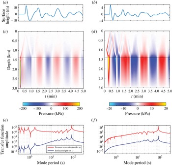
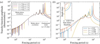
We will show that background stratification and non-equilibrium bubble growth and resorption (BGR) of primary volatile species are both heavily imprinted on the eigenmodes of volcanic conduits and on the excitation of these modes by internal volumetric sources and external forces. In § 2 we present a theoretical description of unsteady flow in an axisymmetric column of inviscid magma that accounts for depth variations in fluid properties and conduit width as well as non-equilibrium BGR. We linearize the equations of motion, and examine wave solutions in the context of a WKBJ approximation where background fluid properties can be assumed constant over several wavelengths (§ 3). This analysis, while not generally applicable to the longest-period eigenmodes of volcanic conduits, permits identification of key dimensionless parameters that quantify processes beyond those governing linear acoustic waves. We then develop a numerical method to solve the more general linearized problem in which background fluid properties vary with depth and conduit length is finite (§ 4). Finally, we connect our analysis of conduit eigenmodes to time-dependent excitation by numerically solving the linearized governing equations, exploring forces applied to the top of the conduit (e.g. rockfalls on the lava lake) and internal volumetric sources such as sudden additions of magma or collapse of gas slugs (§ 5). Results specific to each analysis type are presented in the respective sections, rather than at the end, for clarity. Future theoretical directions and applicability to volcanic seismicity and infrasound are summarized in § 6.
2 Governing equations
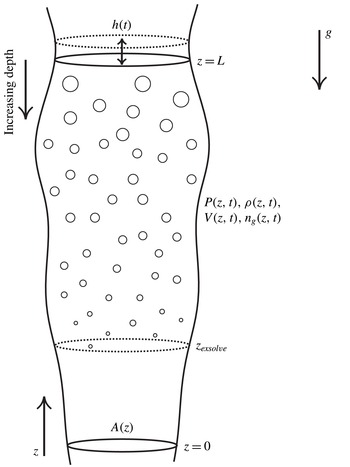
We consider one-dimensional, isothermal, axisymmetric and cross-sectionally averaged equations for the flow of two-phase bubbly magma through a conduit of cross-sectional area
 $A$
, expressed in an Eulerian description (figure 1). Relative motion between gas and liquid phases is neglected, with
 $V$
being the common vertical particle velocity of the gas and liquid phases. As discussed in § 2.4, this is likely a poor approximation in the description of the background state of the magma column, for the low-viscosity magmas of interest here, but is better justified for perturbations about the background state. We introduce the mixture density
 ${\it\rho}$
and mass fraction of exsolved gas
 $n_{g}$
; thus, the mass of exsolved gas per unit volume of the mixture is
 $n_{g}{\it\rho}$
and the mass of liquid per unit volume of the mixture is
 $(1-n_{g}){\it\rho}$
. Mass conservation for gas and liquid phases is then
 $$\begin{eqnarray}\displaystyle & \displaystyle \frac{\partial }{\partial t}(n_{g}{\it\rho}A)+\frac{\partial }{\partial z}(n_{g}{\it\rho}VA)={\it\rho}{\dot{m}}A, & \displaystyle\end{eqnarray}$$
 $$\begin{eqnarray}\displaystyle & \displaystyle \frac{\partial }{\partial t}[(1-n_{g}){\it\rho}A]+\frac{\partial }{\partial z}[(1-n_{g}){\it\rho}VA]=-{\it\rho}{\dot{m}}A, & \displaystyle\end{eqnarray}$$
respectively, where
 $z$
is vertical distance (positive up),
 $t$
is time, and
 ${\dot{m}}$
is the rate of mass conversion per unit total mass from the liquid phase to the gas phase (i.e. exsolution). Variables are implicitly assumed to depend on
 $z$
and
 $t$
unless stated otherwise. The conduit cross-sectional area is
 $A={\rm\pi}r^{2}$
for conduit radius
 $r$
. In this study, we neglect time-dependent changes in
 $A$
, as arise when deformable conduit walls are subject to pressure changes during oscillations of the magma column. That effect has been studied under steady-state conditions by Costa, Melnik & Sparks (Reference Costa, Melnik and Sparks2007), for example. It can also be important for determining wave speeds in fluid-filled conduits (Biot Reference Biot1956; White Reference White1983), though conduit wall deformation can be neglected when the fluid bulk modulus is far less than the shear modulus of the surrounding rock. That condition is certainly met in the upper portion of volcanic conduits, where exsolved gas substantially reduces the magma bulk modulus.
Equations (2.1) and (2.2) may equivalently be written in terms of mixture density and gas mass fraction:
 $$\begin{eqnarray}\displaystyle & \displaystyle \frac{\partial ({\it\rho}A)}{\partial t}+\frac{\partial ({\it\rho}VA)}{\partial z}=0, & \displaystyle\end{eqnarray}$$
 $$\begin{eqnarray}\displaystyle & \displaystyle \frac{\text{D}n_{g}}{\text{D}t}={\dot{m}}, & \displaystyle\end{eqnarray}$$
where
 $\text{D}/\text{D}t=\partial /\partial t+V\partial /\partial z$
is the material derivative. This form highlights conservation of mass of the mixture and further clarifies the interpretation of
 ${\dot{m}}$
as the gas exsolution rate.
An axisymmetric volcanic conduit of cross-sectional area
 $A(z)$
under the influence of gravity
 $g$
, filled with bubbly magma with pressure
 $P(z,t)$
, density
 ${\it\rho}(z,t)$
, vertical velocity
 $V(z,t)$
, and gas mass fraction
 $n_{g}(z,t)$
. Volatiles are completely dissolved below the exsolution depth
 $z=z_{\mathit{exsolve}}$
. The magma column extends from
 $z=0$
to
 $z=L$
in the background state. Magma oscillations move the upper surface to
 $z=L+h(t)$
, but in our linearized model boundary conditions are enforced on
 $z=L$
.

The momentum balance of the mixture is
 $$\begin{eqnarray}\displaystyle {\it\rho}\frac{\text{D}V}{\text{D}t}+\frac{\partial P}{\partial z}+{\it\rho}g+f=0, & & \displaystyle\end{eqnarray}$$
where
 $P$
is pressure,
 $g$
is gravity, and
 $f$
is the drag from shear stress on the conduit walls. In this initial study we assume inviscid magma and set
 $f=0$
.
With an eye towards future work, we remark that
 $f=8{\it\eta}V/r^{2}$
for fully developed, laminar Newtonian flow in a cylindrical conduit with radius
 $r$
and viscosity
 ${\it\eta}$
of the bubbly fluid. Alternative drag laws exist for turbulent or fragmented magma flows (e.g. Wilson & Head Reference Wilson and Head1981), plug flows with friction (e.g. Melnik & Sparks Reference Melnik and Sparks1999), or drag laws that incorporate non-Newtonian effects (e.g. Caricchi et al.
Reference Caricchi, Burlini, Ulmer, Gerya, Vassalli and Papale2007).
However, for the range of wave periods and conduit radii studied in this work, viscous effects are likely to be confined to boundary layers near the walls, and a simple parameterization in terms of the velocity
 $V$
at the current time is not possible. Flows become fully developed over time scales exceeding the momentum diffusion time across the conduit,
 ${\sim}{\it\rho}r^{2}/{\it\eta}$
. For the systems of interest here, we estimate
 ${\it\eta}\sim 10{-}1000$
Pa s,
 ${\it\rho}\sim 1000~\text{kg}~\text{m}^{-3}$
, and
 $r\sim 10$
m, leading to time scales of
 $10^{2}{-}10^{5}$
s. Thus, VLP oscillations with periods less than
 ${\sim}$
100 s have viscous effects confined to boundary layers.
We anticipate that calculations of wave speeds and eigenfrequencies from an inviscid model will be quite close to those from the viscous model, in the boundary layer limit (e.g. Lipovsky & Dunham Reference Lipovsky and Dunham2015). In this limit, the drag
 $f$
can be expressed in terms of a time convolution over the history of cross-sectionally averaged velocity
 $V$
. An alternative solution method is to solve the local, rather than cross-sectionally averaged, momentum balance in which
 $V$
depends also on radial distance. Because the main focus of the present work is on the effects on wave propagation of non-equilibrium BGR, stratification, and buoyancy, we neglect the effects of viscosity hereafter. However, a rigorous treatment of viscous dissipation in the context of this work is a logical and important next step, and one that is likely necessary to properly quantify the decay rates or quality factors of resonant modes.
We augment balance laws (2.1), (2.2) and (2.5) by an equation of state for mixture density of the form
 $$\begin{eqnarray}{\it\rho}={\it\rho}(P,n_{g}).\end{eqnarray}$$
This can be specifically stated in terms of the pressure-dependent densities of the gas and liquid phases,
 ${\it\rho}_{g}={\it\rho}_{g}(P)$
and
 ${\it\rho}_{l}={\it\rho}_{l}(P)$
, as (e.g. Wilson & Head Reference Wilson and Head1981)
 $$\begin{eqnarray}\frac{1}{{\it\rho}}=\frac{n_{g}}{{\it\rho}_{g}}+\frac{1-n_{g}}{{\it\rho}_{l}}.\end{eqnarray}$$
Here the gas mass fraction
 $n_{g}$
is not directly linked to the current pressure
 $P$
. But over sufficiently long time scales, a mixture of liquid melt and volatiles reaches a state in which
 $n_{g}$
reaches an equilibrium exsolved gas mass fraction,
 $n_{eq}(P)$
, due to the pressure-dependent solubility of volatiles (mostly H
 $_{2}$
O and CO
 $_{2}$
) in the melt. Equilibrium in this context is later referred to as thermodynamic equilibrium, which we distinguish from mechanical equilibrium of a magma column initially in a hydrostatic state (pressure gradient balancing weight). We will distinguish between these two types of equilibrium when it is not otherwise obvious from the context.
For later use, we quantify the sensitivity of
 $n_{eq}$
to
 $P$
by defining
 $$\begin{eqnarray}b=-\text{d}n_{eq}(P)/\text{d}P.\end{eqnarray}$$
As defined,
 $b\geqslant 0$
and might depend on
 $P$
. In the equilibrium limit, the mixture density is solely a function of pressure, and we define the equilibrium density as
 $$\begin{eqnarray}{\it\rho}_{eq}(P)={\it\rho}(P,n_{eq}(P)).\end{eqnarray}$$
In this work we consider waves and related oscillatory motions of magma in which pressure varies cyclically over a range of time scales. Adjustment to equilibrium requires a finite time, and consequently may not be complete at short time scales. This means we must consider
 $n_{g}$
as an additional field in the governing equations and introduce another equation describing the gas exsolution process.
Upon differentiating (2.6) following a fluid parcel, we obtain
 $$\begin{eqnarray}\frac{\text{D}{\it\rho}}{\text{D}t}=\frac{{\it\rho}}{K}\frac{\text{D}P}{\text{D}t}-a{\it\rho}\frac{\text{D}n_{g}}{\text{D}t},\end{eqnarray}$$
where
 $$\begin{eqnarray}K={\it\rho}(\partial {\it\rho}/\partial P)^{-1}\end{eqnarray}$$
is the bulk modulus of the fluid for fixed gas mass fraction and
 $$\begin{eqnarray}a=-{\it\rho}^{-1}(\partial {\it\rho}/\partial n_{g})\end{eqnarray}$$
quantifies the decrease in density associated with an increase in gas mass fraction. Both
 $K$
and
 $a$
are, in general, functions of
 $P$
and
 $n_{g}$
, and we have defined the dimensionless
 $a$
such that
 $a\geqslant 0$
. We can similarly define an equilibrium bulk modulus, relevant for quantifying the pressure dependence of density under sufficiently slow changes in pressure that
 $n_{g}=n_{eq}(P)$
, as
 $$\begin{eqnarray}K_{eq}={\it\rho}_{eq}(\text{d}{\it\rho}_{eq}/\text{d}P)^{-1}.\end{eqnarray}$$
Associated with
 $K$
and
 $K_{eq}$
are the sound speeds
 $$\begin{eqnarray}C=\sqrt{K/{\it\rho}}\quad \text{and}\quad C_{eq}=\sqrt{K_{eq}/{\it\rho}_{eq}},\end{eqnarray}$$
for propagation of acoustic waves under conditions of constant
 $n_{g}$
and of thermodynamic equilibrium, respectively.
Mass exchange between phases involves the dynamics of BGR. The effect of bubbles on bulk fluid properties and wave propagation has a long history of study generally (e.g. Silberman Reference Silberman1957; van Wijngaarden Reference van Wijngaarden1968; Commander & Prosperetti Reference Commander and Prosperetti1989) and in magmas specifically (e.g. Kieffer Reference Kieffer1977; Proussevitch & Sahagian Reference Proussevitch and Sahagian1996; Manga et al. Reference Manga, Castro, Cashman and Loewenberg1998; Lensky, Navon & Lyakhovsky Reference Lensky, Navon and Lyakhovsky2004; Kurzon et al. Reference Kurzon, Lyakhovsky, Navon and Chouet2011). Bubble growth in magma may be diffusively or viscously limited, depending on liquid phase composition, ambient pressure and temperature conditions, and melt viscosity (e.g. Proussevitch, Sahagian & Anderson Reference Proussevitch, Sahagian and Anderson1993; Navon, Chekhmir & Lyakhovsky Reference Navon, Chekhmir and Lyakhovsky1998; Huber et al. Reference Huber, Su, Nguyen, Parmigiani, Gonnermann and Dufek2014).
Although sophisticated models for the growth and dynamics of bubble populations exist, we employ a simple, single-parameter evolution equation (Woods Reference Woods1995) to isolate the interaction between non-equilibrium BGR and other effects:
 $$\begin{eqnarray}{\dot{m}}=-\frac{n_{g}-n_{eq}(P)}{{\it\tau}}.\end{eqnarray}$$
Equation (2.15) states that
 $n_{g}$
evolves towards its equilibrium value
 $n_{eq}(P)$
over the characteristic time scale
 ${\it\tau}$
. Such non-equilibrium BGR behaviour is well established in magmas (e.g. Gardner, Hilton & Carroll Reference Gardner, Hilton and Carroll1999), but
 ${\it\tau}$
is not well constrained experimentally. For the low-viscosity magmas of interest here, BGR is diffusively limited and the time scale
 ${\it\tau}$
measures the time for diffusive transport of volatiles through the liquid melt immediately surrounding the bubbles. Thus,
 ${\it\tau}$
depends on volatile diffusivity and also on bubble volume fraction (which sets whether spacing between bubbles or bubble radius is the relevant concentration gradient length scale), liquid composition (Yoshimura & Nakamura Reference Yoshimura and Nakamura2010), temperature, and volatile species (Zhang et al.
Reference Zhang, Xu, Zhu and Wang2007). Given the lack of observational constraints, we assume constant
 ${\it\tau}$
here to explore the basic phenomenology of non-equilibrium BGR on unsteady magma motions.
2.1 Linearized response of a fluid parcel
The response to small-amplitude perturbations about an equilibrium or steady-state solution can be studied using linearized versions of the governing equations. We thus write fluid variables velocity, pressure, density, and gas fraction as the sum of a background value, denoted with a bar, and a perturbation:
 $$\begin{eqnarray}[V,P,{\it\rho},n_{g}]=[\bar{v},\bar{p},\bar{{\it\rho}},\bar{n}]+[v,p,{\it\rho}^{\prime },n],\end{eqnarray}$$
and we linearize the governing equations around a background or base state. As mentioned earlier, perturbations in conduit area
 $A$
associated with elastic deformation of the conduit walls by pressure changes are neglected in this study.
We begin by considering a fluid parcel initially at thermodynamic equilibrium at pressure
 $P=\bar{p}$
, for which the initial gas mass fraction is
 $\bar{n}=n_{eq}(\bar{p})$
and the initial density is, from definition (2.9),
 $\bar{{\it\rho}}={\it\rho}_{eq}(\bar{p})$
. The more general problem of perturbations about a non-equilibrium background state is left for future work.
Linearizing the equation of state (2.6) yields
 $$\begin{eqnarray}\displaystyle {\it\rho}^{\prime } & = & \displaystyle \frac{\partial {\it\rho}}{\partial P}(P-\bar{p})+\frac{\partial {\it\rho}}{\partial n_{g}}(n_{g}-\bar{n})\nonumber\\ \displaystyle & = & \displaystyle \bar{{\it\rho}}(p/K-an),\end{eqnarray}$$
using the definitions of the bulk modulus
 $K$
in (2.11) and
 $a$
in (2.12). These and all subsequent coefficients are understood to be evaluated in the base state. The equilibrium gas mass fraction is similarly linearized,
 $$\begin{eqnarray}\displaystyle n_{eq}(P) & = & \displaystyle \bar{n}+\frac{\partial n}{\partial P}(P-\bar{p})\nonumber\\ \displaystyle & = & \displaystyle \bar{n}-bp,\end{eqnarray}$$
using (2.8) to define
 $b$
. In the context of this linearization, and assumption of perturbations about a state of thermodynamic equilibrium, the evolution equation (2.15) is
 $$\begin{eqnarray}{\dot{m}}=-\frac{n+bp}{{\it\tau}}.\end{eqnarray}$$
Similarly, the equilibrium density (2.9) is linearized:
 $$\begin{eqnarray}\displaystyle {\it\rho}_{eq}(P) & = & \displaystyle \bar{{\it\rho}}+\frac{\text{d}{\it\rho}_{eq}}{\text{d}P}(P-\bar{p})\nonumber\\ \displaystyle & = & \displaystyle \bar{{\it\rho}}+\frac{\bar{{\it\rho}}}{K}(1+abK)p=\bar{{\it\rho}}\left(1+\frac{p}{K_{eq}}\right)\!,\end{eqnarray}$$
using (2.13) and the identity
 $$\begin{eqnarray}\frac{1}{K_{eq}}=\frac{1}{K}+ab.\end{eqnarray}$$
Taking the total time derivative of (2.17), and making use of the equilibrium variables and the linearized evolution equation in (2.18)–(2.21), we eliminate
 $n$
and obtain a single equation describing the evolution of density under conditions of changing pressure:
 $$\begin{eqnarray}\frac{\text{D}{\it\rho}}{\text{D}t}=\frac{\bar{{\it\rho}}}{K}\frac{\text{D}P}{\text{D}t}-\frac{{\it\rho}-{\it\rho}_{eq}(P)}{{\it\tau}},\end{eqnarray}$$
or in terms of density and pressure perturbations,
 $$\begin{eqnarray}\frac{\text{D}{\it\rho}^{\prime }}{\text{D}t}=\frac{\bar{{\it\rho}}}{K}\frac{\text{D}p}{\text{D}t}-\frac{{\it\rho}^{\prime }-\bar{{\it\rho}}p/K_{eq}}{{\it\tau}}.\end{eqnarray}$$
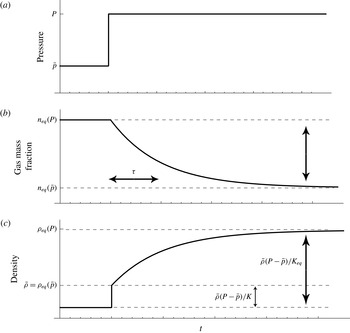
The significance of the two terms on the right-hand side of (2.22) or (2.23) can be understood by considering the response of the fluid parcel to a step increase in pressure (figure 2). That increase in pressure compresses both the gas and liquid phases, leading to an instantaneous increase in density described by the first term and quantified via the bulk modulus
 $K$
. Mass exchange between the phases is negligible during this initial compression. However, the increase in pressure alters the equilibrium solubility and drives volatiles back into the melt over the time scale
 ${\it\tau}$
. The second term captures this mass transfer and the associated reduction in mixture density towards the new, larger, equilibrium density.
Response of gas mass fraction
 $n$
and density
 ${\it\rho}$
to a step increase in pressure from (2.4) and (2.22). Gas fraction relaxes to a new equilibrium value over time scale
 ${\it\tau}$
, while density changes include both the instantaneous response due to fluid compression and slower relaxation response from mass exchange between phases.

2.2 Energetics of a fluid parcel
Introduction of a finite adjustment time
 ${\it\tau}$
necessarily implies energy dissipation. To illustrate this, and to prepare ourselves for later discussion of the energy balance for waves in magmatic conduits, we first consider the energetics of a fluid parcel. In the context of our linearized model, the rate of work per unit reference volume of fluid done by the pressure change
 $p$
is
 $$\begin{eqnarray}-\frac{p}{1/\bar{{\it\rho}}}\frac{\text{D}(1/{\it\rho})}{\text{D}t}=\frac{p}{\bar{{\it\rho}}}\frac{\text{D}{\it\rho}^{\prime }}{\text{D}t},\end{eqnarray}$$
where
 $1/{\it\rho}$
is the specific volume. With no addition of heat, the first law of thermodynamics states that the work done on the fluid parcel is equal to the change in internal energy. Here we show that the internal energy change consists of a recoverable part, the free energy associated with compression of the fluid, and dissipation from non-equilibrium BGR. We anticipate that the free energy per unit reference volume will be
 $p^{2}/2K$
under non-equilibrium conditions (when mass exchange is negligible) and
 $p^{2}/2K_{eq}$
under equilibrium conditions.
Substituting the linearized evolution equation (2.23) into (2.24) and using the identity (2.21), we obtain
 $$\begin{eqnarray}\frac{p}{\bar{{\it\rho}}}\frac{\text{D}{\it\rho}^{\prime }}{\text{D}t}=\frac{\text{D}}{\text{D}t}\left[\frac{p^{2}}{2K}+\frac{({\it\rho}^{\prime }-\bar{{\it\rho}}p/K)^{2}}{2ab\bar{{\it\rho}}^{2}}\right]+\frac{({\it\rho}^{\prime }-\bar{{\it\rho}}p/K_{eq})^{2}}{ab\bar{{\it\rho}}^{2}{\it\tau}}.\end{eqnarray}$$
The quantity in brackets is the total free energy density associated with compression of the fluid. The first part,
 $p^{2}/2K$
, is the non-equilibrium free energy density, which is the only contribution in the absence of mass exchange (in which case
 ${\it\rho}^{\prime }=\bar{{\it\rho}}p/K$
). The second part thus corresponds to an additional contribution to the free energy that arises as mass transfer lowers the fluid bulk modulus from
 $K$
towards
 $K_{eq}$
and additional work is done by pressure acting on the fluid parcel. The last term on the right-hand side of (2.25) is the rate of energy dissipation per unit reference volume. It is evident that dissipation occurs only when conditions depart from equilibrium. During equilibrium,
 ${\it\rho}^{\prime }=\bar{{\it\rho}}p/K_{eq}$
and dissipation vanishes. When BGR is limited by the ability of bubbles to expand or contract in a viscous melt, this energy loss is the usual viscous dissipation. Dissipation can also arise from diffusive processes (e.g. Landau & Lifshitz Reference Landau and Lifshitz1959, Ch. VI), such as when unequal chemical potentials drive transport of volatiles through the melt towards or away from the bubble walls.
We can also rewrite (2.25) by eliminating the density perturbation
 ${\it\rho}^{\prime }$
in favour of the gas mass fraction perturbation
 $n$
using (2.17):
 $$\begin{eqnarray}\frac{p}{\bar{{\it\rho}}}\frac{\text{D}{\it\rho}^{\prime }}{\text{D}t}=\frac{\text{D}}{\text{D}t}\left(\frac{p^{2}}{2K}+\frac{an^{2}}{2b}\right)+\frac{a(n+bp)^{2}}{b{\it\tau}}.\end{eqnarray}$$
The terms have the same interpretation, as
 $n=0$
in the absence of mass exchange and
 $n=-bp$
under equilibrium conditions. Furthermore, it is straightforward to verify that under equilibrium conditions the two free energy terms combine to
 $p^{2}/2K_{eq}$
, the equilibrium free energy density, as anticipated.
2.3 Perturbations about magmastatic base state
Having examined the response of an isolated fluid parcel, we now turn our attention to the response of the magma column. For all subsequent analysis we consider perturbations around a specific base state in which the magma is in both thermodynamic and mechanical equilibrium in the presence of a gravitational field. We refer to this as the magmastatic base state, for which
 $$\begin{eqnarray}\displaystyle & \bar{v}=0, & \displaystyle\end{eqnarray}$$
 $$\begin{eqnarray}\displaystyle & \displaystyle \frac{\text{d}\bar{p}}{\text{d}z}=-\bar{{\it\rho}}g, & \displaystyle\end{eqnarray}$$
 $$\begin{eqnarray}\displaystyle & \bar{n}=n_{eq}(\bar{p}), & \displaystyle\end{eqnarray}$$
and hence from (2.29), with the definition (2.9),
 $$\begin{eqnarray}\bar{{\it\rho}}={\it\rho}_{eq}(\bar{p}).\end{eqnarray}$$
The magmastatic state implies a vertical density stratification that can be obtained by differentiating (2.30) with respect to
 $z$
and using (2.13), (2.14) and (2.28):
 $$\begin{eqnarray}\frac{\text{d}\bar{{\it\rho}}}{\text{d}z}=-\frac{\bar{{\it\rho}}g}{C_{eq}^{2}}.\end{eqnarray}$$
Similarly, differentiating (2.29) with respect to
 $z$
and using (2.8) and (2.28) yields
 $$\begin{eqnarray}\frac{\text{d}\bar{n}}{\text{d}z}=\bar{{\it\rho}}gb.\end{eqnarray}$$
Stratified fluids exhibit oscillations for which the restoring force is gravity, especially at length scales exceeding the scale height for stratification,
 $C_{eq}^{2}/g$
(Lighthill Reference Lighthill1978). To quantify these oscillations, we define the buoyancy or Brunt–Väisälä frequency
 $$\begin{eqnarray}N_{b}=\sqrt{-\frac{g}{\bar{{\it\rho}}}\frac{\text{d}\bar{{\it\rho}}}{\text{d}z}}=\frac{g}{C_{eq}}.\end{eqnarray}$$
This definition of the buoyancy frequency is valid when fluid compressibility is negligible. As we later show, this is an appropriate approximation in our problem at wavelengths that are much greater than the scale height.
Introducing the magmastatic base state into the linearized governing equations reveals that there are only three linearly independent variables. This can be seen by taking the linearized material derivative of (2.17):
 $$\begin{eqnarray}\frac{1}{\bar{{\it\rho}}}\left(\frac{\partial {\it\rho}^{\prime }}{\partial t}+v\frac{\text{d}\bar{{\it\rho}}}{\text{d}z}\right)=\frac{1}{K}\left(\frac{\partial p}{\partial t}+v\frac{\text{d}\bar{p}}{\text{d}z}\right)-a\left(\frac{\partial n}{\partial t}+v\frac{\text{d}\bar{n}}{\text{d}z}\right)\!.\end{eqnarray}$$
From (2.28), (2.31) and (2.32), and the identity (2.21),
 $$\begin{eqnarray}\frac{1}{\bar{{\it\rho}}}\frac{\text{d}\bar{{\it\rho}}}{\text{d}z}=\frac{1}{K}\frac{\text{d}\bar{p}}{\text{d}z}-a\frac{\text{d}\bar{n}}{\text{d}z},\end{eqnarray}$$
so all the advection terms (those involving
 $v$
) in (2.34) cancel. We can then integrate (2.34) in time at fixed
 $z$
to find
 $$\begin{eqnarray}{\it\rho}^{\prime }=\bar{{\it\rho}}(p/K-an).\end{eqnarray}$$
This identity does not hold for more general base states in which a background flow is present.
Linearizing the momentum balance equation (2.5), mass balance equation (2.3), and BGR equation (2.4) yields
 $$\begin{eqnarray}\displaystyle & \displaystyle \bar{{\it\rho}}\frac{\partial v}{\partial t}+\frac{\partial p}{\partial z}+{\it\rho}^{\prime }g=0, & \displaystyle\end{eqnarray}$$
 $$\begin{eqnarray}\displaystyle & \displaystyle \frac{1}{\bar{{\it\rho}}}\left(\frac{\partial {\it\rho}^{\prime }}{\partial t}+v\frac{\text{d}\bar{{\it\rho}}}{\text{d}z}\right)+\frac{1}{A}\frac{\partial (Av)}{\partial z}=0, & \displaystyle\end{eqnarray}$$
 $$\begin{eqnarray}\displaystyle & \displaystyle \frac{\partial n}{\partial t}+v\frac{\text{d}\bar{n}}{\text{d}z}+\frac{n+bp}{{\it\tau}}=0, & \displaystyle\end{eqnarray}$$
respectively. The following steps then simplify the governing equations: use (2.36) to eliminate
 ${\it\rho}^{\prime }$
in (2.37). Use (2.34) to replace the material derivative of
 ${\it\rho}^{\prime }$
in (2.38) with material derivatives of
 $p$
and
 $n$
; then use (2.28) to eliminate
 $\text{d}\bar{p}/\text{d}z$
, and use (2.39) to eliminate the material derivative of
 $n$
. Finally use (2.32) to eliminate
 $\text{d}\bar{n}/\text{d}z$
in (2.39). What remains are three governing equations for
 $v,p$
, and
 $n$
:
 $$\begin{eqnarray}\displaystyle & \displaystyle \bar{{\it\rho}}\frac{\partial v}{\partial t}+\frac{\partial p}{\partial z}+\frac{\bar{{\it\rho}}g}{K}p-\bar{{\it\rho}}gan=0, & \displaystyle\end{eqnarray}$$
 $$\begin{eqnarray}\displaystyle & \displaystyle \frac{1}{K}\frac{\partial p}{\partial t}+\frac{1}{A}\frac{\partial (Av)}{\partial z}-\frac{\bar{{\it\rho}}g}{K}v+\frac{a}{{\it\tau}}\left(n+bp\right)=0, & \displaystyle\end{eqnarray}$$
 $$\begin{eqnarray}\displaystyle & \displaystyle \frac{\partial n}{\partial t}+\bar{{\it\rho}}gbv+\frac{n+bp}{{\it\tau}}=0. & \displaystyle\end{eqnarray}$$
In the limit of thermodynamic equilibrium (
 ${\it\tau}\rightarrow 0$
), often taken in quasi-steady volcanic conduit flow studies (e.g. Wilson & Head Reference Wilson and Head1981; Melnik & Sparks Reference Melnik and Sparks1999; Mastin Reference Mastin2002; Koyaguchi Reference Koyaguchi2005; Gonnermann & Manga Reference Gonnermann and Manga2006), these equations may be simplified (by utilizing the identities
 $n=-bp$
and (2.21)) to
 $$\begin{eqnarray}\displaystyle & \displaystyle \bar{{\it\rho}}\frac{\partial v}{\partial t}+\frac{\partial p}{\partial z}+\frac{\bar{{\it\rho}}g}{K_{eq}}p=0, & \displaystyle\end{eqnarray}$$
 $$\begin{eqnarray}\displaystyle & \displaystyle \frac{1}{K_{eq}}\frac{\partial p}{\partial t}+\frac{1}{A}\frac{\partial (Av)}{\partial z}-\frac{\bar{{\it\rho}}g}{K_{eq}}v=0. & \displaystyle\end{eqnarray}$$
2.4 Relative motion between gas and liquid
Having derived the linearized equations governing perturbations about the magmastatic state, we now discuss a basic assumption of this model, that of negligible relative motion between the gas and liquid phases. A full discussion and justification of this assumption is beyond the scope of this paper, but here we point out a few relevant issues. Relative motion is likely most important for the background state. Buoyancy drives upward motion of gas bubbles through the liquid melt, and out through the open vent and permeable conduit walls. Bubble dynamics plays a primary role in bulk magma motion, and may govern eruption style in low-viscosity settings such as we are studying (Houghton & Gonnermann Reference Houghton and Gonnermann2008). Gas loss will increase density, bulk modulus, and sound speed relative to the magmastatic state used in this study, especially in the shallow part of the conduit. Rise of gas bubbles will also cause departures from the hydrostatic balance condition (2.28). Furthermore, in some cases the gas volume fraction might increase to the point where interconnected pathways between bubbles develop to form a permeable bubble network (Kozono & Koyaguchi Reference Kozono and Koyaguchi2009), even in low-viscosity magmas (Rust & Cashman Reference Rust and Cashman2011).
Relative motion might also be important when considering perturbations about a base state. When that base state features upward gas flow, there will be advection terms in the governing equations. We suspect these terms will be negligible, given that the rise distance of even large bubbles or Darcian gas flow in a permeable network over VLP periods is small compared to vertical wavelengths of interest. Additionally, we can estimate the time scale over which perturbations in gas and liquid velocities equilibrate in response to interaction forces in the momentum balance equations. Assuming Stokes drag for the bubbles (providing an interaction force proportional to the difference in gas and liquid velocities), that adjustment time scale is of the order of
 $r_{B}^{2}{\it\rho}_{l}/{\it\eta}_{l}$
, where
 $r_{B}$
is the bubble radius,
 ${\it\rho}_{l}$
is liquid density, and
 ${\it\eta}_{l}$
is liquid viscosity (e.g. Landau & Lifshitz Reference Landau and Lifshitz1959). Even for large bubbles (
 $r_{B}\sim 10^{-2}$
m) in very low viscosity melt (
 ${\it\eta}_{l}/{\it\rho}_{l}\sim 10^{-2}$
m
 $^{2}$
s
 $^{-1}$
), the adjustment time scale is only
 ${\sim}$
1 s, still less than the
 ${\sim}$
30 s periods of the VLP events of interest. For more typical parameters, the adjustment time scale is many orders of magnitude smaller than periods of interest.
In any case, a rigorous examination of the role of relative motion, particularly in the base state, is warranted.
2.5 Boundary conditions
We now consider a conduit of length
 $L$
, extending between
 $z=0$
at depth to
 $z=L$
(prior to perturbations) at the surface. One boundary condition is required at each end of the conduit. Motivated by our interest in open-vent systems with lava lakes (such as Kilauea and Erebus), the top surface is assumed to be at constant atmospheric pressure:
 $$\begin{eqnarray}P(L+h(t),t)=P_{a}.\end{eqnarray}$$
While the surface position varies in time, the amplitude of its motions,
 $h(t)$
, is small compared to the height of the column
 $L$
. Thus, we expand the pressure at the surface in a Taylor series to first order:
 $$\begin{eqnarray}P(L+h(t),t)\approx P(L,t)+h(t)\left.\frac{\partial P}{\partial z}\right|_{z=L}.\end{eqnarray}$$
It suffices to evaluate the pressure gradient in the magmastatic state using (2.28), yielding the linearized boundary condition
 $$\begin{eqnarray}P(L,t)-\bar{{\it\rho}}(L)gh(t)=P_{a}.\end{eqnarray}$$
The evolution of the surface position
 $h(t)$
follows from the kinematic condition
 $$\begin{eqnarray}\text{d}h/\text{d}t=v(L+h(t),t),\end{eqnarray}$$
which is similarly linearized to
 $$\begin{eqnarray}\text{d}h/\text{d}t=v(L,t).\end{eqnarray}$$
The base of the conduit is connected to a magma reservoir. In this initial study we idealize such connection in terms of either constant-pressure or zero-velocity (no-flow) boundary conditions at the bottom of the conduit:
 $p(0,t)=0$
or
 $v(0,t)=0$
, respectively. In § 5.4 we introduce a simple model for the magma reservoir, and establish conditions under which the coupled model reduces to one of the simpler boundary conditions used in this work. We discuss possible more sophisticated models of the coupled system in § 6. In the examples that follow, except when stated otherwise, we use the constant-pressure condition.
To summarize, the linearized boundary conditions are
 $$\begin{eqnarray}\displaystyle & p(0,t)=0, & \displaystyle\end{eqnarray}$$
 $$\begin{eqnarray}\displaystyle & p(L,t)-\bar{{\it\rho}}(L)gh(t)=0, & \displaystyle\end{eqnarray}$$
and we must add (2.49) to governing equations (2.40)–(2.42).
2.6 Energy balance
In this section, we derive the balance of mechanical energy
 $E$
for a finite length column of fluid, in anticipation of the application to magmatic conduits. The energy balance is obtained by multiplying the momentum balance (2.40) by
 $Av$
and integrating over the conduit. After utilizing the other governing equations, properties of the base state, and boundary conditions, we obtain
 $$\begin{eqnarray}E=\int _{0}^{L}\left(\frac{\bar{{\it\rho}}v^{2}}{2}+\frac{p^{2}}{2K}+\frac{an^{2}}{2b}\right)A\,\text{d}z+\frac{A(L)\bar{{\it\rho}}(L)gh^{2}}{2},\end{eqnarray}$$
which evolves in time according to
 $$\begin{eqnarray}\frac{\text{d}E}{\text{d}t}=-\int _{0}^{L}\frac{a(n+bp)^{2}}{b{\it\tau}}A\,\text{d}z.\end{eqnarray}$$
The total energy is the sum of kinetic energy and several potential energy terms that appeared in our discussion of the energetics of a fluid parcel (2.25) and (2.26). The last term in (2.52) is the gravitational potential energy associated with motions of the free surface. As before, we refer to
 $p^{2}/2K$
as the non-equilibrium free energy density and
 $p^{2}/2K+an^{2}/2b$
as the total free energy density. The latter is always less than or equal to the equilibrium free energy density
 $p^{2}/2K_{eq}$
. The right-hand side of (2.53) is the energy dissipation rate from non-equilibrium BGR.
In the case of equilibrium BGR, the energy simplifies to
 $$\begin{eqnarray}E=\int _{0}^{L}\left(\frac{\bar{{\it\rho}}v^{2}}{2}+\frac{p^{2}}{2K_{eq}}\right)A\,\text{d}z+\frac{A(L)\bar{{\it\rho}}(L)gh^{2}}{2},\end{eqnarray}$$
and is conserved,
 $\text{d}E/\text{d}t=0$
.
Equation (2.53) establishes that perturbations to the magmastatic base state uniformly decay in time. Energy loss is due to non-equilibrium effects (the last term on the right-hand side of (2.53)). Although we assume inviscid flow here, had we included viscous effects and wall drag there would be an additional dissipation term appearing in the energy balance.
2.7 Magmatic application
We must specify an appropriate mixture equation of state and a gas solubility law to close our problem. For the magmatic systems of interest, the gas phase will follow an ideal gas law to a good approximation, and a linearized model for a compressible liquid is appropriate. Density is given by the mixture equation (2.7), with
 $$\begin{eqnarray}{\it\rho}_{g}(P)=\frac{P}{RT}\quad \text{and}\quad {\it\rho}_{l}(P)={\it\rho}_{liq}\left(1+\frac{P-P_{0}}{K_{liq}}\right)\!,\end{eqnarray}$$
with
 $R=462$
J kg
 $^{-1}$
K the ideal gas constant and
 $T=1273$
K a temperature representative of basaltic magma,
 ${\it\rho}_{liq}=3000$
kg m
 $^{-3}$
a reference magma liquid density,
 $K_{liq}=10$
GPa the liquid bulk modulus, and
 $P_{0}$
is a reference pressure about which the liquid density is linearized. In what follows we deal with a linearized form of this equation of state as in (2.17).
We assume at first that water is the only volatile species present, in which case equilibrium solubility
 $n_{eq}(P)$
approximately follows from Henry’s law,
 $$\begin{eqnarray}n_{eq}(P)=n_{t}-S_{w}\sqrt{P},\end{eqnarray}$$
with
 $n_{t}$
the total water mass fraction. Equation (2.56) can be modified to include nucleation and supersaturation effects (Woods Reference Woods1995).
 $S_{w}\approx 4\times 10^{-6}$
Pa
 $^{-1/2}$
is an empirical constant, which is an approximation to the equilibrium solubility of water in silicate melts. In general there are multiple volatile species present in magma, but water is nearly always the dominant volatile by at least an order of magnitude (Wallace Reference Wallace2005). Volatile exsolution is dominantly pressure-dependent, with single-phase fluid (no gas bubbles) above a critical pressure
 $P_{\mathit{exsolve}}$
. For Henry’s law and water the only volatile species,
 $P_{\mathit{exsolve}}=(n_{t}/S_{w})^{2}$
.
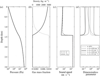
Figure 3 illustrates the variation of background variables with depth for the case of total water content
 $n_{t}=0.01$
. Spatial gradients in gas content, and therefore density and pressure, are most pronounced just above the depth of exsolution, defined as the value of
 $z$
for which
 $\bar{p}(z)=P_{\mathit{exsolve}}$
. Differences between equilibrium and non-equilibrium sound speeds are also largest at this transition. The scale height for background stratification (the length scale at and above which effects of gravity are non-negligible) is
 $C_{eq}^{2}/g\sim 25{-}500$
m between the depth of gas exsolution and the surface.
Depth dependence of background fluid properties in the magmastatic state, assuming total gas mass fraction
 $n_{t}=0.01$
. (a) Pressure
 $P$
, (b) density
 ${\it\rho}$
and gas mass fraction
 $n_{g}$
, (c) equilibrium and non-equilibrium sound speeds
 $C_{eq}$
and
 $C$
, and (d) depth distribution of the dimensionless parameters
 ${\it\gamma},{\it\alpha}$
, and
 ${\it\sigma}$
(3.5)–(3.7) for two representative wavenumbers and
 ${\it\tau}=1$
s. While
 ${\it\sigma}$
and
 ${\it\alpha}$
are not defined below the exsolution depth (at
 ${\approx}$
1420 m),
 ${\it\gamma}$
takes a small but finite value below exsolution (
 ${\it\gamma}=3\times 10^{-5}$
,
 $3\times 10^{-4}$
for
 $k=0.1$
, 0.01 m
 $^{-1}$
, respectively).

3 Eigenmodes: frozen coefficient analysis
Our next objective is to study the nature of waves and eigenmodes of vibration for perturbations about the magmastatic base state. The full problem, which involves substantial depth variations in properties, prohibits analytic analysis. We therefore first examine a simpler system by utilizing a short-wavelength, WKBJ-type approximation in which background fluid properties (the coefficients in the linearized governing equations) are frozen by evaluation at a reference pressure
 $\bar{p}$
. This is valid for perturbation wavelengths that are much shorter than the scale height characterizing variations in background coefficients, such as
 $\bar{{\it\rho}}/|\text{d}\bar{{\it\rho}}/\text{d}z|$
. While it is unlikely that this approximation will be of much utility in describing actual wave motions at the long periods of interest, this analysis provides substantial insight into the physics of waves in this system.
The governing equations (2.40)–(2.42) are non-dimensionalized using a wavenumber
 $k$
to provide the characteristic length scale and scalings appropriate for sound waves in the absence of gravity and mass exchange between the phases. The non-dimensional variables, denoted with an asterisk, are related to the dimensional variables via
 $$\begin{eqnarray}Uv^{\ast }=v,\quad \bar{{\it\rho}}CUp^{\ast }=p,\quad \frac{U}{Ca}n^{\ast }=n,\quad z^{\ast }=kz,\quad t^{\ast }=Ckt,\end{eqnarray}$$
with
 $U$
being a characteristic particle velocity. Note that
 $U$
simply sets the overall amplitude in this linearized problem, and consequently will not appear in any dimensionless parameter groups.
The dimensionless governing equations are
 $$\begin{eqnarray}\displaystyle & \displaystyle \frac{\partial v^{\ast }}{\partial t^{\ast }}+\frac{\partial p^{\ast }}{\partial z^{\ast }}+{\it\gamma}(p^{\ast }-n^{\ast })=0, & \displaystyle\end{eqnarray}$$
 $$\begin{eqnarray}\displaystyle & \displaystyle \frac{\partial p^{\ast }}{\partial t^{\ast }}+\frac{\partial v^{\ast }}{\partial z^{\ast }}-{\it\gamma}v^{\ast }+\frac{n^{\ast }+{\it\alpha}p^{\ast }}{{\it\sigma}}=0, & \displaystyle\end{eqnarray}$$
 $$\begin{eqnarray}\displaystyle & \displaystyle \frac{\partial n^{\ast }}{\partial t^{\ast }}+{\it\gamma}{\it\alpha}v^{\ast }+\frac{n^{\ast }+{\it\alpha}p^{\ast }}{{\it\sigma}}=0. & \displaystyle\end{eqnarray}$$
The three dimensionless groups are
 $$\begin{eqnarray}\displaystyle & \displaystyle {\it\gamma}=\frac{g}{C^{2}k}, & \displaystyle\end{eqnarray}$$
 $$\begin{eqnarray}\displaystyle & \displaystyle {\it\alpha}=abK=\frac{K}{K_{eq}}-1=\frac{N_{b}^{2}C^{2}}{g^{2}}-1, & \displaystyle\end{eqnarray}$$
 $$\begin{eqnarray}\displaystyle & \displaystyle {\it\sigma}=Ck{\it\tau}. & \displaystyle\end{eqnarray}$$
They have the following interpretation. The first,
 ${\it\gamma}$
, compares gravity and compressibility and appears in similar problems involving wave propagation in a compressible fluid in a gravitational field (e.g. Sells Reference Sells1965; Gill Reference Gill1982). When
 ${\it\gamma}\ll 1$
, gravity is negligible. The second,
 ${\it\alpha}$
, quantifies the difference between (thermodynamic) non-equilibrium and equilibrium fluid properties, with larger values of
 ${\it\alpha}$
signifying more substantial differences. The third,
 ${\it\sigma}$
, is the product of the angular frequency of a sound wave,
 $Ck$
, and the time scale
 ${\it\tau}$
governing bubble growth and resorption. When
 ${\it\sigma}\ll 1$
, bubble growth and resorption occur much faster than the cyclic changes in pressure and the gas and liquid phases are effectively in thermodynamic equilibrium. In the opposite,
 ${\it\sigma}\gg 1$
limit, there is negligible mass transfer between the phases.
The ranges of these dimensionless groups for a gas-poor magma are shown in figure 3(d) for several wavenumbers. It might be important to consider a larger range in
 ${\it\sigma}$
than plotted in figure 3, given the currently poor constraints on
 ${\it\tau}$
. Further discussion of
 ${\it\tau}$
appears in § 6.
We note here that the linear operator in this problem is non-normal except in special limits. This means that eigenmodes are not necessarily orthogonal, and raises the possibility of transient growth and other effects associated with non-normal operators (Trefethen et al. Reference Trefethen, Trefethen, Reddy and Driscoll1993; Trefethen & Embree Reference Trefethen and Embree2005). However, later calculations show that the longest-period eigenmodes are very close to orthogonal, and our limited set of time-domain simulations for representative excitation processes has not revealed transient growth effects. Therefore, we defer a comprehensive investigation of non-normality to future work.
The homogeneous, constant-coefficient governing equations can now be reduced to a set of algebraic equations by seeking modal solutions with
 $\text{e}^{\text{i}kz+st}$
dependence, or in dimensionless form
 $$\begin{eqnarray}[v^{\ast },p^{\ast },n^{\ast }]=[\mathscr{V},\mathscr{P},\mathscr{N}]\exp (\text{i}z^{\ast }+s^{\ast }t^{\ast }),\end{eqnarray}$$
where
 $s^{\ast }=s/Ck$
. The imaginary part of
 $s^{\ast }$
is the phase velocity normalized by
 $C$
; the real part of
 $s^{\ast }$
, which is non-positive, is the decay rate normalized by
 $Ck$
, the angular frequency of a sound wave propagating at speed
 $C$
.
Taking the determinant of the coefficient matrix of this system yields a characteristic equation for eigenvalues
 $s^{\ast }$
:
 $$\begin{eqnarray}1+{\it\gamma}^{2}(1+{\it\alpha})^{2}+{\it\sigma}[{\it\gamma}^{2}(1+{\it\alpha})+1]s^{\ast }+(1+{\it\alpha})s^{\ast 2}+{\it\sigma}s^{\ast 3}=0.\end{eqnarray}$$
We explore the solutions to this characteristic equation for the parameter space defined by
 ${\it\gamma},{\it\alpha}$
, and
 ${\it\sigma}$
by first focusing on three important limits. Wave propagation in the absence of gravity, stratification, and non-equilibrium BGR occurs at speed
 $C$
, or equivalently
 $s^{\ast }=\mp \text{i}$
(with the
 $\mp$
referring to wave propagation in the
 $\pm z$
direction for positive
 $k$
). Similarly, wave propagation in the absence of gravity and stratification, but under equilibrium conditions occurs at speed
 $C_{eq}$
, or
 $s^{\ast }=\mp \text{i}/\sqrt{1+{\it\alpha}}$
. In both of these limits, propagation is non-dispersive. Finally, oscillations at the Brunt–Väisälä frequency
 $N_{b}$
defined in (2.33) correspond to
 $s^{\ast }=\mp \text{i}{\it\gamma}\sqrt{1+{\it\alpha}}$
. Note that the oscillation frequency is independent of the wavenumber
 $k$
in this case, so that while it is possible to define a phase velocity (which diverges as
 $k\rightarrow 0$
), the group velocity is zero.
The cubic characteristic equation (3.9) has three solutions. The energy analysis in § 2.6 guarantees stability; that is,
 $\text{Re}[s^{\ast }]\leqslant 0$
. One solution is always purely real and less than or equal to zero. This solution is consequently non-oscillatory (i.e. non-propagating) and is associated with the adjustment of the system towards equilibrium through BGR. The other two solutions generally take the form of propagating waves with
 $\text{Im}[s^{\ast }]\neq 0$
, though, as we later show, energy dissipation from non-equilibrium effects can cause these waves to become overdamped and non-propagating. We begin our study of the effects of gravity and non-equilibrium BGR by taking two limits, before turning to the full problem.
3.1 Zero-gravity limit
If
 ${\it\gamma}=0$
, gravitational restoring force in the momentum balance (3.2) is eliminated, as is stratification in the magmastatic state. Stratification enters through advection terms in (3.3) and (3.4). This limit is obtained by taking
 $g\rightarrow 0$
for finite wavenumber
 $k$
(for example by considering a horizontal instead of vertical conduit) such that
 ${\it\sigma}$
remains finite. Non-equilibrium BGR provides the only deviation from standard acoustics, where the solutions are well known (undamped waves propagating up and down the conduit at speed
 $C$
, equipartition between kinetic and non-equilibrium free energy, Lighthill Reference Lighthill1978). The characteristic equation reduces to
 $$\begin{eqnarray}1+{\it\sigma}s^{\ast }+(1+{\it\alpha})s^{\ast 2}+{\it\sigma}s^{\ast 3}=0.\end{eqnarray}$$
This cubic equation has three roots, one of which is always real and non-positive. This root quantifies the rate of mass exchange between the phases. The other two solutions correspond to waves, and there are two limits of interest. In the high-frequency limit there is not time for mass exchange over a wave period, so
 ${\it\sigma}\rightarrow \infty$
, (3.10) reduces to
 $s^{\ast }(1+s^{\ast 2})=0$
and the wave modes are
 $s^{\ast }=\mp \text{i}$
. These waves are undamped and propagate at the non-equilibrium sound speed
 $C$
without dispersion. In the low-frequency limit,
 ${\it\sigma}\rightarrow 0$
and thermodynamic equilibrium is maintained over a wave period. Equation (3.10) reduces to
 $1+(1+{\it\alpha})s^{\ast 2}=0$
and propagation occurs at the equilibrium sound speed
 $C_{eq}$
with
 $s^{\ast }=\mp \text{i}/\sqrt{1+{\it\alpha}}$
.
The differences between equilibrium and non-equilibrium fluid properties, as measured by
 ${\it\alpha}$
, become most significant as the gas exsolution pressure is approached (figure 3). Although wavelike solutions for most of the parameter space come in complex conjugate pairs, there are parameters for which all roots of (3.10) are purely real and negative. This overdamped regime of perturbations coincides with the transition between equilibrium and non-equilibrium wave propagation, and occurs where the discriminant of (3.10) is positive, or where
 $$\begin{eqnarray}-4{\it\sigma}^{4}+{\it\sigma}^{2}({\it\alpha}(20+{\it\alpha})-8)-4(1+{\it\alpha})^{3}\geqslant 0.\end{eqnarray}$$
The quadratic equation in
 ${\it\sigma}^{2}$
may only be satisfied for
 ${\it\alpha}\geqslant 8$
, which for realistic parameters is generally restricted to a narrow region above the exsolution depth. We note that similar overdamped behaviour is found in other two-phase models that consider relative motion between phases (e.g. Bercovici & Michaut Reference Bercovici and Michaut2010).
3.2 Long-wavelength limit
We now take
 ${\it\gamma}\rightarrow \infty$
(by taking
 $k\rightarrow 0$
with finite
 $g$
), which corresponds to a long-wavelength limit in which the effects of gravity and stratification dominate. The pressure gradient term is negligible in the momentum balance and the velocity divergence term is negligible in the mass balance equation. Instead, terms involving
 $g$
become important. These describe the gravitational restoring force associated with density perturbation in the momentum balance, and the change in density arising from advection through a stratified background state. Compressibility is negligible. The purely real root approaches
 $s^{\ast }=-(1+{\it\alpha})/{\it\sigma}$
, which moves off towards
 $-\infty$
in the
 ${\it\sigma}\rightarrow 0$
thermodynamic equilibrium limit (corresponding to instantaneous adjustment to equilibrium).
For the two wavelike solutions, we anticipate (and can verify a posteriori) that
 $s^{\ast }$
is
 $O({\it\gamma})$
. Removing the purely real root and dropping all but the highest-order terms in
 ${\it\gamma}$
, the dispersion relation reduces to
 $$\begin{eqnarray}{\it\gamma}^{2}(1+{\it\alpha})+s^{\ast 2}=0,\end{eqnarray}$$
irrespective of the value of
 ${\it\sigma}$
. The solutions,
 $s^{\ast }=\mp \text{i}{\it\gamma}\sqrt{1+{\it\alpha}}$
, describe undamped oscillations at the Brunt–Väisälä frequency
 $N_{b}$
defined in (2.33).
3.3 General case
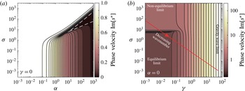
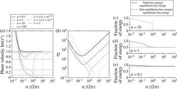
We now return to the general case. Figure 4 presents the wavelike solutions to the dispersion relation (3.9). In the
 ${\it\gamma}=0$
limit,
 ${\it\sigma}\gg 1$
is the non-equilibrium BGR regime, while
 ${\it\sigma}\ll 1$
is the equilibrium BGR regime (figure 4
a). The value
 ${\it\alpha}$
determines the extent to which equilibrium and non-equilibrium regimes are distinct, and as well whether there is an overdamped regime (dashed white contour). Figure 4(b) examines another slice through this parameter space, at
 ${\it\alpha}=10$
for non-zero
 ${\it\gamma}$
, and we see that for large
 ${\it\gamma}$
, phase velocity follows the gravity wave limit, independent of
 ${\it\sigma}$
.
(a) Dimensionless phase velocity
 $\text{Im}[s^{\ast }]$
in the zero-gravity limit (
 ${\it\gamma}=0$
) described by (3.10), as a function of
 ${\it\alpha}$
and
 ${\it\sigma}$
. Within the dashed white contour, solutions are overdamped and non-propagating. The contour is defined by (3.11). The phase velocity is determined primarily by
 ${\it\alpha}$
, which quantifies differences between the equilibrium and non-equilibrium sound speeds
 $C_{eq}$
and
 $C$
. (b) Regime diagram for fixed
 ${\it\alpha}=10$
as a function of
 ${\it\gamma}$
and
 ${\it\sigma}$
, showing the parameter dependence of the three propagation regimes. The red curve is the trajectory through parameter space as wavenumber in decreased with all other properties fixed; solutions along this curve are plotted in figure 5.

In figure 5 we explore these three propagation regimes as wavenumber is varied. Changing
 $k$
alters both
 ${\it\sigma}$
and
 ${\it\gamma}$
, while leaving
 ${\it\alpha}$
and
 ${\it\sigma}/{\it\gamma}$
fixed. These three regimes are plotted explicitly for several choices of
 ${\it\alpha}$
in figure 5(a), with thin lines corresponding to the phase velocity limits discussed above.
Effect of varying wavenumber while holding all other properties fixed. This changes both
 ${\it\sigma}$
and
 ${\it\gamma}$
with their ratio held fixed, as shown in figure 4 (and see text). (a) Phase velocity
 $s^{\ast }$
of eigenmodes as a function of
 ${\it\sigma}/(2{\rm\pi})$
, for several choices of
 ${\it\alpha}$
. Thin lines outline the three wave propagation regimes: non-equilibrium BGR, equilibrium BGR, and gravity wave limits. For
 ${\it\alpha}=100$
we see a region of overdamped waves (zero phase velocity). For all others there is a symmetric conjugate wave (not plotted). (b) Quality factor
 $Q$
(3.13) for the cases in (a). (c–e) Non-equilibrium (dashed) and total (solid) free energy density, relative to equilibrium free energy (§ 2.2) for the modes in (a). Ratio of non-equilibrium to equilibrium free energy density equals
 $K_{eq}/K=(1+{\it\alpha})^{-1}$
. Differences between total and equilibrium free energy indicate departure from thermodynamic equilibrium.

Even when there are no overdamped modes, the transitional regime around
 ${\it\sigma}/(2{\rm\pi})\sim 1$
, where the wave period is similar to
 ${\it\tau}$
, represents the most damped part of parameter space. As figure 5(a,b) shows with a family of curves, if we define a quality factor (damping over one oscillation cycle) for propagating modes as
 $$\begin{eqnarray}Q=\frac{\text{Im}(s)}{2\text{Re}(s)},\end{eqnarray}$$
the least damped (highest Q) modes correspond to the short- and long-wavelength limits. The region around
 ${\it\sigma}/(2{\rm\pi})\sim 1$
is the most highly damped, optimizing the dissipation from non-equilibrium phase exchange (2.53). Figure 5(a) plots only one of the complex conjugate roots, except for the region of overdamped propagation for large
 ${\it\alpha}$
(in which there are not conjugate roots). Curves in figure 5(a,b) can also be interpreted as the dispersion relation for coefficients frozen at increasing depths in the conduit (pressures) as
 ${\it\alpha}$
increases (figure 3
d).
 ${\it\gamma}$
increases by a factor of
 ${\sim}50$
from
 ${\it\alpha}=0.1$
to
 ${\it\alpha}=100$
at fixed wavenumber.
3.4 Energetics
For each of the solutions of the characteristic equation (3.9) at a given wavelength, we can evaluate the partition of total energy into kinetic and potential energy. The gravitational energy term does not appear, as the domain is periodic. Figure 5(c–e) plots contributions to the potential energy of the propagating modes from panel (a) (
 ${\it\alpha}=0.1,1,10$
) according to the partitioning defined by (2.52).
For wave periods much smaller than
 ${\it\tau}$
(
 ${\it\sigma}\gg 1$
), there is negligible BGR over a wave period and energy is equally partitioned between kinetic and non-equilibrium free energy, as is the case for simple acoustics. For
 ${\it\sigma}\ll 1$
, BGR keeps the system in thermodynamic equilibrium and the mixture is more compressible than in the non-equilibrium case; total energy is equally partitioned between kinetic and equilibrium free energy (2.54). Figure 5(c–e) illustrates this transition in fluid compressibility, and hence free energy, and highlights its dependence on the time scale of the wave motion relative to
 ${\it\tau}$
as quantified through
 ${\it\sigma}$
. It is also clear that
 ${\it\alpha}$
quantifies the difference in fluid compressibility; as
 ${\it\alpha}\rightarrow 0$
, the difference between non-equilibrium and equilibrium free energy becomes negligible.
4 Eigenmodes: depth-dependent properties
One of the defining aspects of even the simplest volcanic conduit systems is the strong variation of fluid properties with depth. Below the depth of gas exsolution, the fluid is single phase, with properties such as density and compressibility given by pure liquid values. Above exsolution, gas mass fraction increases nonlinearly as the surface is approached. In this region we expect the volume distribution of gas bubbles to vary in space along with the degree of non-equilibrium BGR. Additionally, conduit radius may not be constant with depth. These features imply spatially varying coefficients in our governing equations, so the eigenmodes are no longer Fourier modes, and the eigenvalue problem must be solved numerically.
4.1 Numerical method
We therefore develop a numerical method that can be used to both solve the eigenvalue problem and study excitation of these eigenmodes in the time domain. We return to dimensional governing equations, but now discretize in space using finite differences. Specifically, a field such as
 $v(z,t)$
is discretized on a finite domain
 $0\leqslant z\leqslant L$
at a set of
 $M+2$
possibly non-uniformly spaced grid points
 $z_{i}$
. The discontinuity in properties at the gas exsolution depth is handled using split nodes, that is, a pair of collocated points, one on either side of the material interface, with appropriate conditions enforcing mass and momentum balance across the interface. A field such as
 $v(z,t)$
is approximated at the grid points, with the grid values stored in a vector
 $\boldsymbol{v}(t)$
having components
 $v_{i}(t)\approx v(z_{i},t)$
.
We use summation-by-parts (SBP) finite differences (Kreiss & Scherer Reference Kreiss, Scherer and de Boor1974, Reference Kreiss and Scherer1977; Strand Reference Strand1994; Gustafsson, Kreiss & Oliger Reference Gustafsson, Kreiss and Oliger1995). Boundary conditions (and interface conditions across the material interface at the exsolution depth) are enforced weakly with the simultaneous approximation term (SAT) method (Carpenter, Gottlieb & Abarbanel Reference Carpenter, Gottlieb and Abarbanel1994). With the SBP–SAT framework (e.g. Svard & Nordstrom Reference Svard and Nordstrom2014) we can construct a discrete energy balance that closely mimics the continuous energy balance (2.53) and prove that numerical solutions are both stable and high-order accurate. The examples shown below use a globally fifth-order-accurate difference operator. Derivation of the discrete version of governing equations (2.40)–(2.42) and (2.49), boundary and interface conditions, and the energy balance (2.53) are presented in appendix A.
This method is first used to solve the eigenproblem that arises after Laplace transforming, with Laplace parameter
 $s$
, the semi-discrete governing equations:
 $$\begin{eqnarray}s\tilde{\boldsymbol{u}}=\unicode[STIX]{x1D63D}\tilde{\boldsymbol{u}},\end{eqnarray}$$
where
 $\boldsymbol{u}(t)=[v_{0}(t),\ldots ,v_{M+2}(t),p_{0}(t),\ldots ,p_{M+2}(t),n_{0}(t),\ldots ,n_{M+2}(t),h(t)]^{\text{T}}$
is a column vector of velocity, pressure perturbation, and gas fraction perturbation at the grid points along with the free surface displacement
 $h$
, and
 $$\begin{eqnarray}\tilde{\boldsymbol{u}}(s)=\int _{0}^{\infty }\boldsymbol{u}(t)\text{e}^{-st}\,\text{d}t\end{eqnarray}$$
defines the Laplace transform.
 $\unicode[STIX]{x1D63D}$
is a
 $3(M+2)+1\times 3(M+2)+1$
matrix containing spatially variable fluid properties evaluated at the grid points, the finite difference operator, and penalty terms that enforce interface and boundary conditions (see appendix A for details). There are
 $3(M+2)+1$
eigenvalues, which we store for later use in the diagonal matrix
 ${\it\bf\Lambda}$
.
Diagonalization of
 $\unicode[STIX]{x1D63D}$
defines the eigenmodes of the system, with the corresponding eigenvalues characterizing the oscillation frequencies and decay rates of modes. In contrast to the frozen coefficient case, where eigenmodes took the form of Fourier modes, eigenmodes of the finite conduit exhibit a complex spatial structure that reflects the strong gradients in background fluid properties. In particular, a large impedance contrast at the exsolution interface serves to segment the conduit into two parts, with significantly different properties due to the presence of bubbles and increased compressibility in the upper portion of the conduit.
4.2 Eigenmode families
Results for a 3 km length conduit with
 $n_{t}=0.01$
,
 $p=0$
bottom boundary condition, and three choices of
 ${\it\tau}$
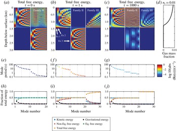
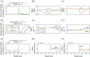
are shown in figures 6 and 7. The eigenfunction amplitudes are only defined up to an arbitrary constant. We choose this constant in figure 6 so that total free energy density has unit maximum amplitude, which facilitates comparison of mode families. For figure 7 the constant is chosen to make the total energy of each mode equal to 10 kJ. Note that
 $n$
is not defined, and hence not plotted, below the exsolution depth in figure 7.
Families of eigenmodes for (a,e,h)
 ${\it\tau}=0$
s (equilibrium BGR), (b,f,i)
 ${\it\tau}=1$
s, (c,g,j)
 ${\it\tau}=1000$
s (non-equilibrium BGR). Ten longest-period eigenmodes in each family are shown, with the normalization and family naming scheme described in the text. (d) Background gas mass fraction, showing segmentation of conduit into bubbly magma above exsolution and liquid melt below. (a–c) Spatial distribution of total free energy density. Bright colours indicate regions where magma is compressed or expanded. (e–g) Mode period, dots coloured by decay rate. (h–j) Energetics. (a,e,h) shows contributions to potential energy from equilibrium free energy (which equals total free energy) and gravitational potential energy. In panels (b,f,i,c,g,j), potential energy is divided into total free energy and gravitational potential energy; also shown is non-equilibrium free energy (which differs from total free energy when BGR is appreciable over a mode period). White arrows in (b) refer to modes plotted in figure 7.

Three eigenmodes, labelled with white arrows in figure 6(b), for
 $p=0$
bottom boundary condition and
 ${\it\tau}=1$
s, with normalization described in text. Modes are uniformly scaled to reflect typical excitation amplitudes presented here. (a,d,g) Kinetic and free energy density. (b,e,h) and (c,f,i) Eigenfunctions for pressure perturbation, velocity, and exsolved gas mass fraction perturbation. Particular labelled modes have been uniformly scaled for visualization purposes.

We find three families of modes, labelled in figure 6(a–c). Family I contains the longest-period modes of the conduit. Most of these modes, with the exception of the fundamental mode discussed below, are localized primarily above the exsolution depth. Family II contains shorter-period eigenmodes. When
 ${\it\tau}$
is comparable to the mode periods (
 ${\sim}$
1 s in this example), these modes exhibit dominant or even exclusive spatial localization below the exsolution depth. Family III exists only for non-zero
 ${\it\tau}$
, and contains modes that are non-oscillatory. These monotonically decaying modes are associated with mass exchange between the phases, similar to the frozen coefficient case. The modes shown in figure 6 are arranged in this order, from left to right, with the ten longest-period modes from each family shown. Note that the non-oscillatory modes in family III are absent for the
 ${\it\tau}=0$
(equilibrium BGR) case in figure 6(a).
The mode Ex 1 in figures 6(b,f,i) and 7(a) is the longest-period mode of the conduit for the
 $p=0$
bottom boundary condition. We refer to this mode as the fundamental mode. The
 $p$
,
 $v$
, and
 $n$
eigenfunctions have no nodes (zero crossings). We classify this mode as part of family I, though it is somewhat unique and spans the entire conduit. Furthermore, as discussed later, this mode does not exist for the
 $v=0$
bottom boundary condition. The
 $p=0$
bottom boundary condition permits flow in and out of the bottom of the conduit. Kinetic energy is largest below the exsolution depth, while free energy is largest immediately above this depth. Thus, liquid melt at depth oscillates up and down, compressing and expanding the bubbly magma just above the exsolution depth. Gravity provides an additional restoring force, although small compared to magma compressibility, for this mode.
The second-longest-period mode (Ex 2 in figures 6
b,f,i and 7
a) has somewhat different characteristics, and is more representative of other members of family I. The
 $p$
,
 $v$
, and
 $n$
eigenfunctions each have one node. Both kinetic and free energy are largest in the bubbly magma. The bubbly magma in the upper 1 km of the conduit serves as the mass, with restoring force coming from compressing and expanding the bubbly magma immediately above the exsolution depth and also just below the free surface. Motions are largely decoupled from the liquid melt region at depth. Gravity provides an additional restoring force for this mode of approximately equal importance relative to magma compressibility. Gravity becomes increasingly less important for higher-frequency modes in this family (figure 7
h) as the spatial wavelength of oscillations becomes small compared to the density scale height.
The mode Ex 3 (figures 6
b,f,i and 7
a) is localized below the exsolution depth. This mode, and others in family II, are somewhat akin to standing acoustic waves in the liquid melt region, relatively uninfluenced by gravity, with a
 $p=0$
boundary condition at the bottom and high degree of reflection off of the exsolution surface due to the large impedance contrast there. The mode is expressed as very short wavelength oscillations in the bubbly magma above the exsolution depth (due to the much lower sound speed there).
We next discuss how
 ${\it\tau}$
influences the oscillatory modes. For the fundamental mode (Ex 1) and other modes in family I (such as Ex 2), the differences between
 ${\it\tau}=0$
(equilibrium BGR, figure 6
a,e,h),
 ${\it\tau}=1$
s (figure 6
b,f,i), and
 ${\it\tau}=1000$
s (non-equilibrium BGR, figure 6
c,g,j) are relatively minor. These differences arise from the increased compressibility of the bubbly magma in the equilibrium limit. The differences between equilibrium and non-equilibrium properties are largest immediately above the exsolution depth (figure 3). When
 ${\it\tau}$
is comparable to the mode period (not shown), energy dissipation from BGR processes increases.
In contrast,
 ${\it\tau}$
exerts a much stronger influence on modes in family II (such as Ex 3). For values of
 ${\it\tau}$
close to the mode period (e.g.
 ${\it\tau}=1$
s, figure 6
b,f,i), there is little contribution to the overall kinetic or potential energy from the bubbly magma region, because this is where energy dissipation from non-equilibrium BGR occurs. Because dissipation vanishes as
 ${\it\tau}\rightarrow 0$
or
 $\infty$
, the amplitude of the eigenfunctions above the exsolution depth is larger in these limits (figure 6
a,e,h,c,g,j). The impedance contrast across the exsolution depth also changes with
 ${\it\tau}$
. This contrast is evidently more important for these shorter-period (and hence shorter-wavelength) modes than for the longer-period modes in family I, as illustrated by more substantial differences in the modes for the
 ${\it\tau}=0$
and 1000 s cases.
5 Source excitation and time-dependent simulations
In real magmatic systems, source excitation can arise from a diverse set of mechanisms, for example impulsive mass addition or loss, phase change (e.g. rapid gas exsolution, Chouet, Dawson & Nakano Reference Chouet, Dawson and Nakano2006), brittle fracture of magma, rockfall (e.g. Orr et al. Reference Orr, Thelen, Patrick, Swanson and Wilson2013), edifice collapse, conduit erosion, or nearby tectonic earthquakes. A detailed examination of source physics is outside the scope of this work. However, we can motivate future source studies by examining the time-dependent excitation of waves within the conduit by idealized sources added to the governing equations. The eigenmodes identified from § 4 then provide a quantitative framework for interpreting excitation.
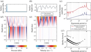
We explore two general sources here. First we model an impulsive force on the free surface at the top of the conduit by setting the right-hand side of the top pressure boundary condition (2.51) equal to
 $\mathscr{I}(t)$
(with units of Pa). We also consider an internal volumetric source, as might arise from volumetric transformation strain or injection of mass, by setting the right-hand side of (2.41) equal to
 $\dot{\mathscr{M}}(z,t)$
(with units of
 $1~\text{s}^{-1}$
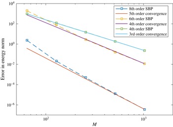
). The equations are spatially discretized as before, but are now solved in the time domain using an explicit Runge–Kutta method for time stepping. See appendix A for details of the method and appendix B for convergence tests verifying stability and high-order accuracy.
In the following, we assume Gaussian sources,
 $$\begin{eqnarray}\displaystyle & \displaystyle \dot{\mathscr{M}}(z,t)=F_{M}\exp \left[-\frac{(t-t_{FM})^{2}}{2{\it\sigma}_{FM}^{2}}\right]\exp \left[-\frac{(z-z_{FM})^{2}}{2{\it\sigma}_{Z}^{2}}\right]\!, & \displaystyle\end{eqnarray}$$
 $$\begin{eqnarray}\displaystyle & \displaystyle \mathscr{I}(t)=F_{I}\exp \left[-\frac{(t-t_{FI})^{2}}{2{\it\sigma}_{FI}^{2}}\right]\!, & \displaystyle\end{eqnarray}$$
with
 $F_{M}$
,
 $F_{I}$
the source amplitudes,
 $t_{FM}$
,
 $z_{FM}$
,
 $t_{FI}$
the time and spatial location of source excitations, and
 ${\it\sigma}_{FI}$
,
 ${\it\sigma}_{FM}$
,
 ${\it\sigma}_{Z}$
the duration and spatial width of the sources.
5.1 Connection to conduit eigenmodes and to observables
Before we present numerical solutions, we point out that time-dependent solutions to the inhomogeneous equations do not directly provide information about which of the conduit eigenmodes from (4.1) are excited. Neither do they reveal how excitation of waves within the conduit relates to potential observations. There is, however, a formal procedure for connecting these two calculations. We first Laplace transform the semi-discrete, inhomogeneous governing equations (A 2)–(A 5), yielding a linear system of the form
 $$\begin{eqnarray}s\tilde{\boldsymbol{u}}=\unicode[STIX]{x1D63D}\tilde{\boldsymbol{u}}+\boldsymbol{b}_{FI}\tilde{f}_{FI}(s)+\boldsymbol{b}_{FM}\tilde{f}_{FM}(s),\end{eqnarray}$$
where
 $\tilde{\boldsymbol{u}}$
and
 $\unicode[STIX]{x1D63D}$
are defined as before, and the two terms of the form
 $\boldsymbol{b}\tilde{f}(s)$
are the Laplace-transformed source vectors associated with surface impulses (subscript
 $FI$
) and internal volumetric or mass sources (subscript
 $FM$
). We have assumed a source process that permits us to factor the source into a vector
 $\boldsymbol{b}$
capturing the spatial dependence of the source and another function,
 $f(t)$
, carrying the source time dependence and magnitude. For this special case
 $\boldsymbol{b}$
is independent of Laplace parameter
 $s$
. Discussion of
 $\boldsymbol{b}$
and
 $f$
is presented in appendix A.
 $\unicode[STIX]{x1D63D}$
can be decomposed as
 $\unicode[STIX]{x1D63D}=\unicode[STIX]{x1D652}{\it\bf\Lambda}\unicode[STIX]{x1D652}^{-1}$
, with
 $\unicode[STIX]{x1D652}$
a matrix containing the eigenvectors of
 $\unicode[STIX]{x1D63D}$
as columns and
 ${\it\bf\Lambda}=\text{diag}({\it\lambda}_{1},\ldots ,{\it\lambda}_{3(M+2)+1})$
a diagonal matrix of eigenvalues
 ${\it\lambda}_{i}$
(denoted as
 $s$
in the previous section on the eigenvalue problem). As mentioned in § 3,
 $\unicode[STIX]{x1D63D}$
is non-normal, so although
 $\unicode[STIX]{x1D63D}$
is diagonalizable, eigenfunctions are not necessarily orthogonal (
 $\unicode[STIX]{x1D652}$
is not unitary). We have experimented with partially symmetrizing the eigenproblem by rescaling
 $\boldsymbol{u}(t)$
such that its
 $L_{2}$
norm is the total mechanical energy density, which greatly reduces the condition number of the resulting coefficient matrix and improves numerical accuracy. However, all calculations have shown that the longest-period modes are nearly orthogonal and we will show that we can accurately recover the time-domain solution with the method described below. This suggests that our problem is not far from normal, at least for the range of parameters we have studied thus far.
Suppose we are interested in a particular set of observations
 $\boldsymbol{y}(t)$
, which are a linear functional of the fields
 $\boldsymbol{u}(t)$
. Examples of observations include the ground displacements in an elastic half-space caused by pressure changes applied to the surface of the conduit, motions of the lava lake surface, and infrasound signals generated by oscillations of the lava lake surface. From linearity it follows that there exists an observation matrix linking the observables to the fields within the conduit, expressed in the Laplace domain as
 $$\begin{eqnarray}\tilde{\boldsymbol{y}}=\mathscr{C}\tilde{\boldsymbol{u}}.\end{eqnarray}$$
In general
 $\mathscr{C}=\mathscr{C}(s)$
(such that the observation at time
 $t$
depends on the fields at all times leading up to
 $t$
), but in this study we restrict attention to observables for which
 $\mathscr{C}$
is independent of
 $s$
.
Using (5.3) the solution of (5.4) is then
 $$\begin{eqnarray}\tilde{\boldsymbol{y}}=\mathscr{H}_{FI}\tilde{f}_{FI}+\mathscr{H}_{FM}\tilde{f}_{FM},\end{eqnarray}$$
where
 $\mathscr{H}_{FI}(s)$
and
 $\mathscr{H}_{FM}(s)$
are transfer functions between the observables and surface impulse and internal volumetric/mass sources, respectively, which take the form
 $$\begin{eqnarray}\mathscr{H}(s)=\mathscr{C}\unicode[STIX]{x1D652}\text{diag}\left(\frac{1}{s-{\it\lambda}_{1}},\ldots ,\frac{1}{s-{\it\lambda}_{3(M+2)+1}}\right)\unicode[STIX]{x1D652}^{-1}\boldsymbol{b}.\end{eqnarray}$$
Excitation of waves by a Gaussian pressure impulse on the otherwise traction-free upper boundary. Source is centred at 10 s, with amplitude 10 kPa and duration half-width 1 s.
 ${\it\tau}=1$
s and
 $n_{t}=0.01$
. (a) Pressure at free surface and (b) height of free surface as a function of time. (c) Excitation amplitude of free surface eigenmodes from the transfer function of
 $h$
(5.6) for the free surface height (blue line) and pressure at exsolution (red line). (d) Pressure perturbation and (e) velocity perturbation within the conduit. Dashed line is exsolution depth. (f) Quality factor
 $Q$
of conduit eigenmodes (figure 6) as a function of mode period. Panels (c) and (f) together express which modes are excited and which will contribute to some particular observable field. A mode can be excited but not expressed in some field.

The time-domain solution may be recovered by inverting the Laplace transform through use of the residue theorem, or alternatively by approximating the integral as a discrete inverse Fourier transform (e.g. Davies & Martin Reference Davies and Martin1979). We find that numerically the latter is the more accurate method. This method requires that the time series is chosen to be long enough that the least damped mode decays sufficiently to prevent wrap-around effects in the source excitation, and thus is not an efficient method in general. However, we can accurately reproduce the time evolution calculated by the time-domain method for a single or multiple observables.
5.2 Source excitation by top boundary pressure forcing
We first study the problem of a pressure impulse on the upper boundary of an initially static magma column. This could arise from perturbations to the surface of a lava lake by, for example, rockfall or shallow near-surface degassing bursts. Figure 8 illustrates results from a test case using
 $L=3$
km,
 ${\it\tau}=1$
s, and
 $n_{t}=0.01$
, with source pressure amplitude
 $F_{I}=10$
kPa centred in time at
 $t_{FI}=10$
s after the start of the simulation, with duration
 ${\it\sigma}_{FI}=1$
s. This pressure pulse initially pushes the free surface down (figure 8
b), generating a downward-propagating wave carrying a pressure increase and downward velocity perturbation. At the exsolution depth (
 $z\approx 1420$
m) this wave is partially reflected. The transmitted wave continues into the single-phase region at depth, where it excites high-frequency oscillations. The reflected wave causes low-frequency oscillations in the upper, bubbly region. Damping in these simulations is only through energy lost by non-equilibrium BGR, as we have assumed inviscid magma. Inclusion of viscosity would result in smaller free surface height variations and more rapid decay of oscillations.
We then use the transfer function in (5.6) to obtain excitation amplitudes of individual eigenmodes. Figure 8(c) shows the magnitude of
 $\mathscr{H}_{FI}(s)$
as a function of excitation period (
 $2{\rm\pi}/\text{Im}(s)$
with purely imaginary
 $s$
), for two choices of
 $y$
: the free surface height
 $h$
and the pressure perturbation at the exsolution depth
 $p_{\mathit{exsolve}}$
. The latter is a crude proxy for excitation of seismic waves and ground displacements by pressure perturbations on the conduit walls. The former is inverted to the time domain to demonstrate that the Fourier transform inversion method reproduces finite difference calculations accurately and is plotted on top of the time-dependent solution in figure 8(b). Figure 8(f) then shows the period and quality factor of eigenmodes obtained during study of the homogeneous problem. Comparison to figure 8(c) shows that the top forcing excites long-period modes at much larger amplitude than short-period modes, as observed in the time-dependent simulations.
5.3 Source excitation by an impulsive internal mass source
The second type of source we study is an impulsive, localized volumetric source within the conduit. This could arise from influx or outflux of mass from a branching sill or dike, or any other discrete dilational event. We explore a case where dilation rate is
 $F_{M}=0.05$
1 s
 $^{-1}$
, with
 $t_{FM}=10$
s,
 ${\it\sigma}_{FM}=1$
s, and spatial half-width
 ${\it\sigma}_{Z}=10$
m, all other parameters as in the top forcing example of § 5.2. Figure 9 shows two examples, one where the volumetric source is below exsolution (
 $z_{FM}=2$
km, figure 9
a) and one where the source is above exsolution (
 $z_{FM}=1$
km, figure 9
b).
(a,c,e) Excitation of waves by an internal mass source, a Gaussian source with spatial extent
 ${\it\sigma}_{Z}=10$
m, temporal duration
 ${\it\sigma}_{FM}=1$
s, injected at
 $z_{FM}=2$
km depth (below exsolution) at time
 $t_{FM}=10$
s. (a) is free surface height, (c) is pressure perturbation amplitude in kPa versus time. (e) is transfer function amplitude of pressure at the exsolution depth and surface height versus mode period in seconds. (b,d,f) Same as part (a,c,e), except the mass source is injected at
 $z_{FM}=1$
km depth (above exsolution).

Looking first at the amplitude of the pressure perturbations, we see that sources below exsolution generate much higher pressures than sources above exsolution. This can be understood in terms of the difference in fluid properties between bubbly and non-bubbly magma: the fluid bulk modulus is
 ${\sim}$
4 orders of magnitude larger at 2 km depth than at 1 km depth. From the amplitude of pressure eigenmode excitation in figure 9(e,f) (amplitude of transfer function
 $\mathscr{H}_{FM}(s)$
for pressure at the exsolution depth) we also see that high-frequency modes are excited in the single-phase region when the source is below the exsolution depth, but not when the source is above it. By the time perturbations reach the free surface, however, in both cases the high-frequency modes have been damped out, and the free surface height still primarily records long-period modes from the bubbly upper conduit.
5.4 Influence of bottom boundary condition
All results so far assume a constant-pressure bottom boundary condition, so fluid can flow freely in and out of the conduit from some deeper magma reservoir or chamber. This is not the only possible boundary condition for real volcanic systems. Another possibility is a no-flow (zero-velocity) boundary condition, which would lead to variations in pressure during oscillatory motion of the magma column. We can assess the conditions under which either of these boundary conditions is realistic in the context of a simple model of the reservoir that is coupled to the bottom boundary of the conduit. We assume uniform pressure throughout the reservoir, which might be a chamber or sill within an elastic solid.
We combine a statement of mass balance for the reservoir, neglecting influx from below, with linearized expressions relating changes in fluid density and reservoir volume to pressure changes (Segall Reference Segall2010). This reservoir model is coupled to the conduit by setting reservoir pressure equal to the pressure at the bottom of the conduit,
 $P_{b}$
, and setting volume flux out of the reservoir into the conduit equal to
 $A(0)V_{b}$
, where
 $A(0)$
is the cross-sectional area at the bottom of the conduit and
 $V_{b}$
is the velocity there. The result is an ordinary differential equation linking
 $P_{b}$
and
 $V_{b}$
:
 $$\begin{eqnarray}\frac{\text{d}P_{b}}{\text{d}t}=-{\it\epsilon}_{r}V_{b},\end{eqnarray}$$
where
 ${\it\epsilon}_{r}=A(0)/{\it\beta}_{r}V_{r}$
contains the overall compressibility
 ${\it\beta}_{r}$
(the sum of chamber or sill compressibility and fluid compressibility) and the reservoir volume
 $V_{r}$
. We have assumed for simplicity that the conduit and chamber have the same bubble content.
Fourier transforming in time, with angular frequency
 ${\it\omega}$
, permits us to define the impedance of the reservoir system as the ratio of the Fourier-transformed pressure and velocity:
 $$\begin{eqnarray}\frac{\tilde{P}_{b}}{\tilde{V}_{b}}=-\frac{{\it\epsilon}_{r}}{\text{i}{\it\omega}}.\end{eqnarray}$$
We then compare this impedance to the impedance of a wave in the conduit,
 ${\it\rho}_{b}C_{b}$
, where
 ${\it\rho}_{b}$
and
 $C_{b}$
are the density and phase velocity of the wave at the bottom of the conduit. The impedance ratio,
 $$\begin{eqnarray}{\it\Gamma}=-\frac{{\it\epsilon}_{r}}{\text{i}{\it\omega}{\it\rho}_{b}C_{b}},\end{eqnarray}$$
determines how waves reflect from the reservoir (e.g. Lighthill Reference Lighthill1978). When
 ${\it\Gamma}\ll 1$
, then
 $P_{b}\approx \text{constant}$
; when
 ${\it\Gamma}\gg 1$
, then
 $V_{b}\approx 0$
.
We consider two examples of reservoir systems to estimate the impedance ratio. First, assume the conduit, of radius
 ${\sim}$
10 m, is connected to a magma-filled sill of radius
 ${\sim}$
1 km and thickness
 ${\sim}$
1 m. Compressibility of the system is principally from opening/closing the sill, such that
 ${\it\beta}_{r}$
is approximately equal to the overpressure
 ${\sim}$
10 MPa in the sill (i.e. the difference between magma pressure and compressive normal stress acting to close the sill). We also take
 ${\it\rho}_{b}C_{b}\sim 10^{6}$
Pa s m
 $^{-1}$
. Thus,
 ${\it\epsilon}_{r}\sim 10^{3}$
Pa m
 $^{-1}$
. It follows that at periods less than
 ${\sim}$
1000 s the constant-pressure condition is appropriate.
As a second example, we assume the reservoir is a spherical magma chamber of radius
 ${\sim}$
100 m; we again take the conduit radius to be
 ${\sim}$
10 m. Furthermore,
 ${\it\beta}_{r}$
is approximately equal to the reciprocal of the magma bulk modulus (
 ${\sim}$
10 GPa), with a slight correction due to the elastic compliance of the chamber. In this case,
 ${\it\epsilon}_{r}\sim 10^{6}$
Pa m
 $^{-1}$
, and here for modes with periods longer than
 ${\sim}$
10 s, the no-flow boundary condition is appropriate.
The major difference between the constant-pressure and no-flow bottom boundary conditions lies in the longest-period eigenmode. For the constant-pressure boundary condition, this longest period has the majority of kinetic energy residing in the bubble-free region (figure 7). Thus, it represents oscillatory mass transport in and out of the conduit. For the no-flow boundary condition, this mode is absent, and the longest-period mode is one that resides in the bubbly region (figure 10 a, dashed curve).
(a) Magnitude of transfer function between top pressure forcing and pressure at the exsolution depth, varying total conduit length
 $L$
, comparing constant-pressure (solid) and zero-velocity (dashed) bottom boundary conditions.
 $n_{t}=0.01$
and
 ${\it\tau}=1$
s. Note that modes localized above exsolution are not sensitive to
 $L$
or bottom boundary condition. (b) Same as panel (a) (and with
 $p=0$
bottom boundary condition), but varying total volatile content with
 $L=3$
km. We also include a case of joint H
 $_{2}$
O and CO
 $_{2}$
solubility (Papale, Moretti & Barbato Reference Papale, Moretti and Barbato2006) that represents typical volatile contents at Kilauea, HI. Inset shows depth variation of gas mass fraction in the base state.

5.5 Influence of conduit length, total volatile content, and solubility law
We next briefly explore how mode properties and excitation (the latter expressed via transfer functions) are influenced by the conduit length, total volatile content, and solubility law.
One might reasonably speculate that the longest eigenmode periods are simply set by the conduit length
 $L$
, as they are in organ pipes containing a homogeneous fluid. Figure 10 explores this in more detail for the
 $p=0$
bottom boundary condition, using the top boundary pressure excitation and transfer function for the pressure at the exsolution depth to probe the sensitivity of mode properties to
 $L$
. As we increase
 $L$
, some of the modes vary systematically. The fundamental mode (Ex 1) shifts to longer periods as
 $L$
increases (figure 10
a), consistent with an increase in effective mass (due to the increase of the length of the liquid melt region), with the restoring force from magma compression immediately above the exsolution depth relatively unaltered. Similarly, the shorter-period modes in family II (such as Ex 3, with
 ${\sim}$
1 s period) that are localized within the liquid melt region at depth shift to larger periods as
 $L$
increases. In contrast, modes with periods between
 ${\sim}$
10 and 50 s that are oscillations within the bubbly region (modes in family I such as Ex 2) are largely insensitive to
 $L$
, since it is the length of the bubbly magma region (set by total volatile content
 $n_{t}$
) that influences their period.
Finally, switching from a
 $p=0$
to
 $v=0$
bottom boundary condition eliminates flow in and out of the conduit, and the fundamental mode no longer exists. Modes such as Ex 2 are effectively unaltered (and they are insensitive to
 $L$
), while those such as Ex 3 have longer periods (close to double those for
 $p=0$
) that reflect the changed boundary conditions (figure 10
a).
We next explore, for fixed
 $L$
, the influence of the total volatile content
 $n_{t}$
, and hence the length of the bubbly magma region, on mode properties (figure 10
b). Modes of all periods are sensitive to the total volatile content
 $n_{t}$
, but in differing ways, as illustrated by comparison of the red and blue curves in figure 10(b), corresponding to
 $n_{t}=0.005$
and 0.01, respectively. The period of the fundamental open-ended pipe mode (Ex 1) decreases as
 $n_{t}$
increases, because the mass (of the liquid melt region at depth) decreases as the exsolution surface moves to greater depths. In contrast, the periods of the long-period modes such as Ex 2 increase as
 $n_{t}$
increases. These modes reside within the bubbly magma above the exsolution depth, and the extent of this region increases with
 $n_{t}$
.
Of course, real magmas have a more complicated volatile content, with H
 $_{2}$
O as well as lesser amounts of CO
 $_{2}$
and SO
 $_{2}$
(as well as other volatiles) that have much lower solubilities. Although a detailed exploration of the consequences of more complex solubility laws is outside the scope of this paper, we include in figure 10(b) a calculation using the joint H
 $_{2}$
O and CO
 $_{2}$
solubility model of Papale et al. (Reference Papale, Moretti and Barbato2006) as the gas base state. Using volatile contents typical of shallowly stored Kilauea magmas (Gerlach & Graeber Reference Gerlach and Graeber1985) as a guide, we use a H
 $_{2}$
O mass fraction of
 $n_{t,w}=0.006$
and a CO
 $_{2}$
mass fraction of
 $n_{t,c}=4\times 10^{-4}$
. The inset demonstrates that the background gas profile exhibits a more gradual decline with depth than the case of pure water, due to the persistence of CO
 $_{2}$
bubbles at depths greater than that at which all H
 $_{2}$
O bubbles have dissolved. Nevertheless, this case still exhibits a large contrast in properties at the water exsolution depth. Such a result is not unexpected, since water is more than an order of magnitude more abundant that CO
 $_{2}$
in this example (a result that holds generally for magmas). Therefore the segmentation of conduit eigenmodes by water exsolution should be even more pronounced for magmas that contain greater total volatile contents, such as at subduction zones, where H
 $_{2}$
O may reach 6–8 % by mass and CO
 $_{2}$
up to 0.3 % (Wallace Reference Wallace2005).
6 Discussion
We have developed a linear theory for the resonant modes of a column of bubbly magma in a volcanic conduit. Stratification (depth dependence of fluid properties in the base state) and non-equilibrium BGR are important controls on the spatial structure, periods, and damping rates of these eigenmodes. We connected eigenmodes to source excitation in the time domain with two numerical methods, a transfer function approach that utilizes conduit eigenfunctions, and direct finite difference solution of the governing equations. The source type, and depth in the case of internal sources, determine which eigenmodes are excited.
We have chosen the simplest possible background state of a magma column at rest in mechanical and thermodynamic equilibrium. The systems most closely matching this idealization are open-vent volcanoes with active lava lakes such as Halema’uma’u (Kilauea, HI) and Erebus (Antarctica), though additional processes (discussed below) might need to be added to our initial model to properly characterize these systems. As mentioned in the introduction, impulsive disturbances such as rockfall into the open vent or bursting of gas slugs trigger VLP seismic signals (tens of seconds, Aster et al. Reference Aster, Mah, Kyle, McIntosh, Dunbar, Johnson, Rulz and McNamara2003; Chouet & Dawson Reference Chouet and Dawson2013) that ring down over several minutes, quite similar to the longest-period eigenmodes we have identified in our study.
Future application of this model to VLP seismicity will benefit from further model development, specifically inclusion of viscous drag, degassing (relative motion of gas and liquid phases), and branching cracks (dikes and sills) at depth. Both Halema’uma’u and Erebus involve low-viscosity magmas, and as discussed in § 1, treatment of drag from viscous boundary layers (e.g. Lipovsky & Dunham Reference Lipovsky and Dunham2015) is needed for mode periods less than
 ${\sim}$
100 s. This necessitates resolution of radial variations in the velocity field. Both Kilauea and Erebus also exhibit slow, background convection, with bubbles rising buoyantly relative to the liquid melt and denser (degassed) magma sinking. This convection and associated gas loss through the surface, once cross-sectionally averaged, would increase density, bulk modulus, and sound speed in the upper part of the conduit relative to the magmastatic model (§ 2.4). Indeed, inferred values of density in the Kilauea lava lake from continuous gravity (Carbone et al.
Reference Carbone, Poland, Patrick and Orr2013) and direct measurement of near-surface samples (Eychenne et al.
Reference Eychenne, Houghton, Swanson, Carey and Swavely2015) are in the range 400–1000 kg m
 $^{-}3$
.
Finally, there is evidence that the conduit beneath the lava lake at Kilauea connects to one or more cracks at depth. For example, seismic waveform modelling suggests coupling between oscillatory motion of the magma column and the solid Earth occurs in a set of dikes at approximately 1 km depth (Chouet & Dawson Reference Chouet and Dawson2011, Reference Chouet and Dawson2013; Dawson & Chouet Reference Dawson and Chouet2014). Ground deformation inversions place a magma reservoir at similar depths (e.g. Poland, Miklius & Montgomery-Brown Reference Poland, Miklius, Montgomery-Brown, Poland, Takahashi and Landowski2014). This motivates the introduction of a crack into our model, which will influence mode properties. For a crack at the base of the conduit, responding at relatively long time scales compared to the time of crack wave propagation across the crack, it might be possible to idealize the crack using the boundary condition introduced in (5.7). Adding one or more branching cracks, and studying their influence on mode properties and seismic expression of the modes, is a logical next step.
At the top of the conduit, coupling of magmatic fluid motions to an overlying stratified atmosphere may occur, producing infrasonic waves (e.g. Garcés & McNutt Reference Garcés and McNutt1997). We can still use the transfer function approach to infer mode excitation in these cases, if we have the appropriate model for atmospheric acoustic-gravity wave propagation that can serve to form the observation matrix, and the coupling between the conduit and atmosphere is linear.
Better constraints on non-equilibrium BGR are also warranted. The time scale
 ${\it\tau}$
for non-equilibrium BGR is not well known in magmas. It could reasonably lie in the range
 ${\sim}$
1–100 s, based on typical bubble sizes and diffusivity of water and CO
 $_{2}$
in silicate melts, and available experimental results on natural silica-rich samples (e.g. Watkins, Manga & DePaolo Reference Watkins, Manga and DePaolo2012). We have shown that the periods and spatial structure of conduit eigenmodes are affected by
 ${\it\tau}$
(figure 6), with the largest damping for periods of approximately
 ${\it\tau}$
(i.e.
 ${\it\sigma}/2{\rm\pi}\sim 1$
, figure 4). Observations of oscillations at open-vent systems such as Kilauea, with periods in the
 ${\sim}$
30 s range (e.g. Chouet & Dawson Reference Chouet and Dawson2013), suggest that either
 ${\it\tau}$
is much larger or smaller than this period, or that energy dissipation from non-equilibrium BGR is smaller than our models suggest (e.g. due to smaller differences between non-equilibrium and equilibrium properties). Finally,
 ${\it\tau}$
will undoubtedly vary as a function of depth in real conduits, in response to depth variations in bubble size and spacing, and variable volatile species present. We reserve exploration of this effect for future work.
Despite the need to introduce additional complexity into our models, this initial study suggests several exciting opportunities. Perhaps the most important result to emerge is the sensitivity of the longest-period eigenmodes to total magmatic volatile content and to the solubility law used in the modelling (figure 10 b). Observations of VLP seismicity might thus be used to monitor variations in volatile content over time. Total volatile content is one of the most important factors governing volcanic eruption style (e.g. effusive or explosive), and can vary widely over the course of a single eruptive episode and between volcanoes. Total volatile contents currently are inferred primarily from melt inclusions that must be gathered after eruptive activity is over (e.g. Métrich & Wallace Reference Métrich and Wallace2008). In addition, with independent constraints on total volatile content from petrology and melt inclusions, modelling of VLP seismicity might be used for in situ validation of experimentally determined solubility laws and non-equilibrium mass exchange in bubbly magmas.
Acknowledgements
This work was supported by the National Science Foundation (EAR-1143623 to L.K., EAR-1114073 to E.M.D.) and the Alfred P. Sloan Foundation (BR2012-097 to E.M.D.). We thank O. O’Reilly and B. A. Erickson for discussions and advice on mathematical and numerical issues, and the three anonymous reviewers for their extremely useful suggestions.
Appendix A. Discrete governing equations
In this appendix we present a finite difference method for solving the continuous governing equations (2.40)–(2.42) and (2.49) and boundary conditions (2.50) and (2.51). The coefficients of the equations are discontinuous across the exsolution surface, making it advantageous to divide the domain into two subdomains, one on either side of the exsolution surface. Solutions in these two subdomains are coupled by appropriate interface conditions across the exsolution surface. All calculations in this study utilize this split domain method, and we provide details on the interface coupling below. However, for simplicity, we begin by presenting the numerical method for a single domain.
Spanning the domain
 $0\leqslant z\leqslant L$
is a set of
 $N+1$
, possibly non-uniformly spaced, grid points
 $z_{i}$
,
 $i=0,\ldots ,N$
. A field such as
 $v(z,t)$
is approximated at the grid points, with the grid values stored in a vector
 $\boldsymbol{v}(t)$
having components
 $v_{i}(t)\approx v(z_{i},t)$
. Spatial differences are approximated with a summation-by-parts (SBP) differentiation matrix
 $\unicode[STIX]{x1D63F}$
, such that the vector
 $\unicode[STIX]{x1D63F}\boldsymbol{v}$
contains approximations to
 $\partial v/\partial z$
at the grid points. SBP operators take the form
 $$\begin{eqnarray}\unicode[STIX]{x1D63F}=\unicode[STIX]{x1D643}^{-1}\unicode[STIX]{x1D64C},\end{eqnarray}$$
where
 $\unicode[STIX]{x1D643}$
is a symmetric positive definite matrix (diagonal in this work) and
 $\unicode[STIX]{x1D64C}$
is an almost skew symmetric matrix with the property that
 $\unicode[STIX]{x1D64C}^{\text{T}}+\unicode[STIX]{x1D64C}=\text{diag}[-1~0~\ldots ~0~1]$
(Kreiss & Scherer Reference Kreiss, Scherer and de Boor1974, Reference Kreiss and Scherer1977; Strand Reference Strand1994; Gustafsson et al.
Reference Gustafsson, Kreiss and Oliger1995).
Boundary conditions are imposed by including penalty terms in the semi-discrete governing equations, called simultaneous approximation terms (SAT) (Carpenter et al.
Reference Carpenter, Gottlieb and Abarbanel1994). The number of boundary conditions and which equations must be penalized are determined through the characteristics of this hyperbolic set of equations. The characteristic variables associated with waves propagating in the
 $+z$
and
 $-z$
directions are
 $p+Zv$
and
 $p-Zv$
, respectively, where we have introduced the acoustic impedance
 $Z=\bar{{\it\rho}}C$
for notational simplicity. Therefore, we must place one boundary condition on
 $p+Zv$
at
 $z=0$
and one boundary condition on
 $p-Zv$
at
 $z=L$
. These boundary conditions can involve the other characteristic variable, of course, which carries information from within the domain to its boundaries.
The semi-discrete equations are
 $$\begin{eqnarray}\displaystyle & \displaystyle \frac{\text{d}\boldsymbol{v}}{\text{d}t}=-\frac{1}{\bar{{\it\rho}}}\unicode[STIX]{x1D643}^{-1}\unicode[STIX]{x1D64C}\,\boldsymbol{p}-\frac{g}{K}\boldsymbol{p}+ga\boldsymbol{n}-{\it\theta}_{1}(v_{0}-\hat{v}_{0})\boldsymbol{e}_{0}-{\it\theta}_{2}(v_{N}-\hat{v}_{N})\boldsymbol{e}_{N}, & \displaystyle\end{eqnarray}$$
 $$\begin{eqnarray}\displaystyle & \displaystyle \frac{\text{d}\,\boldsymbol{p}}{\text{d}t}=-\frac{K}{A}\unicode[STIX]{x1D643}^{-1}\unicode[STIX]{x1D64C}A\boldsymbol{v}+\bar{{\it\rho}}g\boldsymbol{v}-\frac{aK}{{\it\tau}}(\boldsymbol{n}+b\boldsymbol{p})-{\it\theta}_{3}(p_{0}-\hat{p}_{0})\boldsymbol{e}_{0}-{\it\theta}_{4}(p_{N}-\hat{p}_{N})\boldsymbol{e}_{N}, & \displaystyle\end{eqnarray}$$
 $$\begin{eqnarray}\displaystyle & \displaystyle \frac{\text{d}\boldsymbol{n}}{\text{d}t}=-\bar{{\it\rho}}gb\boldsymbol{v}-\frac{1}{{\it\tau}}(\boldsymbol{n}+b\boldsymbol{p}), & \displaystyle\end{eqnarray}$$
 $$\begin{eqnarray}\displaystyle & \displaystyle \frac{\text{d}h}{\text{d}t}=\hat{v}_{N}, & \displaystyle\end{eqnarray}$$
where
 $\boldsymbol{e}_{0}=[1~0~\cdots ~0]^{\text{T}}$
and
 $\boldsymbol{e}_{N}=[0~\cdots ~0~1]^{\text{T}}$
are vectors that isolate the penalty terms to the boundary points. Coefficients not in bold type are now diagonal matrices containing possibly spatially variable properties such as
 $\bar{{\it\rho}}$
,
 $A$
, etc., with
 $1/\bar{{\it\rho}}$
really being the inverse of the diagonal matrix
 $\bar{{\it\rho}}$
. Scalars
 ${\it\theta}_{1}{-}{\it\theta}_{4}$
are penalty parameters chosen to ensure a stable numerical discretization, while hatted variables
 $\hat{v}_{0},\hat{v}_{N},\hat{p}_{0},\hat{p}_{N}$
are target values for velocity and pressure at the boundary points. These are chosen to satisfy the desired boundary conditions exactly,
 $$\begin{eqnarray}\hat{p}_{0}=0\quad \text{and}\quad \hat{p}_{N}=\bar{{\it\rho}}gh,\end{eqnarray}$$
while preserving the characteristic variable carrying information from the interior of the domain to the boundary,
 $$\begin{eqnarray}p_{0}-Z_{0}v_{0}=\hat{p}_{0}-Z_{0}\hat{v}_{0}\quad \text{and}\quad p_{N}+Z_{N}v_{N}=\hat{p}_{N}+Z_{N}\hat{v}_{N}.\end{eqnarray}$$
It follows that
 $$\begin{eqnarray}\hat{v}_{0}=v_{0}-\frac{p_{0}}{Z_{0}}\quad \text{and}\quad \hat{v}_{N}=v_{N}+\frac{p_{N}-\bar{{\it\rho}}_{N}gh}{Z_{N}}.\end{eqnarray}$$
Following Kozdon, Dunham & Nordstrom (Reference Kozdon, Dunham and Nordstrom2011), we find that
 $$\begin{eqnarray}{\it\theta}_{1}={\it\theta}_{3}=C/H_{00},\quad {\it\theta}_{2}={\it\theta}_{4}=C/H_{NN}\end{eqnarray}$$
ensures stability, as shown below.
When adding sources to the semi-discrete equations (A 2)–(A 5), we decompose pressure and volumetric contributions in (5.1) and (5.2) into a vector
 $\boldsymbol{b}$
that contains the spatial dependence and a function
 $f(t)$
that contains time dependence and magnitude. In the context of (5.3), the
 $\boldsymbol{b}$
vectors (length
 $3(M+2)+1$
) take the form
 $$\begin{eqnarray}\boldsymbol{b}_{FM}=[\mathbf{0}~~b_{FM}(\boldsymbol{z})~~\mathbf{0}~~0]^{\text{T}},\end{eqnarray}$$
where
 $b_{FM}(z)=K(z)\exp (-0.5(z-z_{FM})^{2}/(2{\it\sigma}_{Z}^{2}))$
and
 $\mathbf{0}$
is a
 $M+2$
length vector of zeros, while
 $\boldsymbol{b}_{FI}$
contains corrections to the surface penalty terms but is otherwise zero. The
 $f$
are specified in (5.1), without the dimensionless spatial exponential, and (5.2), and thus have units given by
 $F_{M}$
and
 $F_{I}$
, respectively.
One of the principal benefits for using SBP–SAT is the ease with which we can prove stability of the method, done by constructing a discrete energy balance. Before doing this we note that the SBP operator is analogous to integration by parts. For example, if
 $$\begin{eqnarray}(u,v)=\int _{0}^{L}u(z)v(z)\,\text{d}z\quad \text{and}\quad (\boldsymbol{u},\boldsymbol{v})_{h}=\boldsymbol{u}^{\text{T}}\unicode[STIX]{x1D643}\boldsymbol{v}\end{eqnarray}$$
are continuous and discrete inner products, respectively, then
 $$\begin{eqnarray}\left(p,\frac{\text{d}p}{\text{d}z}\right)=\frac{1}{2}(p(L)^{2}-p(0)^{2})\quad \text{and}\quad (\boldsymbol{p},\unicode[STIX]{x1D643}^{-1}\unicode[STIX]{x1D64C}\,\boldsymbol{p})_{h}=\frac{1}{2}(p_{N}^{2}-p_{0}^{2}).\end{eqnarray}$$
To construct a discrete energy balance we multiply (A 2) by
 $\boldsymbol{v}^{\text{T}}\unicode[STIX]{x1D643}A$
, (A 3) by
 $\boldsymbol{p}^{\text{T}}\unicode[STIX]{x1D643}A$
, (A 4) by
 $\boldsymbol{n}^{\text{T}}\unicode[STIX]{x1D643}A$
, and (A 5) by
 $\bar{{\it\rho}}_{N}gA_{N}h$
, and then sum. Doing the same to the transpose of (A 2)–(A 5), adding the results, and dividing by two, we arrive at
 $$\begin{eqnarray}\frac{\text{d}E_{h}}{\text{d}t}=-\frac{A_{0}}{Z_{0}}p_{0}^{2}-\frac{A_{N}}{Z_{N}}(p_{N}-\bar{{\it\rho}}_{N}gh)^{2}-(\boldsymbol{n}+b\boldsymbol{p})^{\text{T}}\unicode[STIX]{x1D643}A\frac{a}{b{\it\tau}}(\boldsymbol{n}+b\boldsymbol{p}),\end{eqnarray}$$
where the discrete energy
 $E_{h}$
is defined as
 $$\begin{eqnarray}E_{h}=\frac{1}{2}\boldsymbol{v}^{\text{T}}\unicode[STIX]{x1D643}A\bar{{\it\rho}}\boldsymbol{v}+\frac{1}{2}\boldsymbol{p}^{\text{T}}\unicode[STIX]{x1D643}\frac{A}{K}\boldsymbol{p}+\frac{1}{2}\boldsymbol{n}^{\text{T}}\unicode[STIX]{x1D643}\frac{aA}{b}\boldsymbol{n}+\frac{1}{2}\bar{{\it\rho}}_{N}gA_{N}h^{2}.\end{eqnarray}$$
Comparison to the continuous energy balance in (2.52) and (2.53) shows a correspondence to each term in the discrete version, except for the first two terms on the right-hand side of (A 13). Those terms, which vanish when the boundary conditions (2.50) and (2.51) are exactly satisfied, correspond to a slight amount of numerical dissipation that vanishes with mesh refinement.
The discrete energy
 $E_{h}$
is thus a strictly decreasing function, and our numerical method is stable. Our method uses SBP operators that have interior accuracy
 $q$
and boundary accuracy
 $r=q/2$
, leading to a global accuracy of
 $p=r+1$
(Gustafsson Reference Gustafsson1975). As discussed in the next section we generally use SBP operators with
 $q=8$
(Mattsson, Almquist & Carpenter Reference Mattsson, Almquist and Carpenter2014). Time stepping is done with a fourth-order-accurate low-storage Runge–Kutta method (Carpenter & Kennedy Reference Carpenter and Kennedy1996).
The numerical method presented above can be generalized by dividing the domain into two or more subdomains. Each subdomain is separately discretized and the solutions in adjacent subdomains are coupled via interface conditions (SAT penalties). For our problem, we divide the domain across the exsolution surface. Interface conditions are continuity of mass flux
 $\bar{{\it\rho}}Av$
and pressure
 $p$
. In this case, the energy balance contains additional numerical dissipation terms that vanish with mesh refinement. Dividing the domain in this manner substantially increases the accuracy of the numerical solution. For later reference, we refer to the total number of points in both subdomains as
 $M+2$
.
Appendix B. Convergence of the numerical solution
We demonstrate convergence of the numerical method developed in § 4 at the expected order of accuracy via the method of manufactured solutions (Roache Reference Roache1998). This method involves constructing an analytic solution to the governing equations (2.40)–(2.42) and (2.49) by stipulating an arbitrary set of pressure, velocity, and gas mass fraction functions, then imposing source terms and boundary data such that these functions are satisfied by the governing equations. We choose functions that test all relevant aspects of the governing equations: time dependence, spatially variable fluid properties and conduit radius, free surface upper boundary condition, and interface conditions at the exsolution depth. We choose an exact solution that respects the exsolution depth below which the gas phase is negligible, but otherwise use a smoothly oscillatory pressure and velocity:
 $$\begin{eqnarray}\displaystyle & v_{ex}(z,t)=V_{ex}\sin (k_{ex}z)\cos ({\it\omega}_{ex}t), & \displaystyle\end{eqnarray}$$
 $$\begin{eqnarray}\displaystyle & p_{ex}(z,t)=V_{ex}{\it\rho}_{ex}c_{ex}\sin (k_{ex}z)\sin ({\it\omega}_{ex}t), & \displaystyle\end{eqnarray}$$
 $$\begin{eqnarray}\displaystyle & \displaystyle n_{ex}(z,t)=N_{ex}\left(1-\frac{20z}{11z_{ex}}\right)\left(1-\tanh \left(\frac{2z}{z_{ex}}\right)^{25}\right) & \displaystyle\end{eqnarray}$$
and
 $$\begin{eqnarray}h_{ex}(t)=0.\end{eqnarray}$$
Here
 $V_{ex},{\it\rho}_{ex},c_{ex}$
and
 $N_{ex}$
are scales for pressure, velocity, and gas fraction, while
 $k_{ex}=6{\rm\pi}/L,{\it\omega}_{ex}=10k_{ex}c_{ex}$
. Gas fraction is constant in time, varying linearly from the exsolution depth to the surface, with a smooth transition to zero below the exsolution depth
 $z_{ex}$
. We use
 $V_{ex}=1$
,
 ${\it\rho}_{ex}=c_{ex}=100$
,
 $N_{ex}=0.01$
.
Equations (B 1)–(B 3) are not solutions to the homogeneous governing equations. However, by inserting them into (2.40)–(2.42) we find the requisite source terms to make them solutions. By adding these source terms, evaluated at the grid points, to the semi-discrete governing equations (A 2)–(A 5), we generate a numerical solution that approaches the exact solution upon mesh refinement.


We use the non-constant magmastatic background coefficients and
 $n_{t}=0.01$
in an
 $L=3$
km long conduit, with free upper boundary and conduit widening towards the surface (a linear increase in the conduit radius of 1 m km
 $^{-1}$
beginning at the exsolution depth). We also include SAT penalties at the exsolution interface. Note that our exact solutions for
 $p$
and
 $v$
are equal and continuous across this depth, while background coefficients are not.
We run simulations for two oscillation cycles (until time
 $2{\rm\pi}/{\it\omega}_{ex}$
). We measure the convergence of our discrete approximation to this solution in the energy norm, utilizing the discrete expression for total energy in (A 14). Error
 ${\it\epsilon}$
is calculated in the energy norm by utilizing the difference between the numerical and exact solutions at the grid points in the expression for energy in (A 14). We can quantify the order of accuracy of our method by constructing the error rate between two discretizations with grid spacing
 ${\rm\Delta}z_{1}$
and
 ${\rm\Delta}z_{2}$
with errors
 ${\it\epsilon}_{1}$
and
 ${\it\epsilon}_{2}$
,
 $$\begin{eqnarray}\text{Rate}=\frac{\log ({\it\epsilon}_{1}/{\it\epsilon}_{2})}{\log ({\rm\Delta}z_{1}/{\rm\Delta}z_{2})}.\end{eqnarray}$$
Figure 11 shows that our method converges at better than or equal to the expected rate of convergence for all SBP operators that we tested. The lower-order operators can be found in Strand (Reference Strand1994) and the eighth-order operators were developed by Mattsson et al. (Reference Mattsson, Almquist and Carpenter2014). The eighth-order SBP operators (globally fifth-order accurate) are clearly the most accurate, not only converging at a faster rate as we increase the number of grid points
 $M$
, but resulting in more than four orders of magnitude smaller error at
 $M=1024$
.
Time steps
 ${\rm\Delta}t$
are chosen to match the CFL condition for the fastest travelling waves expected in the problem (largest sound speed
 $C$
)
 $$\begin{eqnarray}{\rm\Delta}t=\frac{\text{CFL}}{\text{max}(C)}{\rm\Delta}z,\end{eqnarray}$$
where CFL
 $=$
0.5 and
 ${\rm\Delta}z$
is the smallest grid spacing (only non-uniform for eighth-order operators and in cases where we include different grid resolutions above and below exsolution). We use eighth-order spatial operators for all results shown in this work, and use three times the number of grid points above exsolution as below exsolution.