2.1. Design of the HIT-generating system

Generating HIT requires strictly isotropic energy injection. Therefore, the arrangement of the injectors is crucial. A synthetic jet method employing eight nozzles to produce jets of equal intensity that collide in the centre is developed. These jets are designed with strict spatial symmetry, with the nozzles positioned at the corners of a cubic container with a side length of $L_0 = 180$ mm and oriented toward its centre, as illustrated in figure 1(a). As the jets collide and mix, the mean flow cancels out in the vicinity of the collision point. This produces a turbulent region devoid of mean flow at the container’s centre, satisfying the criteria for HIT as outlined by McComb (Reference McComb2024). The nozzles were fabricated from acrylic plastic, with a spout diameter of $d_0 = 5$ mm.

Figure 1.

Design of the HIT-generation system. (a) Conceptual design of the jet synthesising programme. (b) The experimental system is composed of a linear displacement platform, pistons, a jet box and an expansion tank.

Uniform jet intensities are ensured by a drive system comprising eight pistons (each with a 29 mm inner diameter), actuated by a linear displacement platform. This platform features a stroke of 450 mm and operates at stable speeds ranging from 2 to 40 mm s⁻¹, producing jet velocities at spouts $u_{\textit{jet}} \in [0.135, 1.345]$ m s⁻¹. The platform speed is precisely controlled using MATLAB. A schematic diagram of the system is shown in figure 1(a). During operation, the displacement platform drives the pistons, forcing fluid through the nozzles to form jets. Simultaneously, fluid within the container is pumped into an expansion tank via outlets located at the midpoints of the container’s edges. Additionally, the displacement platform can retract to draw fluid back into the pistons for subsequent experiments. The overall configuration of the experimental system is shown in figure 1(b).

In the present study, to visualise the flows, sulphuric acid at 30 % mass was used as the working fluid owing to its transparency and electrical conductivity (kinematic viscosity $\nu = 1.3 \times 10^{-6}\,\textrm {m}^2\,\textrm {s}^{-1}$ , density $\rho = 1.3 \times 10^{3}\,{\textrm {kg}\,\textrm {m}^{-3}}$ , electrical conductivity $\sigma \approx 83\,\rm {S\,m}^{-1}$ at $27^{\circ }\textrm {C}$ ; Darling Reference Darling1964; Pothérat et al. Reference Pothérat, Aujogue and Debray2024). To evaluate the impact of temperature variations on the physical properties of the sulphuric acid solution during the experiment, thermocouples were installed in the expansion tank. The temperature of the solution was maintained at $27\pm 2^{\circ }\textrm {C}$ throughout the experiment. Compared to liquid metals, which are typically used in MHD experiments, the conductivity of 30 % sulphuric acid is approximately $10^{4}$ times lower (Morley et al. Reference Morley, Burris, Cadwallader and Nornberg2008; Plevachuk et al. Reference Plevachuk, Sklyarchuk, Eckert, Gerbeth and Novakovic2014; Pothérat et al. Reference Pothérat, Aujogue and Debray2024). Therefore, a sufficiently large magnetic field is required to ensure $N \gt 1$ . A superconducting solenoid magnet, which generates a uniform magnetic field with a maximum strength of $B_0=3$ T within a cylindrical region 300 mm in diameter and 300 mm in height, was used in the experiment to ensure the maximum $N$ achieves 1.28. Meanwhile, the jet Reynolds number at the nozzle, defined based on the jet velocity $u_{\textit{jet}}$ and the characteristic length scale $d_0$ , falls within the range $\textit{Re}_{\textit{jet}} = u_{\textit{jet}} d_0 / \nu \in [415, 4153]$ .

2.2. Particle image velocimetry system in a superconducting solenoid magnet

Particle image velocimetry (PIV) is used to visualise the flows. As shown in figure 2(a), two-dimensional and two-component digital (2D-2C) PIV measures the velocity field at the container’s centre within a superconducting solenoid magnet. A high-speed camera (Phantom VEO-340S), with a resolution of $2560 \times 1600$ pixels, was mounted outside the magnet to capture images along its axial direction. Additionally, through a right-angle reflecting prism, the camera could capture images along the radial direction of the magnet, perpendicular to the container’s sidewall. Illumination was provided by a 10 W, 532 nm Nd:YAG laser coupled with a $30^\circ$ Powell lens, which produced a vertical laser sheet approximately 0.5 mm thick. This sheet was positioned along the axial direction of the magnet, at the centre of the container, and perpendicular to the camera’s field of view. Figure 2(b) further illustrates the experimental set-up of the PIV system in the laboratory.

Figure 2.

Imaging set-up for the PIV measurement. (a) Schematic of the experimental system. (b) Photo of the experimental system. (c) Definitions of plane $\mathcal{P}$ ( $y{-}z$ plane, parallel to the magnetic field) and plane $\mathcal{V}$ ( $x{-}z$ plane, perpendicular to the magnetic field).

Although the laser operates continuously, the camera was configured in double-frame mode with a frame separation of 1 ms, capturing 100 image pairs per second (100 Hz). Silver-plated hollow glass beads (diameter $\sim 10$ μm, density of $1.6\,{\textrm {g}\,\textrm {cm}^{-3}}$ ) were used as tracer particles to follow the flow. Based on the particle seeding density and the maximum particle displacement, an interrogation window of $16 \times 16$ pixels with 50 % overlap was employed, yielding a vector spacing of 0.3 mm. The velocity fields were computed using the open-source MATLAB application PIVlab 3.00 (Thielicke & Sonntag Reference Thielicke and Sonntag2021).

By interchanging the positions of the camera and the laser, with the laser redirected via a right-angle reflecting prism, particle images can also be captured in a plane perpendicular to the magnetic field. As shown in figure 2(c), the plane parallel to the magnetic field direction (along the $y$ axis) is denoted as plane $\mathcal{P}$ , while the plane perpendicular to the magnetic field is denoted as plane $\mathcal{V}$ . The MHD-induced anisotropy manifests in plane $\mathcal{P}$ (Sukoriansky et al. Reference Sukoriansky, Zilberman and Branover1986; Knaepen & Moreau Reference Knaepen and Moreau2008; Burattini et al. Reference Burattini, Zikanov and Knaepen2010; Moreau Reference Moreau2013; Reddy et al. Reference Reddy, Kumar and Verma2014; Fan et al. Reference Fan, Chen and Ni2025). Therefore, the following analysis primarily focuses on the velocity components $u_{\!y}$ and $u_z$ in plane $\mathcal{P}$ . Results obtained in plane $\mathcal{V}$ serve as a control for comparisons with plane $\mathcal{P}$ and the non-magnetic-field case. Finally, although no magnetic field direction exists in the non-magnetic-field experiment, a consistent coordinate system $(y{-}z)$ in plane $\mathcal{P}$ is adopted for all such cases.

2.3. Homogeneity and isotropy

Before the experiments, the homogeneity and isotropy of the turbulence generated by the system were assessed both without and with the magnetic field. Outside the magnet, a photograph of plane $\mathcal{P}$ covering the full extent of the container in the $y$ direction is used to characterise the flow field within the container. Figure 3 illustrates the distribution of the root-mean-square (RMS) velocity fluctuations $u'_{\textit{rms}}=(u-\overline {u})_{\textit{rms}}$ in this region, where the overbar denotes the time average, while arrows indicate the magnitude and direction of the time-averaged velocity $\overline {u}$ . There exists an approximately square region of strong $u'_{\textit{rms}}$ in the central area of the plane. The mean flow converges towards the centre from the four corners of this region and, after mixing, diverges outward through its four sides. In contrast to the distribution of $u'_{\textit{rms}}$ , regions of strong mean velocity $u$ are located around the periphery of the high- $u'_{\textit{rms}}$ zone, whereas $\overline {u}$ is approximately zero at the centre of the plane. This low-mean-flow region is roughly circular (marked by dashed lines in figure 3, consistent with the criteria for HIT as outlined by McComb (Reference McComb2024)). Therefore, it can be conjectured that the HIT region is a circular area centred within the plane.

Figure 3.

Overall flow field in the central plane of the container at $\textit{Re}_{\textit{jet}} = 4153$ . Arrows indicate the direction and magnitude of the time-averaged velocity $\overline {u}$ , and the contour shows the RMS velocity fluctuations $u'_\textit{rms}$ .

To determine the extent of the HIT region, the origin $P(0)$ is defined at the centre of the plane, and the mean squared velocity difference, $d(r,\theta )=\overline {[u(r,\theta )-u(0)]^2}$ , between $P(0)$ and all other points in the plane is then calculated, where $r$ and $\theta$ denote the magnitude of the position vector from $P(0)$ to a given point and the angle relative to the positive y axis, respectively. As shown in figure 4(a), contours of $d(r,\theta )$ exhibit an approximately concentric distribution near the centre of the plane, suggesting that the velocity statistics in this region possess a certain characteristic of isotropy. Furthermore, eight values of $\theta$ were fixed within the interval $[0,2\pi )$ at increments of $\pi /4$ , and samples were taken along the radial direction $r$ . The sampling directions and corresponding labels for each $\theta$ are shown in figure 4(a), while the evolution of $d(r,\theta )$ is presented in figure 4(b). For different values of $\theta$ , $d(r,\theta )$ exhibits nearly identical trends at small $r$ , consistent with the approximately concentric contours observed in figure 4(a). Using the criterion that the deviation of $d(r,\theta )$ at a given r does not exceed $10\,\%$ , the maximum radius can be defined as $r_{\textit{max}}=32.3$ mm. Considering the limited space available inside the magnet for image acquisition, the HIT region is preliminarily identified as a circular region with a radius of 30 mm centred in the plane. In the following, the uniformity and isotropy of the velocity field within this region will be further examined.

Figure 4.

Mean squared velocity difference between the centre point $P(0)$ and any other points $P(r,\theta )$ in the plane $d(r,\theta )=\overline {[u(r,\theta )-u(0)]^2}$ at $\textit{Re}_{\textit{jet}} = 4153$ . (a) Contours of $d(r,\theta )$ . (b) Radial distribution of $d(r,\theta )$ under different $\theta$ , the sampling directions and corresponding labels for each $\theta$ being shown in (a).

Homogeneity can be assessed based on the spatial variation of RMS velocity $u_{\textit{rms}}$ (Hwang & Eaton Reference Hwang and Eaton2004; Huang et al. Reference Huang, Lv, Chen, Song, Yin and Wang2024). As shown in figure 5(a), $u_{\textit{rms}}$ is distributed within $\pm 7\,\%$ of the spatial average $\langle u_{\textit{rms}} \rangle$ , where $\langle \boldsymbol{\cdot }\rangle$ denotes the spatial average. These results indicate that the turbulent field within the HIT region exhibits approximate homogeneity. Meanwhile, figure 3 shows that the strong $u'_{\textit{rms}}$ region extends beyond the HIT region, while regions of strong mean flow are separated from the HIT region by the surrounding strong $u'_{ { rms}}$ region. Furthermore, figure 5(b) indicates that the mean flow $\overline {u}$ is an order of magnitude smaller than the RMS velocity $u_{\textit{rms}}$ in this region. Therefore, the injection of large-scale anisotropies and the influence of boundary layers during the decay process can be mitigated to some extent.

Figure 5.

The spatial distribution of relative RMS velocity in the HIT area at $\textit{Re}_{\textit{jet}} = u_{\!\textit{jet}} d_0 / \nu = 4153$ : (a) $u_{\textit{rms}}/\langle u_{\textit{rms}} \rangle$ ; (b) $\overline {u}/u_{\textit{rms}}$ .

Within this region, the RMS values and correlation functions $\overline {u_{\!y} u_z}$ of the velocity components were examined. Figure 6(a) shows that the RMS values of each velocity component follow similar growth trends, with inter-component differences below 3 %. Furthermore, $\sqrt {\langle \overline {u_{\!y} u_z}\rangle }$ also shown in figure 6(a), is less than 10 % of the RMS velocity components, indicating that the velocity components are uncorrelated. Therefore, the Reynolds stress tensor $\tau _{ij}$ can be approximated as a scalar multiple of the identity matrix:

(2.1) \begin{equation} \tau _{ij}=-\rho \ \overline {u_i u_{\!j}}\simeq \mathcal{C} \boldsymbol{I}, \end{equation}

where $\mathcal{C}$ is a constant, $\boldsymbol{I}$ is the identity matrix and $i,j \in \{y,z\}$ . This isotropic form of the Reynolds stress tensor provides strong evidence for the isotropy of the turbulence in the HIT region (De Karman & Howarth Reference De Karman and Howarth1938). Meanwhile, figure 6(b) presents the probability density functions (PDFs) of the velocity components at $\textit{Re}_{\textit{jet}} = 4153$ for all experimental conditions. The PDFs of the normalised components are nearly identical and follow a standard Gaussian distribution, further indicating the isotropy of the turbulence. Moreover, to examine isotropy across different turbulence scales, the contour of two-dimensional spectrum tensor, $\boldsymbol \varPhi (\boldsymbol{k}) = \hat {u}_i(\boldsymbol{k}) \hat {u}_i^*(\boldsymbol{k})$ (with the hat denoting the Fourier transform and the asterisk the complex conjugate, $\boldsymbol{k}$ being the wavevector in Fourier space), of the HIT region is shown in figure 6(c). Owing to spatial symmetry, $\boldsymbol \varPhi (\boldsymbol{k})$ is mirror-averaged about zero frequency. The contours of $\boldsymbol \varPhi (\boldsymbol{k})$ exhibit an approximately circular-arc distribution, indicating that, for any wavenumber magnitudes $k=|\boldsymbol{k}|$ , the energy remains nearly independent of the angle between $\boldsymbol{k}$ and the $y$ axis, $\varphi (\boldsymbol{k},\boldsymbol{y})$ . This suggests that isotropy is preserved across all resolved scales (Burattini et al. Reference Burattini, Zikanov and Knaepen2010).

Figure 6.

Statistical values of velocity components within the HIT area. (a) The RMS and correlation function. (b) The PDF at $\textit{Re}_{\textit{jet}} = 4153$ . (c) Contour of two-dimensional spectrum tensor, $\boldsymbol \varPhi (\boldsymbol{k})$ ; $\varphi (\boldsymbol{k},\boldsymbol{y})$ is the angle between the wavevector $\boldsymbol{k}$ and the y axis, and $k=|\boldsymbol{k}|$ .

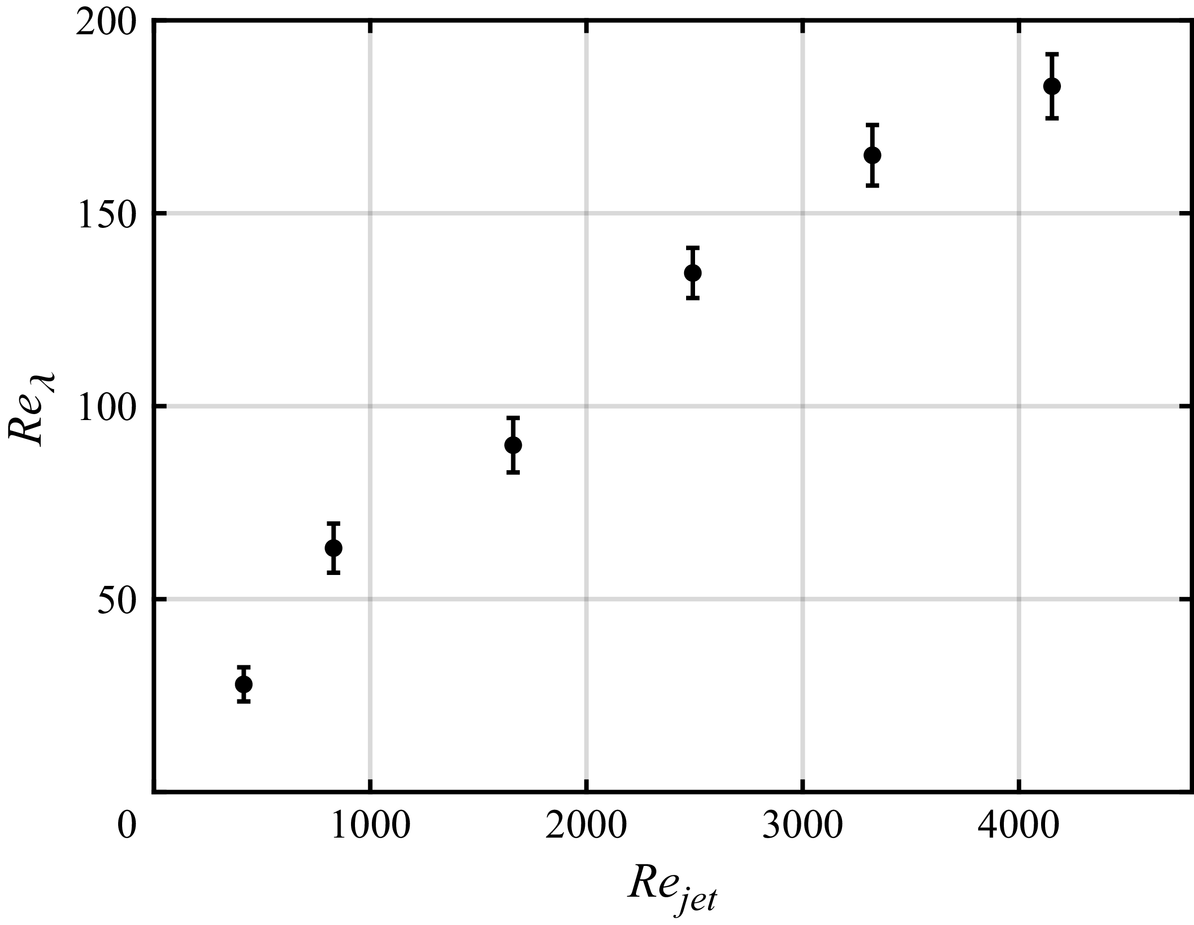
Since $\textit{Re}_{\textit{jet}}$ characterises the Reynolds number of the jet at the nozzle located at the corner of the container, it cannot fully represent the flow state after jet mixing in the central region of the container. Therefore, the Taylor microscale Reynolds number, $\textit{Re}_\lambda = \lambda u_{\textit{rms}} / \nu$ , in the HIT region is further evaluated and shown in figure 7. Here $\lambda = \sqrt {15 \nu u_{\textit{rms}}^2 / \varepsilon }$ is the Taylor microscale, $\varepsilon = 2\nu \langle s_{ij} s_{ij} \rangle$ is the turbulence dissipation rate, with $s_{ij} =( {1}/{2}) (\partial _{\!j} u_i + \partial _i u_{\!j})$ the strain-rate tensor. To account for the smallest dissipative eddies unresolved by the measurements, an approach analogous to large-eddy simulation was employed, in which the subgrid-scale (SGS) dissipation, $\varepsilon _{\textit{SGS}}=\langle 2 \nu _t s_{ij} s_{ij}\rangle$ , was modelled using the dynamic Smagorinsky model (Smagorinsky Reference Smagorinsky1963; Germano et al. Reference Germano, Piomelli, Moin and Cabot1991; Sheng et al. Reference Sheng, Meng and Fox2000). Here, $\nu _t= C_d \varDelta _g^2 (2 s_{ji}s_{ij})^{1/2}$ is the eddy viscosity and $\varDelta _g$ is the size of grids, where $\varDelta _g=\varDelta =0.3$ mm. The specific procedure used to calculate the dynamic coefficient $C_d$ from the experimentally obtained two-dimensional velocity field, as well as the convergence of the dynamic model in the present study, are discussed in detail in Appendix A. The corrected turbulent dissipation rate is then given by

(2.2) \begin{equation} \varepsilon = 2\nu \langle s_{ij} s_{ij} \rangle + \varepsilon _{\textit{SGS}}. \end{equation}

Under all experimental conditions, $\textit{Re}_\lambda$ increases with $\textit{Re}_{\textit{jet}}$ and falls within the range $\textit{Re}_\lambda \in [28, 183]$ .

Figure 7.

Taylor microscale Reynolds number $\textit{Re}_{\lambda }$ in the HIT area.

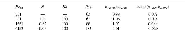
Under a strong magnetic field, the MHD effect introduces anisotropy into the driven turbulence, which serves as the initial condition for the decay problem and may influence the decay process. To assess this effect, experiments involving continuously driven turbulence under magnetic fields were conducted. Three representative conditions – high $N$ ( $N=1.28$ ), medium $N$ ( $N=0.62$ ) and low $N$ ( $N=0.08$ ) – were selected as initial fields for the decay studies. To control the effects of large-scale viscosity, the Hartmann number was fixed at $Ha = BL_0\sqrt {\sigma /\rho \nu } \approx 100$ . An experiment without a magnetic field was also conducted. The detailed parameters for these conditions are given in table 1. As shown in table 1, for each $N$ , the difference between $u_{y,\textit{rms}}$ and $u_{z,\textit{rms}}$ is less than 6 %, and the correlation functions normalised by $(u_{y,\textit{rms}}u_{z,\textit{rms}})$ are all less than 0.05. Thus, the anisotropy induced by the MHD effect does not significantly affect the isotropy of the initial field (Hwang & Eaton Reference Hwang and Eaton2004; Tan et al. Reference Tan, Xu, Qi and Ni2023; Gorce & Falcon Reference Gorce and Falcon2024).

Table 1.

Parameters for the experimental conditions at different $N$ .

Table 1. Long description

A table with six rows and seven columns comparing parameters for different experimental conditions. The columns are labeled Re_jet, N, Ha, Re_lambda, u_y,rms/u_z,rms, and u_y,u_z/(u_y,rms,u_z,rms). The rows present the following data: Row 1: Re_jet, 831; N, —; Ha, —; Re_lambda, 63; u_y,rms/u_z,rms, 0.99; u_y,u_z/(u_y,rms,u_z,rms), 0.019. Row 2: Re_jet, 831; N, 1.28; Ha, 100; Re_lambda, 62; u_y,rms/u_z,rms, 1.06; u_y,u_z/(u_y,rms,u_z,rms), 0.038. Row 3: Re_jet, 1661; N, 0.62; Ha, 100; Re_lambda, 88; u_y,rms/u_z,rms, 1.03; u_y,u_z/(u_y,rms,u_z,rms), 0.044. Row 4: Re_jet, 4153; N, 0.08; Ha, 100; Re_lambda, 183; u_y,rms/u_z,rms, 1.01; u_y,u_z/(u_y,rms,u_z,rms), 0.020.

Finally, to ensure the repeatability of the observations and reduce the influence of potential random errors, all decay experiments were repeated 10 times. The time-resolved results shown below are obtained by averaging over the 10 repeated experiments.

4.1. Anisotropic dissipation of the integrated kinetic energy

From the definition of $D_{\!j}$ (equation (3.4)), the directional dependence could be observed, which may lead to anisotropic decay of the velocity components perpendicular and parallel to the magnetic field. Therefore, the ratios of the squared velocity components perpendicular to and parallel to the magnetic field, $\varGamma = \langle u_{\!y}^2 \rangle / \langle u_z^2 \rangle$ , are shown in figure 9(a). At $N=1.28$ , $\varGamma$ increases during the initial decay stage and reaches its maximum value of $\varGamma = 1.54$ at $t^* \approx 1$ , after which it gradually decreases to unity. Figure 9(b) visually depicts this process through scatter plots of the velocity components perpendicular to and parallel to the magnetic field. Circular scatter-plot outlines indicate isotropy, while elongated circular outlines indicate anisotropy.

Figure 9.

Anisotropic decay of the velocity components at $N=1.28$ . (a) Ratio $\varGamma = \langle u_{\!y}^2 \rangle / \langle u_z^2 \rangle$ . (b) Scatter plots of $u_{\!y}$ and $u_z$ (normalised by maximum velocity).

The evolution of the ratio and scatter plots suggests that during the decay process, the HIT first becomes anisotropic and then gradually returns to isotropy. By comparing the evolution trends of the various dissipation terms shown in figure 8(b), it can be observed that the stage during which turbulence tends towards anisotropy corresponds to a regime of strong Joule dissipation, whereas the stage of recovery towards isotropy is dominated by viscous dissipation. In both stages, the energy flux remains relatively weak. These observations suggest that Joule dissipation promotes the development of anisotropy in turbulence, whereas viscous dissipation may be associated with the restoration of isotropy. During the phase of stronger energy injection, the turbulence remains approximately isotropic to some extent, suggesting that energy inflow in this stage may contribute to maintaining isotropy. Meanwhile, the recovery of isotropy corresponds to the stage in which the relative contribution of Joule dissipation increases and becomes comparable to that of viscous dissipation in the late decay phase, as shown in figure 8(b). This suggests that the transient anisotropy may contribute to the temporary dominance of viscous dissipation during part of the decay process. Specifically, the `preferential damping’ induced by Joule dissipation preferentially consumes the perpendicular component $u_z$ in the early stage, resulting in a decrease in the energy proportion of $u_z$ , as shown in figure 9(a). However, viscous dissipation acts on both $u_{\!y}$ and $u_z$ simultaneously, rendering the impact of the reduced $u_z$ energy on viscous dissipation less pronounced than on Joule dissipation, and thereby leading to a relative decrease in the proportion of Joule dissipation, as shown in figure 8(b). Subsequently, since the energy of $u_{\!y}$ exceeds that of $u_z$ , it experiences stronger viscous dissipation and decays more rapidly until it reaches a level comparable to $u_{z}$ , at which point the turbulence restores isotropy. The diminishing energy proportion of $u_y$ results in a relative decrease in the contribution of viscous dissipation. Finally, as isotropy is restored, Joule and viscous dissipations are of equal importance.

Furthermore, when $N=0.62$ , the evolution trend of $\varGamma$ is similar to that observed for $N=1.28$ , although its magnitude remains relatively smaller, with a maximum value of $\varGamma = 1.27$ , as shown in figure 9(a). As discussed in § 3, the evolution of Joule dissipation and viscous dissipation during the decay process at $N=0.62$ follows a pattern similar to that observed at $N=1.28$ . This similarity provides a plausible explanation for the comparable evolution behaviour of $\varGamma$ in the two cases. Finally, for $N=0.08$ , although Joule dissipation remains significantly weaker than viscous dissipation (figure 8 d), weak anisotropy still emerges relative to the case without a magnetic field, with a maximum $\varGamma =1.08$ .

4.2. Anisotropic evolution of energy spectrum

Ratio $\varGamma$ captures only the anisotropic evolution of the integral energy components $\langle u_{\!y}^2 \rangle$ and $\langle u_z^2 \rangle$ of the turbulent field. The influence of Joule dissipation on velocity components in different directions and at different scales needs to be characterised instead using two-dimensional energy spectra $\boldsymbol{\varPhi }(\boldsymbol k)$ . Since $\varGamma$ exhibits similar evolution across different $N$ values, and the development of anisotropy undergoes similar underlying physical processes, the case $N=1.28$ , where anisotropy is most pronounced, is selected for further analysis. The corresponding two-dimensional energy spectra in plane $\mathcal{P}$ and plane $\mathcal{V}$ at different times are shown in figures 10(a) and 10(b), respectively. Meanwhile, figure 10(c) presents the non-magnetic-field case, which is used as a reference for comparison. Here $\varphi (\boldsymbol k,\boldsymbol x)$ and $\varphi (\boldsymbol k,\boldsymbol y)$ denote the angles between the wavevector $\boldsymbol k$ and the $x$ axis (in plane $\mathcal{V}$ ) and the $y$ axis (in plane $\mathcal{P}$ ), respectively. It should be noted that, due to the resolution limitations of the PIV system, regions where $\boldsymbol{\varPhi }(\boldsymbol k)\lt 3\times 10^{-9}$ are strongly affected by measurement noise. As a result, the contours of $\boldsymbol{\varPhi }(\boldsymbol k)$ at large $k$ become sparse when $t^*\gt 1$ . This does not reflect the true distribution of $\boldsymbol{\varPhi }(\boldsymbol k)$ ; rather, it indicates that $\boldsymbol{\varPhi }(\boldsymbol k)\lt 3\times 10^{-9}$ in these regions.

Figure 10.

Temporal evolution of the two-dimensional energy spectrum $\boldsymbol{\varPhi }(\boldsymbol k)$ during decay at (a) $N=1.28$ , plane $\mathcal{P}$ ; (b) $N=1.28$ , plane $\mathcal{V}$ ; (c) no magnetic field. A common colour scale is used for all cases at each time instant.

At $t^*=0$ , the contours of $\boldsymbol{\varPhi }(\boldsymbol k)$ in all three cases exhibit an approximately circular distribution, indicating that the turbulence in the initial stage of decay is close to isotropic.

Subsequently, at $t^*=1$ , corresponding approximately to the stage at which anisotropy is strongest as shown in figure 9(a), clear anisotropy is also observed in the two-dimensional energy spectrum of plane $\mathcal{P}$ . Specifically, the contours of $\boldsymbol{\varPhi }(\boldsymbol k)$ become approximately elliptical, with the major axis aligned along $\theta =\pi /2$ , and this anisotropy is observed across almost all resolved scales. This result indicates that wavevectors perpendicular to the magnetic field retain more energy, whereas wavevectors with smaller $\theta$ exhibit lower energy and are more strongly affected by Joule dissipation, as shown in (3.4). Meanwhile, the energy spectrum in plane $\mathcal{V}$ remains approximately isotropic. However, compared with the case without a magnetic field, the contours shift towards smaller $k$ , indicating a larger gradient of the energy spectrum. This phenomenon reflects the steepening of the energy spectrum induced by Joule dissipation. Furthermore, in plane $\mathcal{P}$ , at $\theta =\pi /2$ , the gradient of $\boldsymbol{\varPhi }(\boldsymbol k)$ is closer to that of the case without a magnetic field, whereas at $\theta =0$ , it is nearly identical to that in plane $\mathcal{V}$ . This indicates that the steepening of the energy spectrum primarily occurs in wavevectors aligned with the magnetic field direction.

Then, at $t^*=3$ , the contours of $\boldsymbol{\varPhi }(\boldsymbol k)$ in plane $\mathcal{P}$ become more circular compared with those at $t^*=1$ , suggesting a weakening of anisotropy. This is consistent with the isotropy recovery process shown in figure 9(a). However, relatively strong energy is still retained at wavenumbers corresponding to $\theta =\pi /2$ . Meanwhile, $\boldsymbol{\varPhi }(\boldsymbol k)$ remains approximately isotropic in plane $\mathcal{V}$ as well as in the absence of a magnetic field, whereas the energy spectrum in plane $\mathcal{V}$ exhibits a steeper gradient.

Finally, at $t^*=10$ , $\boldsymbol{\varPhi }(\boldsymbol k)$ in plane $\mathcal{P}$ does not fully recover isotropy. On the one hand, wavevectors near $\theta =\pi /2$ still retain relatively high energy; on the other hand, strong energy emerges at small $k$ near $\theta =0$ . Unlike at $t^*=1$ , the distribution of $\boldsymbol{\varPhi }(\boldsymbol k)$ in plane $\mathcal{P}$ at $\theta =\pi /2$ deviates from that of the case without a magnetic field, and the overall energy is relatively lower. Since Joule dissipation does not directly act on wavevectors at $\theta =\pi /2$ (because $\cos ^2{( \pi /2)}=0$ in (3.4), the contribution from this term becomes zero), this difference should arise from mechanisms other than Joule dissipation. Meanwhile, the gradient of $\boldsymbol{\varPhi }(\boldsymbol k)$ is larger than that in plane $\mathcal{P}$ at $\theta =0$ , and it also exhibits higher energy at small wavenumbers. This difference may primarily arise from the distinct spatial structures of $u_z$ in plane $\mathcal{P}$ .

In summary, in plane $\mathcal{P}$ , $\ \boldsymbol{\varPhi }(\boldsymbol k)$ undergoes a process of first developing anisotropy and then gradually recovering towards isotropy. However, unlike the results in § 4.1, where turbulence nearly recovers isotropy in the final decay stage, $\boldsymbol{\varPhi }(\boldsymbol k)$ still exhibits observable anisotropy. This anisotropy originates from differences in the energy distribution along $k$ at different $\theta$ values and suggests the possible anisotropy of the turbulent structure. Therefore, the isotropic energy recovery process discussed in § 4.1 applies only to integral energy components. Meanwhile, $\ \boldsymbol{\varPhi }(\boldsymbol k)$ in both plane $\mathcal{V}$ and the non-magnetic-field case remains approximately isotropic throughout the decay process, while $\boldsymbol{\varPhi }(\boldsymbol k)$ in plane $\mathcal{V}$ exhibits a steeper gradient. It is noteworthy that, during the early decay stage ( $t^*=1$ ), the distributions of $\boldsymbol{\varPhi }(\boldsymbol k)$ in plane $\mathcal{P}$ at $\theta =\pi /2$ and $\theta =0$ are approximately consistent with the corresponding distributions of $\boldsymbol{\varPhi }(\boldsymbol k)$ as a function of $k$ in the non-magnetic-field case and in plane $\mathcal{V}$ , respectively. However, significant deviations emerge in both cases during the later decay stage ( $t^*=10$ ). The causes of these deviations and the anisotropic evolution of the turbulent structure are further discussed in subsequent sections.

5.1. Angular energy transfer

In plane $\mathcal{P}$ , $\boldsymbol{\varPhi }(\boldsymbol k)$ exhibits a non-uniform distribution across different $\theta$ , with higher energy at $\theta =\pi /2$ . This suggests the possible existence of organised energy transfer along the angular direction. This also provides a plausible explanation for why, in § 4.2, the overall energy of $\boldsymbol{\varPhi }(\boldsymbol k)$ at $\theta =\pi /2$ in plane $\mathcal{P}$ is lower than that in the non-magnetic-field case during the later stages of decay. An efficient approach to investigating energy fluxes in Fourier space is the ‘mode-to-mode’ energy transfer framework (Domaradzki & Rogallo Reference Domaradzki and Rogallo1990), which has been extensively applied to study the anisotropic energy fluxes induced by MHD effects (Dar et al. Reference Dar, Verma and Eswaran2001; Alexakis et al. Reference Alexakis, Mininni and Pouquet2005; Teaca et al. Reference Teaca, Verma, Knaepen and Carati2009; Reddy et al. Reference Reddy, Kumar and Verma2014; Fan et al. Reference Fan, Chen and Ni2025). For a triad $(\boldsymbol{k}, \boldsymbol{p}, \boldsymbol{q})$ , the energy transfer rate between modes is given by

(5.1) \begin{equation} S(\boldsymbol k|\boldsymbol p|\boldsymbol q)=\text{Im}\{\left [\boldsymbol k \boldsymbol{\cdot }\hat {\boldsymbol u}(\boldsymbol q)\right ] \left [\hat {\boldsymbol u}^*(\boldsymbol k) \boldsymbol{\cdot }\hat {\boldsymbol u}(\boldsymbol p)\right ]\}, \end{equation}

where $\text{Im}$ denotes the imaginary part and the asterisk represents the complex conjugate. This quantity describes the energy transfer from mode $\boldsymbol{p}$ to mode $\boldsymbol{k}$ , mediated by mode $\boldsymbol{q}$ , with $\boldsymbol{k} = \boldsymbol{p} + \boldsymbol{q}$ .

Following (5.1), the angular energy transfer $\varPi (\theta )$ can be defined (Reddy et al. Reference Reddy, Kumar and Verma2014) to investigate anisotropic energy dynamics. As shown in figure 11(a), for a specific angle $\theta$ between the wavevector and the magnetic field, $\varPi (\theta )$ represents the energy transferred from wavevectors $\boldsymbol{p}$ with $\theta ^* \lt \theta$ (the $G$ region) to wavevectors $\boldsymbol{k}$ with $\theta ^* \gt \theta$ (the $R$ region) in plane $\mathcal{P}$ :

(5.2) \begin{equation} \varPi (\theta )=\sum _{\boldsymbol k \in R}\sum _{\boldsymbol p \in G}S(\boldsymbol k|\boldsymbol p|\boldsymbol q). \end{equation}

The Fourier space is divided into 18 equally spaced angular sectors for $\theta \in (0, \pi /2)$ . A sharp cutoff was also applied to the velocity field with a cutoff wavenumber $k_c=0.3k_{\textit{max}}$ . Since only 2D-2C data were collected in this study, the results obtained from (5.2) can only directly reflect the angular energy transfer within plane $\mathcal{P}$ . However, figure 10(b) shows that isotropy in plane $\mathcal{V}$ is well preserved throughout the decay process, suggesting that the energy spectrum in plane $\mathcal{P}$ remains approximately symmetric about the $y$ axis. Therefore, although (5.2) does not provide the exact angular energy transfer of the full three-dimensional turbulent field, it may still capture its general behaviour and exhibit a similar evolution trend.

Figure 11.

(a) A schematic diagram for describing the definition of angular energy transfer $\varPi (\theta )$ . (b) Angular energy transfer $\varPi (\theta )$ at different decay times for $N=1.28$ (normalised by maximum absolute value).

Results at different times during the decay process for $N=1.28$ are shown in figure 11(b). Energy transfer $\varPi (\theta ) \lt 0$ , indicating that energy is transferred from wavevectors with larger $\theta$ to those with smaller $\theta$ , consistent with the distribution of $\boldsymbol{\varPhi }(\boldsymbol k)$ shown in figure 10(a). This indicates the indirect effect of Joule dissipation on wavevectors perpendicular to the magnetic field direction. Specifically, by directly dissipating the energy of wavevectors with $\theta \lt \pi /2$ , Joule dissipation induces angular energy inhomogeneity. This subsequently drives organised angular energy transfer, removing energy from wavevectors at $\theta \to \pi /2$ , and ultimately causes $\boldsymbol{\varPhi }(\boldsymbol k)$ in this direction to deviate from the non-magnetic-field case. Furthermore, as shown in figure 11(b), angular energy transfer gradually concentrates around $\theta \to \pi /2$ , which is similar to the conical energy flux identified by Fan et al. (Reference Fan, Chen and Ni2025). This suggests that, during the decay process, angular energy inhomogeneity gradually becomes concentrated near $\theta \to \pi /2$ .

5.2. Bidirectional energy transfer

One possible explanation for the strong large-scale (small $k$ ) energy observed near $\theta =0$ in plane $\mathcal{P}$ , as shown in figure 9(a), is that the energy in this region is not entirely transferred forward to smaller scales. Instead, a possible inverse energy transfer towards larger scales may occur. The bidirectional energy transfer has been confirmed in numerical simulations of decaying and forced MHD turbulence (Knaepen & Moreau Reference Knaepen and Moreau2008; Fan et al. Reference Fan, Chen and Ni2025) and also observed in laboratory experiments by Baker et al. (Reference Baker, Pothérat, Davoust and Debray2018); see also Alexakis & Biferale (Reference Alexakis and Biferale2018) for a review. Following (5.1), for a specific wavenumber $k_0 \in k$ , the net energy transfer from large scales ( $|\boldsymbol{p}| \lt k_0$ ) to small scales ( $|\boldsymbol{k}| \gt k_0$ ) across this wavenumber is

(5.3) \begin{equation} \varPi _T(k_0)=\sum _{|\boldsymbol k| \gt k_0}\sum _{|\boldsymbol p| \lt k_0}S(\boldsymbol k|\boldsymbol p|\boldsymbol q). \end{equation}

A positive $\varPi _T(k_0)$ indicates direct energy transfer, whereas a negative value signifies inverse energy transfer. Furthermore, strong large-scale energy is primarily concentrated in the region where $\theta \sim 0$ , corresponding to the $z$ -direction component in physical space. Therefore, to distinguish the different effects of the magnetic field on energy transport in the $y$ and $z$ directions, $\varPi _T(k_0)$ is decomposed into $y$ and $z$ components:

(5.4) \begin{align}\varPi _T(k_0)_{y}=\sum _{|\boldsymbol k| \gt k_0}\sum _{|\boldsymbol p| \lt k_0}\mathfrak{I} \big\{\big [\boldsymbol k \boldsymbol{\cdot }\hat {\boldsymbol u}(\boldsymbol q)\big ] \big [\hat {\boldsymbol u_{\!y}}^*(\boldsymbol k) \boldsymbol{\cdot }\hat {\boldsymbol u_{\!y}}(\boldsymbol p)\big ] \big\},\end{align}

(5.5) \begin{align}\varPi _T(k_0)_{z}=\sum _{|\boldsymbol k| \gt k_0}\sum _{|\boldsymbol p| \lt k_0}\mathfrak{I} \big\{\big [\boldsymbol k \boldsymbol{\cdot }\hat {\boldsymbol u}(\boldsymbol q)\big ] \big [\hat {\boldsymbol u_z}^*(\boldsymbol k) \boldsymbol{\cdot }\hat {\boldsymbol u_z}(\boldsymbol p)\big ]\big\}.\end{align}

A sharp cutoff was also applied to the velocity field with a cutoff wavenumber $k_c=0.3k_{\textit{max}}$ .

The $y$ and $z$ components of the energy flux, $\varPi _T(k_0)_{y}$ and $\varPi _T(k_0)_{z}$ , respectively, at different times during the decay process for $N=1.28$ are shown in figures 12(a) and 12(b). Figure 12(a) indicates that, in the direction parallel to the magnetic field, energy is primarily transferred directly at small scales ( $k_0 \gtrsim 600\ \mathrm{m}^{-1}$ ), with a weaker direct transfer also present at large scales. Meanwhile, as shown in figure 12(b), although $\varPi _T(k_0)_{z}$ still exhibits significant direct transfer at small scales, inverse energy transfer is observed at large scales ( $k_0 \lesssim 600\ \mathrm{m}^{-1}$ ). Unlike the direct energy flux, the inverse energy flux does not decrease significantly over time. This behaviour suggests that the relative contribution of inverse energy transfer gradually increases during the decay process, distinguishing it from the anisotropy pattern induced by Joule dissipation discussed in § 4. Therefore, the inverse transfer of $\varPi _T(k_0)_{z}$ towards larger scales is more likely to give rise to another MHD effect: $u_z$ components tend to develop larger-scale flow structures in directions perpendicular to it ( $y$ axis), manifested as vortex structures stretched along the magnetic field direction.

Figure 12.

Inter-wavenumber energy flux $\varPi _{T}(k_0)$ at different decay times for $N=1.28$ (cube-root-scaled for visualisation). (a) Parallel component. (b) perpendicular component.