NOMENCLATURE
- a ∞
-
freestream speed of sound, ms−1
- ai
-
ith-order isentropic contribution to the pressure-coefficient perturbation
- aie
-
entropy-related contribution to the pressure-coefficient perturbation
- b′ i
-
ith-order isentropic contribution to the perturbation velocity
- bi
-
ith-order entropy-related contribution to the pressure coefficient
- bie
-
entropy-related contribution to the pressure coefficient
- ci
-
terms in closed-form shock-angle relation
- cp
-
pressure coefficient, cp = (p − p ∞)/q ∞
- C
-
defined in Equation (33)
- CFD
-
computational fluid dynamics
- e
-
defined in Equation (34)
- li
-
ith-order contribution to the rise in entropy-ratio
- Li
-
grouping of linear coefficients of
 $\skew{-0.5}\hat{\phi }_{ii}$
, where i is the coordinate x or z
- m
-
$\sqrt{{\rm M}_\infty ^2 - 1}$
- M∞
-
freestream Mach number
- M2
-
Mach number following a Prandtl-Meyer expansion
- Ni
-
grouping of non-linear coefficients of
$\skew{-0.5}\hat{\phi }_{ii}$
, where i is the coordinate x or z
- p
-
fluid pressure, Pa
- q ∞
-
freestream dynamic pressure, Pa
- s
-
entropy, J/K
- u
-
x-component of the full perturbed velocity, m/s
- V ∞
-
freestream velocity, m/s
- V
-
full perturbed velocity, m/s
- w
-
z-component of the full perturbed velocity, m/s
- x
-
coordinate parallel to the freestream, m
- X 1
-
defined in Equation (37)
- X 2
-
defined in Equation (38)
- z
-
coordinate perpendicular to the freestream, m
- Z
-
defined in Equation (39)


Greek Symbol
- γ
-
ratio of specific heats
- Δpe
-
change in pressure coefficient associated with entropy, Pa
- Δprot
-
change in pressure coefficient associated with flow rotationality, Pa
- ΔVcurv
-
change in perturbation velocity associated with aerofoil curvature, m/s
- ΔVe
-
change in perturbation velocity associated with entropy, m/s−1
- δ
-
local flow turning angle, rad
- δdet
-
shock detachment angle, rad
- δvac
-
maximum flow turning angle, rad
- ε
-
measure of smallness of relative term magnitudes
- θ
-
shock angle, rad
- ν
-
Prandtl-Meyer function
-
$\skew{-0.5}\hat{\phi }$
-
perturbation potential function, m2/s
- ψ
-
defined in Equation (19)

Subscripts
- ()∞
-
freestream quantity
- ()donov
-
quantities evaluated through approximate relations
- ()exact
-
quantities evaluated through exact relations
- () x
-
derivative in x-direction
- () z
-
derivative in z-direction
1.0 INTRODUCTION
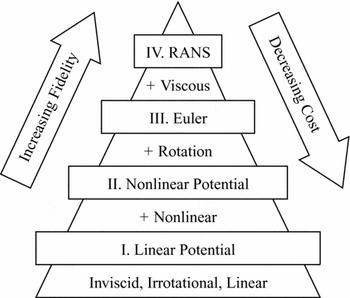
The increase in computing power over the past two decades has made the use of high-fidelity modelling in Computational Fluid Dynamics (CFD) increasingly affordable. This has allowed for complex flow phenomena to be modelled; however, the use of high-fidelity models in computing relatively simple flows may yield a very low increment in modelling accuracy while incurring significant expense. The balance between computational cost and modelling fidelity is particularly important in engineering tasks involving large numbers of computations or cases to be analysed, such as aeroelastic studies or design optimisation in the conceptual design stage. The complexity of the mathematical model used in the analysis must be appropriate to the complexity of the physics involved (see Fig. 1). The use of a lower-order mathematical model is generally appropriate for simple flows, or when the contribution from the neglected physics is not of interest. Examples of such simple supersonic flows include conical flows, as may be encountered over a sharp cone or delta-wing at near-zero incidence, and planar flows around corners, as occur over wedges and sharp-nosed aerofoils. These examples are characterised by attached shocks and small, attached boundary layers, and hence, the analytical inviscid models describing these flows are typically accurate. These restrictive conditions may still be encountered (at least approximately) in practical applications such as missiles at near-zero incidence, the lifting surfaces of supersonic aircraft in level flight, and supersonic air intakes. An example of a scenario in which the contribution from the physics neglected by lower-order models may not be of great interest is the supersonic aeroelasticity of a sharp aerofoil: the skin-friction drag and boundary layer may be of little interest to an aeroelastician concerned with normal forces and pitching moments acting on the profile.
Hierarchy of flow models, adapted from Jameson(Reference Jameson2).

Linear potential-flow methods have a long history of use in aeroelasticity and continue to receive attention(Reference Dowell and Bliss1) in literature. Their linear formulation allows the superposition of fundamental potential flows, such as doublets and horseshoe vortices, to describe the flow around general three-dimensional bodies. Linearity of the aerodynamic forces also facilitates their expression in the frequency domain and makes the aeroelastic system amenable to solution by methods for linear time-invariant systems. However, potential-flow methods are limited in the physics which they model. With reference to Fig. 1, it is seen that the more general description of physics offered by the Navier-Stokes equations is successively simplified in reduction to the linear potential-flow formulation, with mathematical terms modelling viscous effects, rotationality and non-linearity being discarded. These terms become increasingly important in the transonic and hypersonic regimes for flows with detached or curved shocks, and for geometries with large curvature and flow separation. It can therefore not be expected that linear potential-flow methods will yield an accurate result under such conditions. Nonetheless, they remain valuable in the aeroelastic analysis of aircraft at supersonic speeds.
Justification of the successive simplification in the mathematical models used to model the flow physics as described above may be made through two different approaches. One approach is to solve the problem defined by the particular geometry and freestream parameters using flow models of differing fidelity (e.g. non-linear potential vs linear potential formulation) and to compare the results of the final solutions. While this approach provides a rigorous basis for simplification in terms of the results of interest, it is costly in requiring the problem to be solved using more than one model. Furthermore, the solution will generally not be linearly dependent on the parameters involved, and the justification would need to be repeated for a problem with a different set of parameters. The second approach to justifying the simplification of the mathematical model lies in an a-priori consideration of the relative order of terms in a non-dimensionalised formulation of the governing equations. Terms which are identified to be of a sufficient order smaller than the rest are neglected, leading to a simplification of the mathematical formulation. While this approach does not compare the differences in the solution of the simplified flow models, it offers the advantage of being general, and effectively has no computational cost associated with it, as no solution is required.
A disadvantage of the a-priori mathematical approach is the question of quantifiability. The development of simplified models and physical analogies is typically(Reference Meijer and Dala3) achieved through asymptotic development, in which terms are neglected through assumptions such as “small” perturbations and “sufficiently large” Mach numbers. Theoretical validity ranges for applying such models are often only defined as an asymptotic limit; quantitative ranges are typically empirically determined. The purpose of the present work is to provide a framework for quantifying non-linearity in planar supersonic potential flows in terms of the main parameters of interest, and hence, for determining a-priori the parameter space within which the simplifying assumptions made in linearising the potential flow equation are mathematically consistent or valid. This would serve to better inform the engineer of the conditions under which the application of analysis tools based in linear potential flows is no longer mathematically consistent, and of the probable error due to linearisation in the methods.
The present work offers a parameterisation of the non-linear terms in the full potential equation in terms of the freestream Mach number and the local flow turning angle. The relative magnitude of non-linear terms and term-groupings as quantified by the parameterisation is considered over the parameter space to give a quantitative estimate of the regions in which terms may be discarded to within a specified degree of error. The velocity perturbations are parameterised using expressions developed by Donov(Reference Donov4) for the velocity at the surface of an aerofoil. The accuracy of Donov’s method, which has not previously been quantified, is investigated in the present work by comparison to the exact solutions for an oblique shock over a wedge and for Prandtl-Meyer expansion around a corner.
The approach adopted in the present work of comparing non-linear and linear potential flow terms is similar to the analysis carried out by Cole(Reference Cole5) in assessing non-linearity in transonic flows for bodies of revolution, while the focus of the present work is planar flows. The a-priori justification for linearisation adopted here, by means of quantifying the relative magnitude of terms in the full potential equation, provides insight into the sources of non-linearity. This is absent from a justification based on the differences between models in the resulting pressure, as was adopted by Hilton(Reference Hilton6) in evaluating the limitations of Busemann’s(Reference Busemann7) second-order theory relative to a third-order model.
The paper is outlined as follows. Donov’s(Reference Donov4) method and the its key relations are introduced in Section 2, with their accuracy relative to exact relations being assessed in Section 3. The subsequent parameterisation of terms in the potential flow equation and non-linear term-groupings is presented in Section 4. The approach adopted in quantifying non-linearity and estimating the validity bounds of linear analysis is described in Section 5, followed by key conclusions in Section 6.
2.0 PRESSURE AND VELOCITY PERTURBATIONS
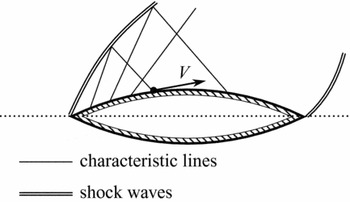
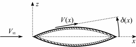
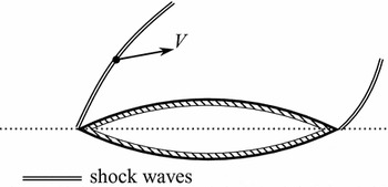
Donov(Reference Donov4) developed a number of power-series expressions for the flow velocity and pressure on an aerofoil surface. The aim of the work was to expand on existing expressions developed for isentropic, irrotational flows (as described in Section 2.1), and to obtain expressions which would account for the rotationality and entropy gradients in the flowfield between the leading-edge shock and the aerofoil surface (as presented in Section 2.3 and depicted in Fig. 2). The basis for Donov’s development was in the method of characteristics(Reference Anderson8) for two-dimensional steady flows, with the general formulation accounting for flow rotationality. This restricted the analysis to flows in which the flowfield was everywhere supersonic, and thereby does not permit application to bodies with detached shocks or embedded subsonic flows. No discussion was given of the expected validity bounds of the analysis in terms of Mach number or the flow turning angle, other than that perturbations were assumed to be “small”. The subsequent derivation of the expressions for velocity and pressure on the aerofoil surface was presented in three parts, which are outlined in the subsections; specifically, 2.1, 2.2, and 2.3 that follow. The nomenclature associated with the development is defined in Fig. 3.
General configuration considered.

Nomenclature adopted.

2.1 Isentropic flow over a shock-free aerofoil
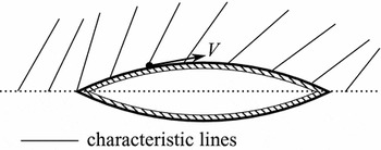
The first component of Donov’s(Reference Donov4) analysis related to the existing expressions for the isentropic flow over an aerofoil that would occur if no shocks are present in the entire flowfield, as in Fig. 4. The case of isentropic expansion from the freestream around a corner was presented first, with arguments for isentropic compressions made later. With the flowfield everywhere irrotational, the characteristic equations reduced to a form allowing analytical integration, and the familiar Prandtl-Meyer function was obtained. By means of a Taylor-series expansion about the freestream reference values (V = V ∞, p = p ∞, δ = 0), a power series for the flow velocity and pressure on the aerofoil surface was obtained in terms of M∞ and δ. The fluid pressure following an isentropic expansion or compression was expressed(Reference Donov4) as
 $$\begin{equation}
p = p_\infty + q_\infty \left[ a_1 \delta (x) + a_2 \delta ^2(x) + a_3 \delta ^3(x) + a_4 \delta ^4(x) + {\it O}(\delta ^5) \right] ,
\end{equation}$$
where the coefficients are given in the appendix, and
 $$\begin{equation*}
q_\infty = \frac{\gamma p_\infty {\rm M}_\infty ^2}{2}.
\end{equation*}$$
The corresponding flow velocity along the aerofoil was given(Reference Donov4) by
 $$\begin{equation}
V = V_\infty \left[ 1 + b_1^{\prime } \delta + b_2^{\prime } \delta ^2 + b_3^{\prime } \delta ^3 + b_4^{\prime } \delta ^4 + {\it O}(\delta ^5) \right] \quad \mbox{for}\quad \delta < 0.
\end{equation}$$
Donov(Reference Donov4) argued that for sufficiently small perturbations, the same equations could be used to model isentropic compressions, as might occur for smoothly- and slowly-turned flow. This argument was made from consideration of the oblique shock equations, which were part of the second tier of Donov’s development.
Shock-free isentropic flow.

2.2 Flow velocity behind an oblique shock
Having established the expressions for flow over an aerofoil which produces no shocks, Donov(Reference Donov4) turned to the treatment of the oblique shock that would be produced at the aerofoil leading edge, shown in Fig. 5. Power-series expressions for the flow velocity and entropy rise following an oblique shock were given, developed from the Euler equations. The expression used for the velocity behind an oblique shock in the second step of Donov’s(Reference Donov4) analysis was
 $$\begin{equation}
V = V_\infty \left[ 1 + b_1 \delta + b_2 \delta ^2 + b_3 \delta ^3 + b_4 \delta ^4 + {\it O}(\delta ^5) \right] \quad \mbox{for}\quad \delta > 0
\end{equation}$$
with coefficients listed in the appendix. The rise in entropy was described(Reference Donov4) by
 $$\begin{equation}
s = s_\infty \left[ 1 + l_3 \delta ^3 + l_4 \delta ^4 + {\it O}(\delta ^5) \right].
\end{equation}$$
Donov(Reference Donov4) noted that the rise in entropy and associated rotationality introduced by the shock entered only from third-order terms in δ and higher, concluding that for sufficiently small disturbances (and hence, small δ), the flow could be approximated as irrotational and isentropic. This would allow the same form of the characteristic equations as in the previous step to be integrated, and would allow the existing expressions for isentropic expansions, namely Equations (1) and (2), to be used for isentropic compressions.
Oblique leading-edge shock.

2.3 Rotational flow over an aerofoil with a leading-edge shock
Building on the expressions from the previous steps, Donov(Reference Donov4) constructed a solution for the flow properties at the aerofoil surface, which accounted for the entropy gradients between the shock produced by the leading edge and the aerofoil surface, originally depicted in Fig. 2. The mathematical details of the solution are not entered into here and are presented at length in Donov’s(Reference Donov4) original work. The crux of the procedure lies in the assumption of small perturbations and weak (but non-zero) rotationality; analytical integration of the approximate equations is then performed along characteristics. This sets the method apart from a lower-order “shock-expansion” approach in which isentropic expansion behind a straight shock is assumed; in Donov’s method, entropy gradients and curvature of the shock due to interaction with characteristics from the aerofoil surface are accounted for. Flow behind the leading-edge shock was modelled as being turned smoothly, with no further shocks forming.
The final product of the three-tiered development was a set of power-series expressions for p and V along the surface of an aerofoil with a rotational flowfield. Terms representing the increments relative to isentropic expansions and compressions (derived in the previous steps) were singled out, and terms specifically associated with vorticity behind the shock (Δprot ) and the curvature of the aerofoil immediately aft of the leading edge (Vcurv ) were identified.
The pressure on the aerofoil was given(Reference Donov4) as
 $$\begin{equation}
p = p_\infty + q_\infty \left[ a_1 \delta (x) + a_2 \delta ^2(x) + a_3 \delta ^3(x) + a_4 \delta ^4(x) \right] + \Delta p_e + {\it O}(\delta ^5) ,
\end{equation}$$
where the additional terms relative to the isentropic formulation of Equation (1) are given by
 $$\begin{equation}
\Delta p_e = q_\infty \left[ a_{1e} \delta ^{3}(0) + a_{2e} \delta ^{4}(0) + a_{3e} \delta ^{3}(0) \delta (x) \right] + \Delta p_{rot} \end{equation}$$\\
 $$\begin{equation}
\Delta p_{rot} = q_\infty \left[ a_{4e} x \delta ^{3}(0) \delta _{x}(0) \right].
\end{equation}$$
The result of Donov’s(Reference Donov4) integration along characteristics, given in Equation (5), is that the pressure distribution is essentially similar in form to that which the aerofoil would have if no leading-edge shock were formed, given by the isentropic formulation of Equation (1). The additional pressure distribution associated with the formation of the leading-edge shock and the subsequent entropy gradients and rotationality in the flowfield are given by the term Δpe . This term is seen to only contain terms in the third-order and higher of the flow turning angle at the leading edge, δ(0), with a fourth-order-smallness term involving the local flow turning angle, δ(x). Donov further isolated the contribution from vortex-formation as the term Δprot . It is seen to depend on the curvature δ x (0) of the aerofoil surface immediately aft of the sharp leading edge and to depend on the distance x from the leading edge. The coefficients ane (given in the appendix) associated with the additional term Δpe are seen to depend on both isentropic coefficients b′ n and on coefficients relating to flow behind the oblique shock, bn and ln ; this composition of the coefficients ane derives from the integration along characteristics between the shock and the aerofoil surface.
The flow velocity at the aerofoil surface as given by Donov(Reference Donov4) was similarly cast as
 $$\begin{equation}
V = V_\infty \left[1 + b_1^{\prime } \delta (x) + b_2^{\prime } \delta ^2(x) + b_3^{\prime } \delta ^3(x) + b_4^{\prime } \delta ^4(x) \right] + \Delta V_e + {\it O}(\delta ^5) ,
\end{equation}$$
where additional terms relative to the isentropic formulation of Equation (2) are given by
 $$\begin{equation}
\Delta V_e = V_\infty \left[ b_{1e} \delta ^3(0) + b_{2e} \delta ^4(0) + b_{3e} \delta ^3(0) \delta (x) \right] + \Delta V_{curv},
\end{equation}$$\\
 $$\begin{equation}
\Delta V_{curv} = V_\infty \left[ b_{4e} x \delta ^3(0) \delta _{x}(0) \right].
\end{equation}$$
3.0 PARAMETERISATION ACCURACY
The power-series expressions of Donov(Reference Donov4) may be compared to exact solutions for planar supersonic flows to assess the accuracy of Donov’s results: for isentropic expansion, Equations (1) and (2) may be evaluated against the exact solution of Prandtl-Meyer expansion; for oblique shocks, Equations (5) and (8) (evaluated for δ x (0) = 0) are compared to the Rankine-Hugoniot equations.
3.1 Exact relations
The pressure and velocity ratios following a Prandtl-Meyer expansion are manipulated from Anderson(Reference Anderson8) as
 $$\begin{equation}
\frac{p}{p_\infty } = \left[ \frac{2 + (\gamma - 1){\rm M}_\infty ^2}{2 + (\gamma - 1){\rm M}_2^2} \right]^{\gamma /(\gamma - 1)}
\end{equation}$$\\
 $$\begin{equation}
\frac{V}{V_\infty } = \frac{{\rm M}_2}{{\rm M}_\infty } \sqrt{ \frac{2 + (\gamma - 1){\rm M}_\infty ^2}{2 + (\gamma - 1){\rm M}_2^2} } ,
\end{equation}$$
 $$\begin{equation}
\nu ({\rm M}_2) = \nu ({\rm M}_\infty ) - \delta \quad \mbox{for}\quad \delta < 0
\end{equation}$$\\
 $$\begin{equation}
\nu ({\rm M}_\infty ) = \sqrt{e} \tan ^{-1}\left[ m / \sqrt{e} \right] - \tan ^{-1}(m)
\end{equation}$$\\
 $$\begin{equation}
m = \sqrt{{\rm M}_\infty ^2 - 1 }.
\end{equation}$$
 $$\begin{equation}
\frac{p}{p_\infty } = \frac{1}{e} \left( \frac{2\gamma }{\gamma - 1}{\rm M}_\infty ^2 \sin ^2\theta - 1 \right),
\end{equation}$$\\
 $$\begin{equation}
\frac{V}{V_\infty } = \frac{\sin \theta }{e \sin (\theta - \delta )} \left( \frac{2}{\gamma - 1}\frac{1}{{\rm M}_\infty ^2 \sin ^2\theta } + 1 \right) ,
\end{equation}$$
 $$\begin{equation}
\sin ^2 \theta = - \frac{c_1}{3} + \left[ \frac{2 \sqrt{c_1^2 - 3c_2}}{3}\right] \cos \left( \frac{\psi + 4\pi }{3} \right),
\end{equation}$$
where
 $$\begin{equation}
\cos \psi = \left( \frac{9}{2}c_1 c_2 - c_1^3 - \frac{27}{2}c_3 \right) / \left( c_1^2 - 3c_2 \right)^{3/2},
\end{equation}$$\\
 $$\begin{equation}
c_1 = - 1 - \gamma \sin ^2 \delta - (2/{\rm M}_\infty ^2),
\end{equation}$$\\
 $$\begin{equation}
c_2 = \frac{2{\rm M}_\infty ^2 + 1}{{\rm M}_\infty ^4} + \left[ \frac{(\gamma + 1)^2}{4} + \frac{\gamma - 1}{{\rm M}_\infty ^2} \right] \sin ^2 \delta ,
\end{equation}$$\\
 $$\begin{equation}
c_3 = - ( \cos ^2 \delta )/{\rm M}_\infty ^4.
\end{equation}$$
3.2 Relative accuracy of parameterised expressions
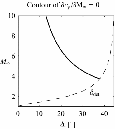
The results given by Donov’s(Reference Donov4) expressions as applied to a wedge or an isentropic expansion about a corner are compared to the exact solutions for these problems as given by the Rankine-Hugoniot relations for oblique shocks and the Prandtl-Meyer solutions. The relative error in the results using Donov’s equations is assessed for a range of Mach numbers and flow turning angles for which shocks remain attached (δ < δdet) and for which vacuum is not reached (δ > δvac). In considering the accuracy of the power-series expressions, it is worth keeping in mind the correlation of the mathematical expressions with physical phenomena. In particular, the pressure coefficient cp on a body is known to tend to a constant value in the hypersonic limit – this is known as the Mach independence principle. The power-series form of Equations (1) and (5) for pressure on the aerofoil surface is seen to introduce terms which become unbounded in the hypersonic limit when the series is developed to third-order or higher. The region of the parameter space in which the isentropic relation of Equation (1) gives a trend in cp consistent with physical phenomena (∂cp /∂M∞ ⩽ 0) is illustrated in Fig. 6. It should be noted that the pressure predicted by the relation outside of this range may still be close to the exact value of the Rankine-Hugoniot equations, and may still yield valuable estimations of the pressure despite yielding incorrect trends as the Mach number is increased further. An approximate relation for departure from the Mach independence principle for Equations (1) and (5) may be estimated as values of the hypersonic similarity parameter M∞δ > 2.
Limit of adherence of third-order isentropic pressure equation to the Mach independence principle.

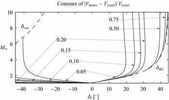
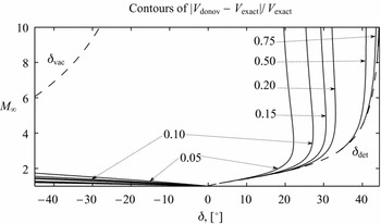
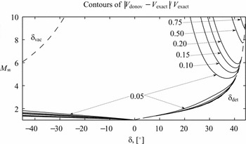
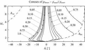
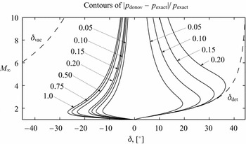
The error in velocity given by Donov’s(Reference Donov4) series, V donov, relative to the flow velocity given by the exact relations, V exact, is shown developed up to third-order in Figs 7-9: for expansion flows, Equations (2) and (12) are evaluated; for compression flows, Equations (8) and (17) are evaluated. Similarly, the error in pressure given by Donov’s(Reference Donov4) series, p donov, relative to that given by the exact relations, p exact, is shown in Figs 10-12: for expansion flows, Equations (1) and (11) are evaluated; for compression flows, Equations (5) and (16) are evaluated.
Accuracy of the velocity series relative to exact flow relations: first-order.

Accuracy of the velocity series relative to exact flow relations: second-order.

Accuracy of the velocity series relative to exact flow relations: third-order.

Accuracy of the pressure series relative to exact flow relations: first-order.

Accuracy of the pressure series relative to exact flow relations: second-order.

Accuracy of the pressure series relative to exact flow relations: third-order.

It is seen from Figs 7-9 that the expressions of Donov(Reference Donov4) for flow velocity are accurate to within 5% of the exact flow velocity for a large portion of the parameter space, while significant errors are encountered for compression flows with moderate turning (δ > 20°) near shock-detachment and in the hypersonic limit. No significant differences in velocity prediction are seen between the first-order and second-order expressions, except for near-vacuum expansion flows. Improved prediction for compression flows is achieved by extension to third-order expressions; however, this leads to the velocity in Equation (8) becoming unbounded in the limit of M∞ → ∞ due to the introduction of the O(M8 ∞ m −7) term of Equation (56).
Similar unboundedness is observed in Equations (1) and (5) for the fluid pressure, once again introduced from third-order terms through O(M8 ∞ m −7) in Equation (55); in the case of the pressure series, however, unboundedness is also observed for expansion flows. Notable improvement in the accuracy of the pressure series is seen in extension from first-order (Fig. 10) to second-order (Fig. 11); the improvement in accuracy is lost at large values of M∞ and δ when extension to third-order (Fig. 12) is made due to the divergence of the series. The relatively narrow band of the M∞-δ parameter space for which accurate pressures are obtained from the relation between local fluid pressure and local velocity, particularly as observed for Figs 10 and 11, is related to the assumptions made in similar methods employing local relations for pressure and velocity (Reference Meijer and Dala3), namely that the hypersonic similarity parameter M∞δ < 1.
The relative error in Donov’s(Reference Donov4) expressions for flow velocity may be used to qualitatively assess the accuracy of comparing the relative magnitudes of velocity perturbations in a potential flow formulation. As noted by Van Dyke(Reference Van Dyke11), the calculation of the perturbation velocities and of the perturbation pressure in a potential flow formulation are essentially two distinct operations, and so the pressure equation does not need to be simplified to solve the flow. Thus, the relative error in Donov’s(Reference Donov4) expressions for fluid pressure is not necessarily a reflection of the accuracy of the full pressure equation for potential flows as given by Equation (44).
In conclusion, the relative-magnitude analysis of perturbation velocities in the full potential equation to be conducted in the present work may be qualitatively estimated as valid for regions of the parameter space for which good agreement is obtained in the velocity prediction. From Figs 8 and 9, the analysis is estimated as valid for flow turning angles of δ < 20°; for large Mach numbers and similar or larger flow turning angles, the inherently non-linear region of hypersonic flows is entered, and the analysis may be considered as qualitative at best.
4.0 TERMS IN NON-LINEAR POTENTIAL FLOWS
4.1 Correlation to preceding expressions
The expressions of Donov(Reference Donov4) may be used to parametrise terms in a potential-flow framework in terms of Mach number, M∞, and flow turning angle, δ, allowing the magnitude of the terms to be quantified. The irrotationality assumed by a potential flow model may be consistently adhered to for both expansion and compression flow by employing terms up to second-order in δ from Donov’s series. Extension of the parameterisation to third-order is mathematically inconsistent with a potential-flow formulation when shocks are present; however, it allows an estimate to be made of the effect of entropy and rotationality relative to an O(δ3) isentropic formulation through Equation (9). In the present work, expressions will only be developed up to the third-order. A steady planar flow in the x-z plane is considered as in Fig. 4; the velocity components are formulated as
 $$\begin{equation}
u = V_\infty + \skew{-0.5}\hat{\phi }_{x} = V \cos \delta ,
\end{equation}$$\\
 $$\begin{equation}
w = \skew{-0.5}\hat{\phi }_{z} = V \sin \delta ,
\end{equation}$$
 $$\begin{equation}
\cos \delta = 1 - \delta ^2 /2 + {\it O}(\delta ^4),
\end{equation}$$\\
 $$\begin{equation}
\sin \delta = \delta - \delta ^3 /6 + {\it O}(\delta ^5).
\end{equation}$$
 $$\begin{equation}
\skew{-0.5}\hat{\phi }_{x} = V_\infty \left[ b_1\delta + (b_2 - 1/2)\delta ^2 + (b_3^{\prime } - b_1/2)\delta ^3 + {\it O}(\delta ^4) \right],
\end{equation}$$\\
 $$\begin{equation}
\skew{-0.5}\hat{\phi }_{z} = V_\infty \left[\delta + b_1\delta ^2 + (b_2 - 1/6)\delta ^3 + {\it O}(\delta ^4) \right].
\end{equation}$$
4.2 Terms considered in the full potential flow equation
In the absence of discontinuities in the flow, non-linearity arises when velocity perturbations may no longer be considered “small” and product terms such as
 $\skew{-0.5}\hat{\phi }_{x}\skew{-0.5}\hat{\phi }_{xx}$
must be considered. The full non-linear potential equation for steady planar flows is
 $$\begin{eqnarray}
(a_\infty ^2 - V_\infty ^2)\skew{-0.5}\hat{\phi }_{xx} + a_\infty ^2\skew{-0.5}\hat{\phi }_{zz} & = & \left[ (\gamma + 1)V_\infty \skew{-0.5}\hat{\phi }_{x} + (\gamma + 1)\skew{-0.5}\hat{\phi }_{x}^2/2 + (\gamma - 1)\skew{-0.5}\hat{\phi }_{z}^2/2 \right] \skew{-0.5}\hat{\phi }_{xx} \nonumber \\
& & +\, \left[ (\gamma - 1)V_\infty \skew{-0.5}\hat{\phi }_{x} + (\gamma - 1)\skew{-0.5}\hat{\phi }_{x}^2/2 + (\gamma + 1)\skew{-0.5}\hat{\phi }_{z}^2/2 \right] \skew{-0.5}\hat{\phi }_{zz} \nonumber \\
& & +\, 2(V_\infty + \skew{-0.5}\hat{\phi }_{x}) \skew{-0.5}\hat{\phi }_{z} \skew{-0.5}\hat{\phi }_{xz}.
\end{eqnarray}$$
The equation may be recast as follows, with terms leading to non-linearity grouped together
 $$\begin{equation}
(L_x - N_x)\skew{-0.5}\hat{\phi }_{xx} + (L_z - N_z)\skew{-0.5}\hat{\phi }_{zz} = C ,
\end{equation}$$
where
 $$\begin{equation}
L_x = -m^2,
\end{equation}$$\\
 $$\begin{equation}
L_z = 1,
\end{equation}$$\\
 $$\begin{equation}
C = 2[{\rm M}_\infty + (\skew{-0.5}\hat{\phi }_{x} / a_\infty )] (\skew{-0.5}\hat{\phi }_{z} / a_\infty ) \skew{-0.5}\hat{\phi }_{xz},
\end{equation}$$\\
 $$\begin{equation}
e = (\gamma + 1)/(\gamma - 1),
\end{equation}$$\\
 $$\begin{equation}
N_x = eX_1 + eX_2 + Z,
\end{equation}$$\\
 $$\begin{equation}
N_z = X_1 + X_2 + eZ,
\end{equation}$$\\
 $$\begin{equation}
X_1 = (\gamma - 1) {\rm M}_\infty \skew{-0.5}\hat{\phi }_{x}/ a_\infty ,
\end{equation}$$\\
 $$\begin{equation}
X_2 = (\gamma - 1) \skew{-0.5}\hat{\phi }_{x}^2/ 2 a_\infty ^2
\end{equation}$$\\
 $$\begin{equation}
Z = (\gamma - 1) \skew{-0.5}\hat{\phi }_{z}^2/ 2 a_\infty ^2.
\end{equation}$$
 $$\begin{equation}
X_1 = (\gamma - 1){\rm M}_\infty ^2 \left[ b_1\delta + (b_2 - 1/2)\delta ^2 + (b_3^{\prime } - b_1/2)\delta ^3 + {\it O}(\delta ^4) \right],
\end{equation}$$\\
 $$\begin{equation}
X_2 = (\gamma - 1){\rm M}_\infty ^2 \left[ b_1^2\delta ^2/2 + b_1(b_2 - 1/2)\delta ^3 + {\it O}(\delta ^4) \right] ,
\end{equation}$$\\
 $$\begin{equation}
Z = (\gamma - 1){\rm M}_\infty ^2 \left[ \delta ^2/2 + b_1\delta ^3 + {\it O}(\delta ^4) \right].
\end{equation}$$
 $$\begin{equation}
\frac{p}{p_\infty } = \left[ 1 + \frac{\gamma - 1}{2} {\rm M}_\infty ^2 \left( 1 - \frac{V^2}{V_\infty ^2} \right) \right]^{\gamma / (\gamma - 1)},
\end{equation}$$
which upon substitution of Equations (23), (24) and (37)-(42), together with V 2 = u 2 + w 2, yields
 $$\begin{equation}
p/p_\infty = \left( 1 - X_1 - X_2 -Z \right)^{\gamma /(\gamma - 1)}.
\end{equation}$$
It may be shown that upon expanding Equation (44) into a power series, and substituting Equations (40)–(42) and rearranging, Donov’s(Reference Donov4) expression for the fluid pressure following an isentropic expansion, as given by Equation (1), is recovered.
5.0 QUANTIFYING NON-LINEARITY
The parameterisation of the perturbation velocities at the wall in a planar system allows the terms that lead to non-linearity in Equation (30) to be quantified. These terms (X
1, X
2 and Z, scaled by e where appropriate) may be grouped together as an overall non-linear term, Ni
, in the coefficient of
 $\skew{-0.5}\hat{\phi }_{ii}$
. The magnitude of the term Ni
relative to the magnitude of the linear coefficient, Li
, of
 $\skew{-0.5}\hat{\phi }_{ii}$
may be perceived as a quantitative measure of the non-linearity associated with
 $\skew{-0.5}\hat{\phi }_{ii}$
. This, in turn, provides a numerical basis from which linearisation of the full potential equation at a particular range of M∞ and δ may be justified as mathematically consistent. Linearisation of Equation (30) is formally defined through the simultaneous assumptions that
 $$\begin{equation}
|N_x| \ll |L_x|,
\end{equation}$$\\
 $$\begin{equation}
|N_z| \ll |L_z|,
\end{equation}$$\\
 $$\begin{equation}
|C| \ll |(L_i - N_i)\skew{-0.5}\hat{\phi }_{ii}|,
\end{equation}$$
 $\skew{-0.5}\hat{\phi }_{ii}$
is the smaller of the streamwise and transverse terms. If a geometry with sufficiently small curvature, δ
x
= δ
x
(x), is considered, then, following from Equation (10), the contribution of curvature terms to the perturbation velocity are O(δ3(0)δ
x
(0)) and may be neglected in favour of lower-order contributions; hence, the term associated with curvature in the full potential equation, C, may be considered negligible compared to
 $(L_i - N_i)\skew{-0.5}\hat{\phi }_{ii}$
. In considering the negligibility of the non-linear terms Ni
away from the asymptotic limits of M∞ → 1 and M∞ → ∞ (in which linearised theory is invalid), the formal definition of “ ≪ ” must be dropped, and a quantitative threshold of acceptable “smallness” of the relative magnitudes of linear and non-linear terms must be adopted. Let this smallness parameter be denoted by ε. Having assumed that C will be negligible, linearisation of the full potential equation is then defined by the simultaneous conditions that
 $$\begin{equation}
|N_x / L_x| < \epsilon ,
\end{equation}$$\\
 $$\begin{equation}
|N_z / L_z| < \epsilon.
\end{equation}$$
Under these conditions, the full potential equation is reduced to the familiar linear potential equation of
 $$\begin{equation}
L_x\skew{-0.5}\hat{\phi }_{xx} + L_z\skew{-0.5}\hat{\phi }_{zz} = 0.
\end{equation}$$
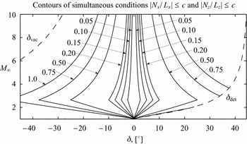
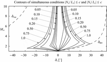
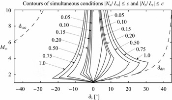
The contours in the M∞-δ parameter space, within which Equations (49) and (50) are simultaneously satisfied, are shown for a range of values of ε in Figs 13-15, with the non-linear terms, given by Equations (40)-(42), evaluated up to the first three orders of δ. Once again, the narrow band for which linearised theory is valid is observed along with the importance of higher-order terms in δ, as evidenced by the noticeable shift in contours when extending the analysis from O(δ) (Fig. 13) to O(δ2) (Fig. 14).
Relative contribution of non-linearity in the potential flow equation: first-order.

Relative contribution of non-linearity in the potential flow equation: second-order.

Relative contribution of non-linearity in the potential flow equation: third-order.

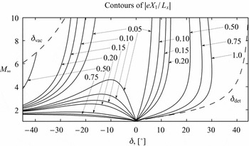
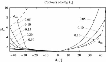
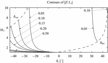
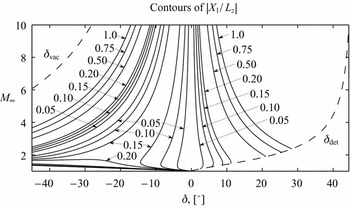
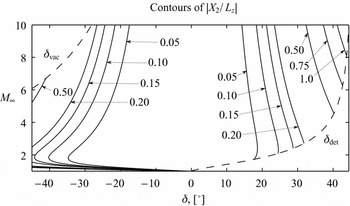
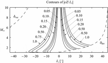
The contribution of the individual terms in the non-linear groupings Ni relative to the linear terms Li is shown in Figs 16-21, with the terms evaluated up to third-order in δ. It must be noted that the signs of the individual non-linear terms vary over the parameter space, and in certain regions are not of the same sign. This is particularly significant in considering the influence of |X 1/Lz | (Fig. 19) and of |eZ/Lz | (Fig. 21); the terms are of similar magnitude, but of opposite sign, and therefore, the net contribution to the non-linearity Nz of the otherwise significant individual terms may be small. In this regard, caution must be exercised to consider the relative magnitude of term groupings, rather than individual terms. Nonetheless, it may be concluded that over the majority of the parameter space, the contribution of the terms |eX 2/Lx |, |Z/Lx | and |X 2/Lz | may be neglected in favour of the remaining terms in the corresponding Ni . The familiar approximation for transonic small perturbations that Nx is dominated by eX 1 is recovered from consideration of Figs 16-18, and is listed below as
 $$\begin{equation}
L_x\skew{-0.5}\hat{\phi }_{xx} + L_z\skew{-0.5}\hat{\phi }_{zz} = eX_1\skew{-0.5}\hat{\phi }_{xx}
\end{equation}$$
with the validity estimated for the simultaneous conditions
 $$\begin{equation}
\left|\frac{(eX_2 + Z)}{(L_x - eX_1)}\right| < \epsilon ,
\end{equation}$$\\
 $$\begin{equation}
|N_z / L_z| < \epsilon.
\end{equation}$$
Relative contribution of the X
1 non-linearity in the coefficient of
 $\skew{-0.5}\hat{\phi }_{xx}$
: third-order.

Relative contribution of the X
2 non-linearity in the coefficient of
 $\skew{-0.5}\hat{\phi }_{xx}$
: third-order.

Relative contribution of the Z non-linearity in the coefficient of
 $\skew{-0.5}\hat{\phi }_{xx}$
: third-order.

Relative contribution of the X
1 non-linearity in the coefficient of
 $\skew{-0.5}\hat{\phi }_{zz}$
: third-order.

Relative contribution of the X
2 non-linearity in the coefficient of
 $\skew{-0.5}\hat{\phi }_{zz}$
: third-order.

6.0 CONCLUSIONS
Expressions for perturbations to flow velocity and pressure in terms of M∞ and δ were developed by Donov(Reference Donov4) from the method of characteristics, accounting for entropy gradients and rotationality in the flowfield between the aerofoil surface and the leading-edge shock. The accuracy of the expressions relative to exact analytical solutions have been assessed in the present work. The expression for the perturbation velocity has been used to parameterise terms in the full potential equation in terms of M∞ and δ. This allows for the magnitude of terms relative to one another to be assessed over the parameter space and provides a numerical basis for neglecting terms relative to one another. Using this approach, a quantitative estimate for the validity range of the assumptions made in linearising potential flows (the basis for many useful aerodynamic models) may be made. The analysis presented in this work is intended to serve the engineer as a guide to the selection of lower-order aerodynamic methods, particularly those based in linear potential flows, based on the expected Mach number and maximum flow turning angle. The approach presented may also be used as a guide to inform the engineer of which non-linear terms are relatively more important when extending the mathematical formulation from linear to simplified non-linear potential flows. Key points from the work are listed as follows:
-
• When developing a potential-flow formulation to O(δ3) or higher, the effects of rotationality and entropy-gradients in the flowfield need to be considered. These may be quantitatively assessed using the results of Donov’s(Reference Donov4) method.
-
• The accuracy associated expressions have been assessed over the parameter space:
-
– The relation for velocity perturbations is accurate to within 5% for flows with δ < 20°, with improved accuracy at higher δ provided by extension to third-order.
-
– The relation for pressure perturbations is accurate within a narrow band of small deflections, of the order |δ| < 5°. Widening of this band is achieved with extension to O(δ2) and O(δ3) for M∞ < 5.
-
– The pressure relation becomes unbounded in the hypersonic limit from O(δ3) and higher. The relation violates the Mach independence principle for flows in the region of M∞δ > 2.
-
-
• An a-priori estimate of the validity of linearised potential flow methods to a particular configuration may be made using Figs 13 and 14. A guideline for the value of ε = Ni /Li is given as ε ≈ 0.20.
-
• Insight into the relative dominance of non-linear terms is given by Figs 16-21. The importance of the term eX 1, or
$(\gamma + 1){\rm M}_\infty \skew{-0.5}\hat{\phi }_{x}/ a_\infty$
, in transonic flows is illustrated in Fig. 16. -
• The analysis may be applied to estimate the validity range of simplified non-linear formulations of the potential flow equation, such as the transonic small-disturbance formulation, which includes the eX 1 term.

Relative contribution of the Z non-linearity in the coefficient of
 $\skew{-0.5}\hat{\phi }_{zz}$
: third-order.

APPENDIX
7.0 COEFFICIENTS IN DONOV’S ANALYSIS
7.1 Isentropic flow over a shock-free aerofoil
The coefficients in Equation (1) from the first tier of Donov’s(Reference Donov4) analysis are given below
 $$\begin{eqnarray}
a_1 & = & 2 m^{-1} \nonumber \\
a_2 & = & m^{-4} \left( 2 - 2{\rm M}_\infty ^2 + \frac{\gamma + 1}{2}{\rm M}_\infty ^4 \right) \nonumber \\
a_3 & = & m^{-7} \left[ \frac{4}{3} - 2{\rm M}_\infty ^2 + \frac{5}{3}(\gamma + 1){\rm M}_\infty ^4 + \frac{2\gamma ^2 - 7\gamma - 5}{6}{\rm M}_\infty ^6 + \frac{\gamma + 1}{6}{\rm M}_\infty ^8 \right] \nonumber\\
a_4 & = & m^{-10} \left( \frac{1}{3} - \frac{2}{3}{\rm M}_\infty ^2 + \frac{19\gamma + 7}{6}{\rm M}_\infty ^4 + \frac{18\gamma ^2 - 43\gamma - 21}{12}{\rm M}_\infty ^6 \right. \nonumber \\
& & \left.+ \frac{3\gamma ^3 - 8\gamma ^2 + 20\gamma + 15}{12}{\rm M}_\infty ^8 + \frac{2\gamma ^3 + 3\gamma ^2 - 20\gamma - 21}{48}{\rm M}_\infty ^{10} \right. \nonumber \\
& & \left.+ \frac{-\gamma ^2 + 2\gamma + 3}{48}{\rm M}_\infty ^{12} \right).
\end{eqnarray}$$
The coefficients in Equation (2) are
 $$\begin{eqnarray*}
b_1^{\prime } & = & - m^{-1} \\
b_2^{\prime } & = & - m^{-4} \left( \frac{1}{2} + \frac{\gamma - 1}{4}{\rm M}_\infty ^4 \right) \\
b_3^{\prime } & = & - m^{-7} \left[ \frac{1}{6} + \frac{1}{2}{\rm M}_\infty ^2 + \frac{3}{4}(\gamma - 1){\rm M}_\infty ^4 + \frac{2\gamma ^2 - 5\gamma + 3}{12}{\rm M}_\infty ^6 \right] \\
b_4^{\prime } & = & - m^{-10} \left( \frac{1}{24} + \frac{5}{8}{\rm M}_\infty ^2 + \frac{29\gamma - 17}{24}{\rm M}_\infty ^4 + \frac{16\gamma ^2 - 19\gamma + 3}{24}{\rm M}_\infty ^6 \right. \nonumber \\
& & \left.+ \frac{4\gamma ^3 - 5\gamma ^2 - 2\gamma + 3}{32}{\rm M}_\infty ^8 + \frac{2\gamma ^3 - 7\gamma ^2 + 8\gamma - 3}{96}{\rm M}_\infty ^{10} \right).
\end{eqnarray*}$$
7.2 Flow velocity behind an oblique shock
The coefficients in Equation (3) from the second tier of Donov’s(Reference Donov4) analysis are given below
 \fontsize{9.5}{11.5} \selectfont{$$\begin{eqnarray}
b_1 = b_1^{\prime } = - m^{-1} \nonumber \\
b_2 = b_2^{\prime } = - m^{-4} \left( \frac{1}{2} + \frac{\gamma - 1}{4}{\rm M}_\infty ^4 \right) \nonumber \\
b_3 = - m^{-7} \left[ \frac{1}{6} + \frac{1}{2}{\rm M}_\infty ^2 + \frac{3}{4}(\gamma - 1){\rm M}_\infty ^4 + \frac{3\gamma ^2 - 12\gamma + 5}{12}{\rm M}_\infty ^6 + \frac{(\gamma + 1)^2}{32}{\rm M}_\infty ^8 \right] \nonumber \\
b_4 = - m^{-10} \left( \frac{1}{24} + \frac{5}{8}{\rm M}_\infty ^2 + \frac{29\gamma - 17}{24}{\rm M}_\infty ^4 + \frac{12\gamma ^2 - 27\gamma - 1}{24}{\rm M}_\infty ^6 \right. \nonumber \\
& & \left.+ \frac{\gamma ^3 - \gamma ^2 + 5\gamma + 5}{16}{\rm M}_\infty ^8 + \frac{3\gamma ^3 - 3\gamma ^2 - \gamma - 5}{48}{\rm M}_\infty ^{10} \right).
\end{eqnarray}$$}
The coefficients in Equation (4) are given as
 \fontsize{9.5}{11.5} \selectfont{$$\begin{eqnarray*}
l_3 = \frac{\gamma (\gamma ^2 - 1)}{12} {\rm M}_\infty ^6 m^{-3} \\
l_4 = \frac{\gamma (\gamma ^2 - 1)}{12} {\rm M}_\infty ^6 m^{-6} \left[ 4 + 2(\gamma - 2){\rm M}_\infty ^2 - (\gamma - 1){\rm M}_\infty ^4\right].
\end{eqnarray*}$$}
The difference in third- and higher-order coefficients for velocity between the equation for an oblique shock and the equation for isentropic compression may be written as
 \fontsize{9.5}{11.5} \selectfont{$$\begin{eqnarray*}
b_3 - b_3^{\prime } = - \frac{{\rm M}_\infty ^6 m^{-7}}{4} \left[ \frac{\gamma ^2 - 7\gamma + 2}{3} + \frac{(\gamma + 1)^2}{8}{\rm M}_\infty ^2 \right]\\
b_4 - b_4^{\prime } = - \frac{{\rm M}_\infty ^6 m^{-10}}{16} \left[ -4(\gamma +1)^2 + \frac{-2\gamma ^3 +3\gamma ^2 +8\gamma +7}{2}{\rm M}_\infty ^2 \right. \\
& & \left. +\frac{4\gamma ^3 +\gamma ^2 -10\gamma +7}{6}{\rm M}_\infty ^4 \right].
\end{eqnarray*}$$}
7.3 Rotational flow over an aerofoil with a leading-edge shock
The coefficients in Equations (6) and (7) from the third tier of Donov’s(Reference Donov4) analysis are given below
 \fontsize{9.5}{11.5} \selectfont{$$\begin{eqnarray*}
a_{1e} = -2(b_3 - b_3^{\prime }) - \frac{2 l_3}{\gamma (\gamma - 1){\rm M}_\infty ^2} \\
a_{2e} = -2(b_4 - b_4^{\prime }) + \frac{4b_2}{b_1} (b_3 - b_3^{\prime }) - \frac{2l_4}{\gamma (\gamma - 1){\rm M}_\infty ^2} \\
a_{3e} = (b_3 - b_3^{\prime }) \left( 2m^2 b_1 - \frac{4b_2}{b_1} \right) + \frac{2l_3 b_1}{\gamma - 1} \\
a_{4e} = - \frac{3(\gamma + 1)}{4} {\rm M}_\infty ^4 m^{-3} \left[(b_3 - b_3^{\prime }) + \frac{m l_3 b_1}{\gamma (\gamma - 1){\rm M}_\infty ^2} \right].
\end{eqnarray*}$$}
The coefficients in Equations (9) and (10) are
 \fontsize{9.5}{11.5} \selectfont{$$\begin{eqnarray*}
b_{1e} = (b_3 - b_3^{\prime }) \\
b_{2e} = (b_4 - b_4^{\prime }) - \frac{2b_2}{b_1} (b_3 - b_3^{\prime }) \\
b_{3e} = \frac{2b_2}{b_1} (b_3 - b_3^{\prime }) \\
b_{4e} = \frac{3(\gamma + 1)}{8} {\rm M}_\infty ^4 m^{-3} \left[ (b_3 - b_3^{\prime }) + \frac{m l_3 b_1}{\gamma (\gamma - 1){\rm M}_\infty ^2} \right].
\end{eqnarray*}$$}