
1. Introduction
Internal waves move within the ocean under the influence of buoyancy forces, transporting both energy and momentum. The waves are dominantly generated at large horizontal scales and low frequency either through forcing by winds at the surface or through the conversion of the barotropic tide to baroclinic internal tides (Wunsch & Ferrari Reference Wunsch and Ferrari2004; Alford et al. Reference Alford, MacKinnon, Simmons and Nash2016). Oceanographers are primarily interested in internal waves as a source of energy that ultimately results in mixing and vertical heat transport, thus having a global impact on the Earth's climate system (MacKinnon et al. Reference MacKinnon2017). Here our interest lies in the horizontal mass transport by low vertical-mode internal tides. In the work presented here, we derive time evolution equations for the Stokes drift and induced Eulerian flow resulting from the internal tide in order to assess its importance to transient transport with respect to other mechanisms that have been more thoroughly investigated.
Early studies of mass transport by low vertical mode internal waves assumed that the background stratification was uniform and neglected the influence of background rotation (Wunsch Reference Wunsch1971; McIntyre Reference McIntyre1973). For internal waves with vertical mode- $n$ structure, both the Stokes drift and induced Eulerian flow were found to have a mode-
 $2n$ vertical structure (Thorpe (Reference Thorpe1968, Appendix 6); McIntyre (Reference McIntyre1973)). In particular, for vertical mode-
 $1$ rightward-propagating internal waves, the Stokes drift was found to be positive (rightward) at the surface and bottom, and negative at mid-depth (Thorpe Reference Thorpe1968). The steady response (in a frame moving with the horizontal group velocity) of the Eulerian flow induced by a vertical mode-
 $1$ internal wave in uniform stratification was found to have the same sign and structure as the Stokes drift provided the ratio of the horizontal wavenumber,
 $k$, to vertical wavenumber,
 $m$, was sufficiently small (McIntyre Reference McIntyre1973; van den Bremer, Yassin & Sutherland Reference van den Bremer, Yassin and Sutherland2019). With respect to the Stokes drift, the magnitude of the (steady) induced Eulerian flow is smaller by a factor
 $(k/m)^{2}$, suggesting that the mean transport by low mode internal tides in uniform stratification and in the absence of rotation is dominated by the Stokes drift.
The steady-state prediction for the induced Eulerian flow with no background rotation was generalized to account for non-uniform stratification by Grimshaw (Reference Grimshaw1977), who used this result to predict the weakly nonlinear evolution of internal modes as they interacted with the induced flow. This interaction was most pronounced for non-hydrostatic internal waves for which their group velocity was comparable with the phase speed associated with horizontally long waves having the vertical structure of the induced Eulerian flow. (In the case of uniform stratification, this occurs when  $k/m\simeq 0.766$.) In a recent study, the vertical structure of the steady induced Eulerian flow with no background rotation was found to depend sensitively upon the vertical structure of the background stratification (van den Bremer et al. Reference van den Bremer, Yassin and Sutherland2019). In particular, for mode-1 internal waves in top-hat stratification (having uniform stratification over a finite-depth within the domain, being unstratified above and below), their induced flow had a mode-2 structure if the stratification was vertically symmetric about mid-depth, but had a dominant mode-1 structure if the mean location of the stratified layer was displaced even moderately from mid-depth. In this case, the Eulerian induced flow was opposite signed to the Stokes drift at the surface and dominated the Lagrangian transport.
The influence of background rotation upon Lagrangian transport by vertically confined internal waves in uniform stratification was considered first by Grimshaw (Reference Grimshaw1975), who applied perturbation theory to horizontally modulated waves, and later by Bühler & McIntyre (Reference Bühler and McIntyre1998), who used generalized Lagrangian-mean theory. Both showed that the induced Eulerian flow acted as a source of potential vorticity. Notably, Bühler & McIntyre (Reference Bühler and McIntyre1998) showed that the mean Eulerian flow induced by steady waves is negligible on the  $f$-plane and in the absence of a background flow (see also Wunsch Reference Wunsch1971).
Dong, Bühler & Smith (Reference Dong, Bühler and Smith2020) was one of the few to examine the transient evolution of the Lagrangian flow resulting from an impulsively started three-dimensional wave packet that was localized in both horizontal directions. That study assumed the background stratification was uniform and focused upon the lowest two vertical mode internal waves. As a result of allowing spanwise as well as streamwise modulations of the amplitude envelope, a barotropic flow also played a role in the Lagrangian transport and indeed dominated the net transport for strongly hydrostatic internal waves.
In non-uniform stratification, there is an additional time-transient effect associated with the excitation of waves that are superharmonic with respect to the ‘parent’ internal wave, having horizontal wavenumbers that are integer multiples of the parent wave horizontal wavenumber (Wunsch Reference Wunsch2015; Sutherland Reference Sutherland2016; Baker & Sutherland Reference Baker and Sutherland2020; Sutherland & Dhaliwal Reference Sutherland and Dhaliwal2022). For a relatively small amplitude parent wave, superharmonics were found to grow and decay periodically in amplitude (Baker & Sutherland Reference Baker and Sutherland2020). However, for a relatively large amplitude parent wave, successively higher superharmonics were excited, leading to the transformation of the internal tide into an internal solitary wave train (Sutherland & Dhaliwal Reference Sutherland and Dhaliwal2022), consistent with the predictions of shallow water theory (Ostrovsky & Stepanyants Reference Ostrovsky and Stepanyants1989; Helfrich & Grimshaw Reference Helfrich and Grimshaw2008; Grimshaw & Helfrich Reference Grimshaw and Helfrich2012). In the companion paper (Sutherland & Dhaliwal Reference Sutherland and Dhaliwal2022) the excitation of the induced Eulerian flow by the parent wave and superharmonics was not considered. One goal of the work presented here is to develop the theory for the Eulerian induced flow, which is transiently excited by a two-dimensional (spanwise invariant) vertical mode-1 internal tide and the superharmonics it excites. We will show that the generation of the induced Eulerian flow changes qualitatively depending upon whether the Coriolis parameter,  $f$, is zero or finite, in the former case being negligible unless the parent wave is horizontally modulated. Combining these results with predictions for the Stokes drift allows us to assess the Lagrangian transport by waves as it depends upon latitude.
In § 2 we describe the stratification and initial structure used to represent the internal tide. We then go on to derive explicit formulae for the Stokes drift and induced Eulerian flow under the assumption that the parent wave and the dominant superharmonics can all be treated as horizontally long waves. The theoretical predictions are compared with the results of fully nonlinear numerical simulations in § 3. Discussion and conclusions are presented in § 4.
2. Theory
Here we present the theory for the Stokes drift and Eulerian flow induced by vertical mode-1 internal waves. We first describe the initial conditions for this study, motivated by ocean observations. We then introduce the equations of motion and derive equations for the vertical structure function of modes in general and for horizontally long waves. After giving the formula for the Stokes drift corresponding to the parent wave and superharmonics, we show that the sum of these contributions is time-invariant. The formulae for the induced Eulerian flow is separately derived in the case  $f=0$ and
 $|f|>0$. In the former case it is necessary to consider horizontal modulations of the parent wave, while in the latter case we will show that it is sufficient for theory to consider horizontally periodic waves. As in the case of the Stokes drift, the collective forcing of the induced flow by the parent wave and superharmonics is time-invariant. However, the induced flow is found to evolve in time either simply through inertial oscillations in the case
 $|f|>0$ or through an initial linear increase in the flow acting differently on the dominant vertical modes comprising the flow.
2.1. Initial and background conditions
The parameter regime explored in this study is motivated by observations at the ‘Farfield’ site of the vertical mode-1 internal tide, which propagated south-west of the Hawaiian Islands (Rainville & Pinkel Reference Rainville and Pinkel2006). The background stratification is taken to be exponential, of the form
 \begin{equation} N^{2}(z) \simeq N_0^{2}\,e^{(z-z_0)/d},\quad -H\leqslant z\leqslant 0, \end{equation}
in which  $N_0\simeq 0.017~\mbox {s}^{-1}$ is the observed buoyancy frequency at
 $z_0 = - 100$ m depth, and the e-folding depth is
 $d\simeq 218$ m. Using the observed ocean depth
 $H=5200$ m as a characteristic length scale, we have
 $d/H \simeq 0.04$.
As in Sutherland & Dhaliwal (Reference Sutherland and Dhaliwal2022), we focus our study upon waves with relative horizontal wavenumber  $kH=0.2$ (corresponding to a wavelength of
 ${\simeq }163$ km) and maximum vertical displacement relative to the stratification e-folding depth of
 $\alpha \equiv A_0/d=0.075$ (corresponding to an amplitude
 $A_0\simeq 16$ m). Unlike that study, in some cases here we additionally consider horizontal modulations of the internal tide such that the amplitude envelope describing the maximum vertical displacement relative to
 $d$ is given by
 \begin{equation} \eta(x,t)/d = \alpha\big[1+ \alpha_{{\small mod}} \cos[\sigma k (x-c_g t)]\big], \end{equation}
in which  $\alpha _{{\small mod}}\equiv {A_{{\small mod}}}/A_0\simeq 0.67$. Here
 ${A_{{\small mod}}}$ is half the difference of the observed amplitude between the neap and spring tides (
 ${\simeq }25$ m and 5 m, respectively). For stratification with parameters above, and with
 $kH=0.2$, the group velocity is numerically computed to be
 $c_g\simeq 3.3~\mbox {m}~\mbox {s}^{-1}$. Given that the period of modulations to the
 $M_2$ tide is
 ${T_{{\small mod}}}\simeq 15$ days, the corresponding wavelength of the amplitude envelope is
 $\lambda _{{\small mod}}=c_g{T_{{\small mod}}}\simeq 4.3\times 10^{3}$ km. While one should not expect to see such a long periodic disturbance in reality, what is important is the rate of change of the amplitude envelope in the horizontal, whose scale is set by the bandwidth parameter,
 $\sigma$. From the value of
 $\lambda _{{\small mod}}$, we estimate
 $\sigma \simeq 0.038$.
Finally, at the Farfield site near Hawaii, the latitude corresponded to the Coriolis parameter  $f\simeq 0.000046~\mbox {s}^{-1}$. Because the observed internal tide propagated south-westward, the background Coriolis force decreases in time following the motion of the waves. This motivates our interest to examine the evolution of waves over a range of relative Coriolis parameters between
 $f/N_0\simeq 0.003$ and
 $f=0$.
2.2. Equations of motion
We consider the motion of inviscid, non-diffusive, incompressible Boussinesq fluid on the  $f$-plane in a horizontally periodic channel bounded above and below by free-slip boundary conditions. The waves in this domain are taken to be two-dimensional, having structure in the along-wave (
 $x$) direction and in the vertical (
 $z$) direction. Although there can be motion in the spanwise (
 $y$) direction, the fields of interest are independent of
 $y$.
The fully nonlinear prognostic equations are
 $$\begin{gather} \frac{{\rm D}u}{{\rm D}t} -fv ={-}\frac{1}{\rho_0}\frac{\partial p}{\partial x}, \end{gather}$$
 $$\begin{gather}\frac{{\rm D}v}{{\rm D}t} +fu = 0, \end{gather}$$
 $$\begin{gather}\frac{{\rm D}w}{{\rm D}t} ={-}\frac{1}{\rho_0}\frac{\partial p}{\partial z} + b, \end{gather}$$
 $$\begin{gather}\frac{{\rm D}b}{{\rm D}t} ={-}N^{2} w. \end{gather}$$
In these equations,  $u$,
 $v$ and
 $w$ are the components of velocity in the
 $x$,
 $y$ and
 $z$ directions, respectively;
 $b=-g\rho /\rho _0$ is the buoyancy; and
 $p$ and
 $\rho$ are the fluctuation pressure and density, respectively. The constants are the characteristic density (
 $\rho _0$), gravity (
 $g$) and the Coriolis parameter (
 $f$). The fluid is not uniformly stratified, so that
 $N^{2}(z) = -(g/\rho _0) \,{\rm d}\bar {\rho }/{\rm d}z$ is a function of depth.
The condition for incompressibility gives  $u_x + w_z=0$, in which subscripts denote partial derivatives. Therefore, the
 $x$- and
 $z$-velocity components can be written in terms of the stream function,
 $\psi$, as follows:
 \begin{equation} u ={-}\frac{\partial\psi}{\partial z}, \quad w = \frac{\partial\psi}{\partial x}. \end{equation}
Another useful diagnostic is the spanwise component of the vorticity  $\zeta \equiv \partial _z u - \partial _x w$.
These nonlinear equations, (2.3)–(2.6), can be manipulated to be written as a linear operator acting on the stream function,  $\psi$, being forced by nonlinear terms (Sutherland Reference Sutherland2016; Baker & Sutherland Reference Baker and Sutherland2020):
 \begin{equation} \mathcal{L}\psi = \boldsymbol{\nabla}\boldsymbol{\cdot}{\boldsymbol{F}} \end{equation}
in which
 \begin{equation} \mathcal{L} \equiv \partial_{tt}\nabla^{2} + N^{2} \partial_{xx} + f^{2} \partial_{zz} \end{equation}
and
 \begin{equation} {\boldsymbol{F}} \equiv \partial_t({\boldsymbol{u}}\zeta) - \partial_x({\boldsymbol{u}}b) + f\partial_z({\boldsymbol{u}}v). \end{equation}
Here  $\nabla ^{2} = \partial _{xx}+\partial _{zz}$ is the Laplacian and
 ${\boldsymbol {u}}=(u,w)$.
2.3. Small amplitude waves
In what follows, we will consider the Lagrangian flows induced not just by the parent wave, of wavenumber  $k$, but also by the superharmonics it excites, having wavenumber
 $nk$ for
 $n=2,3,\ldots$, as in Sutherland & Dhaliwal (Reference Sutherland and Dhaliwal2022). The structure of the parent wave, with frequency
 $\omega =\omega (k)$, and each superharmonic is given in terms of the stream function by
 \begin{equation} \psi^{(n)}= \frac{1}{2}\alpha\frac{\omega d}{k} \psi_n \exp({\mathrm{i} n(kx-\omega t)})+ \text{c.c.}, \end{equation}
in which
 \begin{equation} \psi_n = a_n(X,T)\,\hat{\psi}_n(z), \quad n=1,2,3,\ldots. \end{equation}
Here  $T=\epsilon t$ represents the slow time evolution of the amplitude and
 $X=\sigma (x-c_g t)$ represents the slow spatial modulations of the amplitude envelope taken in a frame moving with the horizontal group speed of the parent wave. Note that the frequency of the
 $nk$-superharmonic is taken to be
 $n\omega$. This is because nonlinear interactions between the parent wave and its superharmonics directly force disturbances with integer multiples of the wavenumber and frequency (Sutherland & Dhaliwal Reference Sutherland and Dhaliwal2022). However, the natural frequency of a mode-1 internal wave with wavenumber
 $nk$ is
 $\omega _n\equiv \omega (nk)$, as given by the dispersion relation for the waves. Particularly for long waves, this is close, but not equal, to
 $n\omega$. Hence the forcing of superharmonics and the parent wave due to wave–wave interactions is off-resonant. It is this off-resonant forcing, particularly of the parent self-interacting to force the
 $2k$-superharmonic, that defines
 $\epsilon$ for the slow time scale (Baker & Sutherland Reference Baker and Sutherland2020; Sutherland & Dhaliwal Reference Sutherland and Dhaliwal2022):
 \begin{equation} \epsilon \equiv \frac{4\omega^{2}-\omega_2^{2}}{4\omega^{2}}. \end{equation}
The natural frequency of oscillation of a mode-1 internal wave appears in the equation for the vertical structure for a wave with wavenumber  $nk$. Neglecting the nonlinear terms on the right-hand side of (2.8), and using (2.9), gives the following eigenvalue problem:
 \begin{equation} {\hat{\psi}_n}^{\prime\prime} + (nk)^{2} \frac{N^{2}-\omega_n^{2}}{\omega_n^{2}-f^{2}} \hat{\psi}_n =0,\quad \hat{\psi}_n({-}H)=\hat{\psi}_n(0)=0,\quad n=1,2,3,\ldots, \end{equation}
in which the eigenvalue,  $\omega _n$, is the natural frequency of a vertical mode-1 wave having wavenumber
 $nk$. In particular, for the parent wave,
 $\omega =\omega _1$.
Assuming the stream function is given exactly at  $O(\alpha \sigma ^{0})$ and taking
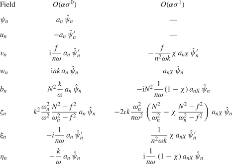
 $\epsilon \ll \sigma$, the polarization relations give expressions for the other fields of interest. These are listed in table 1. Here, the second column gives the usual polarization relations for horizontally periodic disturbances. The last column gives the corrections to these expressions at
 $O(\sigma )$, which are non-zero for a wave packet whose amplitude envelope,
 $a_n$, varies spatially (van den Bremer et al. Reference van den Bremer, Yassin and Sutherland2019). As shown below, including these terms is necessary in the consideration of the induced Eulerian flow with
 $f=0$. However, we will see they can be neglected at leading order in the consideration of the induced Eulerian flow away from the equator.
Expressions for the polarization relations for fields with horizontal wavenumber  $nk$,
 $n=1,2,\ldots$, showing the stream function (
 $\psi _n$), velocity components (
 $u_n$,
 $v_n$,
 $w_n$), buoyancy (
 $b_n$), spanwise vorticity (
 $\zeta _n$),
 $x$-displacement (
 $\xi _n$) and
 $z$-displacement (
 $\eta _n$). The second column shows fields at order
 $\sigma ^{0}$ (corresponding to unmodulated waves) and the third column shows fields at order
 $\sigma ^{1}$. The actual fields are found by adding the
 $O(\sigma ^{0})$ and
 $O(\sigma ^{1})$ terms, multiplying by
 $\alpha (\omega d/k) \exp [\mathrm {i}n(kx-\omega t)]/2$ and adding the complex conjugate. In these expressions, primes on
 $\hat {\psi }$ denote
 $z$-derivatives,
 $a_{nX} \equiv \partial a_n/\partial X$, and
 $\chi \equiv c_g/c_p$ is the ratio of the horizontal group and phase speed of the parent wave.

The expressions for  $u_n$ and
 $w_n$ in table 1 follow directly from (2.7a,b). The expressions for
 $v_n$ and
 $b_n$ are found from the linearized forms of (2.4) and (2.6), The expression for
 $\zeta _n$ follows from the linearized vorticity evolution equation,
 $\zeta _t = - b_x + f v_z$, and using (2.14) to rewrite
 $\hat {\psi }_n^{\prime \prime }$ in terms of
 $\hat {\psi }_n$. Expressions are also given for the horizontal and vertical displacement fields,
 $\xi$ and
 $\eta$, respectively.
2.4. Long wave approximation
In what follows, we will see that the Stokes drift and induced Eulerian flows are a superposition of vertical modes associated with horizontally long disturbances. For this reason, we present the eigenvalue problem for the vertical structure of long waves and the corresponding dispersion relation for different vertical modes. This is presented separately for cases with  $f=0$ and
 $|f|>0$.
In the case  $f=0$, the equation governing the vertical structure,
 $\bar {\psi }_{j}$, of horizontally long, vertical mode-
 $j$ disturbances is given by the solution of the eigenvalue problem
 \begin{equation} \bar{\psi}_{j}^{\prime\prime} ={-}\frac{1}{c_j^{2}} N^{2} \bar{\psi}_{j}, \end{equation}
in which the long wave speed for each mode,  $c_j$, is the eigenvalue. The eigenfunctions, which give the vertical structure of each vertical mode, are orthogonal with respect to the weight
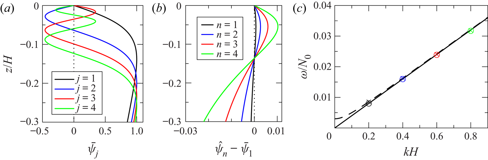
 $N^{2}$. The lowest four modes are plotted in figure 1(a). The corresponding dispersion relation for each vertical mode is
 \begin{equation} \omega^{2} = c_j^{2} k^{2}. \end{equation}
(a) Vertical structure of the lowest four vertical modes of long waves, (b) difference in the vertical structure of the parent wave and first three superharmonics with the mode-1 long wave and (c) dispersion relation for long waves with  $f=0$ (solid black) and
 $f=0.003N_0$ (dashed black), and values of
 $\omega _n(k_n)$ for
 $f=0$ (open circles) and
 $f=0.003N_0$ (crosses). In (a,b) there is no distinguishable differences between plots with
 $f=0$ and
 $f=0.003N_0$.

Away from the equator, the eigenvalue problem for the vertical structure of long disturbances is
 \begin{equation} \bar{\psi}_{j}^{\prime\prime} ={-}\kappa_j^{2}\left(\frac{N^{2}}{f^{2}}-1\right)\bar{\psi}_{j}, \end{equation}
in which  $\kappa _j$ is the eigenvalue. The dispersion relation for each mode is
 \begin{equation} \omega^{2} = f^{2}\left(1 + \frac{k^{2}}{\kappa_j^{2}}\right). \end{equation}
The eigenfunctions,  $\bar {\psi }_j$, are orthogonal with respect to the weight
 $N^{2}-f^{2}$.
If  $|f|\ll N_0=\Vert N\Vert$ in (2.17), the coefficient of
 $\bar {\psi }_j$ on the right-hand side simplifies to
 $-\kappa _j^{2} N^{2}/f^{2}$. Thus, in comparison with (2.15), for both eigenvalue problems we expect the vertical structure of mode-
 $j$ disturbances,
 $\bar {\psi }_j$, to be nearly identical, and we expect the eigenvalues to be related by
 $\kappa _j/f\simeq 1/c_j$ for sufficiently small
 $f$. In particular, for
 $d=0.04H$ we find
 $\kappa _1/f=1/c_1 =25.0/(N_0H)$,
 $\kappa _2/f=1/c_2 =55.8/(N_0H)$ and
 $\kappa _3/f=1/c_3 =86.8/(N_0H)$ for
 $0\leqslant kH\lesssim 0.2$ and
 $0\leqslant f\lesssim 0.003N_0$.
Although the expressions above have been introduced for the purposes of examining the Stokes drift and Eulerian induced flow, the equations with  $j=1$ can also be applied to the mode-1 parent internal tide and its superharmonics, provided the dominant superharmonics are hydrostatic (
 $f\leqslant \omega _n\ll N_0$). As shown in figure 1(b), the difference between the vertical structure, given by (2.14), and the vertical structure of mode-1 long waves, is less than a few per cent for the parent wave and the first three superharmonics. Likewise, figure 1(c) shows that the dispersion relation for mode-1 long waves well represents the frequency of the parent and superharmonics determined by solving (2.14). Thus we can approximate
 $\hat {\psi }_n \simeq \bar {\psi }_1$ for all
 $n$, taking
 $\omega _n^{2} \simeq c_1^{2} (nk)^{2}$ if
 $f=0$, and
 $\omega _n^{2} \simeq f^{2}\,[1+(nk)^{2}/\kappa _1^{2}]$ if
 $|f|>0$.
2.5. Stokes drift
The Stokes drift results from the usual  $O(\alpha ^{2})$ expansion of the mean horizontal velocity arising from horizontally and vertically displaced fluid parcels in varying background flow:
 $\left \langle u\right \rangle _S = \left \langle \xi u_x\right \rangle + \left \langle \eta u_z\right \rangle$, in which angle brackets denote averaging over one wave period.
The leading-order solution does not depend upon the spatial modulation of the amplitude envelope. Using the polarization relations for plane periodic,  $O(\alpha \sigma ^{0})$, internal wave modes, an explicit expression for the Stokes drift due to each of the parent wave (
 $n=1$) and its superharmonics (
 $n>1$) is given in terms of their respective vertical structure functions:
 \begin{equation} \left\langle u_n\right\rangle_S = \frac{1}{4} c_p \,{\rm d}^{2} \alpha^{2} \vert a_n\vert^{2} \frac{{\rm d}^{2}\hat{\psi}_n^{2}}{{\rm d}z^{2}}. \end{equation}
The form of this expression is the same as that found earlier in studies neglecting rotation (Thorpe Reference Thorpe1968; van den Bremer et al. Reference van den Bremer, Yassin and Sutherland2019).
If we assume the parent wave and dominant superharmonics are all hydrostatic, then for all  $n$ we can approximate
 $\hat {\psi }_n\simeq \bar {\psi }_1$, in which
 $\bar {\psi }_1$ is given by the solution of the eigenvalue problem (2.15), if
 $f=0$, and by the solution of (2.17), if
 $|f|>0$. Furthermore, although the parent wave amplitude and its superharmonics vary in time, the sum of the squared amplitudes remains close to unity for all time (Sutherland & Dhaliwal Reference Sutherland and Dhaliwal2022). Consequently, the total Stokes drift,
 $u_S = \sum _n \left \langle u_n\right \rangle _S$ is approximately time-independent, given by
 \begin{equation} u_S = \frac{1}{4} c_p \,{\rm d}^{2} \alpha^{2} \frac{{\rm d}^{2}{\bar{\psi}_1}^{2}}{{\rm d}z^{2}} = \frac{1}{4} c_p A_0^{2} \frac{{\rm d}^{2}{\bar{\psi}_1}^{2}}{{\rm d}z^{2}}. \end{equation}
Unlike the induced superharmonics,  $u_S$ has a mixed mode-1 and mode-2 structure. To demonstrate this, and for comparison with the induced Eulerian flow, which follows, we write the Stokes drift as
 \begin{equation} u_S ={-} c_p \,{\rm d} \alpha^{2} \frac{{\rm d}\varPsi}{{\rm d}z} \quad \mbox{with}\ \varPsi\equiv{-}\frac{{d}}{4}\frac{{\rm d}\bar{\psi}_1^{2}}{{\rm d}z}, \end{equation}
where  $\varPsi$ represents the equivalent of the vertical structure of the stream function associated with the Stokes drift. The modal decomposition of
 $\varPsi$ is given by
 $\varPsi =\sum _j S_j \bar {\psi }_j$, in which the coefficients,
 $S_j$, can be found using the orthogonality of
 $\bar {\psi }_j$ with respect to the weight
 $N^{2}-f^{2}$:
 \begin{align} S_j & = \left[\int (N^{2}-f^{2}) \varPsi \bar{\psi}_j\,{\rm d}z\right] \left[\int (N^{2}-f^{2}) \bar{\psi}_j^{2}\,{\rm d}z\right]^{{-}1} \nonumber\\ & \simeq{-}\frac{d}{2}\left[\int N^{2}\bar{\psi}_1\bar{\psi}_1^{\prime} \bar{\psi}_j\,{\rm d}z\right]\left[\int N^{2}\bar{\psi}_j^{2}\,{\rm d}z\right]^{{-}1}, \end{align}
where the integrals are over the domain depth,  $-H\leqslant z\leqslant 0$. The final expression used the definition of
 $\varPsi$ in (2.21) and made the approximation
 $f\ll \Vert N\Vert = N_0$. Combining these results, we can write the Stokes drift as a superposition of vertical modes according to
 \begin{equation} u_S ={-}c_p \,{\rm d} \alpha^{2} \sum_j S_j \bar{\psi}_j^{\prime}. \end{equation}
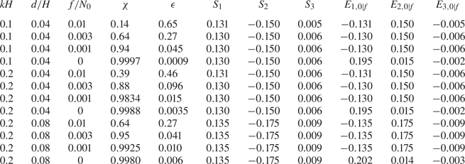
Values of the first three coefficients,  $S_j$, are listed in table 2 for various values of
 $kH$,
 $d/H$ and
 $f_0/N_0$. These show that the values are insensitive to values of the parent wave horizontal wavenumber and Coriolis parameter, provided they are both small. In particular, we see that vertical mode-1 and mode-2 disturbances contribute almost equally to the vertical structure of the Stokes drift with
 $|S_1|\simeq |S_2|\gg |S_3|$.
Values of  $\chi \equiv c_g/c_p$,
 $\epsilon$, eigenvalues for the first three vertical modes, given as
 $N_0H/c_j$ for
 $f=0$ and
 $N_0H\,\kappa _j/f$ for
 $|f|>0$, and nonlinear coupling coefficients (
 $E_{j,0}$ for
 $f=0$ and
 $E_{j,f}$ for
 $|f|>0$).

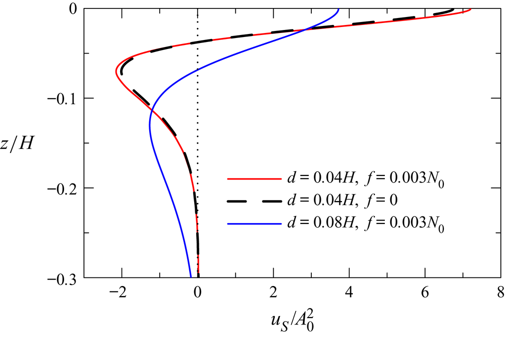
Vertical profiles of the Stokes drift in three circumstances are shown in figure 2. In all cases, the Stokes drift at the surface is oriented in the same direction as the propagation of the parent wave and its superharmonics.
Vertical profiles of the Stokes drift normalized by the squared maximum vertical displacement computed as they are generated by a vertical mode-1 internal tide in exponential stratification with  $d=0.04H$ and
 $0.08H$, and with
 $f=0$ and
 $0.003N_0$, as indicated.

2.6. Induced Eulerian flow
Here we consider the self-interaction of waves resulting in the acceleration of an Eulerian mean flow. The contribution to the forcing of the mean flow by waves of wavenumber  $nk$ is given by substituting into (2.10) the expressions for velocity, buoyancy and vorticity using the polarization relations listed in table 1. Extracting the cross-terms in the products of fields with their complex conjugates gives expressions not involving the complex exponentials. Thus we find
 \begin{align} \left\langle \boldsymbol{\nabla}\boldsymbol{\cdot}\boldsymbol{F}_n\right\rangle & = \frac{1}{2} \frac{\omega}{k} \frac{{\rm d}^{2}\alpha^{2}}{\omega_n^{2}-f^{2}} \left\{\vphantom{\left[4\left(N^{2}-\omega_n^{2}\right) \hat{\psi}_n \hat{\psi}_n^{\prime} + \frac{{\rm d}N^{2}}{{\rm d}z} \hat{\psi}_n^{2} \right]} \sigma^{2}\left[\vphantom{\left[4\left(N^{2}-\omega_n^{2}\right) \hat{\psi}_n \hat{\psi}_n^{\prime} + \frac{{\rm d}N^{2}}{{\rm d}z} \hat{\psi}_n^{2} \right]}(1+2\chi)\left((1-\chi)N^{2}\omega_n^{2} -f^{2}(N^{2} - \chi^{2}\omega_n^{2})\right) \hat{\psi}_n \hat{\psi}_n^{\prime}\right.\right. \nonumber\\ & \quad\left. -\frac{\chi}{2}\left(2\chi\omega_n^{2} + f^{2}\right)\frac{{\rm d}N^{2}}{{\rm d}z}\hat{\psi}_n^{2} \right]\partial_{XX}|a_n|^{2} \nonumber\\ & \quad -\epsilon\sigma\frac{k}{\omega} \left[\vphantom{\left[4\left(N^{2}-\omega_n^{2}\right) \hat{\psi}_n \hat{\psi}_n^{\prime} + \frac{{\rm d}N^{2}}{{\rm d}z} \hat{\psi}_n^{2} \right]}2\left((1-\chi)N^{2}\omega_n^{2} -f^{2} (N^{2} - \chi \omega_n^{2})\right) \hat{\psi}_n \hat{\psi}_n^{\prime}\right. \nonumber\\ & \left.\quad+\frac{1}{2}\left((2\chi-1)\omega_n^{2} + 2f^{2}\right)\frac{{\rm d}N^{2}}{{\rm d}z}\hat{\psi}_n^{2} \right]\partial_{TX}|a_n|^{2} \nonumber\\ & \quad \left. -f^{2} \left[4\left(N^{2}-\omega_n^{2}\right) \hat{\psi}_n \hat{\psi}_n^{\prime} + \frac{{\rm d}N^{2}}{{\rm d}z} \hat{\psi}_n^{2} \right] \left((nk)^{2}|a_n|^{2} - \chi |\partial_X a_n|^{2}\right) \right\}. \end{align}
In considering the response to this nonlinear forcing, we seek the stream function,  $\psi ^{(0)}$, satisfying
 $\mathcal {L}\psi ^{(0)} = \sum _n\left \langle \boldsymbol {\nabla }\boldsymbol {{\cdot }}\boldsymbol {F}_n\right \rangle$, in which
 $\mathcal {L}$ is given by (2.9). In the case of superharmonic excitation, the near-resonance of the parent with superharmonics results in the dominant excitation of a vertical mode-1 disturbance. This is not necessarily the case for the forcing of the induced Eulerian flow. Consequently, the stream function for this induced flow is written as a superposition of vertical modes:
 \begin{equation} \psi^{(0)} = \frac{\omega d}{k} \alpha^{2} \sum_j A_{j}(X,T) \bar{\psi}_{j}(z), \end{equation}
in which  $j=1,2,\ldots$ is the vertical mode number.
Using (2.9) and (2.25), we find
 \begin{align} {\mathcal{L}}\psi^{(0)} &= \alpha^{2} \frac{\omega d}{k} \sum_j \left[ \sigma^{2} \left( \epsilon^{2} \partial_{XXTT} A_{j} - 2\epsilon\sigma c_g \partial_{XXXT} A_{j} +\sigma^{2} c_g^{2} \partial_{XXXX} A_{j}\right) \bar{\psi}_{j} \right. \nonumber\\ & \quad + \left(\epsilon^{2} \partial_{TT} A_{j} - 2\epsilon\sigma c_g \partial_{XT} A_{j} +\sigma^{2} c_g^{2} \partial_{XX} A_{j}\right) \bar{\psi}_{j}^{\prime\prime} \nonumber\\ & \left. \quad+\sigma^{2} N^{2} \left(\partial_{XX} A_{j}\right)\bar{\psi}_{j} + f^{2}\, A_{j}\,\bar{\psi}_{j}^{\prime\prime} \right]. \end{align}
The form of the forcing (2.24) and the linear response (2.26) simplify considerably if we make use of the long wave approximation for  $\bar {\psi }_j$ given by (2.15), if
 $f=0$, and by (2.17), if
 $|f|>0$. This suggests the need to consider these two cases separately, as done in the following two subsections.
2.6.1. Case with  $f=0$

Previous work (van den Bremer et al. Reference van den Bremer, Yassin and Sutherland2019) considered steady-state solutions for the Eulerian flow induced by the parent wave alone in a background with no rotation. By examining the special case of piecewise-constant  $N^{2}$ profiles, they found that the dominant structure of the induced flow was a vertical mode-1 disturbance, provided that
 $N^{2}$ was not symmetric about the mid-depth. At the surface this flow was opposite to and dominated over the Stokes drift. By using the vertical mode decomposition of
 $\psi ^{(0)}$ given by (2.25), the symmetry breaking of the vertical structure is derived for arbitrary
 $N^{2}$ profiles in Appendix A. In contrast to studies of steady-state induced flows, here we show that the transiently induced Eulerian flow is not dominated by a mode-1 structure, nor is it dominant over the Stokes drift. Indeed, for periodic waves the induced Eulerian flow is negligibly small compared with the Stokes drift. However, for horizontally modulated waves the Eulerian flow can grow non-uniformly in time and space to become comparable to the Stokes drift.
The expressions for the nonlinear forcing (2.24) and the linear response (2.26), can be simplified using the long wave approximations for  $f=0$, given by the eigenvalue problem (2.15) and (2.16). In particular, we take
 $\omega _n^{2} \simeq c_1^{2} (nk)^{2}$ and
 $\hat {\psi }_n\simeq \bar {\psi }_1$. Owing to the long wave linear dispersion relation in (2.15), the group and phase velocities are equal. Likewise, for the parent internal tide, we have
 $c_g\simeq c_p \simeq c_1$. Hence
 $\chi \equiv c_g/c_p\simeq 1$. At the equator,
 $\epsilon$ is very small owing to the near-linearity of the dispersion relation. Thus we may take
 $\epsilon \ll \sigma$, and the nonlinear forcing by the parent wave and each superharmonic simplifies to
 \begin{equation} \left\langle\boldsymbol{\nabla}\boldsymbol{\cdot} \boldsymbol{F}_n\right\rangle \simeq{-}\frac{1}{2} \frac{\omega}{k}{\rm d}^{2} \alpha^{2} \sigma^{2} \frac{{\rm d}N^{2}}{{\rm d}z} \bar{\psi}_{1}^{2} \partial_{XX}|a_n|^{2}. \end{equation}
In the linear response operator we set  $f=0$ and retain only the terms at
 $O(\sigma ^{2})$ and
 $O(\sigma \epsilon )$, the latter being kept so that we have a time evolution equation for
 $A_{j}$. Using (2.15) to replace terms involving
 $\bar {\psi }_j^{\prime \prime }$ in
 $\mathcal {L}\psi ^{(0)}$ with terms involving
 $\bar {\psi }_j$, we find
 \begin{equation} \mathcal{L}\psi^{(0)} \simeq \alpha^{2} \frac{\omega d}{k} N^{2} \sum_j\, \bar{\psi}_{j} \left[ 2 \frac{c_1}{c_j^{2}} \sigma \epsilon \partial_{XT} A_{j} + \left(1-\frac{c_1^{2}}{c_j^{2}}\right)\sigma^{2} \partial_{XX} A_{j} \right]. \end{equation}
We equate (2.28) to the sum over  $n$ of the forcing given by (2.27) and integrate both sides by
 $X$. Making use of the orthogonality of
 $\bar {\psi }_j$ with respect to weight
 $N^{2}$, we multiply both sides by
 $\bar {\psi }_j$ and integrate in
 $z$ to give the resulting time-evolution equation for
 $A_j$:
 \begin{equation} \partial_T A_j + \frac{1}{2}\frac{\sigma}{\epsilon}\left(\frac{c_j^{2}}{c_1^{2}}-1\right) c_1 \partial_X A_j \simeq{-} c_1 \frac{\sigma}{\epsilon} E_{j,0}\,\partial_X \left[ \sum_n |a_n|^{2} \right]. \end{equation}
Here we used  $c_g\simeq c_p \simeq c_1$, and we defined the interaction coefficient
 $E_{j,0}$ by
 \begin{equation} E_{j,0} \equiv \frac{1}{4} d \frac{c_j^{2}}{c_1^{2}} \left[ \int \frac{{\rm d}N^{2}}{{\rm d}z} \bar{\psi}_1^{2} \bar{\psi}_j \,{\rm d}z \right]\left[\int N^{2} \bar{\psi}_{j}^{2}\,{\rm d}z\right]^{{-}1}. \end{equation}
Values of the lowest three interaction coefficients are given in table 2.
Explicit solutions for (2.29) can be found by noting that the sum of the squared amplitudes of the parent wave and superharmonics remains approximately constant in time (Sutherland & Dhaliwal Reference Sutherland and Dhaliwal2022, Appendix B). Hence the sum in (2.29) is approximately equal to the initial parent wave squared amplitude  $|a_1(X,0)|^{2}$. Defining the change of variables
 $\tilde {T}=T\equiv \epsilon t$ and
 $\tilde {X}= X-(\sigma /\epsilon )c_1(\gamma _j-1) T = \sigma (x-c_1\gamma _j t)$, in which
 $\gamma _j \equiv (1+c_j^{2}/c_1^{2})/2$, (2.29) becomes
 $\partial _{\tilde {T}} A_j = -({\sigma }/{\epsilon }) c_1 E_{j,0} \partial _{\tilde {X}}|a_1(\tilde {X},0)|^{2}$. The solution cast in terms of fast time and space variables is
 \begin{equation} A_j(x,t) ={-} c_1 E_{j,0}\kern1.5pt t\kern1.5pt \partial_x |a_1(\sigma(x-c_1\gamma_j\kern1.5pt t\kern1.5pt),0)|^{2}. \end{equation}
The explicit formula for the induced Eulerian flow is
 \begin{equation} u_E(x,z,t) = \alpha^{2} c_1^{2} \,{\rm d}\kern0.06em t\sum_j E_{j,0} \partial_x |a_1(\sigma(x-c_1\gamma_j\kern1.5pt t\kern1.5pt),0)|^{2} \bar{\psi}_j^{\prime} . \end{equation}
This shows that the horizontally averaged induced flow, is zero for a modulated disturbance that is compact or periodic in  $x$. Nonetheless, at any horizontal location, the vertical profile of the Eulerian induced flow can exhibit a complex time-evolving structure due to the varying propagation speeds set by
 $\gamma _j$, which depends upon the horizontal phase speeds,
 $c_j$, of each vertical mode. For the lowest vertical mode,
 $\gamma _1=1$, and
 $\gamma _j\rightarrow 1/2$ for
 $j\gg 1$. Although (2.31) predicts a linear growth in time of each vertical mode, the fully nonlinear simulations, which follow, demonstrate that the growth eventually becomes retarded. This we attribute to Doppler shifting of the waves by the Eulerian induced flow.
Because the Stokes drift is  $O(\sigma ^{0})$, the Lagrangian transport for waves near the equator is initially dominated by the Stokes drift. Assuming
 $|E_{1,0}|\sim |S_1|$, the magnitude of the induced Eulerian flow associated with mode-
 $1$ disturbances becomes comparable to the Stokes drift after a time of the order
 $\omega ^{-1}/(\alpha _{{\small mod}}\sigma )$, in which
 $\alpha _{{\small mod}}$ denotes the relative amplitude of the modulation and
 $\sigma$ represents the horizontal scale of the waves to the horizontal scale of the modulations.
As an example, we consider a modulated parent internal tide with initial maximum vertical displacement given by (2.2). In this case
 \begin{equation} a_1(x,0) = 1 + \alpha_{{\small mod}} \cos(Kx), \end{equation}
with  $\alpha _{{\small mod}}\equiv {A_{{\small mod}}}/A_0$ and
 $K=\sigma k$. Using parameters based on the Farfield observations south-west of Hawaii, we take
 $kH=0.2$,
 $A_0\simeq 0.003H$,
 ${A_{{\small mod}}}=0.002H$ and
 $\sigma =1/16$. The background stratification is given by (2.1) with
 $d=0.04H$ and
 $z_0=-0.019H$. For these parameters,
 $c_1\simeq 0.04 N_0 H$ and
 $\omega _1\simeq 0.008N_0$. Hence, the induced Eulerian flow associated with mode-1 disturbances is expected to become comparable to the Stokes drift at times
 $N_0t\simeq 3000$, corresponding to approximately two days given
 $N_0\simeq 0.017~\mbox {s}^{-1}$.
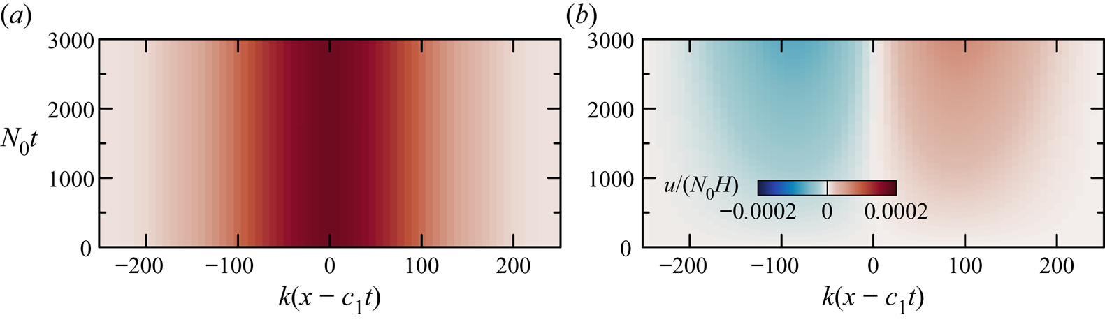
The Stokes drift associated with this modulated wave is given by (2.20) after multiplying by  $|a_1(x-c_1 t,0)|^{2}$. The evolution of the surface expression of the Stokes drift is plotted in figure 3(a). In a frame moving with the group velocity,
 $u_S$ does not vary in time.
Horizontal time series at  $z=0$ in a frame moving with the group velocity of the parent wave,
 $c_g=c_1$, of (a) the Stokes drift and (b) the Eulerian induced flow for a periodically modulated internal tide with
 $\alpha _{{\small mod}}=2/3$ and
 $\sigma =1/16$ in exponential background stratification with
 $d=0.04H$ and
 $z_0=-0.019H$, and with no background rotation (
 $f=0$). The velocity scale for both plots is shown in (b).

The surface expression of  $u_E$, calculated using (2.32) and (2.33), is plotted in figure 3(b). This shows the slow growth in time of
 $u_E$, being opposite signed about the maximum of the amplitude envelope at early times but drifting rightwards relative to the group velocity as the disturbances grow in time.
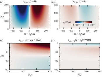
The rightward drift can be explained by considering the superposition of the Eulerian induced flow associated with each vertical mode. Horizontal time series of the surface expression of the induced flow for the lowest two vertical modes is shown in figure 4(a,b). Because  $E_{1,0}$ is the largest of the interaction coefficients, this mode grows most quickly. However, because
 $\gamma _1=0$, there is no lateral drift associated with the vertical mode-1 flow. In contrast, although the higher vertical modes grow more slowly, their surface signal drifts leftward because
 $\gamma _j>0$ for
 $j>1$. The sign of the induced Eulerian flow for vertical mode
 $j=2$ at the surface is oppositely signed to the mode-1 Eulerian flow. Consequently, the superposition of the vertical modes results in an increasing negative surface flow at
 $x-c_1t=0$.
For the modulated tide considered in figure 3, time series of the breakdown of the Eulerian flow into the lowest two vertical modes (a,c)  $j=1$, (b,d)
 $j=2$ showing (a,b) the horizontal time series at
 $z=0$ and (c,d) the vertical time series at
 $x-c_1 t = 90H$. The velocity scale in all plots is shown in (b).

The decomposition of the vertical structure of the flow into its constituent vertical modes is shown in figure 4(c,d). These time series are extracted from vertical profiles of the flow at  $x-c_1t \simeq 90H$, corresponding approximately to the location of the peak magnitude of the forcing of the Eulerian induced flow. As noted above, the surface expression of the induced Eulerian flow is weaker than that at depth because the flow associated with the vertical mode-1 disturbance destructively interferes with the flow associated with the mode-2 disturbance at
 $z=0$. The modes interfere constructively at depths around
 $z\simeq -0.05H$ leading to a net rightward flow to the right of the peak of the modulated amplitude envelope of the primary wave.
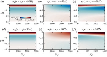
The evolution of the vertical profiles of the Stokes drift, induced Eulerian flow and the Lagrangian flow at  $x-c_1t=\pm 90H$ are shown in figure 5. At both locations, the Stokes drift dominates over the induced Eulerian flow at the surface over the times shown. In the lee of the peak in the modulated amplitude envelope, the Eulerian induced flow is negative above
 $z\simeq -0.15H$ and grows in magnitude over time. This results in a narrowing depth of the rightward Lagrangian transport near the surface with a time-increasing leftward flow at a depth around
 $z\simeq -0.05H$. At greater depth,
 $z\lesssim -0.2H$, the Lagrangian transport is rightward once more, being dominated by the induced Eulerian flow. Leading the peak of the modulated amplitude envelope, the Stokes drift and induced Eulerian flow are both rightward leading to a deepening of the vertical extent of the rightward Lagrangian transport with weak leftward motion below.
Vertical time series of (a,d) the Stokes drift, (b,e) the Eulerian induced flow and (c,f) the Lagrangian flow taken at (a–c)  $x-c_1 t=-90H$ and (d–f)
 $x-c_1 t = 90H$. The internal tide parameters are same as those in figure 3.

2.6.2. Case with $|f| > 0$

With  $f$ non-zero, the leading-order forcing terms in (2.24) are
 $O(\epsilon ^{0}\sigma ^{0})$. Hence we can assume to leading order that the parent wave is horizontally periodic so that
 $a_1(x,0)=1$ and
 $A_j=A_j(T)$ with
 $A_j(0)=0$ for
 $j=1,2,\ldots$ . These terms may be further simplified making use of (2.18) and assuming that
 $\omega _n\ll N_0$. Thus we find
 \begin{equation} \left\langle\boldsymbol{\nabla}\boldsymbol{\cdot}\boldsymbol{F}_n\right\rangle \simeq{-}\frac{1}{2} \frac{\omega}{k} {\rm d}^{2} \kappa_1^{2} \alpha^{2} \left[4 N^{2} \bar{\psi}_1\bar{\psi}_1^{\prime} + \frac{{\rm d}N^{2}}{{\rm d}z}\bar{\psi}_1^{2}\right]|a_n|^{2}. \end{equation}
As for the linear response given generally by (2.26), because  $\sigma \ll \epsilon$ away from the equator, we only keep the
 $O(\,f/N_0)$ and
 $O(\epsilon ^{2})$ terms, and we make use of (2.17):
 \begin{equation} \mathcal{L}\psi^{(0)} \simeq{-}\alpha^{2} \frac{\omega d}{k} \frac{N^{2}-f^{2}}{f^{2}} \sum_j \kappa_j^{2} \left( \epsilon^{2} \partial_{TT} A_j + f^{2} A_j \right) \bar{\psi}_j .\end{equation}
Equating this to the sum of the forcing terms in (2.34), then multiplying both sides by  $\bar {\psi }_j$ and integrating with respect to
 $z$ gives
 \begin{equation} \partial_{TT}A_j + (\,f/\epsilon)^{2} A_j \simeq (\,f/\epsilon)^{2} E_{j,f} \sum_n |a_n|^{2}, \end{equation}
in which
 \begin{equation} E_{j,f} \simeq \frac{1}{2} d \frac{\kappa_1^{2}}{\kappa_j^{2}} \left[ \int 4 N^{2} \bar{\psi}_1 \bar{\psi}_1^{\prime} \bar{\psi}_{j} + \frac{{\rm d}N^{2}}{{\rm d}z} \bar{\psi}_1^{2} \bar{\psi}_{j}\,{\rm d}z \right] \left[\int N^{2}\bar{\psi}_{j}^{2}\,{\rm d}z\right]^{{-}1}, \end{equation}
where we have assumed  $|f|\ll \Vert N\Vert =N_0$ in the integrand of the last expression. The expressions for
 $E_{j,f}$ in (2.37) and
 $S_j$ in (2.22) look quite different. However, as shown in Appendix B, for long waves their values are equal and opposite. This is also clear by comparing the tabulated values of
 $E_{j,f}$ and
 $S_j$ for
 $|f|>0$ in table 2. Hence, with
 $|f|>0$, the vertical structure of the induced Eulerian flow is equal and opposite to the vertical structure of the Stokes drift.
Because 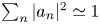 $\sum _n|a_n|^{2}\simeq 1$ for all time (Sutherland & Dhaliwal Reference Sutherland and Dhaliwal2022), we can immediately find the solution of (2.37) for each vertical mode using
 $T=\epsilon t$ to express the result in the fast-time variable,
 $t$:
 \begin{equation} A_j(t) \simeq E_{j,f} \left(1-\cos(\,ft)\right). \end{equation}
The induced Eulerian flow is thus given approximately by
 \begin{equation} u_E ={-}c_p \,{\rm d} \alpha^{2} \left[\sum_j E_{j,f} \bar{\psi}_j^{\prime}\right] \left(1-\cos(\,ft)\right). \end{equation}
In particular, for long waves on the  $f$-plane, we can use (2.23) with
 $S_j \simeq -E_{j,f}$, in which case we have
 \begin{equation} u_E \simeq{-} u_S \left(1-\cos(\,ft)\right). \end{equation}
Unlike the case with  $f=0$, the induced Eulerian flow oscillates at the inertial period and all vertical modes vary equally in time. The occurrence of inertial oscillations in response to the Stokes drift of surface waves influenced by Coriolis forces was originally predicted by Hasselmann (Reference Hasselmann1970) (see also Onink et al. Reference Onink, Wichmann, Delandmeter and van Sebille2019; Higgins, Vanneste & van den Bremer Reference Higgins, Vanneste and van den Bremer2020). Here this result for the internal tide was derived through an alternate approach, relying on the long wave approximation on the
 $f$-plane giving
 $S_j\simeq -E_{j,f}$ (Appendix B). This relationship does not hold for more non-hydrostatic waves on the
 $f$-plane, in which case the general expression for
 $u_E$ given by (2.39) should be used with
 $E_{j,f}$ given by (2.37).
Figure 6 shows the prediction for the Stokes drift and the induced Eulerian and Lagrangian flows in the case of a parent wave with  $kH=0.2$,
 $A_0=0.003H$ and
 $f=0.003N_0$. The corresponding inertial period is
 $2{\rm \pi} /f \simeq 2094 N_0^{-1}$. Stratification is given by (2.1) with
 $d=0.04H$ and
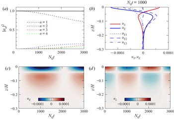
 $z_0=-0.019H$. The evolution of the squared amplitude of the parent wave and its superharmonics is shown in figure 6(a). Although the amplitude of the parent wave decreases in time at the expense of the growth of superharmonics, the sum of the squared amplitudes remains constant, consistent with the assumption of the theory. Vertical profiles of the Stokes drift and the induced Eulerian flow at
 $N_0t=1000$ (corresponding approximately to half an inertial period) are shown in figure 6(b), together with the breakdown of the induced Eulerian flow into the first three vertical modes. The Eulerian flow is negative at the surface, whose magnitude at half an inertial period is nearly double the magnitude of the Stokes drift. Thus, when superimposed with the steady Stokes drift, the resulting Lagrangian flow oscillates between positive and negative values over one inertial period (figure 6d). As a consequence of the relationship between the induced Eulerian flow and Stokes drift given by (2.39), the average Lagrangian transport over one inertial period is zero.
For  $f=0.003N_0$ and
 $A_0=0.003$, (a) the predicted time evolution of the squared amplitudes of the parent wave (
 $n=1$), its first three superharmonics (
 $n=2,3,4$), and the sum of the squared amplitudes (thick solid line), (b) vertical structure of the Stokes drift (
 $u_S$) and, at
 $N_0t=1000$, the induced Eulerian flow (
 $u_E$) with its decomposition into the first three vertical modes (
 $u_{E1}$,
 $u_{E2}$,
 $u_{E3}$), (c) vertical time series of the predicted induced Eulerian flow and (d) vertical time series of the predicted Lagrangian flow,
 $u_L=u_E+u_S$. For these results, the background stratification is assumed to be exponential with
 $d=0.04H$ and
 $z_0=-0.019H$, the Coriolis parameter is
 $f=0.003N_0$, and the parent mode-1 internal tide has
 $kH=0.2$ and
 $A_0=0.003H$.

3. Numerical solutions
3.1. Fully nonlinear simulations
The fully nonlinear equations are solved using the same code described in the companion paper (Sutherland & Dhaliwal Reference Sutherland and Dhaliwal2022). The two-dimensional rotating Boussinesq equations are solved in a rectangular domain with horizontally periodic boundary conditions and free-slip conditions at the top and bottom of the domain. Explicitly, the evolution equations are solved for the spanwise vorticity,  $\zeta$, spanwise velocity,
 $v$, and buoyancy,
 $b$. The (spanwise) stream function,
 $\psi$, is solved by inverting the Laplacian equation
 $\nabla ^{2}\psi = -\zeta$ and, from this, we find the
 $x$- and
 $z$-components of the velocity field. The equations are solved by representing the
 $x$-components of the fields in Fourier space, and finite-differences are used to take derivatives in the vertical direction. In the vertical, fields are discretized by
 $257$ evenly spaced points. In the horizontal, the spectral fields are resolved by
 $128$ wavenumbers for each wavenumber of the parent internal tide. In simulations of the modulated internal tide, the horizontal extent of the domain is resolved by
 $2048$ horizontal wavenumbers. Momentum and substance diffusion are included for numerical stability using Laplacian diffusion acting only upon horizontal wavenumbers larger than
 $32k$.
In all simulations presented here, the background stratification is taken to be exponential, given by (2.1) with  $d=0.04H$ and
 $z_0=-0.019H$. For prescribed horizontal wavenumber, taken to be
 $k=0.2H^{-1}$, the vertical structure and frequency of the mode-1 wave is computed numerically. These are used to determine the initial fluctuation fields associated with the waves. The waves are prescribed to be either horizontally periodic or horizontally modulated. Explicitly, the stream function for the waves is given by
 $\psi (x,z,t=0) = A_0(\omega /k) a(X)\,\hat {\psi }_1(z) \cos (kx)$, in which
 $A_0=0.003H$. For periodic waves we set
 $a(X)=1$, and for modulated waves we set
 $a(X) = 1 + \alpha _{{\small mod}}\cos (Kx)$, in which
 $\alpha _{{\small mod}}=0.67$ and
 $K=k/16$.
In order to assess Lagrangian transport, an additional equation is solved to determine the horizontal,  $\xi$, and vertical,
 $\eta$, parcel displacements resulting from advection,
 \begin{equation} \partial_t (\xi,\eta) ={-} u \partial_x(\xi,\eta) - w \partial_z(\xi,\eta), \end{equation}
for which, initially,  $\xi (x,z,t=0)= \alpha ({d}/{k}) a_1(X,0) \hat {\psi }_1^{\prime } \sin (kx-\omega t)$ and
 $\eta (x,z,t=0)= -\alpha \,{\rm d} a_1(X,0) \hat {\psi }_1 \cos (kx-\omega t)$ (see table 1). In (3.1),
 $(u,w)$ is evaluated in real space at the location of the displaced parcel at
 $(x+\xi,z+\eta )$ using bilinear interpolation.
For horizontally periodic parent internal waves, the horizontal induced Eulerian flow is given by  $u_E = \left \langle u\right \rangle$ and the horizontal Lagrangian transport is given by
 $\left \langle \xi _t\right \rangle$, in which the angle brackets denote averaging over the horizontal domain. For horizontally modulated parent waves, the Eulerian flow is found by applying a low-pass Fourier filter, keeping only those modes with horizontal wavenumbers less than
 $4K$.
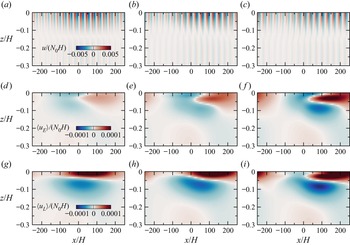
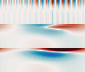
We start by considering the results of a simulation of a periodically modulated wave with  $f=0$. The horizontal velocity field computed from this simulation is shown at three times in figure 7(a–c). As in Sutherland & Dhaliwal (Reference Sutherland and Dhaliwal2022), this reveals the formation of solitary internal wave packets, being most pronounced where the amplitude of the modulated wave is large. Despite this horizontal transformation of the wave structure over a wavelength of the primary wave, the squared amplitude envelope of the disturbance remains unchanged except for its rightward translation at the group velocity,
 $c_g\simeq c_1$. It is the evolution of the squared amplitude envelope, and not the waves within, that dominate the evolution of the Stokes drift, induced Eulerian flow and the Lagrangian flow.
Simulation results at times (a,d,g)  $N_0t=1000$, (b,e,h)
 $N_0t=2000$ and (c,f,i)
 $N_0t=3000$ showing the (a–c) the instantaneous horizontal velocity, (d–f) the low-pass filtered horizontal velocity and (g–i) the low-pass filtered Lagrangian flow. In all cases
 $f=0$, the background stratification is given by (2.1) with
 $d=0.04H$ and
 $z_0=-0.019H$, and the initial parent internal tide has wavenumber
 $kH=0.2$, modulated according to (2.2) with
 $A_0=0.003H$,
 ${A_{{\small mod}}}=0.002H$ and
 $K=k/16$. The horizontal velocity scales in (a,d,f) correspond to the plots in successive columns of the figure.

The mean Eulerian flow (figure 7d–f) exhibits the time-evolving structure predicted by theory. Its magnitude increases in time, with increasing leftward flow at the surface to the right of the translating peak of the amplitude envelope, and increasing rightward flow at a depth around  $0.04H$. The Lagrangian flow is dominated by the Stokes drift at early times, being near-constant in time and positive at the surface. Consistent with theory, the induced Eulerian flow grows linearly at early times with higher vertical modes advancing at progressively smaller speeds. Its superposition with the Stokes drift leads to a complex time-evolving structure of the Lagrangian flow. At late times, this flow reverses direction near the surface in the lee of the peak of the modulated wave packet while the subsurface rightward flow intensifies below the peak (figure 7g–i).
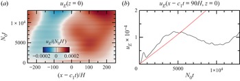
The time evolution of the surface flow is examined in figure 8. This flow is shown in a frame of reference moving with the predicted horizontal group velocity of the parent wave  $c_g=c_1$. Here it is apparent that there are fluctuations in this flow occurring on a time scale of order
 $500/N_0$ which are superimposed on an initially steady growth of the induced flow up to time
 $N_0t\simeq 5000$ (figure 8a). This is followed by a moderate reduction in the induced flow before it increases again. Focusing on the time-evolution of the flow at
 $x-c_1 t=90H$, we see that the growth up to
 $N_0t=4000$ is approximately linear with growth rate moderately larger than that predicted by the theory (figure 8b). Whereas the theory predicts continuing linear growth beyond this time, according to (2.32), the simulations show a temporary reduction in the amplitude before growing again. The deviation from the theory, both in terms of the fluctuations and the decrease in the induced Eulerian flow after
 $N_0t\simeq 5000$ is attributed to the action of the induced Eulerian flow upon the waves, which Doppler shifts the waves differentially with depth, so changing their vertical structure. While interesting in theory, examination of these dynamics lies beyond the scope of this work.
For the simulation shown in figure 7, (a) horizontal time series of the induced Eulerian flow at  $z=0$ shown in a frame of reference moving at the horizontal group velocity and (b) the evolution of this flow at
 $x-c_1 t=90H$ (black line) compared with the prediction of theory (red line).

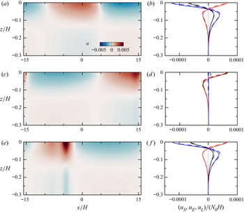
Simulations examining the evolution of the parent wave on the  $f$-plane is compared with theory in figure 9. Here the parent wave is taken to be horizontally periodic with amplitude
 $A_0=0.003H$. As shown by Sutherland & Dhaliwal (Reference Sutherland and Dhaliwal2022), the superharmonic cascade results in the generation of internal solitary waves. Despite the modification of the wave structure, the sum of the amplitude-squared forcing by the parent and superharmonic waves remains constant. Consequently, the theoretical prediction for the Stokes drift and the induced Eulerian flow is well represented by theory given by (2.20) and (2.39), respectively. Specifically, the Stokes drift remains steady in time, while the induced Eulerian flow oscillates at the inertial period, alternately changing the sign of the Lagrangian flow between rightward and leftward with respect to the direction of parent wave propagation.
Simulation results for an initially horizontally periodic internal tide in rotating fluid with  $f=0.003N_0$ at times (a)
 $N_0t=1000$, (c)
 $N_0t=2000$ and (e)
 $N_0t=3000$ showing (a,c,e) the horizontal velocity field and (b,d,f) the horizontally averaged horizontal velocity (dashed blue), Stokes drift (dashed red) and Lagrangian velocity (dashed black). The horizontally averaged simulated flows are compared in (b,d,f) with the theoretically predicted induced Eulerian flow (solid blue), Stokes drift (solid red) and Lagrangian flow (solid black). In all cases the background stratification is given by (2.1) with
 $d=0.04H$ and
 $z_0=-0.019H$, and the initial parent internal tide has wavenumber
 $kH=0.2$.

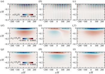
For comparison with the simulation of a modulated wave packet with  $f=0$ (figure 7), in figure 10 we also show snapshots of the horizontal velocity, the induced Eulerian flow and the Lagrangian flow computed from a simulation of the modulated wave packet with
 $f=0.003N_0$. As anticipated, this shows that the Stokes drift and Eulerian flow have largest magnitude where the amplitude envelope of the modulated waves is largest. At the times where the induced Eulerian flow is strongest (
 $N_0t\simeq 1000$ and
 $3000$), it dominates over the Stokes drift resulting in negative Lagrangian transport near the surface. After an inertial period (
 $N_0t\simeq 2000$), the Eulerian flow is weakest and the Stokes drift dominates, resulting in a positive Lagrangian transport at the surface. The results are thus consistent with the predicted and simulated behaviour of horizontally periodic waves (figure 9), with the amplitude envelope modulation simply resulting in a corresponding spatial modulation of the Eulerian flow, Stokes drift and Lagrangian transport.
As in figure 7 but for a simulation of a horizontally modulated wave packet with  $f=0.003N_0$.

4. Conclusions
The self-interaction of internal tides results in the forcing of an induced Eulerian flow. Although the internal tide can transform into a solitary wave train as a consequence of excitation of superharmonics, the sum of the forcing due to the primary wave and its superharmonics remains nearly constant in time. The evolution and structure of the mean flow response to this forcing depends upon the influence, or not, of Coriolis effects.
In the presence of Coriolis forces ( $|f|>0$), the forcing acts equally upon all vertical modes in the decomposition of the induced Eulerian flow. This flow responds through inertial oscillations at frequency
 $f$ with predominantly negative flow at the surface reaching a peak that is opposite to and nearly double the time-independent Stokes drift at the surface. Consequently, the superposition of the Stokes drift and induced Eulerian flow gives a Lagrangian transport that oscillates between positive and negative in time, with zero net transport over one inertial period.
If  $f=0$, the induced Eulerian flow is negligible with respect to the Stokes drift for horizontally periodic waves. This prediction lies in contrast with the theory for the steady (time-invariant in a frame moving with the group velocity of the internal tide) induced Eulerian flow, which predicts the excitation of a relatively strong flow with mode-1 structure. Such steady flows are unlikely to be manifest in practice. For horizontally modulated internal tides, oppositely signed induced Eulerian flows are excited on either side of the peak in the modulation which initially grows linearly in time. While the component of the induced Eulerian flow that has vertical mode-1 structure translates with the group velocity of the internal tide as it grows, higher modes propagate at different speeds leading to a complex vertical structure in space and time. In reality, of course, at the equator the waves would be influenced by the quasi-steady zonal currents manifest there. And so, while interesting in theory to consider the Lagrangian transport by internal tides where
 $f=0$, in practice zonal flows would dominate transport. Nonetheless, the spatiotemporally evolving complex structure of the induced Eulerian flow as the internal tide nears the equator, could influence the vertical structure of the equatorial currents.
In the context of the influence of the internal tide upon mass transport, we have seen that their Lagrangian transport by internal tides is negligible when averaged over an inertial period on the  $f$-plane or when averaged horizontally over the spatial scale of amplitude modulations. Instantaneously, the magnitude of the Lagrangian flow is of the order of
 $c_p \alpha ^{2}$ which, for observed values near Hawaii, is approximately
 $0.03~\mbox {m}~\mbox {s}^{-1}$. Although insignificant near the surface, the transport persists at depths hundreds of metres below the surface where the influence of the Stokes drift due to surface waves is negligible.
The theory makes several approximations that limit its application to realistic internal tides. As well as assuming constant-depth fluid, the waves are assumed to be spanwise invariant. Preliminary three-dimensional numerical simulations on the  $f$-plane examining the evolution of a periodic internal tide with finite spanwise extent show its evolution is qualitatively similar to spanwise invariant waves in that superharmonics are excited along the centre of the beam and the Eulerian induced flow oscillates at the inertial periodic across the lateral extent of the beam. Ongoing research aims to develop quantitative predictions for the observed flows. The work presented here is also limited to the initial value problem in which a modulated tide is prescribed on the
 $f$-plane. Ongoing work is extending this study to examine a tide that is forced near the left-hand side of the domain and propagates rightward on the beta-plane towards decreasing
 $f$. We have also neglected the influence of the barotropic mode associated with the waves (Dong et al. Reference Dong, Bühler and Smith2020). Interactions with currents and eddies have also been neglected. A complete understanding for mass transport influenced by internal tides should additionally account for depth variations and effects associated with ocean currents and eddies.
Funding
This research was funded in part by the Natural Sciences and Engineering Research Council (NSERC) of Canada. Simulations were made possible through a resource allocation from Compute Canada applied to the supercomputers ‘graham’ and ‘cedar’.
Declaration of interests
The authors report no conflict of interest.
Appendix A. Steady-state solutions with $f=0$

The study of van den Bremer et al. (Reference van den Bremer, Yassin and Sutherland2019) predicted the steady-state Eulerian induced flow resulting from a horizontally periodic mode-1 internal wave in non-rotating fluid. That work provided analytic solutions for the case of piecewise-constant  $N^{2}$ background stratification. In a system with no background rotation, the equation for the stream function of the Eulerian induced flow driven by the mode-1 internal tide is given by the solution of
 ${\mathcal {L}}\psi ^{(0)} = \boldsymbol {\nabla }\ \boldsymbol {{\cdot }}\ \boldsymbol {F}_1$, in which the forcing is given generally by (2.24) and the response is given by (2.26). Setting
 $f=0$, neglecting time derivatives, and integrating twice with respect to
 $X$, we find
 \begin{equation} N^{2}\sum_j\ \bar{\psi}_j \left(1-\frac{c_g^{2}}{c_j^{2}}\right) \bar{A}_{j} = \frac{1}{2} d \left[ (1+2\chi) (1-\chi) N^{2} \bar{\psi}_1 \bar{\psi}_1^{\prime} -\chi^{2} \frac{{\rm d}N^{2}}{{\rm d}z} \bar{\psi}_1^{2} \right], \end{equation}
in which we have taken  $|a_1|=1$ and
 $|a_n|=0$ for
 $n>1$. Here
 $\bar {A}_j$ is used to denote the amplitude of the steady mode-j response to the forcing. Using the orthogonality of
 $\bar {\psi }_j$ with respect to the weight
 $N^{2}$, we find an explicit formula for the amplitude of each vertical mode:
 \begin{align} \bar{A}_j = \frac{1}{2} d \frac{1}{1-c_g^{2}/c_j^{2}} \left[\int (1+2\chi) (1-\chi) N^{2} \bar{\psi}_1 \bar{\psi}_1^{\prime} \bar{\psi}_j -\chi^{2} \frac{{\rm d}N^{2}}{{\rm d}z} \bar{\psi}_1^{2} \bar{\psi}_j\,{\rm d}z\right] \left[\int N^{2} \bar{\psi}_j^{2}\,{\rm d}z \right]^{{-}1} . \end{align}
If  $N^{2}$ is symmetric about the mid-depth, then so is the vertical structure of the mode-1 disturbances
 $\bar {\psi }_j$. Hence the integrals in the numerator on the right-hand side of (A2) is zero for
 $j=1$, owing to the even structure of
 $\bar {\psi }_1$ and the odd structure of
 $\bar {\psi }_1^{\prime }$ and
 ${\rm d}N^{2}/{\rm d}z$. It is for this reason, that the dominant structure of the induced Eulerian flow is mode-2.
If  $N^{2}$ is asymmetric, the integrals with
 $j=1$ are non-zero. Furthermore, we note that the long wave phase speed of the mode-1 wave,
 $c_1$, is close to the phase speed,
 $c_p$, of the mode-1 parent wave, with both being close to the group speed,
 $c_g$, owing to the linear dispersion relation of long waves (2.15). Hence
 $1-c_g^{2}/c_1^{2}\simeq 1-\chi ^{2} \simeq 0$. Although the first term in the integrand of (A2) is proportional to
 $1-\chi$, the second term is not, and so dominates the integral. For higher vertical modes,
 $j\geqslant 2$,
 $c_g/c_j$ is much larger than
 $1$, and so there is no singularity in front of the integrals in (A2). This reveals that the induced Eulerian flow is dominated by a mode-1 disturbance, if
 $N^{2}$ is asymmetric.
Appendix B. Relationship between $E_{j,f}$ and $S_j$


Here we demonstrate that  $S_j$, given by (2.22) is equal and opposite to
 $E_{j,f}$, given by (2.37), for long waves on the
 $f$-plane. From the eigenfunction relation for
 $\bar {\psi }_j$ given by (2.17), we suppose
 $f\ll \Vert N\Vert$. Multiplying both sides by
 $\bar {\psi }_1\bar {\psi }_1^{\prime }$ and integrating gives
 \begin{equation} \int N^{2} \bar{\psi}_1\bar{\psi}_1^{\prime} \bar{\psi}_j\,{\rm d}z \simeq{-}\frac{f^{2}}{\kappa_j^{2}} \int \bar{\psi}_1\bar{\psi}_1^{\prime} \bar{\psi}_j^{\prime\prime}\,{\rm d}z, \end{equation}
in which the integrals are performed over the domain depth. Integrating by parts, the right-hand integral becomes
 \begin{equation} - \int \left[(\bar{\psi}_1^{\prime})^{2} +\bar{\psi}_1\bar{\psi}_1^{\prime\prime}\right] \bar{\psi}_j^{\prime}\,{\rm d}z \simeq{-} \int \left[(\bar{\psi}_1^{\prime})^{2} - \frac{\kappa_1^{2}}{f^{2}}N^{2}\bar{\psi}_1^{2}\right] \bar{\psi}_j^{\prime}\,{\rm d}z, \end{equation}
in which we have used (2.17) with  $f\ll \Vert N\Vert$ and
 $j=1$. Once more integrating by parts and using (2.17) with
 $f\ll \Vert N\Vert$ and
 $j=1$ gives the integral
 \begin{equation} \int \left[{-}4 \frac{\kappa_1^{2}}{f^{2}} N^{2} \bar{\psi}_1 \bar{\psi}_1^{\prime} - \frac{\kappa_1^{2}}{f^{2}} \frac{{\rm d}N^{2}}{{\rm d}z} \bar{\psi}_1^{2} \right] \bar{\psi}_j\,{\rm d}z. \end{equation}
Putting this result into (B1) gives
 \begin{equation} \int N^{2} \bar{\psi}_1\bar{\psi}_1^{\prime} \bar{\psi}_j\,{\rm d}z \simeq \frac{\kappa_1^{2}}{\kappa_j^{2}} \int \left[4 N^{2} \bar{\psi}_1 \bar{\psi}_1^{\prime} + \frac{{\rm d}N^{2}}{{\rm d}z} \bar{\psi}_1^{2} \right] \bar{\psi}_j\,{\rm d}z. \end{equation}
Replacing the left-hand integral by the right-hand integral in the expression for  $S_j$ (2.22) gives the negative of the expression for
 $E_{j,f}$ in (2.37).