


Introduction
Anthropogenic environmental changes (e.g., land-use and climate changes) put pressure on biodiversity in natural and semi-natural ecosystems (Dawson et al. Reference Dawson, Jackson, House, Prentice and Mace2011, Timmermann et al. Reference Timmermann, Damgaard, Strandberg and Svenning2015, IPBES 2019, Jung et al. Reference Jung, Rowhani and Scharlemann2019). If ecosystems are at least partly controllable (i.e., management actions may have positive effects on biodiversity), then a possible societal response to environmental pressures on biodiversity is to manage ecosystems in order to achieve specified conservation goals. However, due to complicated ecosystem dynamics with considerable time lags, the effects of management actions on biodiversity are often uncertain, and it has been recommended to implement adaptive management plans where our uncertainties regarding the ecological processes are taken into account (Williams et al. Reference Williams, Szaro and Shapiro2009, Westgate et al. Reference Westgate, Likens and Lindenmayer2013, Abrahms et al. Reference Abrahms, DiPietro, Graffis and Hollander2017, Fernández-Giménez et al. Reference Fernández-Giménez, Augustine, Porensky, Wilmer, Derner, Briske and Stewart2019, Davis et al. Reference Davis, Augustine, Monroe, Derner and Aldridge2020).
Adaptive management is a structured decision-making process especially targeting the management of natural and semi-natural ecosystems when a number of requirements are fulfilled (Box 1). The concept of adaptive management is defined by Williams et al. (Reference Williams, Szaro and Shapiro2009) as a decision process that promotes flexible decision-making that can be adjusted in the face of uncertainties as outcomes from management actions and other events become better understood. A key feature in the adoption of the adaptive management process is the development of predictive ecological models that incorporate the different sources of ecological uncertainty, and although such modelling efforts in specific ecosystems at first sight may seem premature due to the lack of data or system knowledge, it will almost always be valuable to incorporate the existing ecological knowledge in some quantitative modelling framework (Williams et al. Reference Williams, Szaro and Shapiro2009, Westgate et al. Reference Westgate, Likens and Lindenmayer2013).
Requirements that should be fulfilled for adaptive management to be an appropriate method of decision-making (adapted after Williams et al. Reference Williams, Szaro and Shapiro2009).
-
Some kind of management decision needs to be made
-
There is active stakeholder involvement
-
Possible to state explicit management objectives or conservation goals
-
Decision-making is confounded by uncertainty about potential management impacts
-
Management impacts may be represented by models
-
Information from monitoring activities is part of the decision-making process
-
Progress in achieving management objectives/conservation goals may be measured
-
Management actions may be adjusted in response to progress in achieving management objectives/conservation goals and what has been learned
-
The whole process fits within the appropriate legal framework
Typically, the application of the adaptive management approach relies on data from targeted experimental studies to fit relevant predictive ecological models. For example, Davis et al. (Reference Davis, Augustine, Monroe, Derner and Aldridge2020) investigated the effect of grazing management on bird populations in 20 pastures and found significant effects of grazing management, as well as effects of soil and vegetation characteristics, on the bird populations. Such targeted experimental studies are extremely valuable, but they are also relatively expensive and time-consuming endeavours, and here it is suggested to use existing data from ecological monitoring programmes, which often are sampled at relatively large spatial and temporal scales, as the basis for making the predictive ecological models that are needed for applying adaptive management at a local site.
Currently, most ecological predictions are constructed by modelling observed ecological patterns (i.e., by modelling spatial variation among environmental and ecological variables) without considering the underlying ecological processes (e.g., species interactions) (Damgaard Reference Damgaard2019a). In such spatial regression models, it is implicitly assumed that the observed spatial patterns are due to different realizations of the equilibrium properties of the studied ecological process and that the temporal dynamics at the site level may be ignored. This space-for-time approach is often problematic (Damgaard Reference Damgaard2019a), and here the ecological predictions are based on estimated temporal dynamics, which are expected to encapsulate the underlying ecological processes. This approach is possible because we have access to comprehensive environmental and ecological monitoring data in both space and time (Nielsen et al. Reference Nielsen, Bak, Bruus, Damgaard, Ejrnæs and Fredshavn2012), where it is possible to statistically separate the observed temporal effects from the spatial variation. Furthermore, by using a Bayesian hierarchical framework it is possible to separate different sources of sampling and measurement errors from the process error and thereby get a more precise estimate of the process uncertainty, which is needed for generating ecological predictions and adaptive management plans (Damgaard Reference Damgaard2019b).
In this study, it is demonstrated how a hierarchical structural equation model (SEM) that is fitted to temporal ecological monitoring data from a number of sites may be used to generate quantitative local ecological predictions and how these local ecological predictions may form the basis of adaptive management plans. The approach is generic but will be exemplified using wet heathlands, which are relatively species-poor, semi-natural habitats on sandy nutrient-poor soils, where the water table is naturally high and the vegetation is mainly composed of dwarf shrubs and graminoids (Hampton Reference Hampton2008). The dwarf shrub cross-leaved heath (Erica tetralix), which is a characteristic plant species for the habitat, has experienced a general decrease in cover over the past 15 years (Damgaard Reference Damgaard2012, Damgaard et al. Reference Damgaard, Nielsen and Strandberg2017). Furthermore, the cover of cross-leaved heath is one of the indicators that determine the conservation status of wet heathlands (high conservation status: >0.3; low conservation status: <0.1) in the Danish multi-criteria assessment system (Nygaard et al. Reference Nygaard, Nielsen, Damgaard, Bladt and Ejrnæs2014, Damgaard et al. Reference Damgaard, Strandberg, Kjær and Sørensen2019), which is used for reporting the habitat conservation status under the European Union (EU) Habitats Directive (EU 1992).
Materials and methods
Ecological and environmental data
Cover data of all higher plant species from 441 plots with wet heathland vegetation (Supplementary Fig. S1, available online) at 39 Danish sites were sampled at irregular intervals in the time period from 2007 to 2014 using the pin-point method, where the square frame (50 cm × 50 cm) consisted of 16 grid points that were equally spaced by 10 cm (Nielsen et al. Reference Nielsen, Bak, Bruus, Damgaard, Ejrnæs and Fredshavn2012). The plots were resampled with GPS certainty (<10 m), and including resampling there were cover data from 1322 plots. For model simplification purposes, the plant species were classified into the three key dominating species of wet heathlands (E. tetralix, Calluna vulgaris and Molinia caerulea) and an aggregated class of all other higher plant species (Damgaard Reference Damgaard2019b).
The environmental variables that were assumed to be most important for plant community dynamics in wet heathlands a priori were selected under the constraint that the data were available at a relevant spatial resolution (Table 1). Note that it was not possible to obtain data on the distance to the belowground water table and its seasonal fluctuations, which may be an important factor in regulating the vegetation in wet heathlands.
Selected environmental variables, units, data sources and their mean values and ranges in Danish wet heathlands.

Hierarchical structural equation model of wet heathlands
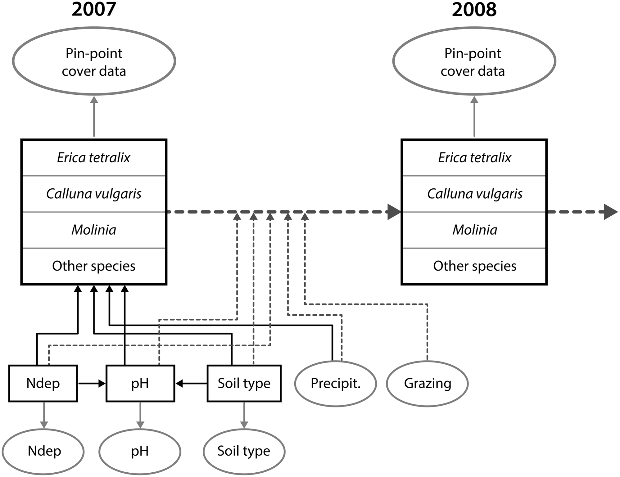
The selected environmental variables were used as the explaining factors to model the observed change in plant cover in a hierarchical SEM, where only linear relationships among the variables were assumed (Damgaard Reference Damgaard2019b). The SEM was based on the current knowledge of the causal relationships among variables and their effects on the vegetation in wet heathlands (Strandberg et al. Reference Strandberg, Damgaard, Degn, Bak and Nielsen2012, Damgaard et al. Reference Damgaard, Thomsen, Borchsenius, Nielsen and Strandberg2013, Reference Damgaard, Strandberg, Kristiansen, Nielsen and Bak2014, Reference Damgaard, Nielsen and Strandberg2017, Lykke et al. Reference Lykke, Strandberg, Nielsen, Barfod and Damgaard2015). Additionally, geographical regional latent effects were modelled after the Danish wet heathland sites were divided into seven geographical regions. The SEM was fitted within a Bayesian hierarchical framework with structural equations and measurement equations in an acyclic directed graph (Fig. 1), where spatial and temporal processes are separated and each arrow is modelled by a conditional likelihood function (Damgaard Reference Damgaard2019b).
Outline of the structural equation model. The spatial variation in vegetation cover in 2007 is modelled by nitrogen deposition (Ndep), soil pH (pH), soil type and precipitation (Precipit.). The yearly change in vegetation cover from 2007 to 2014 (only a single yearly change is shown in the figure) is modelled by all of the former variables as well as grazing. The square boxes are latent variables and the oval boxes are data. The full arrows denote spatial processes and the dotted arrows denote temporal processes (Damgaard Reference Damgaard2019b).

The resulting joint posterior probability distribution of model parameters allowed for the testing of various general ecological hypotheses on how wet heathland vegetation is regulated as well as quantifying the effects of the selected environmental variables on the observed changes in the vegetation. Overall, the temporal model explained the observed changes in plant cover data rather well, and better than the spatial model explained the spatial variation in plant cover data (Damgaard Reference Damgaard2019b). The fitted model showed that the cover of the two dwarf shrubs, bell heather and heather (C. vulgaris), increased with relatively high nitrogen deposition, high pH, sandy soil, low rainfall and absence of grazing. Nitrogen deposition had a non-significant effect on soil pH, but sandy soils had a lower pH. This means that there was both a direct effect of a relatively sandy soil on the vegetation and an indirect effect mediated via a lower pH (Damgaard Reference Damgaard2019b).
The fitted model is a statistical model that summarizes trends and variation in the collected monitoring data, and the observed correlations are not necessarily supported by current ecological working hypotheses. For example, it was surprising that nitrogen deposition on average had a positive effect on the coverage of dwarf shrubs, and this may be explained by possible covariation with other important but unmeasured factors (Damgaard Reference Damgaard2019b).
Local ecological predictions and adaptive management plans
Using the monitoring data and the causal relationships hypothesized in the SEM, it is now possible to generate ecological predictions at a local site where an adaptive management plan is required. The globally fitted information on the causal relationships at all of the monitored sites is contained in the joint posterior probability distribution of the model parameters. Therefore, the probability distribution of the modelled ecological variable at the local site at some time in the future may be calculated from the joint posterior probability distribution by inserting local values of the ecological and environmental variables into the temporal SEM.
The probability distribution of the predicted cover of bell heather after 5 years at a hypothetical wet heathland site, where we want to make ecological predictions, was calculated under different scenarios, assuming that the initial cover of bell heather was 5%. Here, four scenarios were investigated: with and without grazing by livestock at two different soil pH values. The values of the other ecological and selected environmental variables were set within a realistic range for Danish conditions: nitrogen deposition, soil and precipitation were assumed to be 15 kg N ha–1 year–1, coarse sandy soil and 700 mm year–1, respectively. The initial covers of C. vulgaris, M. caerulea and the aggregated class of all other higher plant species were set to 30%, 30% and 35%, respectively. The geographical region of the site was not specified (i.e., there were no geographical regional latent effects).
In order to insert local values of the ecological and environmental variables into the temporal SEM, some of these variables have to be measured at the local site. If the local ecological and environmental measurements are based on a sample of c. 40 plots, this should be sufficient to obtain the required precision for making credible ecological predictions. Compared to the cost of the different management practices, it is relatively inexpensive to collect the necessary environmental and ecological data, and, in addition, the collected data can be used to document the effect of the management. In the following ecological predictions, it is assumed that the values of the environmental variables are known with high precision. However, any sampling and measurement errors of the ecological and environmental variables may be incorporated into the ecological predictions using standard methods (Carroll et al. Reference Carroll, Ruppert, Stefanski and Crainiceanu2006).
All calculations are made using Mathematica (Wolfram Reference Wolfram2020), and the Mathematica notebook is provided in Electronic Supplement S1.
Generic framework
Generally, the above-described procedure may be described by the following generic expressions. The joint posterior probability distribution of model parameters,
 $$\theta $$
, after applying a relevant model to environmental and ecological monitoring data,
 $$Y$$
, is denoted
 $$p\left( {\theta ,Y} \right)$$
.
Generally, the above-described procedure may be described by the following generic expressions. Assume the independent environmental variables (e.g., soil texture, pH, climate) are denoted X and the dependent ecological variables (e.g., plant and animal population sizes), which are needed for making the adaptive management plan, are denoted Y. Furthermore, the values of the independent environmental variables at the local site where an adaptive management plan is required are denoted X′, the initial values of the dependent ecological variables at the local site are measured and denoted
 $$Y_0^\prime $$
and the values of the dependent variable at the local site at a certain time in the future are denoted
 $$Y_t^\prime $$
. Then the predicted posterior probability distribution of
$$Y_t^\prime $$
, which is required for making the adaptive management plan, may be calculated as
 $$p(Y_t^\prime |Y_0^\prime ,X^\prime ) = \smallint p(Y_t^\prime |Y_0^\prime ,X^\prime ,\theta )p(\theta |Y,X)d\theta $$
where
 $$p(\theta |Y,X)$$
is the posterior probability distribution of the model parameters obtained from all of the sites.
In the presented case study, a hierarchical SEM (see Electronic Supplement S2) was used to model the spatial and temporal effects, and this model type has several advantages when making ecological predictions: (1) it is possible to account for measurement and sampling error among both the environmental and ecological variables; (2) it is possible to partition the variance into its different components – there only some of the components (e.g., process error) that may be relevant for the ecological predictions; and (3) it is possible to account for unmeasured variables or instrument variables in the SEM framework. It has been demonstrated that failure to account for the abovementioned effects may lead to sizable prediction bias (Damgaard Reference Damgaard2020, Rinella et al. Reference Rinella, Strong and Vermeire2020, Damgaard & Weiner Reference Damgaard and Weiner2021).
Results
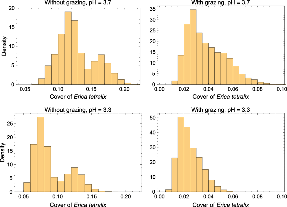
If the initial cover of bell heather was 5% at a wet heathland site and the conservation goal was set to 10% cover of bell heather after 5 years, then the probability of achieving this goal depends on both soil pH at the site and whether grazing is part of the management practice (Fig. 2). If the soil pH at the site is relatively high, the probability of reaching the conservation goal increases, whereas grazing by livestock is predicted to have an important negative effect on the probability of achieving the conservation goal (Fig. 2). Unfortunately, the grazing data only consist of a binary recording of whether there were signs of grazing by livestock, and there are no data on which livestock were used to graze the site, their stocking density or when the sites had been grazed. Therefore, the estimated effect of grazing on the vegetation at wet heathland sites is only credible when grazing by livestock is performed in a way that is typical for the sites where the monitoring data have been collected. In Denmark, grazing by livestock in wet heathland sites mainly occurs in the plant growth period from May to October. The most commonly used species of livestock are sheep, although cows or ponies may also be used. The recommended stocking density of large herbivores for Danish wet heathlands is less than 0.5 herbivore equivalents per hectare, where an adult sheep counts as 0.15 of a large herbivore (Miljøstyrelsen n.d.). Consequently, the model predicted effect of grazing is expected to be credible for summer grazing by sheep at the recommended stocking rate, whereas the predicted effect of whole-year grazing by ponies is less credible, for example.
Probability densities of the predicted cover of bell heather (Erica tetralix) after 5 years with an initial cover of 5%. Four scenarios were examined: with and without grazing at two levels of soil pH. The local nitrogen deposition, soil and precipitation are assumed to be 15 kg N ha–1 year–1, coarse sandy soil and 700 mm year–1, respectively.

In this demonstration of the method, only soil pH and grazing varied, but if any of the other environmental variables at the hypothetical local site had varied, this would also affect the probability of achieving the conservation goal (results not shown).
Since the probability of reaching the conservation goal is calculated as probability densities, the uncertainty of reaching the goal is automatically calculated and shown in a transparent way. The source of this uncertainty is mainly variation in the temporal processes among the monitored 39 wet heathland sites, and it is expected that this number of sites is sufficiently high to contain most of the variation in the studied temporal processes at Danish wet heathland sites.
The actual adaptive management plan will depend on local conditions, stakeholders and previous experience of different management actions on wet heathlands (Williams et al. Reference Williams, Szaro and Shapiro2009). However, according to the fitted temporal SEM, it is highly unlikely that the conservation goal of 10% cover of bell heather would be reached if the local site is grazed, so it would not be realistic or credible to suggest grazing by livestock as the only management practice in the adaptive management plan. Furthermore, if the cover of bell heather in the absence of grazing decreases to a threshold level specified in the adaptive management plan (e.g., 3%), then it may be concluded that the local dynamics are atypical and the adaptive management plan must contain alternative management actions for this case (e.g., cutting and burning) (Hampton Reference Hampton2008). In all cases, it will be important to document the effect of the management for future learning and more specific ecological modelling of the effect of different management practices on wet heathlands.
Discussion
In this demonstration study, I have focused on predicting the effect of grazing on wet heathlands that differ in soil pH. Such ecological predictions of relevant ecological variables may be used to generate adaptive management plans. For example, suppose that the conservation goal in a nature conservation project of a wet heathland site is to increase the cover of bell heather from 5% to 10% over a 5-year period. Then it will be relevant to calculate the probability distribution of observing such an increase in the cover of bell heather under different management scenarios. The calculated probability distributions of the expected change in the cover of bell heather will: (1) help the local manager to select among different management strategies, such that the management at the site is in agreement with the conservation goals; and (2) help to set threshold levels in the adaptive management plan where the local management strategy should be reconsidered. For example, if the cover of bell heather drops significantly below the initial 5% and model predictions have shown such a change in cover to be unlikely, then the dynamics at the local site are not in agreement with the majority of the monitored wet heathland sites and the manager must consider alternative management strategies.
As demonstrated here and in Damgaard (Reference Damgaard2019b), grazing by livestock is expected to reduce the cover of cross-leaved heath. Consequently, based on these results, grazing by livestock on wet heathlands with a relatively low cover of cross-leaved heath cannot be recommended as the only management practice. The effect of grazing has previously been investigated in adaptive management schemes. For example, Davis et al. (Reference Davis, Augustine, Monroe, Derner and Aldridge2020) predicted the effect of different grazing regimes on bird population sizes.
The presented approach is generic, and different types of ecological monitoring data may be used to generate local ecological predictions and adaptive management plans. More specifically, SEMs are currently being fitted to monitoring data of other light, open habitat types (e.g., acid grasslands and dry heathlands).
It is now timely to revisit the practice of how the uncertainties of adaptive management plans are quantified. In many applied cases of ecological and environmental modelling there is sizeable variation in the measured independent variables due to measurement and sampling error (Muff et al. Reference Muff, Riebler, Held, Rue and Saner2015, Yanai et al. Reference Yanai, See and Campbell2018). For example, the soil type in the presented case study was determined with relatively large uncertainty (Damgaard Reference Damgaard2019b), and such measurement uncertainties have been shown to lead to regression dilution and sizable prediction bias (Damgaard Reference Damgaard2020, Damgaard & Weiner Reference Damgaard and Weiner2021). Furthermore, the importance of accounting for unmeasured variables or instrument variables in SEMs used for predictive purposes has also been demonstrated (Rinella et al. Reference Rinella, Strong and Vermeire2020, Grace Reference Grace2021). Since the uncertainties of the ecological predictions are quantified by probability distributions, the ecological predictions will also suggest levels of the ecological variables that may act as early warning signs in the adaptive management plans for changing the management at the site. For example, if the cover of bell heather in an ungrazed wet heathland site decreases from an initial level of 5%, then the development at the site may be reasoned to be atypical and alternative measures need to be considered.
For some management practices, there may be important time lags between the onset of the management practice and when the effect of the management may be observed in the ecosystem. Such time lags are usually not incorporated in standard ecological predictive models and must be considered and incorporated into the adaptive management plans.
Some environmental data that are important for the regulation of the studied ecosystem may not be available (e.g., distance to water table data or better grazing data). Such unmeasured or poorly measured variables will surely increase the uncertainties of the ecological predictions compared to a situation where the data are available and the variable is included in the SEM. However, if the unmeasured variables at the local site are within the domain of the unmeasured variables of the sites that are monitored (i.e., the local site is not atypical), then the local ecological predictions most likely will be unbiased. We may criticize statistical models for a lack of precision and for not including all relevant information; however, we will not get sufficient data to make absolute precise local ecological predictions in our lifetime – perhaps never. If we cannot obtain absolute precision, then the next best option is to quantify our uncertainty. Quantitative adaptive management plans, which may be assessed and evaluated by the competent authorities, may also lead to higher societal investments in biodiversity management, since the possible benefits and risks of the investment have been quantified.
In Denmark, ecological monitoring data are collected as part of the national responsibility outlined in the EU Habitats Directive (EU 1992) and are primarily used to report on the conservation status of the different terrestrial habitats. Why not put the often-excellent ecological monitoring data that are already being collected in many countries to practical use by generating quantitative and credible local adaptive management plans? Next, is the current generation of applied ecologists and local managers of natural habitats ready to embrace the quantitative methods of ecological predictions?
Acknowledgements
None.
Financial support
None.
Conflict of interest
None.
Ethical standards
None.