1. Introduction
Rotating shear flows are common in nature. Geophysical and astrophysical examples include the interiors of planets and stars, planetary atmospheres, and stellar and planetary accretion disks. Since direct observations and measurements are hard to perform for many of these flows, laboratory models that incorporate the essential features of these flows can be useful. A common simple rotating shear flow that can be implemented in the laboratory is Taylor–Couette (TC) flow, which is the flow in the fluid-filled gap between two coaxial rotating cylinders. Taylor–Couette flow has found particular applicability as a model for astrophysical accretion disks in determining their stability properties and the outward angular momentum flux that is necessary in order for material to be transported inwards towards the central body (Zeldovich Reference Zeldovich1981; Richard & Zahn Reference Richard and Zahn1999; Richard Reference Richard2001; Dubrulle et al. Reference Dubrulle, Dauchot, Daviaud, Longaretti, Richard and Zahn2005a ; Ji & Balbus Reference Ji and Balbus2013). Taylor–Couette experiments have produced contradictory answers to these questions, causing great debate centred on the effects of the no-slip axial boundaries found in Taylor–Couette experiments which do not match the open stratified boundaries of accretion disks (Balbus Reference Balbus2011; Avila Reference Avila2012; Schartman et al. Reference Schartman, Ji, Burin and Goodman2012; Ji & Balbus Reference Ji and Balbus2013; Edlund & Ji Reference Edlund and Ji2014).
We can define a Reynolds number for the inner (outer) cylinder using the radius
 $r_{i}(r_{o})$
, the rotation rate
 ${\it\Omega}_{i}({\it\Omega}_{o})$
and the fluid kinematic viscosity
 ${\it\nu}$
, giving
 $$\begin{eqnarray}\mathit{Re}_{i}=\frac{{\it\Omega}_{i}\,r_{i}(r_{o}-r_{i})}{{\it\nu}},\quad \mathit{Re}_{o}=\frac{{\it\Omega}_{o}\,r_{o}(r_{o}-r_{i})}{{\it\nu}}.\end{eqnarray}$$
Rather than using
 $\mathit{Re}_{i}$
and
 $\mathit{Re}_{o}$
, we use the shear Reynolds number
 $\mathit{Re}_{S}$
and the so-called
 $q$
parameter, detailed below, to compare different parts of the parameter space. They have a more intuitive relation to the shear and the global rotation. The shear Reynolds number
 $\mathit{Re}_{S}\propto |{\it\Omega}_{i}-{\it\Omega}_{o}|$
, which quantifies shear, is defined as
 $$\begin{eqnarray}\mathit{Re}_{S}=\frac{2}{1+{\it\eta}}|\mathit{Re}_{i}-{\it\eta}\mathit{Re}_{o}|,\end{eqnarray}$$
where
 ${\it\eta}=r_{i}/r_{o}$
is the radius ratio (Dubrulle et al.
Reference Dubrulle, Dauchot, Daviaud, Longaretti, Richard and Zahn2005a
). Next to
 ${\it\eta}$
, another important geometric quantity is the aspect ratio
 ${\it\Gamma}=L/(r_{o}-r_{i})$
, which is the ratio of the height of the cylinders
 $L$
to the gap width. To quantify the global rotation, we use the
 $q$
parameter (Ji et al.
Reference Ji, Burin, Schartman and Goodman2006; Schartman et al.
Reference Schartman, Ji, Burin and Goodman2012) defined through the relation
 $$\begin{eqnarray}\frac{{\it\Omega}_{i}}{{\it\Omega}_{o}}={\it\eta}^{-q}.\end{eqnarray}$$
The
 $q$
parameter is real for co-rotating cylinders, the case exclusively dealt with in this paper. Hence, we will define both
 ${\it\Omega}_{i}$
and
 ${\it\Omega}_{o}$
to be positive throughout this paper. Solid-body rotation
 ${\it\Omega}_{i}={\it\Omega}_{o}$
corresponds to
 $q=0$
,
 ${\it\Omega}_{i}>{\it\Omega}_{o}$
gives
 $q>0$
,
 ${\it\Omega}_{i}<{\it\Omega}_{o}$
gives
 $q<0$
, and pure inner and pure outer rotation correspond to
 $q=+\infty$
and
 $q=-\infty$
respectively.
Different dimensionless parameters other than
 $\mathit{Re}_{S}$
and
 $q$
have been used, which are presented here for ease of comparison. Rather than using
 $\mathit{Re}_{S}$
to quantify the shear, previous work on our apparatus (van Gils et al.
Reference van Gils, Huisman, Bruggert, Sun and Lohse2011b
, Reference van Gils, Huisman, Grossmann, Sun and Lohse2012) has used a Taylor number
 $\mathit{Ta}=({\it\sigma}\,\mathit{Re}_{S})^{2}$
, where
 ${\it\sigma}=(1+{\it\eta})^{4}/(2\sqrt{{\it\eta}})^{4}$
is a geometric Prandtl number (Eckhardt, Grossmann & Lohse Reference Eckhardt, Grossmann and Lohse2007), which equals 1.057 for our
 ${\it\eta}=0.716$
. With a nearly identical geometry, Paoletti & Lathrop (Reference Paoletti and Lathrop2011) used a different definition of the Reynolds number, namely
 $\mathit{Re}=\sqrt{{\it\sigma}}\,\mathit{Re}_{S}=\sqrt{\mathit{Ta }/{\it\sigma}}$
. Another parameter quantifying global rotation is the rotation parameter,
 $R_{{\it\Omega}}$
(Dubrulle et al.
Reference Dubrulle, Dauchot, Daviaud, Longaretti, Richard and Zahn2005a
), defined as
 $R_{{\it\Omega}}=(1-{\it\eta})(\mathit{Re}_{i}+\mathit{Re}_{o})/({\it\eta}\mathit{Re}_{o}-\mathit{Re}_{i})$
.
At low
 $\mathit{Re}_{S}$
, before the formation of Taylor vortices, and in the absence of Ekman pumping from axial boundaries (e.g. periodic or free-slip axial boundary conditions), the azimuthal velocity profile is
 $$\begin{eqnarray}u_{{\it\theta},lam}(r)=Ar+\frac{B}{r},\quad A=\frac{{\it\Omega}_{o}-{\it\eta}^{2}{\it\Omega}_{i}}{1-{\it\eta}^{2}},~B=\frac{r_{i}^{2}({\it\Omega}_{i}-{\it\Omega}_{o})}{1-{\it\eta}^{2}}.\end{eqnarray}$$
We will refer to this as laminar Taylor–Couette flow.
Some rotating flows have radially increasing specific angular momentum (
 $\text{sign}(\partial \ell /\partial r)=\text{sign}\,\ell$
), where
 $\ell =r^{2}{\it\omega}$
is the specific angular momentum and
 ${\it\omega}=u_{{\it\theta}}/r$
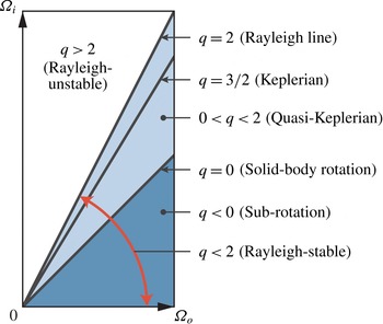
is the fluid angular velocity. Such flows (see figure 1), as long as they are purely hydrodynamic, barotropic and stably stratified as we consider here, are stable to infinitesimal perturbations (i.e. linearly stable) according to the Rayleigh criterion (Rayleigh Reference Rayleigh1917). For Taylor–Couette flow, this corresponds to
 $q<2$
. Flows for which
 $q>2$
are linearly unstable at sufficiently high Reynolds numbers (Taylor Reference Taylor1923); this is often called the centrifugal instability. Hence,
 $q=2$
is referred to as the Rayleigh line. The Rayleigh-stable region includes sub-rotation (
 ${\it\Omega}_{i}<{\it\Omega}_{o}$
), solid-body rotation (
 ${\it\Omega}_{i}={\it\Omega}_{o}$
), and super-rotation (
 ${\it\Omega}_{i}>{\it\Omega}_{o}$
). The flow in the super-rotating region is often referred to as quasi-Keplerian, since it includes cylinder rotation rates (
 $q=3/2$
) obeying Kepler’s third law relating orbital radius and period. This regime is of particular relevance to astrophysical systems such as accretion disks since they are Rayleigh-stable with azimuthal flow profiles in the plane of the disk that are expected to not deviate significantly from Kepler’s third law when ignoring the disk’s self-gravitation and relativistic effects (Richard & Zahn Reference Richard and Zahn1999; Richard Reference Richard2001; Dubrulle et al.
Reference Dubrulle, Dauchot, Daviaud, Longaretti, Richard and Zahn2005a
; Ji & Balbus Reference Ji and Balbus2013).
The Taylor–Couette parameter space considered here (red arrow). The different regions are shown as well as three important lines of constant
 $q$
: the Rayleigh line (
 $q=2$
), the Keplerian line (
 $q=3/2$
) and solid-body rotation (
 $q=0$
). The whole Rayleigh-stable region (
 $q<2$
) is shaded with different colours for the quasi-Keplerian regime (light blue) and the sub-rotating regime (dark blue).

Accretion disks are Rayleigh-stable but are known to have accretion rates requiring radial fluxes of angular momentum far greater than the flux provided by viscous diffusion in laminar Taylor–Couette flow-like disks, indicating that they are in fact unstable (Richard & Zahn Reference Richard and Zahn1999; Richard Reference Richard2001; Dubrulle et al. Reference Dubrulle, Dauchot, Daviaud, Longaretti, Richard and Zahn2005a ; Ji & Balbus Reference Ji and Balbus2013). There has been a search for the instabilities at play in these flows. Disks that are sufficiently ionized to be electrically conductive are known to be unstable via the magneto-rotational instability (MRI) (Ji & Balbus Reference Ji and Balbus2013, and description therein). For weakly ionized disks or parts of disks, investigation has focused on stability in the presence of stratification (Dubrulle et al. Reference Dubrulle, Marié, Normand, Richard, Hersant and Zahn2005b ; Le Bars & Le Gal Reference Le Bars and Le Gal2007; Le Dizès & Riedinger Reference Le Dizès and Riedinger2010) and stability to finite amplitude perturbations (nonlinear stability) which has been the subject of several Taylor–Couette experiments including our own in this paper (Richard Reference Richard2001; Ji et al. Reference Ji, Burin, Schartman and Goodman2006; Paoletti & Lathrop Reference Paoletti and Lathrop2011; Paoletti et al. Reference Paoletti, van Gils, Dubrulle, Sun, Lohse and Lathrop2012; Schartman et al. Reference Schartman, Ji, Burin and Goodman2012; Edlund & Ji Reference Edlund and Ji2014).
For an incompressible fluid in the Rayleigh-stable region of Taylor–Couette flow and compressible accretion disk flow, the possibility of a nonlinear instability has not yet been ruled out for all
 $\mathit{Re}_{S}$
. Plane Couette flow and pipe flow are both examples of linearly stable flows that have nonlinear instabilities at sufficient
 $\mathit{Re}$
(Grossmann Reference Grossmann2000; Avila et al.
Reference Avila, Moxey, de Lozar, Avila, Barkley and Hof2011; Shi, Avila & Hof Reference Shi, Avila and Hof2013, and references therein). Maretzke, Hof & Avila (Reference Maretzke, Hof and Avila2014) found transient growth, a necessary prerequisite for a nonlinear instability, in Rayleigh-stable Taylor–Couette flow. Accretion disks have very high Reynolds numbers, with
 $\mathit{Re}_{S}$
possibly as high as
 $10^{14}$
(Paoletti et al.
Reference Paoletti, van Gils, Dubrulle, Sun, Lohse and Lathrop2012; Ji & Balbus Reference Ji and Balbus2013). Therefore, it is reasonable to ask whether Rayleigh-stable Taylor–Couette flow is nonlinearly stable or unstable.
In prior experimental work, visualization via Kalliroscope particles, angular momentum transport measurements and velocimetry measurements have been performed, yielding contradictory results on the presence of a nonlinear instability, especially for quasi-Keplerian flow (Wendt Reference Wendt1933; Taylor Reference Taylor1936a ,Reference Taylor b ; Coles Reference Coles1965; Richard Reference Richard2001; Ji et al. Reference Ji, Burin, Schartman and Goodman2006; Borrero-Echeverry, Schatz & Tagg Reference Borrero-Echeverry, Schatz and Tagg2010; Paoletti & Lathrop Reference Paoletti and Lathrop2011; Burin & Czarnocki Reference Burin and Czarnocki2012; Paoletti et al. Reference Paoletti, van Gils, Dubrulle, Sun, Lohse and Lathrop2012; Schartman et al. Reference Schartman, Ji, Burin and Goodman2012; Edlund & Ji Reference Edlund and Ji2014). These experiments have, to varying degree, Ekman pumping driven by the no-slip boundary conditions on the axial boundaries. The Ekman pumping could destabilize the flow depending on the axial end configuration in a way that would not be found in astrophysical accretion disks (Balbus Reference Balbus2011; Avila Reference Avila2012; Schartman et al. Reference Schartman, Ji, Burin and Goodman2012; Ji & Balbus Reference Ji and Balbus2013; Edlund & Ji Reference Edlund and Ji2014), which have open stratified axial boundaries. Axial boundaries that rotate with the outer cylinder, such as those on the apparatus presented in this paper, were found to have Ekman pumping effects that spanned the whole flow volume (Avila Reference Avila2012; Schartman et al. Reference Schartman, Ji, Burin and Goodman2012; Edlund & Ji Reference Edlund and Ji2014), which might explain the large, and probably turbulent, angular momentum transport found by the Maryland experiment (Paoletti & Lathrop Reference Paoletti and Lathrop2011), in contrast to the low-angular-momentum-transport steady laminar flow found in the Princeton MRI and HTX experiments which reduced the Ekman pumping by splitting the axial boundaries into rings rotated at speeds intermediate to those of the two cylinders (Ji et al. Reference Ji, Burin, Schartman and Goodman2006; Schartman et al. Reference Schartman, Ji, Burin and Goodman2012; Edlund & Ji Reference Edlund and Ji2014).
The effect of the Ekman pumping in wide-gap (
 ${\it\eta}<0.34$
) low-aspect-ratio (
 ${\it\Gamma}<3$
) Rayleigh-stable experiments, such as the Princeton MRI and HTX experiments, on the flow state and angular momentum transport has been the subject of several investigations. When the axial boundaries are attached to the outer cylinder as opposed to rotating at intermediate speeds, there are large fluctuations and mixing near the inner cylinder (Dunst Reference Dunst1972; Edlund & Ji Reference Edlund and Ji2014), and quiescent flow rotating close to
 ${\it\Omega}_{o}$
near the outer cylinder (Dunst Reference Dunst1972; Kageyama et al.
Reference Kageyama, Ji, Goodman, Chen and Shoshan2004; Schartman et al.
Reference Schartman, Ji, Burin and Goodman2012; Edlund & Ji Reference Edlund and Ji2014). Speeding up the part of the axial boundaries near the inner cylinder causes the fluctuations near the inner cylinder to decrease and the azimuthal velocities to more closely match laminar Taylor–Couette flow (Edlund & Ji Reference Edlund and Ji2014). In the reduced Ekman pumping configuration, perturbations by jets from the inner cylinder were found to decay for
 $\mathit{Re}_{S}\leqslant 10^{6}$
(Edlund & Ji Reference Edlund and Ji2014).
The effect of the Ekman pumping in medium-gap (
 ${\it\eta}\approx 0.7$
) larger-aspect-ratio (
 ${\it\Gamma}\sim 10$
) experiments, such as the Maryland and our experiments, has not received as much attention, although it is expected to be similar, which would resolve the contradictory results. At low
 $\mathit{Re}_{S}<10^{4}$
, axial boundaries attached to the outer cylinder were found to destabilize the flow (Avila Reference Avila2012). For
 $\mathit{Re}_{S}\leqslant 10^{5}$
direct numerical simulations (DNS) with periodic axial boundaries in the quasi-Keplerian regime, Ostilla-Mónico et al. (Reference Ostilla-Mónico, Verzicco, Grossmann and Lohse2014) found that initially turbulent states always decayed to laminar Taylor–Couette flow. In this paper, we present azimuthal velocimetry profiles in both the quasi-Keplerian and the sub-rotating regimes in a geometry similar to the Maryland experiment. We compare them with the profiles in laminar Taylor–Couette flow and discuss their structure to better elucidate the effects of Ekman pumping on the flow and the large angular momentum transport associated with axial boundaries fixed to the outer cylinder for our geometry (Paoletti & Lathrop Reference Paoletti and Lathrop2011).
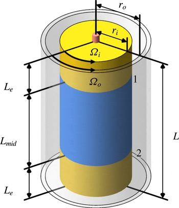
Sketch of the
 $\text{T}^{3}\text{C}$
apparatus used for the measurements presented in this paper. The inner cylinder is split into three sections, having a 2.5 mm gap between each section, marked as positions 1 and 2.

The paper is organized as follows: § 2 describes the experiment and the parameter space explored, § 3 presents the azimuthal velocity and specific angular momentum profiles, § 4 presents further analysis and discussion of the azimuthal profiles including the primarily axial transport of angular momentum, and § 5 summarizes the results and presents conclusions.
2. The experiment and the parameter space explored
The apparatus is described in detail in van Gils et al. (Reference van Gils, Bruggert, Lathrop, Sun and Lohse2011a
) and is shown schematically in figure 2. A brief summary is given here. The inner cylinder has an outer radius of
 $r_{i}=20.00~\text{cm}$
and the transparent outer cylinder has an inner radius of
 $r_{o}=27.94~\text{cm}$
, which gives
 ${\it\eta}=0.716$
. They can rotate independently up to maxima of
 $|{\it\Omega}_{i}/2{\rm\pi}|=20~\text{Hz}$
and
 $|{\it\Omega}_{o}/2{\rm\pi}|=10~\text{Hz}$
respectively. The total height is
 $L=93.2~\text{cm}$
, which gives
 ${\it\Gamma}=11.74$
. The axial boundaries are attached to the outer cylinder. The inner cylinder is split into three sections. The height of the middle section is
 $L_{mid}=53.6~\text{cm}$
, and the end sections have equal heights of
 $L_{e}=19.35~\text{cm}$
. There is a 2.5 mm gap between each section, labelled 1 and 2 in figure 2. The system was filled with water and operated at room temperature with cooling applied at the axial boundaries. This geometry is similar to the apparatus used by Paoletti & Lathrop (Reference Paoletti and Lathrop2011), who have an
 ${\it\eta}=0.7245$
and
 ${\it\Gamma}=11.47$
geometry.
The azimuthal velocity profiles were obtained using laser Doppler anemometry (LDA). The LDA configuration used backscatter from seed particles in a measurement volume of approximately
 $0.07~\text{mm}\times 0.07~\text{mm}\times 0.3~\text{mm}$
. Dantec PSP-5 particles with a
 $5~{\rm\mu}\text{m}$
diameter and
 $1.03~\text{g}~\text{cm}^{-3}$
density were used. The optical effect of the outer cylinder curvature on the LDA measurements was corrected by using the calculations of Huisman, van Gils & Sun (Reference Huisman, van Gils and Sun2012b
). The velocimetry was calibrated using radial and axial profiles of solid-body rotation at different rotation rates. The error in the mean velocity profiles from the calibration, which was the dominant source in the mean profiles, was smaller than 0.1 %. For all LDA measurements a statistical convergence of 1 % was achieved, which translates to between 1 % and 6 % of
 $|{\it\Omega}_{i}-{\it\Omega}_{o}|$
, which prevents investigation into fluctuations and deviations from axisymmetry. When measuring close to the inner cylinder, reflections from the metal inner cylinder were found to be problematic. Hence, the radial profiles presented in this paper were performed at the axial height of the 2.5 mm gap between the bottom and middle inner cylinder sections, which corresponds to an axial height
 $z/L=0.209$
off the bottom, so that the LDA laser would be absorbed in the gap as opposed to being reflected off the cylinder surface. The axial dependence of the angular velocity was found to be less than 2 % of
 $|{\it\Omega}_{i}-{\it\Omega}_{o}|$
from axial profiles at midgap from midheight to 1.5 cm off the bottom, and between radial profiles over the outer half of the gap at five heights
 $z=\{0.195,0.223,0.414,0.464,0.927\}~\text{m}$
off the bottom, which are at
 $z/L=\{0.209,0.238,0.444,0.497,0.995\}$
. The last one,
 $z/L=0.995$
, is 5 mm from the top axial boundary. Thus, a radial profile at
 $z/L=0.209$
is representative, other than possibly for radial positions closer than 2.5 mm to the inner cylinder. The boundary layers on the axial boundaries are confined to within 5 mm of the boundaries.
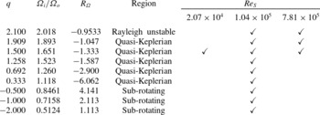
Velocimetry was performed for five quasi-Keplerian
 $q$
values including Keplerian (
 $q=1.500$
), three sub-rotating values of
 $q$
, and one unstable but very close to the Rayleigh line
 $q$
value (
 $q=2.100$
), which are all listed in table 1. The value
 $q=1.909$
was chosen to match the simulations of Avila (Reference Avila2012) on a nearly identical geometry and the Princeton experimental work at
 $q=1.9$
(Ji et al.
Reference Ji, Burin, Schartman and Goodman2006; Schartman et al.
Reference Schartman, Ji, Burin and Goodman2012). Additionally,
 $q=\{1.909,1.500,1.258,0.692\}$
were chosen to match ongoing torque measurements on the Maryland experiment. Measurements for all values of
 $q$
were taken at
 $\mathit{Re}_{S}=1.04\times 10^{5}$
, the three values of
 $q\geqslant 1.500$
at
 $\mathit{Re}_{S}=7.81\times 10^{5}$
, and
 $q=1.500$
at
 $\mathit{Re}_{S}=2.07\times 10^{4}$
. All of the azimuthal velocity profiles, the radial profiles at all five heights and the axial profile at midgap are available in the supplementary data available at http://dx.doi.org/10.1017/jfm.2015.275. Each pair of
 $q$
and
 $\mathit{Re}_{S}$
was reached by starting with both cylinders at rest, linearly increasing
 ${\it\Omega}_{i}$
and
 ${\it\Omega}_{o}$
to their final values over 120 s while maintaining constant
 $q$
, and then waiting at least 600 s for transients to decay before performing measurements.
The
 $q$
values for which velocity profiles were measured and their corresponding rotation rate ratios (
 ${\it\Omega}_{i}/{\it\Omega}_{o}$
) and rotation parameter,
 $R_{{\it\Omega}}$
. We also give the region of the Taylor–Couette parameter space the measurement is in, and for what
 $\mathit{Re}_{S}$
measurements were taken.

3. Results on the azimuthal profiles
It is convenient to look at the velocity profiles in terms of the normalized radial position and the normalized angular velocity given by
 $$\begin{eqnarray}\displaystyle & \displaystyle \widetilde{r}=\frac{r-r_{i}}{d}, & \displaystyle\end{eqnarray}$$
 $$\begin{eqnarray}\displaystyle & \displaystyle \widetilde{{\it\omega}}=\frac{{\it\omega}-{\it\Omega}_{o}}{{\it\Omega}_{i}-{\it\Omega}_{o}}, & \displaystyle\end{eqnarray}$$
 $d=r_{o}-r_{i}$
is the width of the gap. The expression for
 $\widetilde{r}$
gives
 $\widetilde{r}=0$
at the inner cylinder and
 $\widetilde{r}=1$
at the outer cylinder. Regardless of which cylinder has the larger angular velocity, the expression for
 $\widetilde{{\it\omega}}$
gives
 $\widetilde{{\it\omega}}=0$
whenever
 ${\it\omega}={\it\Omega}_{o}$
and
 $\widetilde{{\it\omega}}=1$
whenever
 ${\it\omega}={\it\Omega}_{i}$
. For the quasi-Keplerian regime,
 $\widetilde{{\it\omega}}>1$
indicates a super-rotating flow with
 ${\it\omega}>{\it\Omega}_{i}>{\it\Omega}_{o}>0$
and
 $\widetilde{{\it\omega}}<0$
indicates a sub-rotating flow with
 ${\it\Omega}_{i}>{\it\Omega}_{o}>{\it\omega}$
. Due to the sign change in the denominator for the sub-rotating regime,
 $\widetilde{{\it\omega}}>1$
indicates a sub-rotating flow with
 ${\it\Omega}_{o}>{\it\Omega}_{i}>{\it\omega}$
and
 $\widetilde{{\it\omega}}<0$
implies a super-rotating flow with
 ${\it\omega}>{\it\Omega}_{o}>{\it\Omega}_{i}>0$
. The laminar Taylor–Couette profile, which in these normalized variables is independent of
 ${\it\Omega}_{i}$
and
 ${\it\Omega}_{o}$
, is
 $$\begin{eqnarray}\widetilde{{\it\omega}}_{lam}=\frac{{\it\eta}^{2}(1-\widetilde{r})(\widetilde{r}(1-{\it\eta})+1+{\it\eta})}{(1+{\it\eta})(\widetilde{r}(1-{\it\eta})+{\it\eta})^{2}}.\end{eqnarray}$$
The
 $\widetilde{{\it\omega}}$
profiles for all values of
 $q$
at
 $\mathit{Re}_{S}=1.04\times 10^{5}$
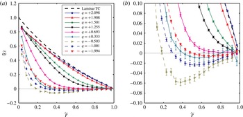
are compared with each other and with the laminar Taylor–Couette profile in figure 3. None of the profiles matched the laminar Taylor–Couette profile. On approaching solid-body rotation (
 $q\rightarrow 0$
) at fixed
 $\mathit{Re}_{S}$
in both regimes, deviation from the laminar Taylor–Couette profile increases and the part of the profile near the inner cylinder steepens. For the quasi-Keplerian regime, as we approach solid-body rotation, the rest of the profile flattens towards
 $\widetilde{{\it\omega}}=0$
. For the sub-rotating regime,
 $\widetilde{{\it\omega}}<0$
away from the inner cylinder. This indicates that the fluid is super-rotating in terms of angular velocity compared with both cylinders (
 ${\it\omega}>{\it\Omega}_{o}>{\it\Omega}_{i}>0$
), with the degree of super-rotation, as a fraction of
 $|{\it\Omega}_{i}-{\it\Omega}_{o}|$
, increasing as we approach solid-body rotation. This flow super-rotation will be further discussed in § 4.1.
Comparison of the normalized angular velocity
 $\widetilde{{\it\omega}}=({\it\omega}-{\it\Omega}_{o})/({\it\Omega}_{i}-{\it\Omega}_{o})$
profiles across the gap for different values of the
 $q$
parameter at
 $\mathit{Re}_{S}=1.04\times 10^{5}$
. (a) The full scale of
 $\widetilde{{\it\omega}}$
(the error bars are smaller than the symbols). (b) An expansion around
 $\widetilde{{\it\omega}}=0$
, using the same symbols to emphasize the parts of the profiles close to rotation at
 ${\it\Omega}_{o}$
. Connecting lines are drawn to guide the eye. The profile for laminar Taylor–Couette flow is drawn for comparison.

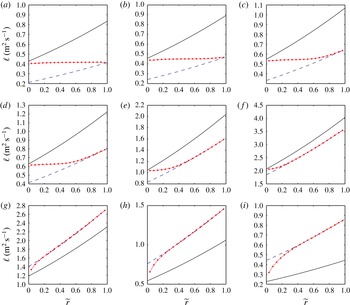
The resulting profiles of the specific angular momentum
 $\ell =r^{2}{\it\omega}$
at
 $\mathit{Re}_{S}=1.04\times 10^{5}$
are shown in figure 4. For the quasi-Keplerian regime, the specific angular momentum profiles all follow the same pattern of having an inner flat region connected to an outer region rotating at
 ${\it\Omega}_{o}$
, which will be discussed further in § 4.2. The flat region in
 $\ell$
indicates that the flow was well mixed in that region.
The specific angular momentum (
 $\ell =r^{2}{\it\omega}$
) profiles across the gap for the different
 $q$
values at
 $\mathit{Re}_{S}\approx 1.04\times 10^{5}$
. The red circles (●) are the specific angular momentum profiles of the flow, with connecting lines to guide the eye. The error bars are smaller than the symbols. The solid black line (——) and dashed blue line (– – –) are the specific angular momentum profiles for
 ${\it\omega}(\widetilde{r})={\it\Omega}_{i}$
and
 ${\it\omega}(\widetilde{r})={\it\Omega}_{o}$
respectively. The vertical axes have the same units and the horizontal axes are the same for all plots. The Keplerian configuration is shown in (c). (a)
 $q=+2.098$
,
 $Re_{S}=1.03\times 10^{5}$
; (b)
 $q=+1.908$
,
 $Re_{S}=1.03\times 10^{5}$
; (c)
 $q=+1.501$
,
 $Re_{S}=1.03\times 10^{5}$
; (d)
 $q=+1.255$
,
 $Re_{S}=1.03\times 10^{5}$
; (e)
 $q=+0.693$
,
 $Re_{S}=1.04\times 10^{5}$
; (f)
 $q=+0.333$
,
 $Re_{S}=1.05\times 10^{5}$
; (g)
 $q=-0.503$
,
 $Re_{S}=1.05\times 10^{5}$
; (h)
 $q=-1.001$
,
 $Re_{S}=1.04\times 10^{5}$
; (i)
 $q=-1.994$
,
 $Re_{S}=1.03\times 10^{5}$
.

Keplerian (
 $q=+1.500$
) profiles for three different
 $\mathit{Re}_{S}$
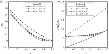
are compared in figure 5. They all have a similar shape, but as
 $\mathit{Re}_{S}$
is increased,
 $\widetilde{{\it\omega}}$
decreases towards solid-body rotation at
 ${\it\Omega}_{o}$
, especially in the outer parts of the gap. In terms of the specific angular momentum, increasing
 $\mathit{Re}_{S}$
leads to a sharper transition between the flat region and the rotation at
 ${\it\Omega}_{o}$
region.
Comparison of the normalized angular velocity and specific angular momentum profiles across the gap for the Keplerian cylinder rotation ratio (
 $q=+1.500$
) at three different
 $\mathit{Re}_{S}$
. (a) The normalized angular velocity
 $\widetilde{{\it\omega}}$
with the laminar Taylor–Couette profile drawn for comparison and (b) the specific angular momentum
 $\ell$
normalized by
 $r_{i}^{2}\,{\it\Omega}_{o}$
with lines for solid-body rotation at the inner and outer cylinder rotation rates (
 $r^{2}{\it\Omega}_{i}$
and
 $r^{2}{\it\Omega}_{o}$
respectively). The error bars are smaller than the symbol heights.

4. Further analysis and discussion
4.1. Super-rotating flow for the sub-rotating regime
As seen in figure 3 for all three sub-rotating profiles,
 $\widetilde{{\it\omega}}<0$
except near the inner cylinder, indicating flow super-rotation (figure 3
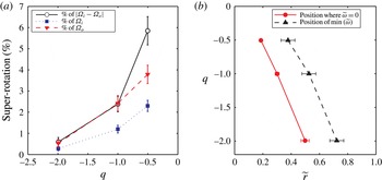
b). The flow super-rotation can be quantified by taking the minimum
 $\widetilde{{\it\omega}}$
in the profile to be the strength of the super-rotation, and finding its radial position along with where the linear interpolation of the profile crosses
 ${\it\omega}={\it\Omega}_{o}(\widetilde{{\it\omega}}=0)$
to super-rotation. The strength of the super-rotation is shown in figure 6(a) and the radial locations of the maximum super-rotation and of
 $\widetilde{{\it\omega}}=0$
are shown in figure 6(b). On approaching solid-body rotation (
 $q\rightarrow 0$
) at fixed non-zero
 $\mathit{Re}_{S}$
, the strength of super-rotation increases, and the radial positions of the super-rotation maximum and
 $\widetilde{{\it\omega}}=0$
both move towards the inner cylinder. This is a singular limit, which is very different from the limit
 $q\rightarrow 0$
, in which case one would get
 ${\it\omega}(r)={\it\Omega}_{i}={\it\Omega}_{o}$
. The distance between these radial positions was approximately the same for all three
 $q$
, namely a value of 0.2 gap widths. The flow super-rotation was seen at all five heights for which radial profiles of the velocity were taken. They vary from each other by
 ${\rm\Delta}\widetilde{{\it\omega}}<0.01$
axially over the outer half of the gap. The 0.2 gap-width separation was seen at the other heights for
 $q=-0.503$
, but could not be resolved for
 $q=\{-1.001,-1.994\}$
since the point where
 $\widetilde{{\it\omega}}=0$
lies in the inner half of the gap.
Super-rotating flow strength and locations in the sub-rotating regime at
 $\mathit{Re}_{S}=1.04\times 10^{5}$
. (a) Flow super-rotation (
 ${\it\omega}>{\it\Omega}_{o}>{\it\Omega}_{i}>0$
) strength
 ${\it\omega}-{\it\Omega}_{o}$
at each
 $q$
as a percentage of
 $|{\it\Omega}_{i}-{\it\Omega}_{o}|$
,
 ${\it\Omega}_{i}$
and
 ${\it\Omega}_{o}$
. (b) The radial positions where the profile crosses
 $\widetilde{{\it\omega}}=0~({\it\omega}={\it\Omega}_{o})$
to be super-rotating, and the radial position where the super-rotation is at its maximum (minimum
 $\widetilde{{\it\omega}}$
). Connecting lines are drawn to guide the eye in both plots.

The specific angular momentum profiles in figure 4 were slightly greater than for solid-body rotation with the outer cylinder, except close to the inner cylinder, which is another way of saying that there is flow super-rotation. The Navier–Stokes equation does not constrain angular velocities to be bound by
 ${\it\Omega}_{i}$
and
 ${\it\Omega}_{o}$
due to its nonlinear term, unlike the temperature field in Rayleigh–Bénard flow, which is constrained between the two plate temperatures as the temperature advection equation is linear. Even with the super-rotation, we still have
 $\partial \ell /\partial r>0$
over the parts of the gap that are resolved, and
 $\ell$
is bound between the specific angular momenta of the outer cylinder and the axial boundaries at
 $\widetilde{r}=0$
, which are the locations of the largest and smallest
 $\ell$
on the axial boundaries respectively. Angular momentum is transported to the inner cylinder in this regime since the torque on the inner cylinder is negative (Paoletti & Lathrop Reference Paoletti and Lathrop2011). With inward advection of angular momentum across the gap (there is also the possibility of axial transport), the outer cylinder and axial boundaries must be the source of angular momentum to sustain the flow super-rotation against spin down to
 ${\it\omega}={\it\Omega}_{o}$
. This also allows one to estimate the maximum flow super-rotation that could be seen. If fluid from the outer cylinder having specific angular momentum
 $\ell =r_{o}^{2}{\it\Omega}_{o}$
is transported to the inner cylinder while conserving
 $\ell$
, it will have an angular velocity
 ${\it\omega}_{s}={\it\Omega}_{o}/{\it\eta}^{2}$
. Normalizing the flow super-rotation
 ${\it\omega}_{s}-{\it\Omega}_{o}$
respectively by
 $|{\it\Omega}_{i}-{\it\Omega}_{o}|$
,
 ${\it\Omega}_{i}$
and
 ${\it\Omega}_{o}$
, we obtain
 $$\begin{eqnarray}\displaystyle & \displaystyle \frac{{\it\omega}_{s}-{\it\Omega}_{o}}{|{\it\Omega}_{i}-{\it\Omega}_{o}|}\leqslant \left(\frac{1-{\it\eta}^{2}}{{\it\eta}^{2}}\right)\left|\frac{1}{{\it\eta}^{-q}-1}\right|, & \displaystyle\end{eqnarray}$$
 $$\begin{eqnarray}\displaystyle & \displaystyle \frac{{\it\omega}_{s}-{\it\Omega}_{o}}{{\it\Omega}_{i}}\leqslant \left(\frac{1-{\it\eta}^{2}}{{\it\eta}^{2}}\right){\it\eta}^{q}, & \displaystyle\end{eqnarray}$$
 $$\begin{eqnarray}\displaystyle & \displaystyle \frac{{\it\omega}_{s}-{\it\Omega}_{o}}{{\it\Omega}_{o}}\leqslant \frac{1-{\it\eta}^{2}}{{\it\eta}^{2}} & \displaystyle\end{eqnarray}$$
 ${\it\eta}=0.716$
,
 $(1-{\it\eta}^{2})/{\it\eta}^{2}=0.95$
. The flow super-rotations we see in figure 6(a) are one to two orders of magnitude smaller than the estimated bounds. As (4.1) diverges as
 $q\rightarrow 0$
, an open question is whether the magnitude of the flow super-rotation normalized by
 $|{\it\Omega}_{i}-{\it\Omega}_{o}|$
diverges as
 $q\rightarrow 0$
at fixed non-zero
 $\mathit{Re}_{S}$
.
4.2. Quasi-Keplerian angular momentum profile and transport
For all the quasi-Keplerian profiles in figure 4, there is a pattern in the profiles. Namely, they are split into three regions: an inner region whose angular momentum profile is nearly flat with a slight positive slope, an outer region where the flow is nearly in solid-body rotation at
 ${\it\Omega}_{o}$
, and a middle transition region in which the angular momentum profile curves upward from being flat to solid-body rotation at
 ${\it\Omega}_{o}$
. At
 $q=1.908$
, the inner region extends over nearly the whole gap. As
 $q$
decreases for fixed
 $\mathit{Re}_{S}$
, the inner region shrinks until for
 $q=0.333$
it is nearly absent, with the outer region having grown to be almost the whole gap.
As seen in figure 5(b), as
 $\mathit{Re}_{S}$
is increased, the inner and outer regions appear to grow while the middle region shrinks. The same pattern is seen going from
 $\mathit{Re}_{S}=1.03\times 10^{5}$
to
 $\mathit{Re}_{S}=7.82\times 10^{5}$
for
 $q=1.909$
, which is not shown here but can be seen in the supplementary data. The pattern suggests that in the limit
 $\mathit{Re}_{S}\rightarrow \infty$
, the middle region might disappear entirely. If we approximate the inner region as a completely flat angular momentum profile, approximate the outer region as rotating at exactly
 ${\it\Omega}_{o}$
, ignore any boundary layer on the inner cylinder, and assume that the pattern holds for the rest of the quasi-Keplerian regime and that no flow state transitions at higher
 $\mathit{Re}_{S}$
break it, then the angular velocity profile for the quasi-Keplerian in the asymptotic limit
 $\mathit{Re}_{S}\rightarrow \infty$
regime in our geometry would be
 $$\begin{eqnarray}{\it\omega}(r)=\left\{\begin{array}{@{}ll@{}}(r_{i}/r)^{2}{\it\Omega}_{i}\quad & \text{for }r<r_{c},\\ {\it\Omega}_{o}\quad & \text{for }r\geqslant r_{c},\end{array}\right.\end{eqnarray}$$
with
 $$\begin{eqnarray}\displaystyle & \displaystyle r_{c}=r_{i}\sqrt{\frac{{\it\Omega}_{i}}{{\it\Omega}_{o}}}=r_{i}\,{\it\eta}^{-q/2}, & \displaystyle\end{eqnarray}$$
 $$\begin{eqnarray}\displaystyle & \displaystyle \widetilde{r}_{c}=\frac{{\it\eta}}{1-{\it\eta}}({\it\eta}^{-q/2}-1), & \displaystyle\end{eqnarray}$$
 $r_{c}$
is the transition radius between the flat angular momentum profile and solid-body rotation at
 ${\it\Omega}_{o}$
. For large but finite
 $\mathit{Re}_{S}$
, (4.4) can serve as an approximate profile. This approximate profile was derived independently by Dunst (Reference Dunst1972) by assuming that the inner region had a flat angular momentum profile, based on his observation of a well-mixed inner region in his Taylor–Couette experiment.
For the approximately constant specific angular momentum
 $\ell =r^{2}{\it\omega}=ru_{{\it\theta}}$
inner region,
 $\partial u_{{\it\theta}}/\partial r<0$
. Then, for the outer regions rotating at approximately
 ${\it\Omega}_{i}$
,
 $\partial u_{{\it\theta}}/\partial r>0$
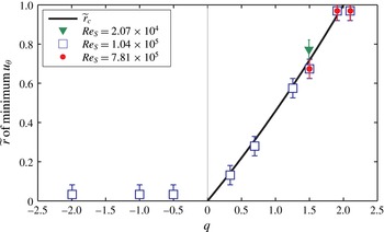
. Hence, we can quantify the radial position of the transition region by finding the radial positions for which the azimuthal velocity profiles
 $u_{{\it\theta}}(r)$
are at their minimum. They are shown in figure 7. In the quasi-Keplerian regime, we find that the position of the minimum velocity corresponds very well with
 $\widetilde{r}_{c}$
in (4.6), giving merit to the approximate profiles of (4.4). Outside of the quasi-Keplerian regime, the position of the minimum is located at the inner cylinder for
 $q<0$
, and at the outer cylinder for
 $q>2$
.
Radial positions of the minimum in the azimuthal velocity
 $u_{{\it\theta}}$
as a function of
 $q$
(
 $x$
-axis) and
 $\mathit{Re}_{S}$
(different symbols). In the quasi-Keplerian regime,
 $\widetilde{r}_{c}$
from (4.6) is shown for comparison (solid line).

The approximately flat angular momentum profile in the inner region, when away from the Rayleigh line where the laminar Taylor–Couette profile is flat, indicates that the angular momentum is well mixed with advection-dominated transport in the radial direction. In contrast, there is probably little radial angular momentum transport by advection or diffusion in the outer region as the profile is close to solid-body at
 ${\it\Omega}_{o}$
. A large amount of angular momentum is transported radially from the inner cylinder based on the torque measurements from the similar Maryland experiment (Paoletti & Lathrop Reference Paoletti and Lathrop2011) and the upcoming analysis of § 4.3. The large amount of angular momentum transported off the inner cylinder and mixed in the inner region has to go somewhere, but the outer region, if present, is probably not transporting much angular momentum. Then, when an outer region is present such as when
 $q<2$
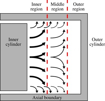
far from the Rayleigh line, most of the angular momentum must be transported axially to the axial boundaries in the inner and possibly middle regions, as shown schematically in figure 8. As
 $q$
increases at fixed
 $\mathit{Re}_{S}$
towards the Rayleigh line, the outer region disappears and an increasing fraction of the angular momentum can be transported to the outer cylinder through the middle region instead of being transported to the axial boundaries. For
 $q\geqslant 2$
, there is no middle region and a boundary layer forms close to the outer cylinder that steepens with increasing
 $q$
(van Gils et al.
Reference van Gils, Huisman, Grossmann, Sun and Lohse2012), indicating that an increasing fraction of the angular momentum is transported to the outer cylinder instead of to the axial boundaries. Finally, nearly all of the angular momentum is transported to the outer cylinder.
Schematic drawing of the angular momentum transport in the quasi-Keplerian regime when the axial boundaries are attached to the outer cylinder. Red dashed lines denote the boundaries between the inner, middle and outer flow regions. Black arrows denote the transport of angular momentum. The radius and aspect ratios (
 ${\it\eta}$
and
 ${\it\Gamma}$
) have been changed for visual clarity. Angular momentum is transported radially off the inner cylinder and then transported axially to the axial boundaries in the inner and middle regions.

These features are also seen in wide-gap low-aspect-ratio experiments. Using dye injection from the inner cylinder, Dunst (Reference Dunst1972) found a well-mixed inner region and a quiescent outer region with poor mixing. In figure 9, the angular velocity and the specific angular momentum profiles for
 $q\approx 1.9$
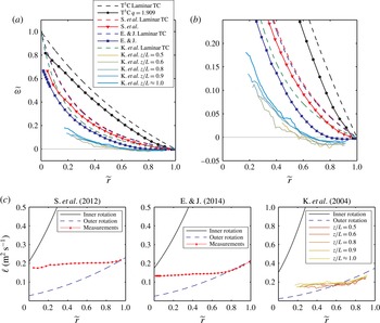
from Kageyama et al. (Reference Kageyama, Ji, Goodman, Chen and Shoshan2004), Schartman et al. (Reference Schartman, Ji, Burin and Goodman2012) and Edlund & Ji (Reference Edlund and Ji2014) are compared with each other and with the results from our apparatus. They all deviate from the laminar Taylor–Couette profile and show the same three regions with a relatively flat
 $\ell$
close to the inner cylinder and rotate close to
 ${\it\Omega}_{o}$
close to the outer cylinder. However, the relatively flat
 $\ell$
inner region is offset downward from the specific angular momentum on the inner cylinder, indicating the presence of a boundary layer on the inner cylinder more significant than in our experiment. The experiments of Kageyama et al. (Reference Kageyama, Ji, Goodman, Chen and Shoshan2004) and possibly Edlund & Ji (Reference Edlund and Ji2014) also exhibit flow sub-rotation (
 ${\it\omega}<{\it\Omega}_{o}<{\it\Omega}_{i}$
) in the middle and outer regions. The axial transport of angular momentum and the presence of three regions in the quasi-Keplerian azimuthal velocity profiles appear to be more general than just occurring in our specific apparatus with its geometry and ranges of
 $\mathit{Re}_{S}$
and
 $q$
, although the strength of the boundary layer on the inner cylinder appears to depend on
 ${\it\eta}$
and/or
 ${\it\Gamma}$
.
Comparison of the azimuthal velocimetry for
 $q\approx 1.9$
between different experiments. This includes our experiment (
 $\text{T}^{3}\text{C}$
) with
 ${\it\eta}=0.716$
at
 $q=1.909$
and
 $\mathit{Re}_{S}=7.82\times 10^{5}$
, Schartman et al. (Reference Schartman, Ji, Burin and Goodman2012) with
 ${\it\eta}=0.348$
at
 $q=1.908$
and
 $\mathit{Re}_{S}=5.05\times 10^{5}$
, Edlund & Ji (Reference Edlund and Ji2014) with
 ${\it\eta}=0.340$
at
 $q=1.803$
and
 $\mathit{Re}_{S}=4.34\times 10^{5}$
, and Kageyama et al. (Reference Kageyama, Ji, Goodman, Chen and Shoshan2004) with
 ${\it\eta}=0.255$
at
 $q=1.896$
and
 $\mathit{Re}_{S}=1.30\times 10^{6}$
. The profiles for Schartman et al. (Reference Schartman, Ji, Burin and Goodman2012) and Edlund & Ji (Reference Edlund and Ji2014) were constructed by extracting velocities from their figures (6 and 2 respectively). Kageyama et al. (Reference Kageyama, Ji, Goodman, Chen and Shoshan2004) performed velocimetry at five different axial heights. Profiles for Kageyama et al. (Reference Kageyama, Ji, Goodman, Chen and Shoshan2004) were constructed by splitting the range
 $\widetilde{r}\in [0,\,1]$
into bins of width 0.02 and averaging the
 ${\it\omega}$
within each bin. Normalized angular velocity
 $\widetilde{{\it\omega}}$
profiles are compared (a) at full scale and (b) expanded around
 $\widetilde{{\it\omega}}=0$
using the same symbols to emphasize the parts of the profiles close to rotation at
 ${\it\Omega}_{o}$
. Dashed lines are the laminar Taylor–Couette profiles for each experiment. (c) The specific angular momentum (
 $\ell =r^{2}{\it\omega}$
) profiles for each experiment side by side with the same horizontal axes and with vertical axes in the same units. The solid black line (——) and dashed blue line (– – –) are the specific angular momentum profiles for
 ${\it\omega}(\widetilde{r})={\it\Omega}_{i}$
and
 ${\it\omega}(\widetilde{r})={\it\Omega}_{o}$
respectively.

4.3. Torque on the inner cylinder
The velocity gradients near the inner cylinder were larger than in laminar Taylor–Couette flow, as the
 $\widetilde{{\it\omega}}$
values at the point closest to the inner cylinder in figures 3 and 5(a) are below that of the laminar Taylor–Couette profile. This steepness means that the torque on the inner cylinder must be larger than in laminar Taylor–Couette flow. If boundary layers were present, the profiles would be even steeper at the inner cylinder, and thus the torques even larger.
The azimuthal shear stress, when averaged azimuthally, is
 ${\it\tau}=-{\it\rho}{\it\nu}r(\partial {\it\omega}/\partial r)$
, where
 ${\it\rho}$
is the fluid density (see p. 48, Landau & Lifshitz Reference Landau and Lifshitz1987). The torque
 $T$
on a cylinder of radius
 $r$
from just the shear stress is
 $T_{{\it\nu}}=2{\rm\pi}r^{2}L{\it\tau}$
, which in terms of the angular velocity is
 $$\begin{eqnarray}T_{{\it\nu}}=-2{\rm\pi}{\it\rho}{\it\nu}Lr^{3}\frac{\partial {\it\omega}}{\partial r}.\end{eqnarray}$$
As laminar Taylor–Couette flow has no Reynolds stresses and
 ${\it\omega}$
is uniform over a cylinder of radius
 $r$
from (1.4), the total laminar Taylor–Couette torque is
 $$\begin{eqnarray}T_{lam}=\frac{2{\rm\pi}{\it\rho}{\it\nu}^{2}L{\it\eta}}{(1-{\it\eta})^{2}}\mathit{Re}_{S}\,\text{sign}(\mathit{Re}_{i}-{\it\eta}\mathit{Re}_{o}).\end{eqnarray}$$
Assuming a turbulent boundary layer, the thickness
 $y_{0}$
of the viscous sublayer on the inner cylinder is
 $y_{0}=({\it\nu}/u^{\ast })y_{0}^{+}$
, where
 $u^{\ast }=\sqrt{|{\it\tau}|/{\it\rho}}$
is the friction velocity,
 ${\it\rho}$
is the fluid density and
 $y_{0}^{+}$
is the sublayer thickness in dimensionless units (Schlichting Reference Schlichting1979). From measurements in our apparatus for pure inner cylinder rotation at comparable
 $\mathit{Re}_{S}$
,
 $y_{0}^{+}$
is in the range of 5–10 (Huisman et al.
Reference Huisman, Scharnowski, Cierpka, Kähler, Lohse and Sun2013). Then, for
 $\mathit{Re}_{S}=10^{5}$
, we get
 $y_{0}\leqslant 2~\text{mm}$
since
 $T\geqslant T_{lam}$
and
 $y_{0}^{+}\leqslant 10$
. Since
 $r-r_{i}=2.6~\text{mm}$
was the point closest to the inner cylinder where the flow velocity was resolved, our azimuthal velocimetry did not extend into the viscous sublayer. Due to not resolving the viscous sublayer, the torque in our apparatus cannot be obtained from the velocity profiles, meaning that direct comparisons cannot be made with the torque measurements of Paoletti & Lathrop (Reference Paoletti and Lathrop2011) from the Maryland experiment with near identical geometry. However, lower bounds on the torque can be obtained because the azimuthal profiles can give the shear stress, instead of both the shear and Reynolds stresses.
To obtain the lower bound for the torque on the inner cylinder,
 $\partial {\it\omega}/\partial r$
was obtained from the difference between
 ${\it\omega}$
at the point closest to the inner cylinder (
 $r-r_{i}=2.6~\text{mm}$
which is
 $\widetilde{r}=0.033$
) and
 ${\it\Omega}_{i}$
at the inner cylinder. It must be noted that the velocity profile was taken at the axial height of one of the small separations in the inner cylinder, which was 2.5 mm thick, and therefore the gradients in
 ${\it\omega}$
we calculate might be perturbed compared with other axial heights due to the vicinity to the separation.
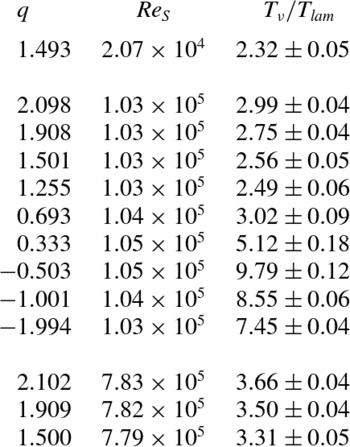
The torque lower bounds are listed in table 2. The lower bounds were all larger than the laminar Taylor–Couette torque, which supports the
 $|T/T_{lam}|\gg 1$
result of Paoletti & Lathrop (Reference Paoletti and Lathrop2011) from the similar Maryland experiment in both regimes for
 $\mathit{Re}_{S}>3.5\times 10^{5}$
. The measurements in this paper extend this result of Paoletti & Lathrop (Reference Paoletti and Lathrop2011) towards solid-body rotation in both regimes.
The ratios of the lower bounds of the torque on the inner cylinder
 $T_{{\it\nu}}$
to the laminar Taylor–Couette torque
 $T_{lam}$
for each set of measurements, ordered by
 $\mathit{Re}_{S}$
and then by
 $q$
.

For the quasi-Keplerian regime, we can use the approximate flatness of the specific angular momentum profile in the inner region to make an analytical approximate torque lower bound. Treating the inner region as having a flat specific angular momentum profile from the inner cylinder with no boundary layer as in (4.4), the ratio of the torque lower bound
 $T_{{\it\nu},flat}$
to the laminar Taylor–Couette torque is
 $$\begin{eqnarray}\frac{T_{{\it\nu},flat}}{T_{lam}}=\frac{1-{\it\eta}^{2}}{1-{\it\eta}^{q}}\quad \text{for}~0<q\leqslant 2.\end{eqnarray}$$
The ratio is always larger than one, approaching one at
 $q=2$
. It diverges as
 $q\rightarrow 0$
, which is due to the width of the inner region shrinking towards zero since
 $r_{c}\rightarrow r_{i}$
in (4.5). The decrease in
 $r_{c}$
means that
 ${\it\omega}$
changes from
 ${\it\Omega}_{i}$
to
 ${\it\Omega}_{o}$
over an ever smaller radial distance, giving a sharper gradient of
 ${\it\omega}$
in the inner region, which becomes infinite as
 $q\rightarrow 0$
. However, if the inner region of a flat angular momentum profile disappears entirely as
 $q\rightarrow 0$
at a given
 $\mathit{Re}_{S}$
, then this lower bound may no longer hold. For
 $\mathit{Re}_{S}=1.04\times 10^{5}$
, the inner region might be close to disappearing by
 $q=0.333$
based on the angular momentum profiles in figure 4. As the middle region shrinks with increasing
 $\mathit{Re}_{S}$
(figure 5
b), the
 $q$
at which the inner region might disappear decreases with increasing
 $\mathit{Re}_{S}$
.
The torque lower bounds can be compared with the torque scaling that Paoletti et al. (Reference Paoletti, van Gils, Dubrulle, Sun, Lohse and Lathrop2012) fit to the Maryland torque measurements in the Rayleigh-stable and -unstable regimes (Paoletti & Lathrop Reference Paoletti and Lathrop2011) and the torque measurements on the apparatus presented in this paper in the unstable regime (van Gils et al.
Reference van Gils, Huisman, Bruggert, Sun and Lohse2011b
). The scaling was for the ratio of the torque on the inner cylinder to the torque
 $T_{+\infty }$
for pure inner rotation (
 $q=+\infty$
) at the same
 $\mathit{Re}_{S}$
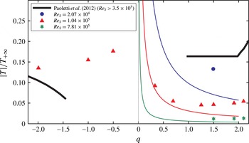
, which in this paper was obtained from torque measurements in the very similar Maryland experiment (equation (9) in Lathrop, Fineberg & Swinney Reference Lathrop, Fineberg and Swinney1992). The lower bounds are compared with the torque scaling
 $\mathit{Re}_{S}>3.5\times 10^{5}$
(equation (12) in Paoletti et al.
Reference Paoletti, van Gils, Dubrulle, Sun, Lohse and Lathrop2012) in figure 10.
Comparison of inner cylinder torque lower bounds calculated at
 $z/L=0.209$
with the torques measured by Paoletti et al. (Reference Paoletti, van Gils, Dubrulle, Sun, Lohse and Lathrop2012). Torques are normalized by the torque for pure inner rotation at the same
 $\mathit{Re}_{S}$
. The scaling of Paoletti et al. (Reference Paoletti, van Gils, Dubrulle, Sun, Lohse and Lathrop2012) for
 $\mathit{Re}_{S}>3.5\times 10^{5}$
is the thick black solid line. The torque ratio lower bounds obtained from the velocity profiles are the symbols, coded by
 $\mathit{Re}_{S}$
. The lower bound torques from the quasi-Keplerian flat inner angular momentum profile approximation in (4.9) for each
 $\mathit{Re}_{S}$
are the thin solid lines with the same colours as the symbols, which increase with decreasing
 $\mathit{Re}_{S}$
. The error bars are smaller than the symbols.

As the torque ratios must be positive, the torque scaling must start curving upwards on the sub-rotating regime side when approaching solid-body rotation at some
 $q>-1.5$
to avoid crossing zero. The three sub-rotating regime torque lower bounds for
 $\mathit{Re}_{S}=1.04\times 10^{5}$
give
 $|T|/T_{+\infty }$
values that are larger than those for
 $\mathit{Re}_{S}>3.5\times 10^{5}$
(Paoletti et al.
Reference Paoletti, van Gils, Dubrulle, Sun, Lohse and Lathrop2012). Thus, the
 $|T|/T_{+\infty }$
scaling of Paoletti et al. (Reference Paoletti, van Gils, Dubrulle, Sun, Lohse and Lathrop2012) must increase if extended to
 $\mathit{Re}_{S}=1.04\times 10^{5}$
.
On the quasi-Keplerian side, comparisons can be made between our measurements at
 $\mathit{Re}_{S}=7.81\times 10^{5}$
and those of Paoletti et al. (Reference Paoletti, van Gils, Dubrulle, Sun, Lohse and Lathrop2012) for
 $\mathit{Re}_{S}>3.5\times 10^{5}$
. Our
 $|T|/T_{+\infty }$
lower bounds from both the measured velocity profiles and the flat inner region approximation from (4.9) are considerably smaller than those of Paoletti et al. (Reference Paoletti, van Gils, Dubrulle, Sun, Lohse and Lathrop2012). As our lower bounds only considered shear stress (diffusion), the difference in torques on the inner cylinder must be due to Reynolds stresses (advection) in the region of
 $\widetilde{r}\leqslant 0.033$
. The divergence of the torque lower bound for the flat inner region angular momentum approximation as
 $q\rightarrow 0$
suggests that the flat quasi-Keplerian
 $|T|/T_{+\infty }$
scaling of Paoletti et al. (Reference Paoletti, van Gils, Dubrulle, Sun, Lohse and Lathrop2012) will deviate from being flat if extended to
 $q<1$
, unless the inner region disappears or is distorted close to solid-body rotation.
5. Summary and conclusions
In summary, azimuthal velocity profiles were obtained for several Rayleigh-stable (and one unstable) cylinder rotation rate ratios for the ranges
 $2.098\geqslant q\geqslant 0.333$
and
 $-1.994\leqslant q\leqslant -0.503$
. They were all carried out for
 $\mathit{Re}_{S}=1.04\times 10^{5}$
, a few configurations at
 $\mathit{Re}_{S}=7.81\times 10^{5}$
, and just the Keplerian configuration also at
 $\mathit{Re}_{S}=2.07\times 10^{4}$
. For all values of
 $q$
, the profiles deviate from the laminar Taylor–Couette profile. The deviation increases as solid-body rotation is approached (
 $q\rightarrow 0$
) at fixed non-zero
 $\mathit{Re}_{S}$
. The deviation consists of a steepening of the normalized angular velocity
 $\widetilde{{\it\omega}}$
profile close to the inner cylinder for all
 $q$
, and the flow in the outer parts of the gap approaching solid-body rotation with the outer cylinder and attached axial boundaries for the quasi-Keplerian regime.
For the sub-rotating regime, the flow exhibits super-rotation compared with both cylinders (
 ${\it\omega}>{\it\Omega}_{o}>{\it\Omega}_{i}$
), except close to the inner cylinder. As solid-body rotation is approached at fixed
 $\mathit{Re}_{S}=1.04\times 10^{5}$
, the strength of the super-rotation increases, reaching 6 % of
 ${\it\Omega}_{o}-{\it\Omega}_{i}$
for
 $q=-0.503$
, and the radial positions of the maximum of super-rotation and where the flow switches from
 ${\it\Omega}_{i}<{\it\omega}<{\it\Omega}_{o}$
to super-rotation move closer to the inner cylinder. The flow super-rotation must be sustained by inward angular momentum transport from the outer cylinder or axial boundaries. To the best of our knowledge, flow super-rotation for
 $q<0$
has not been previously observed in the literature. This includes pure outer rotation (
 $q=-\infty$
) in our apparatus (van Gils et al.
Reference van Gils, Bruggert, Lathrop, Sun and Lohse2011a
) and in those of Wendt (Reference Wendt1933), Taylor (Reference Taylor1936b
) and Burin & Czarnocki (Reference Burin and Czarnocki2012).
For the quasi-Keplerian regime, the specific angular momentum profiles show that the flow can be split into three regions across the gap: an inner region where the angular momentum profile is approximately flat, an outer region where the flow is close to solid-body rotation at
 ${\it\Omega}_{o}$
, and a middle transition region between the two. Starting near the Rayleigh line, the middle and outer regions are almost non-existent, and then as solid-body rotation is approached at fixed non-zero
 $\mathit{Re}_{S}$
, the inner region shrinks while the outer region grows until the inner region is almost non-existent at
 $q=0.333$
. As
 $\mathit{Re}_{S}$
is increased, the middle region shrinks. We speculate that as
 $\mathit{Re}_{S}\rightarrow \infty$
, the middle region will disappear and the profile will converge towards (4.4) (independently derived from dye injection observations by Dunst Reference Dunst1972). This model profile is a good approximation by
 $\mathit{Re}_{S}=7.81\times 10^{5}$
. The outer region, if present, probably transports little angular momentum, meaning that almost all of the angular momentum is transported to the axial boundaries. Work is still needed to check how the mixing is achieved in the inner region and whether the inner region is turbulent. One must also determine the exact nature of the flow in the middle and outer regions, and see whether the region pattern is found for other
 ${\it\eta}$
and
 ${\it\Gamma}$
. Measurement of the separate torques on the inner cylinder, outer cylinder and axial boundaries, or performance of very-high-resolution particle image velocimetry as Huisman et al. (Reference Huisman, van Gils, Grossmann, Sun and Lohse2012a
) did for pure inner rotation on the same apparatus would be good ways to determine what fraction of the angular momentum goes to the axial boundaries versus the outer cylinder and elucidate the axial transport mechanism. We do not see flow sub-rotation in our experiment except possibly for
 $q=0.693$
and 0.333, but
 $\widetilde{{\it\omega}}\approx 0$
within the measurement precision at those
 $q$
. However, Kageyama et al. (Reference Kageyama, Ji, Goodman, Chen and Shoshan2004) and possibly Edlund & Ji (Reference Edlund and Ji2014) found sub-rotating flow for
 $q>0$
.
The slope of the angular velocity profile at the inner cylinder is steeper than in laminar Taylor–Couette flow for both the sub-rotating and the quasi-Keplerian regimes. Therefore, the torque required to rotate the inner cylinder must be larger than the laminar Taylor–Couette value, which supports the super-laminar torque measurements from the geometrically similar Maryland experiment (Paoletti & Lathrop Reference Paoletti and Lathrop2011). Due to not resolving the viscous sublayer on the inner cylinder, only lower bounds for the torque on the inner cylinder could be obtained via a viscous stress calculation. The
 $|T|/T_{+\infty }$
lower bounds from the velocity measurements and the approximate asymptotic profile were compared with the
 $|T|/T_{+\infty }$
scaling found by Paoletti et al. (Reference Paoletti, van Gils, Dubrulle, Sun, Lohse and Lathrop2012) for
 $\mathit{Re}_{S}>3.5\times 10^{5}$
. In the sub-rotating regime, their
 $|T|/T_{+\infty }$
scaling needs to be increased if extended to
 $\mathit{Re}_{S}=10^{5}$
or towards solid-body rotation. In the quasi-Keplerian regime, the comparison also shows that the bulk of the transport of angular momentum off the inner cylinder is by Reynolds stresses (advection), and the
 $|T|/T_{+\infty }$
scaling of Paoletti et al. (Reference Paoletti, van Gils, Dubrulle, Sun, Lohse and Lathrop2012) may require modification as
 $q\rightarrow 0$
.
Our velocity profiles provide experimental confirmation of the expectation that the Ekman pumping from the axial boundaries was what destabilized the flow in the Maryland experiment, which has a nearly identical geometry to our apparatus, in the Rayleigh-stable regime, causing large super-laminar torques on the inner cylinder (Balbus Reference Balbus2011; Avila Reference Avila2012; Ji & Balbus Reference Ji and Balbus2013; Edlund & Ji Reference Edlund and Ji2014). This work, combined with the work of Avila (Reference Avila2012), Schartman et al. (Reference Schartman, Ji, Burin and Goodman2012) and Edlund & Ji (Reference Edlund and Ji2014), resolves the apparent discrepancy between the approximately laminar Taylor–Couette angular momentum transport in the wide-gap low-aspect-ratio experiments with axial boundaries split into rings rotating at speeds intermediate to those of the cylinders, such as the Princeton MRI and HTX experiments (Ji et al. Reference Ji, Burin, Schartman and Goodman2006; Schartman et al. Reference Schartman, Ji, Burin and Goodman2012; Edlund & Ji Reference Edlund and Ji2014), and large super-laminar angular momentum transport in the medium-gap higher-aspect-ratio Maryland experiment with axial boundaries attached to the outer cylinder (Paoletti & Lathrop Reference Paoletti and Lathrop2011). Moreover, we found that the Ekman pumping from the axial boundaries does more than just destabilize the flow in the Rayleigh-stable regime when the axial boundaries are attached to the outer cylinder. In the quasi-Keplerian regime, it causes the flow to be split radially into three regions and nearly all of the angular momentum to be transported to the axial boundaries instead of the outer cylinder when an outer region is present. The Ekman pumping essentially causes the axial boundaries to become the primary sink of angular momentum. In the sub-rotating regime, we discovered flow super-rotation, which is also probably due to the Ekman pumping.
Astrophysical accretion disks have open axial boundaries, which do not cause Ekman pumping, and are thought or assumed to have primarily radial transport of angular momentum (Zeldovich Reference Zeldovich1981; Richard & Zahn Reference Richard and Zahn1999; Richard Reference Richard2001; Dubrulle et al.
Reference Dubrulle, Dauchot, Daviaud, Longaretti, Richard and Zahn2005a
; Ji & Balbus Reference Ji and Balbus2013; Ostilla-Mónico et al.
Reference Ostilla-Mónico, Verzicco, Grossmann and Lohse2014). Due to the strong Ekman pumping effects, including the primarily axial transport of angular momentum, Taylor–Couette flow with an aspect ratio up to
 ${\it\Gamma}\sim 10$
with no-slip axial boundaries attached to the outer cylinder is an imperfect model of accretion disks, especially with regard to stability. Ideally, one would like to have axial boundaries that are free-slip or rotate at different rates along their radius such that they match the mean rotation rate of what the flow would be in the absence of axial boundaries, which may not be the laminar Taylor–Couette profile.
There are practical options available for experimental Taylor–Couette flow to mitigate the Ekman pumping and make a better model of accretion disks. One practical way is to make an experiment where the aspect ratio is great enough that the axial transport mechanism of the angular momentum saturates and Ekman pumping can no longer directly affect the flow near midheight. However, tall experiments are difficult to handle and expensive to make, and work would be needed to ascertain whether indirect effects would still be a problem. Another way, which has been followed by the Princeton group (Ji et al. Reference Ji, Burin, Schartman and Goodman2006; Schartman et al. Reference Schartman, Ji, Burin and Goodman2012; Edlund & Ji Reference Edlund and Ji2014), is to split the axial boundaries into rings that are rotated at speeds intermediate to those of the cylinders. This reduces the strength of the Ekman pumping as well as better confining it to the axial boundaries. Implementation of the independently rotating rings is difficult and there is still Ekman pumping due to having only a finite number of independently rotating rings. If the working fluid is a liquid, the top boundary can be made into an open boundary by having gas above it, reducing the Ekman pumping at the top by three orders of magnitude in the case of water and air, although it does introduce the problem of gravity waves on the top surface. For the velocities that are used in the present experiments, air could be entrained by these waves. Similarly, density-mismatched fluids such as mercury and water or stratification (e.g. salt solutions) can be used on the bottom boundary to confine the Ekman circulation near the bottom by reducing axial circulation, although this also introduces the problem of gravity waves and mixing which would destroy the stratification. In order to accurately represent an accretion disk, one probably has to combine more than one of these methods.
Acknowledgements
We would like to acknowledge helpful discussions and advice from D. P. M. van Gils, S. Grossmann, R. Ostilla-Mónico, D. S. Zimmerman, E. M. Edlund and H. Ji. We thank H. Ji for providing us with the velocimetry data from Kageyama et al. (Reference Kageyama, Ji, Goodman, Chen and Shoshan2004). We also acknowledge work and advice from the technicians G.-W. Bruggert, M. Bos and B. Benschop, and financial support from the Technology Foundation STW of The Netherlands from an ERC Advanced Grant and the National Science Foundation of the USA (grant no. NSF-DMR 0906109).
Supplementary data
Supplementary data are available at http://dx.doi.org/10.1017/jfm.2015.275.