

Introduction
Yield maps are a powerful tool when it comes to make informed management decisions with regard to upcoming crop productions. However, yield datasets can contain a large amount of defective data (Griffin et al., Reference Griffin, Dobbins, Vyn, Florax and Lowenberg-DeBoer2008). To robustify these datasets, multiple works have reported sequential screening processes to remove most of the sources of errors (Simbahan et al., Reference Simbahan, Dobermann and Ping2004; Sudduth et al., Reference Sudduth and Drummond2007). From a general perspective, these authors have validated their approach because the yield distribution and spatial structure were significantly improved after removing these defective observations. Even though this validation seems appropriate, it is not possible to evaluate objectively an approach towards a specific type of error or even to compare multiple filtering methods. Experts are sometimes involved in the validation step but this kind of validation is relatively rare. Furthermore, it is relevant to wonder whether an expert is truly able to identify all the errors in a dataset. As crops cannot be harvested twice, it is difficult to make use of ground-truth measurements to validate some proposed methodologies.
Synthetic datasets are widely used in many application domains to overcome these limitations (Breunig et al., Reference Breunig, Kriegel, Ng and Sander2000). From a general perspective, algorithms are often initially validated on synthetic datasets that include noise, and are then, applied on real datasets. Since the main sources of errors in yield datasets are known, it is conceivable to integrate these errors in synthetic datasets to simulate real yield datasets. Authors essentially focus on lowering (i) the number of false positives (swamping effect), i.e. to avoid wrongly classifying an observation as a defective observation or (ii) the number of false negatives (masking effect), i.e. defective data are not identified as such (Ben-Gal, Reference Ben-Gal2005). This work proposes a methodology to produce simulated yield datasets. So far, the efficiency of yield filtering approaches has never been assessed objectively which makes users unable to choose an appropriate method when it comes to correct yield datasets. These simulated datasets will help evaluate and compare yield post-processing methods.
Material and methods
The simulation process consisted in two major steps: (i) the creation of spatially correlated datasets and (ii) the addition of known yield sources of errors to these datasets. These sources of errors can be categorized into four major groups: (i) the harvesting dynamics of the combine harvester, (ii) the continuous measurements of yield and moisture, (iii) the accuracy of the positioning system and, (iv) the harvester operator (Lyle et al., Reference Lyle, Bryan and Ostendorf2013). Fields were created with geometric shapes, i.e. square or rectangles, to facilitate the construction of harvest passes. These passes were considered mostly harvested in straight lines. Some specific harvest patterns were added during the simulation, e.g. harvest turns, but adding complex harvest patterns inside the fields was not considered in this work. Fields were delimitated by headlands, modelled by straight lines perpendicular to harvest passes. The methodology was developed using the R statistical environment (R Core Team, Vienna, Austria).
Modelling the sources of errors in spatially correlated datasets
First step of the simulation process was to create spatially correlated datasets as yield datasets generally exhibit some spatial autocorrelation to a greater or lesser extent (Sudduth et al., 2007). Gaussian random fields were simulated via the sequential simulation algorithm in the gstat package (Bivand et al., 2013). Main sources of errors were modelled and added to the previously defined spatially correlated datasets. Let y i (s,t) be the yield value of an observation i located at a spatial position s and acquired at a time t. For each error e to apply to an observation i, a function f e will be applied to i and will result in the transformation of y i (s,t) into y’ i (s’,t’) as follows:
 $$f_{e} \,\colon\,y_{i} (s,t) \to y{'}\!_{i} (s{'} ,t{'} )$$
Note that y’ i , s’ and t’ are not necessarily different from y i , s and t respectively. All the errors were added in a specific order that follows the description of the sources of errors. Only the simulation of the main sources of errors will be detailed.
Speed changes
Speed changes are a relatively common phenomenon during harvest. They induce (i) an increase or decrease in the number of total observations given the constant sampling frequency of the sensor and (ii) yield variations. This source of error can be modelled by the following function
 $f_{{speed}} \,\colon\,y_{i} \left( {s,t} \right) \to y{'}\!_{i}\, (s{'} ,t)$
. The model will consist in two steps; the transformation of y
i
(s,t) into y
i
(s’,t) and then that of y
i
(s’,t) into y’
i
(s’,t).
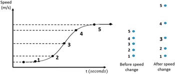
Step 1: y i (s,t) into y i (s’,t). Speed changes are assumed graduate, to a lesser or greater extent, and therefore were chosen to be modelled by sigmoid functions (Fig. 1). By varying the shape of the sigmoid, a large range of speed change dynamics can be simulated. Considering a constant sampling frequency, speed changes can be simply understood as a change in distance between consecutive observations (Fig. 1, right).
Simulation of an increase in speed (left) and the corresponding shift in distance between consecutive points (right).

Step 2: y i (s’,t) into y’ i (s’,t). When speed strongly decreases, yield values significantly increase because the harvest area (distance travelled by cutting width) is largely decreased while grain flow remains constant (Eq. 2). The distance between two observations necessarily depends on the sampling frequency and the speed of the machine. Reasoning is reverse when speed increases.
 $$Yield\,\, {\equals}\, \, {{Grain\,flow} \over {Distance\,travelled{\times}Cutting\,width}}$$
The stronger the speed change, the stronger the yield variation. As speed stabilizes, grain flow gets stable too and yield values are back to normal. As a consequence, to affect a new yield value to an observation i during a speed change, there is a need to take into account the speed changes that occurred before this record i. For each harvest pass, the yield transformation is defined as follows:
 $$y_{i}{{\rm '}} \left( {s{{\rm '}} ,t} \right)_{k} \, {\equals}\, y_{i} \left( {s{{\rm '}} ,t} \right)_{k} {\plus}{\rm }\mathop{\sum}\nolimits_{j\,\, {\equals}\, \,1}^{j\,\, {\equals}\, \,i} {{{Diff(j)} \over {2^{{i{\minus}j}} }}} \,{\rm }\forall {\rm }\,the\,{\rm }harvest\,{\rm }pass{\rm }k$$
where k stands for the k th pass.
The factor 2 i−j makes sure that a speed change occurring during the acquisition of observation j (j<i) has more impact on the yield value of observation i when both observations are acquired simultaneously than when they are very spaced. This factor can be seen as an attenuation factor. Diff(j) takes into account the intensity of speed change between an observation j and the observation acquired previously j−1 as follows:
 $$Diff(\,j)\, {\equals}\, \left( {{{{\rm }g\left( t \right)_{j} \,{\minus}\,g\left( t \right)_{{j{\minus}1}} } \over {g\left( t \right)_{{j{\minus}1}} }}} \right){\times}y_{j} \left( {s{{\rm '}} ,t} \right)_{k} $$
where g(t)
j
and g(t)
j−1 are the speeds of the combine at observation j and j−1. Note that when speed is constant at j and j−1, Diff(j) equals zero and
 $y{'}\!_{i} (s{'} ,t)$
equals y
i
(s’,t).
Low cutting width
Unknown crop width entering the header is a critical issue in yield data processing. Overestimated swath width (SW) will result in yield values significantly lower than expected (Eq. 2). Passes harvested with a low cutting width are located at a distance inferior to the full width of the cutting bar from previously harvested passes.
Simulation:
 $f_{{width}} \,\colon\,y_{i} \left( {s,t} \right) \to y{'}\!_{i} \arrow (s{'} ,t)$
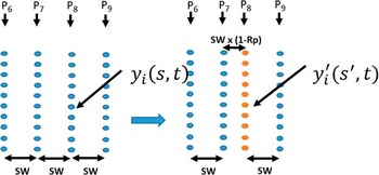
. Assume ten passes Pk (k=1 to 10) harvested from P1 to P10 from which one has been randomly selected and considered to be harvested with a low cutting width (P8 in this case). A random number R
P
, ranging between 0 and 1, defines the amount of SW that is used to harvest P8 (Fig. 2). Hence, yield values in P8 are transformed using the following equation:
 $$y{'}\!_{i} \left( {s,t} \right)\,\, {\equals}\, \,y_{i} \left( {s,t} \right){\times}R_{P} $$
Simulating a pass harvested with a low cutting width. P8 has been harvested with a non-full swath width and was brought closer to the previously harvest pass P7. The distance between P8 and P9 is still equal to SW.

From a spatial perspective, all
 $y{'}\!_{i} \left( {s,t} \right)$
observations in P
8
are shifted towards the pass previously harvested, i.e. P7, by a distance d
width equal to SW × (1−RP) as follows:
 $$y{'}\!_{i} \left( {s{{\rm '}} ,t} \right)\,\, {\equals}\, \,y{'}\!_{i} (s\,{\minus}\,d_{{width}} ,{\rm }t)$$
Note that the reduced cutting width is applied to a full harvest pass.
Time delays
Lag time delay was not modelled during the simulation. It was considered that lag time had already been accounted for, which means that yield observations had been shifted accordingly to meet their real neighbourhood. Filling and emptying times, respectively start and end pass delays, are responsible for low yield estimates when the combine harvester enters or leaves a pass.
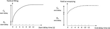
Simulation: f delay :y i (s,t)→y i ’(s,t). Grain flow dynamics near start and end rows have been reported multiples times (Lyle et al., Reference Lyle, Bryan and Ostendorf2013; Simbahan et al., Reference Simbahan, Dobermann and Ping2004). Grain flow increases until reaching a plateau, the permanent regime, and then decreases again as the combines leaves the harvest pass (Fig. 3). Note that the x-axis is plotted backwards for end delay times. Grain flow dynamics at both start and end rows were then modelled by similar functions, more specifically with spherical functions. These functions are used to weigh the yield values at the beginning and end of rows as follows:
 $$y{'}\!_{i} \left( {s,t} \right)\,\, {\equals}\, \,y_{i} \left( {s,t} \right){\times}{{y_{i} \left( {s,t} \right)} \over {C_{k} {\plus}B_{k} }}$$
where Bk is the yield intercept and Ck is the range of yield values during filling or emptying times. Note that the shape of the curves is slightly different (Figure 3). Indeed, when looking at the shape of previously reported grain flow dynamics, yield is more underestimated when the combine enters the crop than when it leaves (Blackmore, 1999; Simbahan et al., Reference Simbahan, Dobermann and Ping2004).
Simulating grain flow dynamics at start (left) and end rows (right).

Estimating simulation parameters from real yield datasets
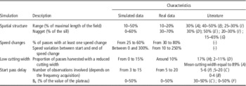
Simulation parameters (range and bounds) were set after a review of the literature and an evaluation of yield maps from five fields located near Evreux, north-west of France (Table 1). For these five fields, yield measurements were obtained with a grain flow sensor mounted on a combine harvester (New Holland, Turin, Italy). Passes were mostly harvested in straight lines. Cutting width was 9 meters for the five fields. The literature and these yield maps were analysed to extract the major characteristics of each known sources of error to make sure that simulated datasets were reliable. When the information was not available in the literature, only the five fields under study were used to estimate the corresponding parameters. Once yield datasets were simulated, three published filtering methods (Simbahan et al., Reference Simbahan, Dobermann and Ping2004; Sudduth et al., 2007, Sun et al., Reference Sun, Whelan, McBratney and Minasny2013) were applied on these simulations to determine whether the amount of defective observations detected was consistent with that reported in the literature. Twenty simulations were run and submitted to the filtering algorithms.
Yield spatial structures and amounts of errors found in real datasets and literature, and those used during simulations. Note that all characteristics are not presented. (-) indicates that clear characteristics were not found

A: Drummond et al. (Reference Drummond, Fraisse and Sudduth1999) – B: Griffin et al. (Reference Griffin, Dobbins, Vyn, Florax and Lowenberg-DeBoer2008) – C: Lyle et al. (Reference Lyle, Bryan and Ostendorf2013) - D: Molin et al. (Reference Molin2002) – E: Robinson et al. (Reference Robinson and Metternicht2005) – F: Simbahan et al. (Reference Simbahan, Dobermann and Ping2004) – G: Sudduth et al. (2007) – H: Sudduth et al. (Reference Sudduth, Drummond, Myers and Anatole2012) - I: Sun et al. (Reference Sun, Whelan, McBratney and Minasny2013).
Case study: Identifying yield local outliers
One of the major advantages of these simulated datasets is their ability to provide objective metrics to assess the relevancy of a particular approach towards yield outlier detection. These datasets can be used on multiple occasions: (i) to compare two methods within a specific case or under very particular conditions, (ii) to compare two approaches under a large set of situations, or (iii) to find the optimal settings of a method under known conditions. In this work, simulated datasets were used to validate objectively a previously published yield filtering method (Simbahan et al., Reference Simbahan, Dobermann and Ping2004). These authors came up with a sequential screening process and validated their approach by looking at the yield distribution and spatial structure after removing defective observations. Here, the approach of Simbahan et al. (Reference Simbahan, Dobermann and Ping2004) was assessed more objectively by common quality metrics, especially the sensitivity, i.e. proportion of outliers correctly identified as such and the specificity, proportion of true observations correctly identified as such (Eq. 8).
 $$\!\openup 6pt\eqalignno{\!\!\!\!\!\!\!\!\!\!\!\!\!\!\!\!\!\!\!\!\!\!Sensitivity\,\, {\equals}\, \,{\rm }{{Nbr{\rm } \ outliers{\rm } \ detected} \over {Nbr{\rm } \ outliers{\rm }}}; \ \quad \cr {{{ \,Specificity\,\, {\equals}\, \,{\displaystyle{{\vskip 5pt Nbr{\rm }\ true{\rm }\ observations{\rm }} \atop \ not{\rm }\ identified{\rm } \ as{\rm } \ outliers} \over {Nbr{\rm } \ true{\rm } \ observations}}\,\,\,\,\,\,$$
These rates were calculated for each simulated dataset and were detailed for each type of error to assess the robustness of the approach towards specific errors. Given the amount of observations in yield datasets, it is preferable to remove as many outliers as possible to the expense of some normal or expected observations rather than leaving a large number of outliers. In that case study, sensitivity should be preferred to specificity. Note that the metrics used could be different depending on the application of simulated datasets. Twenty simulations were run and validation metrics were averaged over the simulations.
Results and discussion
Example of simulated datasets
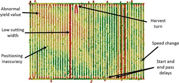
Figure 4 shows one realisation of the simulation process. The colour gradient ranges from bright (low yield values) to dark (high yield values). This simulated dataset exhibits a clear spatial correlation, with low-yielding areas at the centre and North-West of the field and relatively high-yielding areas in the remaining zones. Well-known sources of errors are clearly visible, especially passes harvested with a low cutting width, harvest turns, speed changes, and start and end-pass delays at each start and end rows. This plot shows a relatively high number of transects harvested with a low cutting width, especially in the eastern part of the field. It is acknowledged that these simulated datasets have their limits. For instance, harvest patterns are relatively simple within the fields, i.e. most passes have been considered harvested in straight lines. Only known sources of errors can be modelled which means that some specific cases might not be taken into account during simulations.
An example of synthetic yield dataset. Yield data range from low (bright) to high (dark) values. Corresponding colours are red (low yield values) and green (high yield values) for the coloured image. Be aware that the coloured image is more readable.

Reliability of simulated datasets
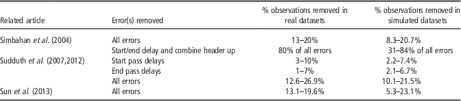
The proportion of defective observations identified by previously reported data filtering methods in simulated datasets was close to that in real datasets (Table 2). The stronger divergence was observed for the approach of Simbahan et al. (Reference Simbahan, Dobermann and Ping2004) according to the proportion of observations acquired during start/end pass delays and those recorded when the combine header was up. Note however that in the simulation process, the combine header was considered down all the time which is why the proportion of observations removed was lower in the simulated datasets in that specific case. It should be noted that the proportion of observations corresponding to start and end pass delays reported by Sudduth et al. (Reference Sudduth and Drummond2007) was only between 42 and 55% of the total number of observations removed, i.e. in the range observed with simulated datasets. The methodologies described by Sudduth et al. (2007, Reference Sudduth, Drummond, Myers and Anatole2012) and Sun et al., (Reference Sun, Whelan, McBratney and Minasny2013) worked similarly between real and simulated datasets.
Output of data filtering methods on real and simulated datasets

Case study: Objective evaluation of a yield filtering approach
The approach of Simbahan et al. (Reference Simbahan, Dobermann and Ping2004) can be evaluated at the whole dataset level and for each known sources of errors (Table 3). Specificity is not detailed for each given type of error because this metric only makes sense for the overall dataset. First of all, the simulation process covers a wide range of cases with varying proportions of outliers of different types. A very detailed evaluation of the approach of Simbahan et al. (Reference Simbahan, Dobermann and Ping2004) is beyond the scope of this work but general conclusions can be reported. Global sensitivity reaches more than 60% which means that a high number of defective observations has been removed. Note that very few normal observations have been filtered out (specificity is above 95%). Be aware that all the observed sensitivity values are not absolute values and should be compared to the outputs of other filtering methods. It is clear that this approach did not identify all types of errors equally. Start and end pass delays are almost detected in all cases because Simbahan et al. (Reference Simbahan, Dobermann and Ping2004) propose to manually select a threshold after looking at the grain flow dynamics along passes. Positioning inaccuracy has a low sensitivity given the fact that Simbahan et al. (Reference Simbahan, Dobermann and Ping2004) do not account for this issue. Other filters, especially that of local outliers, might have detected some of these positioning inaccuracies that most likely had an abnormal yield value with regard to their neighbourhood. The remaining sources of errors, i.e. speed changes, low cutting width or harvest turns among others are assumed to be detected by global and local filters. The ability to detect these errors depends on the outlier distance. For instance, if speed changes are slight, the local outlier filter may miss this. Future analysis could focus on the non-detected outliers to evaluate their influence on the global or local statistics of the dataset.
Sensitivity and specificity (percentage) of the approach proposed by Simbahan et al. (Reference Simbahan, Dobermann and Ping2004) with regard to the detection of known sources of errors. Mean and (standard deviation) of the twenty simulations are reported

Conclusion
A methodology has been proposed to evaluate and compare, objectively and quantitatively, yield filtering methods with regard to their ability to remove defective observations from yield datasets. The proposed simulated datasets might be used to determine to what extent a given approach is robust to a specific type of error or more generally to defective observations. Simulations could also help analyse whether each step of sequential filtering procedures identify only one type of error or a mix of them. Simulated yield datasets can be significantly improved by incorporating more sources of errors, such as, lag time delays, moisture errors, fields harvested by two combines at the same time or harvested in two times, grouped GPS positioning errors, or creating fields with more complex shapes. These simulations do not exempt any filtering approach to be tested on real yield datasets but provide an opportunity for filtering algorithms to be compared and improved.