


1. Introduction
The improvement of the efficiency of marine transportation is a critical target, due to its significant economic and environmental impact (Huang & Duan Reference Huang and Duan2023; Lau et al. Reference Lau, Chen, Poo, Ng and Ying2024; Mollaoglu et al. Reference Mollaoglu, Yazar, Ilknur, Gurturk and Doganer Duman2024; Triantoro et al. Reference Triantoro, Mangan and Rietig2026). A more efficient propulsion means lower fuel consumption with reduced emissions of pollutants and greenhouse gasses into the atmosphere. An option for the achievement of this goal is represented by energy saving device (ESDs), which may be implemented in new installations or retrofitted to existing propulsion systems. A particular class of ESDs are the propeller boss cap fins (PBCFs), which are fins installed downstream of marine propellers, having the purpose of mitigating the intensity of the hub vortex that typically characterises their wake axis. The hub vortex is the largest flow structure shed by axial-flow propellers. It is a wide region of low pressure, generating an unwanted drag, diminishing the overall thrust produced by the propulsion system. PBCFs are therefore able to improve the efficiency of propulsion by reducing the intensity of the hub vortex. Actually, additional benefits to the efficiency of propulsion come from the production of a blockage effect, increasing the pressure levels on the pressure side of the propeller blades. PBCFs also generate a torque opposite to that required for the rotation of the propeller blades, which is also useful to enhance efficiency. Actually, it should be noted that the PBCFs produce a negative thrust (that is, a drag), but the above-mentioned effects usually overcome this drawback. Therefore, these devices are able to improve the efficiency of propulsion by increasing the thrust produced by the overall system and decreasing the torque required for its rotation. Furthermore, the mitigation of the intensity of the hub vortex is possibly beneficial for additional reasons. For instance, the negative peak of pressure produced at the core of the hub vortex is a potential region of cavitation, having a negative impact on the acoustic signature and, in turn, on the environment. This is also critical for the tactical capabilities of military vehicles. Furthermore, marine propellers operate usually upstream of rudders for manoeuvring (Felli & Falchi Reference Felli and Falchi2011). The interaction of the hub vortex with them is especially problematic, causing structural damage, lower performance, and additional vibrations and noise (Paik et al. Reference Paik, Kim, Kim, Kim and Suh2012; Zhang et al. Reference Zhang, Hong, Yang, Jiao and Wang2019; Zhang et al. Reference Zhang, Li, Ma, Ning, Sun and Hu2022). Of course, these issues are substantially reinforced in the case where the fluid within the hub vortex is cavitating.
The literature on the wake system of marine propellers demonstrated the complexity of its flow physics, characterised by multiple flow structures, especially the tip and hub vortices (Felli et al. Reference Felli, Camussi and Di Felice2011; Baek et al. Reference Baek, Yoon, Jung, Kim and Paik2015; Wang et al. Reference Wang, Wu, Gong and Yang2021). They undergo instability phenomena, leading to mutual inductance events, leapfrogging and eventually to break-up into smaller turbulent scales, feeding the process of turbulent energy cascade. Often, the instability process of the hub vortex is slower than that of the tip vortices, making its analysis even more challenging to both experimental and numerical methods, because of its development across distances further downstream of the propeller. In particular, the existing literature demonstrated the limitations of conventional, time-averaged approaches, like Reynolds-averaged Navier–Stokes (RANS) simulations, to reproduce properly the flow physics of the wake (Muscari et al. Reference Muscari, Di Mascio and Verzicco2013; Cai et al. Reference Cai, Li and Liu2019; Sezen et al. Reference Sezen, Atlar and Fitzsimmons2021). RANS was actually found suitable to capture properly the hydrodynamic performance of marine propellers. However, the simulation of the wake flow requires more accurate techniques, such as detached eddy simulation (DES) and LES, on very fine grids, able to resolve a wide range of turbulent scales across the whole process of wake instability (Balaras et al. Reference Balaras, Schroeder and Posa2015; Kumar & Mahesh Reference Kumar and Mahesh2017; Posa et al. Reference Posa, Broglia, Felli, Falchi and Balaras2019; Wang et al. Reference Wang, Liu, Wang and Li2022; Posa Reference Posa2023).
To date, most works in the literature on propellers equipped with PBCFs are focused on the prediction of their impact on the hydrodynamic performance (Kawamura et al. Reference Kawamura, Ouchi and Nojiri2012). Many of them are parametric (Xiong et al. Reference Xiong, Wang and Qi2013; Lim et al. Reference Lim, Kim, Lee, Kang and Kim2014; Tan et al. Reference Tan, Ding, Liu and Sui2023; Tian et al. Reference Tian, Zhao, Ma, Lv, Kang, Wang, Pan, Lin, Ren and Wang2025) or optimisation (Ma et al. Reference Ma, Cai, Qian and Chen2014; Mizzi et al. Reference Mizzi, Demirel, Banks, Turan, Kaklis and Atlar2017; Gaggero Reference Gaggero2018; Gaggero & Martinelli Reference Gaggero and Martinelli2021; Yin et al. Reference Yin, Rosenvinge, Sandland, Ehlers and Shin2023; Li et al. Reference Li, Cao, Xu, Jiang and Liu2024) studies on the efficiency of propulsion, where, typically, RANS is carried out on computational grids consisting of a few million cells. Data from RANS computations were also used by Liu et al. (Reference Liu, Yu, Yu, Yan and He2024) to develop a surrogate model for the prediction of the hydrodynamic and hydroacoustic performance of PBCFs. In the work by Sun et al. (Reference Sun, Su, Wang and Hu2016) the same methodology was adopted to study the interaction between the wake of a propeller with and without PBCFs with downstream straight and twisted rudders. However, the focus was still on the hydrodynamic performance of the propulsion system, rather than on the benefits for the rudders of operating within a weaker hub vortex and the relevant fluid dynamics. As already discussed, RANS is indeed suitable when the interest is towards the thrust generated by the propulsion system and the torque required for its rotation. The above-mentioned works agree on the beneficial effect on the efficiency of propulsion granted by the implementation of PBCFs, which was found to be improved by up to
 $5\,\%$
. Meanwhile, little information is reported on the flow physics and its changes, tied to the mitigation of the intensity of the hub vortex. More details are instead given in the works by Gaggero & Martinelli (Reference Gaggero and Martinelli2021) and Zheng et al. (Reference Zheng, Huang, Zhou, Li, He and Li2024), where DES was adopted.
The main target of the work by Gaggero & Martinelli (Reference Gaggero and Martinelli2021) was actually the implementation of a simulation based design optimisation (SBDO) technique for the development of the geometry of PBCFs to be retrofitted to the Japan bulk carrier (JBC) propeller. In the framework of this process, they used RANS computations. However, this optimal design was then verified by DES computations on a mesh consisting of approximately 32 million cells. They found that PBCFs were indeed very effective in reducing the intensity of the hub vortex shed by the JBC propeller, although the analysis was limited to the first-order statistics of the solution (pressure and velocity fields), with no discussion on the statistics of turbulence. Meanwhile, the presence of the PBCFs was found to move the pairing process of the tip vortices shed by the main rotor of the propeller slightly upstream. However, despite the substantial changes affecting the wake flow, the fluctuations in time of the pressure field were found to be minimally changed, suggesting a limited effect on the acoustic signature of the system. In the same study, unconventional ducted PBCFs were also developed, but the additional nozzle of the PBCFs was not able to produce significant benefits. Actually, the overall performance of the propulsion system was even slightly reduced, compared with that of the conventional PBCFs without a nozzle.
DES was also employed by Zheng et al. (Reference Zheng, Huang, Zhou, Li, He and Li2024) to study the impact of PBCFs on the hydrodynamics and hydroacoustics of a pump jet propeller. These are unconventional propulsion devices equipped with both rotor and stator blades operating within a nozzle. The analysis of the hydroacoustics was carried out by using the Ffowcs Williams & Hawkings (FWH) acoustic analogy (Ffowcs Williams & Hawkings Reference Ffowcs Williams and Hawkings1969). Results were reported from computations conducted on a grid consisting of approximately 25 million cells. Both stationary and rotating PBCFs were considered. The complexity of the wake system was found to be increased by the stationary PBCFs, characterised by the onset of multiple flow structures, due to their unsteady interaction with the flow coming from the main rotor of the propeller. In contrast, the rotating PBCFs were actually useful to diminish the intensity of the hub vortex and to improve the uniformity of the flow at the wake core. However, the analysis of flow physics was limited to the instantaneous realisations of the solution. The overall sound pressure levels were also increased by the stationary PBCFs, while they were not substantially modified by the rotating PBCFs, in comparison with the original propeller.
The influence of contra-rotating PBCFs on the flow physics was analysed by LES in a work by Zhu et al. (Reference Zhu, Zhou, Shu and Hu2022), which adopted computational meshes of up to 55 million cells. Contra-rotating fins are expected to improve the ability of recovering the azimuthal momentum in the wake of the main rotor of the propulsion system, with additional benefits to performance. An improvement in efficiency of propulsion of
 $3\,\%$
was reported. In addition, they found the PBCFs are able to suppress the cavitation phenomena occurring at the axis of the wake of the original propeller. From instantaneous visualisations of the solution, Zhu et al. (Reference Zhu, Zhou, Shu and Hu2022) also identified the signature of a number of smaller vortices within the wake core, replacing the large hub vortex shed by the original propeller.
Yu et al. (Reference Yu, Zhou, Yi, Zou, Han and Luo2025) used a RANS approach for the optimisation of the performance of PBCFs, while LES on a computational grid of 24 million cells was employed for the analysis of the wake instability process. While they verified a dramatic reduction of the negative peak of pressure at the wake axis, thanks to the suppression of the hub vortex, the effect on the tip vortices and their instability process was found to be practically negligible. Zhu & Li (Reference Zhu and Li2025) also adopted an LES methodology on a grid consisting of 16 million cells to explore the influence of geometric parameters of contra-rotating PBCFs on the overall performance. This study included the effects of the diameter, pitch and chord length ratios on the hydrodynamic performance. Unfortunately, little discussion about the influence on the flow physics was reported.
The presented survey demonstrates the limitations of the current literature on the fluid dynamics induced by the implementation of PBCFs. While their benefits in terms of efficiency of propulsion are clear, with several studies also proposing strategies for their optimisation, the impact on the flow physics of the wake is not. For instance, while it is evident that the mitigation of the intensity of the hub vortex brings important advantages in terms of wake signature, the influence of the additional flow structures shed by the PBCFs has not been studied in detail. Is the onset of these structures able to negatively balance the benefit of reducing the intensity of the hub vortex or is their signature relatively small? In other words, while it is clear that PBCFs are able to mitigate the intensity of the hub vortex, the impact of the instability process of the wake system and turbulent stresses by the trailing wake of the PBCFs and the relevant tip vortices was not discussed in detail. This is also the case for the interaction of the root vortices shed by the main rotor with the PBCFs. For instance, is the beneficial effect of the PBCFs originating mainly from their ability to hinder the mutual interaction between the root vortices shed by the main rotor or from a reduction of the azimuthal momentum of the wake at the innermost radii? Furthermore, the impact of these changes on the stability of the outer region of the propeller wake, especially the tip vortices, is not obvious, since the current studies do not agree on this point. Even in the few works where eddy-resolving methodologies were adopted, only first-order statistics and instantaneous visualisations of the solution were reported, with little discussion on the turbulent stresses. Meanwhile, it is important to understand if the increased complexity of the wake topology, due to the trailing wake of the PBCFs, is a source of turbulent stresses of the same order as those attributable to the hub vortex shed by the original propulsion system operating without PBCFs. In addition, it is well known that the accuracy of DES and LES relies on their ability of resolving a wide range of turbulent scales, limiting subgrid scale (SGS) modelling to the smallest, isotropic, most universal ones. Therefore, high levels of resolution should be granted not only within the region of the propeller and PBCFs, but also downstream of them, across the whole process of instability of the wake structures.
To address the limitations of the current literature on the subject, in the present study, results of high-fidelity LES computations on a grid consisting of almost 7 billion points are reported, dealing with the five-bladed JBC propeller, equipped with PBCFs. Their geometry was developed in the framework of the earlier optimisation study by Gaggero & Martinelli (Reference Gaggero and Martinelli2021). This work is focused on the analysis of the wake flow, and the comparison between the cases with and without PBCFs to clarify their influence on the intensity of the flow structures, their interaction, their process of instability, and the statistics of turbulence across three working conditions. In particular, this study shows that, while the hub vortex experiences a dramatic mitigation, the additional vortices shed by the PBCFs are substantially less intense, resulting eventually also in lower turbulent stresses. In addition, the flow structures populating the wake core, shed by both the main rotor and the PBCFs, are more stable than those of the original propulsion system. These changes are attributable to the smaller shear with a less intense hub vortex, and the larger pitch of the helical vortices from both the main rotor and the PBCFs, due to the reduction of the azimuthal momentum at the wake core. Therefore, the impact of the PBCFs in terms of attenuation of pressure minima and turbulence maxima within the wake core is indeed very significant, with potential benefits on cavitation and radiated sound. Moreover, while the earlier studies in the literature were found to disagree on the effect of PBCFs on the process of instability of the tip vortices, the present computations reveal little influence on the flow structures at the outer boundary of the propeller wake, despite the dramatic changes affecting its core.
In the following, the present study is structured in the discussion of the methodology (§ 2), the particular flow problem (§ 3), the computational set-up (§ 4), the analysis of the results (§ 5) and the conclusions (§ 6).
2. Methodology
The present flow problem is governed by the Navier–Stokes equations for incompressible flows. They were resolved in non-dimensional form:
 \begin{eqnarray} {\partial \widetilde {u}_i \over \partial x_i} = 0, \;\;\; i=1,2,3, \\[-28pt] \nonumber \end{eqnarray}
 \begin{eqnarray} {\partial \widetilde {u}_i \over \partial t} + {\partial \widetilde {u}_i \widetilde {u}_{\kern-1pt j} \over \partial x_{\kern-1pt j} } = - {\partial \tilde {p} \over \partial x_i} - {\partial \tau _{\textit{ij}} \over \partial x_{\kern-1pt j}} + {1 \over \textit{Re}} {\partial ^2 \widetilde {u}_i \over \partial x_{\kern-1pt j}^2} + f_i, \;\;\;i,j=1,2,3, \\[0pt] \nonumber \end{eqnarray}
where (2.1) and (2.2) represent the conservation of mass and momentum, respectively. In those equations,
 $x_i$
is the coordinate in the direction
 $i$
in space,
 $t$
is time,
 $\widetilde {u}_i$
is the filtered velocity and
 $\tilde {p}$
is the filtered pressure. Additionally,
 $\textit{Re}=\rho V L/\mu = V L/\nu$
is the Reynolds number, which is the result of scaling the dimensional equations by using a reference velocity scale,
 $V$
, a reference length scale,
 $L$
, and the density of the fluid,
 $\rho$
, while
 $\mu$
and
 $\nu$
are the dynamic and kinematic viscosities of the fluid, respectively.
The quantity
 $\tau _{\textit{ij}}=\widetilde {u_i u_{\kern-1pt j}} - \widetilde {u}_i \widetilde {u}_{\kern-1pt j}$
is the SGS stress tensor, which results from filtering the Navier–Stokes equations. They are indeed discretised on a computational grid that is, in general, not able to resolve all turbulent scales of the flow. The size of the filter,
 $\varDelta$
, is practically defined by the local resolution of the computational grid. The SGS stress tensor is required to take into account the action of the smallest scales of the flow, which are smaller than the spacing of the computational grid, on the largest, resolved scales. Therefore, the problem of turbulence closure consists in properly modelling
 $\tau _{\textit{ij}}$
. This is achieved by using an eddy-viscosity hypothesis, which assumes that the deviatoric part of the SGS tensor is aligned with the deformation tensor of the resolved velocity field,
 $\widetilde {\mathcal{S}}_{\textit{ij}}$
:
 \begin{align} \tau _{\textit{ij}}^d = \tau _{\textit{ij}} - {1 \over 3} \delta _{\textit{ij}} \tau _{kk} = -2 \nu _t \widetilde {\mathcal{S}}_{\textit{ij}}, \;\;\;i,j=1,2,3, \end{align}
where
 $\delta _{\textit{ij}}$
is the Kronecker delta,
 $\tau _{kk}$
is the trace of the SGS tensor and
 $\nu _t$
is the eddy-viscosity. This hypothesis reduces the problem of turbulence closure from modelling the six independent elements of the symmetric tensor
 $\tau _{\textit{ij}}$
to the only scalar eddy-viscosity. In this study, this problem was resolved by using the wall-adaptive local eddy-viscosity (WALE) model by Nicoud & Ducros (Reference Nicoud and Ducros1999), representing
 $\nu _t$
by means of the deviatoric part of the square of the velocity gradient tensor of the resolved field,
 $\widetilde {\mathcal{G}}_{\textit{ij}}^d$
:
 \begin{align} \nu _t= (K \Delta )^2 {\left ( \widetilde {\mathcal{G}}_{\textit{ij}}^d \widetilde {\mathcal{G}}_{\textit{ij}}^d \right )^{3/2} \over \left ( \widetilde {\mathcal{S}}_{\textit{ij}} \widetilde {\mathcal{S}}_{\textit{ij}} \right )^{5/2} + {\left ( \widetilde {\mathcal{G}}_{\textit{ij}}^d \widetilde {\mathcal{G}}_{\textit{ij}}^d \right )^{5/4}}}, \;\;\;i,j=1,2,3, \end{align}
where
 $K=0.5$
is a constant, while
 $\Delta$
is the size of the filter, which is practically the local size of the computational grid, computed as the cube root of each grid cell. This particular representation of the eddy-viscosity features several convenient properties. For instance, it takes into account both deformation and rotation of the resolved velocity field. This way, it is able to switch off in regions of laminar gradients with no turbulence. In addition, the expression in (2.4) was properly designed to reproduce the correct limiting behaviour of
 $\nu _t$
in the vicinity of solid walls, scaling as the cube of the distance from them. Moreover, in our experience, this is a quite inexpensive model, resulting in an overhead equivalent to only a few percent of the overall computational cost, making it suitable to handle computationally demanding problems, such as that in the present study.
The last quantity in (2.2) is a forcing term, which was used to represent the action of the bodies within the flow by means of an immersed boundary (IB) methodology. This relaxes the requirement for the Eulerian grid, discretising the computational domain where the governing equations are resolved, to fit the geometry of the bodies immersed within the flow. These are represented by suitable Lagrangian grids, discretising their surface and ‘immersed’ within the Eulerian grid, free to move across its cells without deformation or regeneration of the Eulerian grid. Based on their position relative to the Lagrangian grids, the Eulerian points are identified as ‘solid’, ‘fluid’ or ‘interface’. In the present implementation of the IB methodology (Balaras Reference Balaras2004; Yang & Balaras Reference Yang and Balaras2006), the interface points are those placed outside the region encompassed by the Lagrangian grid, but having, across any coordinate direction, at least a neighbouring solid point, which is an Eulerian point within that region. All other points outside the immersed boundaries are tagged as fluid. Boundary conditions are required at the interface and solid points. At the solid points, the boundary condition,
 $\mathcal{U}_i$
, is the velocity of the body where the particular Eulerian point is placed. At the interface points, the velocity condition,
 $\mathcal{U}_i$
, comes from a local reconstruction of the solution along the direction normal to the surface of the Lagrangian grid. This is a trilinear interpolation using the no-slip requirement on the surface of the Lagrangian grid and the solution at the fluid points surrounding the particular interface point as boundary conditions. Therefore, the forcing term,
 $f_i$
, is computed as
 \begin{align} f_i = {\mathcal{U}_i - \widetilde {u}_i \over \Delta t} - \mathcal{R}_i, \;\;\; i=1,2,3, \end{align}
where
 $\Delta t$
is the step of the advancement in time of the numerical solution,
 $\widetilde {u}_i$
is the velocity along the direction
 $i$
in space at the particular interface or solid point from the last time level, while
 $\mathcal{R}_i$
is the sum of all convective, viscous, SGS and pressure gradient terms of (2.2), all computed explicitly for the definition of the IB conditions.
The governing equations were discretised in space by using second-order, central-differences on a staggered grid in cylindrical coordinates. The hepta-diagonal Poisson problem stemming from the continuity requirement of (2.1) was decomposed into a series of penta-diagonal problems by using trigonometric transformations along the azimuthal direction. Then, each penta-diagonal system of equations was inverted by means of an efficient direct solver (Rossi & Toivanen Reference Rossi and Toivanen1999). The advancement in time was carried out by using a fractional-step methodology (Van Kan Reference Van Kan1986). All terms of radial and axial derivatives of the momentum equation were discretised explicitly in time by means of the three-step Runge–Kutta scheme. For all terms of azimuthal derivatives, the implicit Crank–Nicolson scheme was adopted, to relax the stability requirements arising at the axis of the cylindrical grid.
The overall Navier–Stokes solver, including its IB implementation, was validated on several canonical flow problems, demonstrating its second-order accuracy in both space and time (Balaras Reference Balaras2004; Yang & Balaras Reference Yang and Balaras2006; Yang et al. Reference Yang, Preidikman and Balaras2008). It was also used in several cases involving marine propellers, including also validations against physical experiments (Posa et al. Reference Posa, Broglia, Felli, Falchi and Balaras2019, Reference Posa, Broglia and Balaras2022, Reference Posa, Capone, Alves Pereira, Di Felice and Broglia2024, Reference Posa2025, Posa Reference Posa2025). Note that, in this section, all filtered variables were indicated as
 $\widetilde {\varphi }$
, where
 $\varphi$
represents any physical quantity. However, since in the following discussion only resolved fields will be discussed, for convenience that notation will be omitted hereafter.
Geometries of the (a)
 $ \textit{REF}$
and (b)
 $ \textit{MOD}$
cases.

3. Flow problem
In this study, the JBC five-bladed propeller is considered (Larsson et al. Reference Larsson, Stern, Visonneau, Hirata, Hino and Kim2015). This was simulated without and with five PBCFs, which are the result of an earlier work (Gaggero & Martinelli Reference Gaggero and Martinelli2021), aimed at the optimisation of the hydrodynamic performance of the propulsion system. The PBCFs move together with the main rotor of the propeller. The two geometries without and with PBCFs will be indicated herein as
 $\textit{REF}$
and
 $\textit{MOD}$
, respectively. They are illustrated in figure 1. Simulations were carried out in open-water conditions, which means that the propeller inflow is axial and uniform.
The working conditions of marine propellers are characterised through the advance coefficient and the Reynolds number, defined as
 \begin{align} J = {V \over nD}, \;\;\;\;\;\; Re_{70\,\%R} = {c_{70\,\%R}\sqrt {(2 \pi n \; 0.7R)^2+V^2} \over \nu _w}, \end{align}
where
 $J$
is the advance coefficient;
 $V$
the advance velocity;
 $n$
the frequency of the rotation of the propeller;
 $D$
its diameter;
 $Re_{70\,\%R}$
the Reynolds number, referred to
 $70\,\%$
of the radial extent of the propeller,
 $R$
;
 $c_{70\,\%R}$
the chord of the propeller blades at the same radial location; while
 $\nu _w$
is the kinematic viscosity of water.
Three values of the advance coefficient were simulated,
 $J=0.300$
,
 $0.456$
and
 $0.600$
. Here,
 $J=0.456$
is the advance coefficient of design of the JBC propeller, which is also the working condition for which the geometry of the PBCFs was optimised. The other values of
 $J$
were simulated to verify the ability of the PBCFs of mitigating the intensity of the hub vortex even at higher and lower loads, respectively, away from the design. All computations were conducted with a value of
 $Re_{70\,\%R} \approx 400\,000$
. For validation, physical experiments (Larsson et al. Reference Larsson, Stern, Visonneau, Hirata, Hino and Kim2015) as well as RANS computations are available at the same working conditions.
4. Computational set-up
LES was carried out within a cylindrical domain having a radial extent equal to
 $5.0D$
and ranging from
 $2.5D$
upstream of the propeller up to
 $7.5D$
downstream. Note that the origin of the streamwise coordinates was placed at the boundary between the upstream stationary shaft and the hub of the rotor of the JBC propeller. A uniform axial velocity was enforced at the inlet of the domain to reproduce open-water conditions. Convective conditions were imposed at the outflow boundary. Neumann conditions with impermeability at the lateral, cylindrical boundary were used to mimic a free stream. Zero-gradient conditions were also enforced for pressure and eddy-viscosity at all external boundaries of the domain. On the surface of the bodies immersed within the flow, the no-slip requirement was imposed by using the IB methodology discussed in § 2.
The domain was discretised by using a cylindrical grid consisting of
 $714 \times 3074 \times 3074$
(6.75 billion) points along the radial, azimuthal and streamwise directions, respectively. The angular spacing of the azimuthal grid,
 $\Delta \vartheta$
, was uniform, resulting in an increasing resolution (decreasing linear azimuthal spacing,
 $r \Delta \vartheta$
) towards inner radial coordinates, characterised by the highest gradients of the solution. The radial and axial grids were refined in the region of the propeller and its wake. The radial grid was uniform in the region
 $r/D \lt 0.6$
, encompassing the whole propeller and its wake system. It was stretched farther away up to the lateral boundary of the domain to save grid points. The axial grid was also uniform across the region of the propeller blades and the PBCFs,
 $0.0 \lt z/D \lt 0.35$
, and was stretched both upstream and downstream. However, the downstream stretching was kept smooth up to
 $z/D=6.0$
to resolve accurately the wake flow. More details about the radial and axial distributions of the grid spacing are reported in figure 2, while a meridian slice is represented in figure 3, where only a small sample of points is shown, for visibility of the grid lines. The average resolution of the Eulerian grid was verified to be equivalent to approximately 5 wall-units. For example, figure 4 represents the resolution of the Eulerian grid in wall-units on the surface of the blades of the main rotor and the PBCFs, based on the computations carried out for the
 $ \textit{MOD}$
case at the design working condition. Note that the same Eulerian grid was adopted to simulate both
 $ \textit{REF}$
and
 $ \textit{MOD}$
, for the accuracy of the comparison between the two cases. To verify grid-independence, the design working condition,
 $J=0.456$
, was also simulated on coarser grids for both
 $ \textit{REF}$
and
 $ \textit{MOD}$
. They were generated by reducing the number of points along each direction in space by factors equal to
 $\sqrt [3]{2}$
and
 $\sqrt [3]{4}$
, resulting in an overall reduction equal to
 $2$
and
 $4$
on the ‘medium’ and ‘coarse’ grids, relative to the ‘fine’ grid discussed earlier. Therefore, the medium and coarse grids consisted of
 $566 \times 2442 \times 2442$
(3.38 billion) and
 $450 \times 1938 \times 1938$
(1.69 billion) points, respectively. In the following discussion, results will be reported on the fine grid, unless otherwise stated. The geometries immersed within the flow were represented by Lagrangian grids. They consisted of an overall number of elements (triangles) equal to approximately
 $180\,000$
and
 $315\,000$
for the
 $ \textit{REF}$
and
 $ \textit{MOD}$
cases, respectively. These Lagrangian grids are represented in figure 5.
(a) Radial and (b) axial spacings of the fine Eulerian grid.

Visualisations of a meridian slice of the fine Eulerian grid: (a) global and (b) detailed views. For visibility of the grid lines, only one of every 256 and 64 points shown in panels (a) and (b), respectively.

Resolution of the computational grid in wall-units: (a,b) suction and pressure sides of the blades of the main rotor of the propeller; (c,d) pressure and suction sides of the PBCFs. Visualisations from the simulation of the
 $ \textit{MOD}$
case at the design working condition.

(a) Upstream and (b) downstream views of the Lagrangian grids.

Due to stability requirements, the resolution in time was very fine. The non-dimensional time step was equal to
 $\Delta t U/D = 0.65 \times 10^{-4}$
. For the three increasing advance coefficients, this value resulted in approximately
 $4600$
,
 $7000$
and
 $9200$
time steps for a full revolution. All simulations were advanced in time for two flow-through times to develop statistically steady conditions in the wake. Then, both time-averaged and phase-averaged statistics were computed at run time during 10 additional revolutions. The former were computed in a stationary reference frame, while the latter in a reference frame rotating together with the propeller. They will be indicated as
 $\overline {\mathcal{\varphi }}$
and
 $\widehat {\mathcal{\varphi }}$
, respectively. The fluctuations in time will be represented as
 $\varphi '$
and the relevant time-averaged and phase-averaged mean squares as
 $\overline {\varphi '\varphi '}$
and
 $\widehat {\varphi '\varphi '}$
, respectively. In particular, the time-averaged and phase-averaged turbulent kinetic energies are defined as
 \begin{align} \overline {k} = {1 \over 2} \big (\overline {u'u'} + \overline {v'v'} + \overline {w'w'} \big ), \quad \widehat {k} = {1 \over 2} \big (\widehat {u'u'} + \widehat {v'v'} + \widehat {w'w'} \big ), \end{align}
where
 $u$
,
 $v$
and
 $w$
are the radial, azimuthal and streamwise velocity components, respectively.
All simulations were performed through high-performance computing by using an in-house-developed Fortran solver with MPI (message passing interface) capabilities, enabling parallel computations. All cylindrical problems were decomposed along the streamwise direction in cylindrical subdomains. In particular, the computations on the fine, medium and coarse grids were distributed across
 $768$
,
 $610$
and
 $484$
cores of a pre-exascale supercomputer (Leonardo DCGP, CINECA, Italy). The overall computational cost of the simulations was equivalent to approximately 16 million core hours.
5. Results
5.1. Global performance and grid uncertainty
In this section, results for the global performance are reported, including also comparisons with experiments available in the literature (Larsson et al. Reference Larsson, Stern, Visonneau, Hirata, Hino and Kim2015) and RANS computations. The relevant parameters are defined as
 \begin{align} K_T = {T \over \rho n^2 D^4},\;\;\; K_Q = {Q \over \rho n^2 D^5}, \;\;\; \eta = {J K_T \over 2\pi K_Q}, \end{align}
where
 $T$
is the thrust produced by the propulsion system and
 $Q$
is the torque required for its rotation. The coefficient
 $\eta$
represents how well the torque required for the rotation of the propeller is used to generate thrust.
Table 1 reports the time-averaged values of the parameters of performance from the present LES computations on the JBC propeller without PBCFs as well as from experiments (EXP) in the literature and the RANS computations conducted to compare with LES. It is useful to recall that, although the limitations of RANS for the analysis of the wake flow are well known, it is considered accurate enough for the computation of the loads acting on marine propellers in open-water conditions (Li Reference Li2006; Dong et al. Reference Dong, Li, Yang and Noblesse2018; Nouroozi & Zeraatgar Reference Nouroozi and Zeraatgar2019). RANS was carried out using the Shear Stress Transport
 $\kappa {-}\omega$
turbulence model on grids consisting of 5.5 and 7.5 million hexahedral cells, discretising a single vane of the
 $ \textit{REF}$
and
 $ \textit{MOD}$
geometries, respectively. The deviations of LES from the experiments and RANS are indicated as
 $e_{\textit{EXP}}$
and
 $e_{\textit{RANS}}$
, respectively. The agreement with the experiments is good and better than that with the RANS computations. Although errors keep within a few percent, RANS systematically estimates lower values of thrust and higher values of torque in comparison with LES and the experiments, resulting in lower levels of efficiency of propulsion. The following discussion will show that this is the case also for the modified geometry of the propulsion system, including PBCFs.
Time-averaged parameters of performance of the
 $ \textit{REF}$
propeller: comparison of the LES computations on the fine grid with experiments in the literature (Larsson et al. Reference Larsson, Stern, Visonneau, Hirata, Hino and Kim2015) and RANS computations.

Table 1. Long description
The table compares time-averaged parameters of performance of the REF case using LES computations, experiments, and RANS computations. It has 5 rows and 9 columns. The columns are labeled with different parameters and their values at three different J values: 0.300, 0.456, and 0.600. The rows are labeled as LES, EXP, e_EXP, RANS, and e_RANS. Each row contains values for K_T, 10*K_Q, and η at the specified J values. The table also includes deviations of LES from experiments and RANS, indicated as e_EXP and e_RANS, respectively.
Time-averaged parameters of performance of the
 $ \textit{MOD}$
propeller: comparison of the LES computations on the fine grid with RANS computations and with the LES computations on the
 $ \textit{REF}$
propeller.

Table 2. Long description
A table comparing propeller performance parameters for the MOD case using LES and RANS computations. The table has 5 rows and 9 columns. Column headers are K_T, 10K_Q, and η for three different values of J (0.300, 0.456, 0.600). Row labels are LES, RANS, e_RANS, Δ_PBCF, and δ_PBCF. Row 1: LES, 0.2645, 0.3111, 40.59 percent, 0.1996, 0.2555, 56.70 percent, 0.1361, 0.1952, 66.56 percent. Row 2: RANS, 0.2540, 0.3148, 38.53 percent, 0.1933, 0.2625, 53.45 percent, 0.1324, 0.2031, 62.25 percent. Row 3: e_RANS, +4.13 percent, -1.17 percent, +5.37 percent, +3.25 percent, -2.66 percent, +6.08 percent, +2.78 percent, -3.87 percent, +6.92 percent. Row 4: Δ_PBCF, +0.66 percent, -2.46 percent, +3.20 percent, -1.20 percent, -2.00 percent, +0.82 percent, +0.39 percent, -1.97 percent, +2.41 percent. Row 5: δ_PBCF, -0.0080, -0.0097, --, -0.0059, -0.0074, --, -0.0050, -0.0065, --.
Contours of pressure coefficient on the pressure side of the propeller blades of the (a,c,e)
 $ \textit{REF}$
and (b,d,f)
 $ \textit{MOD}$
geometries from phase-averaged statistics: (a,b)
 $J=0.300$
; (c,d)
 $J=0.456$
; (e,f)
 $J=0.600$
.

Figure 6. Long description
The image contains six 3D models of both REF and MOD geometries, each showing the pressure coefficient on the blades. Panel A: A 3D model of the REF propeller with contours of pressure coefficient ranging from -10.0 to 10.0 at the advance coefficient J = 0.300. Panel B: A 3D model of the MOD propeller with contours of pressure coefficient ranging from -10.0 to 10.0 at the advance coefficient J = 0.300. Panel C: A 3D model of the REF propeller with contours of pressure coefficient ranging from -5.0 to 5.0 at the advance coefficient J = 0.456. Panel D: A 3D model of the MOD propeller with contours of pressure coefficient ranging from -5.0 to 5.0 at the advance coefficient J = 0.456. Panel E: A 3D model of the REF propeller with contours of pressure coefficient ranging from -3.0 to 3.0 at the advance coefficient J = 0.600. Panel F: A 3D model of the MOD propeller with contours of pressure coefficient ranging from -3.0 to 3.0 at the advance coefficient J = 0.600. Each panel includes a color bar indicating the pressure coefficient values.
Table 2 provides the results on the global parameters of performance for
 $ \textit{MOD}$
. In this case, no experiments are available and RANS computations were performed for comparison. The deviations of LES from RANS are similar to those found on the original JBC propeller with no PBCFs. In the same table 2, the percentage variation of each parameter from the
 $ \textit{REF}$
propeller is also reported, indicated as
 $\Delta _{\textit{PBCF}}$
and computed from the results of the LES simulations. At all advance coefficients, the efficiency of propulsion experiences an improvement. Despite the negative thrust generated by the PBCFs, this improvement comes from the reduction of the torque required for the rotation of the propulsion system, thanks to the PBCFs producing a torque which is opposite to that acting on the main rotor of the propeller. For better clarity about this point, the last row in table 2 reports as
 $\delta _{\textit{PBCF}}$
the components of thrust and torque coefficients attributable to the PBCFs, again from the LES computations. At
 $J=0.300$
and
 $J=0.600$
, even a slight improvement in the overall thrust generated by the propulsion system occurs. As a result, for these cases, the improvement in efficiency of propulsion is even better than at
 $J=0.456$
. The PBCFs are able to mitigate the strong peak of negative pressure produced at the rear of the propulsion system, due to the onset of the hub vortex. This is very evident from the comparison of the left and right panels of figure 6, where phase-averaged contours of pressure coefficient are shown on the surface of the bodies immersed within the flow. The pressure coefficient was defined as
 \begin{align} c_p = {p-P \over {1 \over 2} \rho U^2}, \end{align}
where
 $P$
is the free stream pressure. In addition, the blockage generated by the PBCFs results in a modified pressure field on the pressure side of the propeller blades, with a slight increase in the values of pressure coefficient at the innermost radii. The overlapping effects of these changes increase both thrust and torque on the main rotor of the JBC propeller. However, this rise is more significant for the former quantity, resulting in an overall improvement in the efficiency of propulsion.
The installation of the PBCFs requires extending the hub, including an additional conical section. This also provides a contribution to the loads, but it is small, if compared with that attributable to the fins. This is reported in table 3, showing that the thrust due to the hub of the PBCFs is only a few percent of their overall thrust. Note that this information is available from the RANS computations only. For the torque coefficient, this contribution is even smaller, since the hub is axisymmetric and its torque is only due to viscous forces. To clarify this point further, additional RANS computations were carried out on the JBC propeller equipped with the hub of the PBCFs, but without including their fins. The relevant results are provided in table 4, showing changes in performance which are an order of magnitude smaller than those reported in table 2. The relative variation in performance, compared with the original geometry, was indicated as
 $\Delta _{\textit{hub}}$
. This change is positive, since the additional conical section of the hub improves the pressure recovery. As a result, the drag due to the rear of the hub is slightly diminished, if compared with the original geometry. These results highlight that the modification of the geometry of the hub, required for the installation of the PBCFs, has little effect on performance, whose improvement is mostly attributable to the fins operating in the wake of the main rotor of the propeller.
Time-averaged parameters of performance of the
 $ \textit{MOD}$
propeller: contribution of the hub of the PBCFs to their overall loads from the data of RANS computations.

Table 3. Long description
A table reporting the contribution of the PBCFs to the overall thrust and torque coefficients. The table has six columns and one row. Column headers are K_T and K_Q for each value of the advance coefficient. Row labels are percentage values. Row 1: 4.11 percent, 0.28 percent, 3.03 percent, 0.36 percent, 10.44 percent, 0.42 percent.
Time-averaged parameters of performance of the
 $ \textit{REF}$
propeller, including the hub of the PBCFs: comparison with the original geometry, based on results from RANS computations.

Table 4. Long description
The table presents a comparison of time-averaged performance parameters of a propeller, including the hub of the PBCFs, against the original geometry based on RANS computations. It has 2 rows and 9 columns. The columns are labeled as K_T, 10K_Q, and η for three different values of J (0.300, 0.456, and 0.600). The rows are labeled as RANS and Δ_hub. Row 1: RANS, 0.2531, 0.3217, 37.57 percent, 0.1932, 0.2672, 52.48 percent, 0.1331, 0.2066, 61.51 percent. Row 2: Δ_hub, plus 0.17 percent, plus 0.03 percent, plus 0.14 percent, plus 0.21 percent, plus 0.10 percent, plus 0.11 percent, plus 0.27 percent, plus 0.13 percent, plus 0.14 percent.
As discussed in § 4, for the advance coefficient
 $J=0.456$
, additional LES computations were carried out also on the medium and coarse Eulerian grids. The relevant results are reported in tables 5 and 6 for the
 $ \textit{REF}$
and
 $ \textit{MOD}$
cases, respectively. In those tables,
 $e_{\textit{fine}}$
represents the deviations of the results dealing with the parameters of performance from the relevant LES computations on the fine grid. The differences across grid resolutions keep within a few percent. As a result, the deviations from the reference experiments and RANS computations also keep of the same order as those found on the fine grid.
Time-averaged parameters of performance of the
 $ \textit{REF}$
propeller: comparison of the LES computations on the medium and coarse grids with experiments in the literature (Larsson et al. Reference Larsson, Stern, Visonneau, Hirata, Hino and Kim2015), RANS computations and the LES computations on the fine grid.

Table 5. Long description
A table comparing propeller performance parameters across different computational methods and grid resolutions for the REF case. The table has 4 rows and 6 columns. Column headers are K_T, 10K_Q, Eta, for both medium and coarse grids. Row labels are LES, e_EXP, e_RANS, and e_fine. Row 1: 0.2000; 0.2594; 55.96 percent; 0.1989; 0.2565; 56.30 percent. Row 2: plus 0.77 percent; minus 2.40 percent; plus 3.33 percent; plus 0.25 percent; minus 3.50 percent; plus 3.96 percent. Row 3: plus 3.71 percent; minus 2.84 percent; plus 6.74 percent; plus 3.17 percent; minus 3.93 percent; plus 7.39 percent. Row 4: minus 1.00 percent; minus 0.50 percent; minus 0.50 percent; minus 1.51 percent; minus 1.62 percent; plus 0.11 percent.
Time-averaged parameters of performance of the
 $ \textit{MOD}$
propeller: comparison of the LES computations on the medium and coarse grids with RANS computations and the LES computations on the fine grid.

Table 6. Long description
The table compares time-averaged parameters of performance for the MOD case across different computational grids and methods. It has 3 rows and 6 columns. The columns are labeled as follows: K_T, 10K_Q, and eta under Medium grid and Coarse grid. The rows are labeled as LES, e_RANS, and e_fine. The values in the table are as follows: Row 1: 0.1981, 0.2560, 56.16 percent, 0.1929, 0.2513, 55.72 percent. Row 2: plus 2.51 percent, minus 2.44 percent, plus 5.07 percent, minus 0.18 percent, minus 4.25 percent, plus 4.25 percent. Row 3: minus 0.72 percent, plus 0.22 percent, minus 0.95 percent, minus 3.33 percent, minus 1.64 percent, minus 1.72 percent.
Additional details on the level of grid dependence of the results for
 $J=0.456$
are reported in table 7. The values of the grid convergence index (GCI), as defined in the work by Celik et al. (Reference Celik, Ghia, Roache, Freitas, Coleman and Raad2008), were computed from time-averaged statistics across the wake of the propeller in a region extending radially in the range of
 $0.0 \lt r/D \lt 0.5$
and axially in the range of
 $0.2 \lt z/D \lt 7.0$
. Then, those values were averaged across all points of the Eulerian grid within this region of the computational domain. Values are reported for both first-order and second-order statistics, for which more details will be provided in the following sections of the manuscript.
Values of the grid convergence index (GCI) (Celik et al. Reference Celik, Ghia, Roache, Freitas, Coleman and Raad2008) computed from time-averaged statistics in the wake region in the ranges of
 $0.0 \lt r/D \lt 0.5$
and
 $0.2 \lt z/D \lt 7.0$
, and averaged across all points of the Eulerian grid.

Table 7. Long description
A table comparing grid convergence index values for different statistical measures. The table has two rows labeled REF and MOD, and eight columns with headers: u_r, u_θ, u_z, c_p, k, u’w’, u’v’, and v’w’. Each column contains percentage values. Row REF: u_r, 9.26 percent; u_θ, 2.35 percent; u_z, 4.04 percent; c_p, 8.09 percent; k, 11.10 percent; u’w’, 12.97 percent; u’v’, 15.96 percent; v’w’, 21.29 percent. Row MOD: u_r, 8.53 percent; u_θ, 16.45 percent; u_z, 0.48 percent; c_p, 6.70 percent; k, 5.11 percent; u’w’, 8.02 percent; u’v’, 8.53 percent; v’w’, 15.64 percent.
Isosurfaces of pressure coefficient from instantaneous realisations of the solution of the (a,c,e)
 $ \textit{REF}$
and (b,d,f)
 $ \textit{MOD}$
geometries, coloured by contours of vorticity magnitude, scaled by
 $U/D$
: (a,b)
 $J=0.300$
(
 $c_p=-5.0$
), (c,d)
 $J=0.456$
(
 $c_p=-1.5$
) and (e,f)
 $J=0.600$
(
 $c_p=-0.3$
). Note that different values were selected for the pressure coefficient and the colour scale of the vorticity magnitude across working conditions.

Figure 7. Long description
Panel A: A 3D plot showing isosurfaces of pressure coefficient for the REF geometry, colored by contours of vorticity magnitude at the advance coefficient J = 0.300. The color scale ranges from 0 to 400. Panel B: A 3D plot showing isosurfaces of pressure coefficient for the MOD geometry, colored by contours of vorticity magnitude at the advance coefficient J = 0.300. The color scale ranges from 0 to 400. Panel C: A 3D plot showing isosurfaces of pressure coefficient for the REF geometry, colored by contours of vorticity magnitude at the advance coefficient J = 0.456. The color scale ranges from 0 to 200. Panel D: A 3D plot showing isosurfaces of pressure coefficient for the MOD geometry, colored by contours of vorticity magnitude at the advance coefficient J = 0.456. The color scale ranges from 0 to 200. Panel E: A 3D plot showing isosurfaces of pressure coefficient for the REF geometry, colored by contours of vorticity magnitude at the advance coefficient J = 0.600. The color scale ranges from 0 to 100. Panel F: A 3D plot showing isosurfaces of pressure coefficient for the MOD geometry, colored by contours of vorticity magnitude at the advance coefficient J = 0.600. The color scale ranges from 0 to 100.
5.2. Flow structures in the wake
The comparison between the instantaneous visualisations in the left and right columns of figure 7 demonstrates that the PBCFs are very effective in mitigating the intensity of the hub vortex. They show isosurfaces of pressure coefficient across the three simulated advance coefficients, and deal with the cases
 $ \textit{REF}$
and
 $ \textit{MOD}$
, respectively. The major flow structures in the wake are locations of intense pressure minima, which are useful to their identification. Note that the intensity of the wake structures and the resulting minima of pressure at their core are a function of the advance coefficient. Therefore, different values of
 $c_p$
were selected across the three working conditions considered in figure 7 to isolate the hub vortex, since the main purpose is the comparison between
 $ \textit{REF}$
and
 $ \textit{MOD}$
for each advance coefficient, for which homogeneous values were adopted for both pressure coefficient and vorticity magnitude. These results show that the PBCFs are able to keep their beneficial effect in mitigating the intensity of the hub vortex also away from design working conditions. This is especially important, also taking into account the long-standing signature of the hub vortex within the wake system, if compared, for instance, with the tip vortices.
Isosurfaces of the second invariant of the velocity gradient tensor from phase-averaged statistics of the solution of the (a,c,e)
 $ \textit{REF}$
and (b,d,f)
 $ \textit{MOD}$
geometries, coloured by contours of vorticity magnitude, scaled by
 $U/D$
: (a,b)
 $J=0.300$
(
 $\widehat {\mathcal{Q}}D^2/U^2=500$
); (c,d)
 $J=0.456$
(
 $\widehat {\mathcal{Q}}D^2/U^2=200$
); (e,f)
 $J=0.600$
(
 $\widehat {\mathcal{Q}}D^2/U^2=50$
). Note that different values were selected for
 $\widehat {\mathcal{Q}}$
and the colour scale of the vorticity magnitude across working conditions.

The
 $\mathcal{Q}$
-criterion (Jeong & Hussain Reference Jeong and Hussain1995) was adopted in figure 8 on phase-averaged statistics. This is able to provide additional details on the wake features. In agreement with earlier studies, the hub vortex is the most stable flow structure (Felli et al. Reference Felli, Camussi and Di Felice2011). The phase-averaged signature of the tip vortices is lost more quickly, since they undergo a faster instability, disrupting their synchronisation with the rotation of the propeller blades. This is also the case of the weaker vortices at the intermediate radii between the tip and hub vortices, populating the trailing wake of the propeller blades. At the advance coefficient of design, the tip vortices in the
 $ \textit{MOD}$
case experience a slightly faster instability, leading to their faster diffusion in the phase-averaged fields, as shown by the comparison between figures 8(c) and 8(d). However, this is only a minor effect, actually missing at the other advance coefficients, for which the deviations between the contours of the tip vortices become practically indistinguishable. Overall, the influence of the PBCFs on the tip vortices is negligible, if compared with the substantial changes affecting the wake axis. In addition to the mitigation of the hub vortex, a reinforced coherence of the helical vortices is visible at the innermost radii for
 $ \textit{MOD}$
, if compared with
 $ \textit{REF}$
. We verified that this change is attributable not only to the additional helical structures shed by the PBCFs, but also to a slower development of instability phenomena for the vortices shed by the main rotor in the range of the radial coordinates of the PBCFs. The reduction of the stresses at the innermost radii, tied to a weaker hub vortex, is able to slow down the instability process of the flow structures populating the core of the propeller wake, if compared with the case without PBCFs. It is also important to recall that the instability process of the helical vortices populating the wake of axial-flow propellers is promoted by mutual inductance events, following the development of short-wave and long-wave instability phenomena, causing deviations of those structures from their helical trajectory, initially synchronised with the rotation of the propeller blades (Widnall Reference Widnall1972; Felli et al. Reference Felli, Camussi and Di Felice2011). This is the mechanism of instability observed also in the present study for the tip vortices shed by the main rotor, both without and with PBCFs. However, the PBCFs have the effect of decreasing the azimuthal component of velocity at the innermost radial coordinates of the wake. This means that the pitch of the helix of the innermost vortices is increased, compared with the flow structures at the outer radii, diminishing the occurrence of mutual inductance events across helices shed by neighbouring blades. The following analysis of the results will also reveal that the vortices from the tips of the PBCFs are significantly less intense, if compared with the main tip vortices and especially with the hub vortex, and have only a minor impact on the statistics of the wake, unable to nullify the advantages generated by the PBCFs in terms of overall intensity of the wake structures. Although in figure 8 the axial vortex is clearly visible for both
 $ \textit{REF}$
and
 $ \textit{MOD}$
, its intensity is diminished in the latter case, as shown by the contours of vorticity magnitude on the isosurfaces. This is by far the most important effect on the wake flow by the PBCFs. It is also worth mentioning that the value of
 $\widehat {\mathcal{Q}}$
adopted for the visualisations in figure 8 is decreasing across the three advance coefficients, since the intensity of the flow structures shed by the propeller is a diminishing function of
 $J$
. As discussed earlier, the
 $ \textit{MOD}$
case is characterised by a reinforced coherence of the helical vortices populating the innermost radial coordinates of the wake. Therefore, a lower threshold of
 $\widehat {\mathcal{Q}}$
for increasing advance coefficients results in a higher density of helical vortices visible at the wake core.
Contours of vorticity magnitude, scaled by
 $U/D$
, from phase-averaged statistics of the solution at the advance coefficient
 $J=0.300$
for (a,c,e,g,i)
 $ \textit{REF}$
and (b,d,f,h,j)
 $ \textit{MOD}$
. Cross-stream slices at the streamwise coordinates: (a,b)
 $z/D=0.25$
; (c,d)
 $z/D=0.30$
; (e,f)
 $z/D=0.35$
; (g,h)
 $z/D=0.40$
; (i,j)
 $z/D=0.45$
.

Figure 9. Long description
Panel A: Contour plot of vorticity magnitude at the streamwise coordinate 0.25 for the REF case. Panel B: Contour plot of vorticity magnitude at the streamwise coordinate 0.25 for the MOD case. Panel C: Contour plot of vorticity magnitude at the streamwise coordinate 0.30 for the REF case. Panel D: Contour plot of vorticity magnitude at the streamwise coordinate 0.30 for the MOD case. Panel E: Contour plot of vorticity magnitude at the streamwise coordinate 0.35 for the REF case. Panel F: Contour plot of vorticity magnitude at the streamwise coordinate 0.35 for the MOD case. Panel G: Contour plot of vorticity magnitude at the streamwise coordinate 0.40 for the REF case. Panel H: Contour plot of vorticity magnitude at the streamwise coordinate 0.40 for the MOD case. Panel I: Contour plot of vorticity magnitude at the streamwise coordinate 0.45 for the REF case. Panel J: Contour plot of vorticity magnitude at the streamwise coordinate 0.45 for the MOD case.
A better understanding of the dynamics of the flow just downstream of the main rotor can be gained by considering the phase-averaged contours of vorticity magnitude in figure 9 for
 $J=0.300$
across increasing streamwise locations. In the left column of figure 9, dealing with the
 $ \textit{REF}$
case, the flow in the wake of the rotor keeps large levels of azimuthal velocity, leading to the onset of a strong hub vortex. In particular, in figure 9(a) the signature of the root vortices coming from the propeller blades is still well distinguishable from that of the axial hub vortex. As discussed in more detail later, this indicates that the hub vortex is not the outcome of merging events involving the root vortices coming from the propeller blades. In contrast, it is the result of phenomena of vortex stretching at the wake axis, associated to the conservation of the angular momentum by the flow, which experienced a significant acceleration in the azimuthal direction through the propeller plane. As the flow moves towards smaller radii downstream of the propeller, the conservation of angular momentum requires an additional acceleration in the azimuthal direction. The shear produced at the wake core, due to the development of an intense hub vortex, causes the diffusion of the flow structures populating the innermost radial coordinates of the trailing wake of the propeller blades, as demonstrated by the sequence of the left column of figure 9, where the phase-averaged signature of the trailing wake of the propeller blades undergoes a faster diffusion in the vicinity of the hub vortex. The large level of shear in this area is revealed by the significant rise in turbulence in the vicinity of the wake axis (left column of figure 10). The flow physics is substantially modified by the PBCFs, as shown by the right columns of both figures 9 and 10. The PBCFs diminish the azimuthal component of the velocity, which is the original source of the hub vortex. Therefore, its intensity and size are reduced, as shown in figure 9(h,j), mitigating the shear with the innermost vortices shed by both the blades of the main rotor and the PBCFs, and resulting in lower levels of turbulent stresses. In addition, as a result of the deceleration of the flow in the azimuthal direction, the pitch of the root vortices from the propeller blades is increased, as demonstrated by the slope of their trailing wakes, which are more aligned with the radial direction, if compared with the case without PBCFs, for which the trailing wakes of the blades are more stretched in the azimuthal direction. As discussed earlier, this larger pitch diminishes the interaction between vortices shed by neighbouring blades, which is consistent with the stronger coherence at the core of the wake of the propeller equipped with PBCFs. It is also interesting to notice that the complexity of the wake topology downstream of the PBCFs is further increased, since they shed their own trailing wake, populated by additional shear layers as well as tip and root vortices. It is important to point out that, in spite of this larger population of flow structures downstream of the PBCFs, the intensity of the hub vortex is diminished, indicating that the main source of this axial vortex is the strong swirl gained by the flow through the propeller, rather than merging events between root vortices, which were not observed for both geometries with and without PBCFs. Although, for limitation of space, similar results are not illustrated for the other simulated advance coefficients, we found the same influence of the PBCFs on the flow physics also at
 $J=0.456$
and
 $J=0.600$
.
Contours of turbulent kinetic energy, scaled by
 $U^2$
, from phase-averaged statistics of the solution at the advance coefficient
 $J=0.300$
for (a,c,e,g,i)
 $ \textit{REF}$
and (b,d,f,h,j)
 $ \textit{MOD}$
. Cross-stream slices at the streamwise coordinates: (a,b)
 $z/D=0.25$
; (c,d)
 $z/D=0.30$
; (e,f)
 $z/D=0.35$
; (g,h)
 $z/D=0.40$
; (i,j)
 $z/D=0.45$
.

Isosurfaces of pressure coefficient in the near wake from instantaneous realisations of the solution of the (a,c,e)
 $ \textit{REF}$
and (b,d,f)
 $ \textit{MOD}$
geometries, coloured by contours of vorticity magnitude, scaled by
 $U/D$
: (a,b)
 $J=0.300$
(
 $c_p=-1.00$
); (c,d)
 $J=0.456$
(
 $c_p=-0.20$
); (e,f)
 $J=0.600$
(
 $c_p=-0.05$
). Note that different values were selected for the pressure coefficient across working conditions and the solution was blanked out in the region
 $0.0 \lt r/D \lt 0.3$
for better visibility of the tip vortices.

Figure 11. Long description
The image contains six separate visualizations. Each visualization shows isosurfaces of pressure coefficient in the near wake from instantaneous realizations of different geometries, colored by contours of vorticity magnitude. Panel A: Shows the REF geometry at the advance coefficient J = 0.300. Panel B: Shows the MOD geometry at the advance coefficient J = 0.300. Panel C: Shows the REF geometry at the advance coefficient J = 0.456. Panel D: Shows the MOD geometry at the advance coefficient J = 0.456. Panel E: Shows the REF geometry at the advance coefficient J = 0.600. Panel F: Shows the MOD geometry at the advance coefficient J = 0.600.
Isosurfaces of the second invariant of the velocity gradient tensor from instantaneous realisations of the solution of the (a,c,e)
 $ \textit{REF}$
and (b,d,f)
 $ \textit{MOD}$
geometries, coloured by contours of vorticity magnitude, scaled by
 $U/D$
: (a,b)
 $J=0.300$
(
 $\mathcal{Q}D^2/U^2=10\,000$
); (c,d)
 $J=0.456$
(
 $\mathcal{Q}D^2/U^2=2000$
); (e,f)
 $J=0.600$
(
 $\mathcal{Q}D^2/U^2=1000$
). Note that different values were selected for
 $\mathcal{Q}$
and the colour scale of the vorticity magnitude across working conditions.

More details on the dynamics of the vortices shed by the propeller with and without PBCFs can be captured by considering instantaneous realisations of the solution. In contrast with the phase-averaged statistics, they are able to follow the development of the flow structures even when the onset of instability phenomena results in a lost synchronisation with the rotation of the propeller. Figure 11 shows the near wake by means of contours of pressure coefficient. The region
 $0.0 \lt r/D \lt 0.3$
was blanked out for better visibility of the tip vortices. At the highest load, considered in figure 11(a,b), the dynamics of the tip vortices is unchanged by the presence of the PBCFs. The development of short-wave and long-wave instability phenomena can be identified, leading to mutual inductance events between tip vortices shed by neighbouring blades and eventually to pairing. These phenomena are followed by the break-up of the coherence of the tip vortices. Similar results are illustrated in figure 11(c,d). Only small deviations between the two cases with and without PBCFs can be noticed, in agreement with the results for the phase-averaged statistics in figure 8. In the case without PBCFs, the tip vortices remain stable across a slightly wider distance downstream, leading eventually to more evident mutual inductance events. However, deviations remain small. The statistics discussed in the following sections will demonstrate indeed that the time-averaged signature of the tip vortices is almost identical between the
 $ \textit{REF}$
and
 $ \textit{MOD}$
cases. The coherence as well as the intensity of the tip vortices are diminished at the highest advance coefficient, as shown in figure 11(e,f), where the break-up is driven by short-wave instability events occurring before the development of long-wave instabilities as well as mutual inductance phenomena. Also in this case, the presence of the PBCFs has a negligible influence on the dynamics of the tip vortices.
Instantaneous isosurfaces of
 $\mathcal{Q}$
were found more suitable to isolate the small, less intense tip vortices shed by the PBCFs. They are shown in figure 12. Also in this case, the solution was blanked out (in the region
 $r/D \gt 0.15$
) for visibility of the flow structures of interest. The comparison between figures 12(a) and 12(b) deals with
 $J=0.300$
. It is clear that the hub vortex is more stable than the tip vortices illustrated in figure 11. Nonetheless, the onset of long-wave instabilities, with deviations from the initial axial trajectory, are visible. Figure 12(b), in addition to showing a mitigation of the intensity of the hub vortex, highlights that the oscillations of the helical trajectories of the tip vortices shed by the PBCFs are synchronised with those of the hub vortex. No mutual inductance events between tip vortices were observed, at least within the available extent of the computational domain, in agreement with the earlier discussion. Figures 12(c) and 12(d) also make evident that both the hub vortex and the tip vortices shed by the PBCFs are less intense and less coherent than the hub vortex in the wake of the propeller operating with no PBCFs. In other words, although the PBCFs shed additional vortices in their wake, their signature is negligible, if compared with the benefit of the diminished intensity of the hub vortex, as demonstrated also by the contours of vorticity magnitude colouring the isosurfaces. This point is also clear in the figures 12(e) and 12(f). More quantitative evidence of these results will be provided later through time-averaged statistics of the solution.
Radial profiles of (a) streamwise velocity, (b) azimuthal velocity, (c) pressure coefficient and (d) vorticity magnitude at the streamwise location
 $z/D=0.5$
from time-averaged statistics of the solution at the advance coefficient
 $J=0.456$
.

Figure 13. Long description
The image contains four line graphs labeled (a), (b), (c), and (d). Each graph plots a different variable against the radial position (r/D). Panel A: The line graph shows the streamwise velocity (w/U) on the vertical axis and the radial position (r/D) on the horizontal axis. Two lines, labeled REF in red and MOD in blue, depict the data trends. Panel B: The line graph shows the azimuthal velocity (v/U) on the vertical axis and the radial position (r/D) on the horizontal axis. Two lines, labeled REF in red and MOD in blue, depict the data trends. Panel C: The line graph shows the pressure coefficient (cp) on the vertical axis and the radial position (r/D) on the horizontal axis. Two lines, labeled REF in red and MOD in blue, depict the data trends. Panel D: The line graph shows the vorticity magnitude (ωD/U) on the vertical axis and the radial position (r/D) on the horizontal axis. Two lines, labeled REF in red and MOD in blue, depict the data trends.
Radial profiles of (a) streamwise velocity, (b) azimuthal velocity, (c) pressure coefficient and (d) vorticity magnitude at the streamwise location
 $z/D=0.5$
from time-averaged statistics of the solution at the advance coefficient
 $J=0.300$
.

5.3. First-order statistics in the wake
Additional details are given in figure 13, where radial profiles were extracted from time-averaged statistics at the streamwise location
 $z/D=0.5$
for the advance coefficient of design. They refer to the results on the fine grid. Uncertainty bars are based on the computations at
 $J=0.456$
on the coarser grids, which demonstrate that the comparison between
 $ \textit{REF}$
and
 $ \textit{MOD}$
is practically not affected by the grid dependence of the results, although an increase of the grid uncertainty is distinguishable at the core of the hub vortex in the former case. The mitigation of the gradients at the wake axis in the latter case is also characterised by a significant reduction of the sensitivity to the resolution of the computational grid. Figures 13(a) and 13(b) deal with the streamwise and azimuthal velocities, respectively. It is clear that the PBCFs have an important effect on the wake flow up to
 $r/D \approx 0.15$
, corresponding roughly to their radial extent. This is especially the case for the azimuthal velocity component, whose magnitude undergoes a significant reduction. In contrast, at the outer radii, their influence is almost negligible, which is in line with the dynamics of the tip vortices, which is hardly modified. The effect of the PBCFs on the negative peak of pressure at the wake axis is even more dramatic, as shown in figure 13(c), experiencing a reduction of an order of magnitude. This result is potentially very beneficial to avoid cavitation inception and the resulting acoustic radiation, although this phenomenon is not included in the present computational model. Meanwhile, figure 13(c) also highlights that the influence of the PBCFs on the pressure field does not extend beyond the wake core. The dramatic mitigation of the negative peak of pressure at the wake axis is associated with a sharp reduction of the intensity of the hub vortex, as demonstrated in figure 13(d) by the radial profiles of time-averaged vorticity magnitude. Although this axial peak remains the most significant feature even downstream of the propeller equipped with PBCFs, they are very beneficial in decreasing its intensity, of a factor roughly equal to 5, diminishing also its radial extent. Similar visualisations are reported in figures 14 and 15 for the other simulated advance coefficients. Qualitatively, these results are similar to those discussed in figure 13. However, the comparisons dealing with the pressure minima and the vorticity maxima at the wake axis show that their mitigation in the presence of PBCFs is actually diminished at
 $J=0.300$
and reinforced at
 $J=0.600$
. For instance, while the ratio of the vorticity maxima between
 $ \textit{REF}$
and
 $ \textit{MOD}$
cases is approximately 5 at
 $J=0.456$
, it becomes approximately 2 and 10 at
 $J=0.300$
and
 $J=0.600$
, respectively. A similar trend is also observed for the minima of pressure coefficient at the wake axis. This result is actually due to the faster streamwise evolution of the signature of the hub vortex at higher loads, equivalent to lower advance coefficients, rather than to a diminished performance of the PBCFs, as also demonstrated by the results reported in § 5.1. In other words, the sharp peaks characterising the wake axis undergo a faster streamwise decline at higher loads.
Radial profiles of (a) streamwise velocity, (b) azimuthal velocity, (c) pressure coefficient and (d) vorticity magnitude at the streamwise location
 $z/D=0.5$
from time-averaged statistics of the solution at the advance coefficient
 $J=0.600$
.

Figure 15. Long description
The image contains four line graphs labeled (a), (b), (c), and (d), each comparing two datasets labeled REF and MOD. Panel A: A line graph shows the streamwise velocity (w/U) on the vertical axis against the radial distance (r/D) on the horizontal axis. The REF line starts lower, rises sharply, and then levels off, while the MOD line starts higher and shows a more gradual increase. Panel B: A line graph depicts the azimuthal velocity (v/U) on the vertical axis against the radial distance (r/D) on the horizontal axis. The REF line shows a steep drop followed by a gradual rise, while the MOD line shows a less pronounced drop and a more stable trend. Panel C: A line graph illustrates the pressure coefficient (cp) on the vertical axis against the radial distance (r/D) on the horizontal axis. The REF line starts at a lower value and rises sharply, while the MOD line remains relatively flat. Panel D: A line graph presents the vorticity magnitude (ωD/U) on the vertical axis against the radial distance (r/D) on the horizontal axis. The REF line shows a steep drop and then levels off, while the MOD line shows a more gradual decline and stabilizes at a higher value.
The effect of the PBCFs on the wake flow, seen just downstream of the propeller plane at the streamwise location
 $z/D=0.5$
, extends further away. Figure 16 shows the streamwise evolution of the time-averaged streamwise and azimuthal velocities, averaged between the radial coordinates
 $r/D=0.0$
and
 $r/D=0.2$
. This is the region of the propeller wake directly downstream of the PBCFs. The three simulated advance coefficients are considered in the top, middle and bottom rows of figure 16, respectively. Cross-sectional averages were computed as
 \begin{align} A[\overline {\varphi (z)}] = {\int _{\vartheta =0}^{\vartheta =2\pi } {\int _{r=r_i}^{r=r_o}{\overline {\varphi (r,\vartheta ,z)}}\, {\mathrm{d}}{r}\, \mathrm d\vartheta } \over \pi (r_o^2 - r_i^2)}, \end{align}
where
 $r_i$
and
 $r_o$
are the inner and outer boundaries of the cross-section where the averaging process is carried out.
Despite the strong mitigation of the minima of streamwise velocity at the core of the hub vortex, its cross-sectional average just downstream of the PBCFs is lower, if compared with the reference case, since the PBCFs recover part of the momentum gained by the flow through the propeller plane. This is even more the case of the cross-sectional average of the azimuthal velocity, which is diminished in magnitude downstream of
 $ \textit{MOD}$
, compared with
 $ \textit{REF}$
. The streamwise trend of the streamwise velocity, after an initial increase, becomes quickly decreasing. This is due to the gradual instability of the wake system, in particular, the hub vortex, leading to diffusion and expansion of the region of lower velocity at the wake core. This instability is faster downstream of the original propulsion system and for lower advance coefficients, due to the stronger intensity of the hub vortex. Therefore, while just downstream of the propeller plane the streamwise velocity is higher in the wake of
 $ \textit{REF}$
, this changes further downstream, as shown in figure 16(a,c). This is not the case yet in figure 16(e), since the instability of the wake system at the relevant, higher advance coefficient is slower. For the same reason, the magnitude of the azimuthal velocity is diminishing at a faster rate for the
 $ \textit{REF}$
case and at lower advance coefficients in the right column of figure 16, although keeping higher than that of
 $ \textit{MOD}$
across the whole available extent of the computational domain.
Streamwise evolution of the (a,c,e) streamwise and (b,d,f) azimuthal velocities: (a,b)
 $J=0.300$
; (c,d)
 $J=0.456$
; (e,f)
 $J=0.600$
. Cross-sectional averages between
 $r/D=0.0$
and
 $r/D=0.2$
from time-averaged statistics of the solution.

Detail downstream of the propeller of the contours of (a,b) streamwise, (c,d) radial and (e,f) azimuthal velocities, scaled by
 $U$
, on a meridian slice from time-averaged statistics of the solution at the advance coefficient
 $J=0.456$
: (a,c,e)
 $ \textit{REF}$
and (b,d,f)
 $ \textit{MOD}$
. White line for the isoline of
 $\overline {w}=0$
.

Figure 17. Long description
Panel A: Streamwise velocity contours on a meridian slice for the REF case. The x-axis represents the normalized distance downstream (z/D) ranging from 0.2 to 1.0. The y-axis represents the normalized radial distance. The color scale ranges from -1.0 to 2.5, with blue indicating lower values and red indicating higher values. Panel B: Similar contours for the MOD case. Panel C: Radial velocity contours with a color scale ranging from -0.50 to 0.25 for the REF case. Panel D: Similar contours for the MOD case. Panel E: Azimuthal velocity contours with a color scale ranging from -2.5 to 0.5 for the REF case. Panel F: Similar contours for the MOD case. Each panel shows a white line representing the isoline of zero streamwise velocity.
Detail downstream of the propeller of the contours of (a,b) azimuthal and (c,d) axial components of vorticity, scaled by
 $U/D$
, as well as (e,f) axial stretching of axial vorticity, scaled by
 $U^2/D^2$
, on a meridian slice from time-averaged statistics of the solution at the advance coefficient
 $J=0.456$
: (a,c,e)
 $ \textit{REF}$
and (b,d,f)
 $ \textit{MOD}$
. White line for the isoline of
 $\overline {w}=0$
.

Detail downstream of the propeller of the contours of (a,b) azimuthal and (c,d) axial components of vorticity, scaled by
 $U/D$
, as well as (e,f) axial stretching of axial vorticity, scaled by
 $U^2/D^2$
, on a meridian slice from time-averaged statistics of the solution at the advance coefficient
 $J=0.300$
: (a,c,e)
 $ \textit{REF}$
and (b,d,f)
 $ \textit{MOD}$
. White line for the isoline of
 $\overline {w}=0$
.

Figure 19. Long description
Panel A: A contour plot showing the azimuthal component of vorticity for the REF case. The plot features a meridian slice with a white line indicating the isoline of zero streamwise velocity. Panel B: A contour plot of the azimuthal component of vorticity for the MOD case. Panel C: A contour plot displaying the axial component of vorticity for the REF case, with a meridian slice and a white isoline. Panel D: A contour plot of the axial component of vorticity for the MOD case. Panel E: A contour plot of axial stretching of axial vorticity for the REF case, featuring a meridian slice and a white isoline. Panel F: A contour plot of axial stretching of axial vorticity for the MOD case.
Detail downstream of the propeller of the contours of (a,b) azimuthal and (c,d) axial components of vorticity, scaled by
 $U/D$
, as well as (e,f) axial stretching of axial vorticity, scaled by
 $U^2/D^2$
, on a meridian slice from time-averaged statistics of the solution at the advance coefficient
 $J=0.600$
: (a,c,e)
 $ \textit{REF}$
and (b,d,f)
 $ \textit{MOD}$
. White line for the isoline of
 $\overline {w}=0$
.

Streamwise evolution of the (a,c,e) streamwise vorticity and (b,d,f) axial vortex stretching: (a,b)
 $J=0.300$
; (c,d)
 $J=0.456$
; (e,f)
 $J=0.600$
. Cross-sectional averages within the core of the hub vortex between
 $r/D=0.00$
and
 $r/D=0.02$
from time-averaged statistics of the solution.

Figure 21. Long description
The image contains six line graphs arranged in two rows and three columns. Panel A, Panel C, and Panel E show the streamwise vorticity, while Panel B, Panel D, and Panel F show the axial vortex stretching. Each graph has a logarithmic horizontal axis labeled z/D ranging from 0.1 to 10.0 and a vertical axis with different units. The graphs compare two datasets labeled REF in red and MOD in blue. Panel A and B focus on the advance coefficient J = 0.300, Panel C and D on the advance coefficient J = 0.456, and Panel E and F on the advance coefficient J = 0.600. The graphs illustrate how the streamwise vorticity and axial vortex stretching evolve along the streamwise direction for different datasets.
The earlier discussion pointed out that the major changes in the wake flow are tied to the onset of a weaker hub vortex, thanks to the implementation of the PBCFs. Figure 17 deals with a detail of the time-averaged statistics at the wake core just downstream of the propeller at the advance coefficient
 $J=0.456$
. The white line encompasses the region of negative streamwise velocity. The left column in figure 17, dealing with the
 $ \textit{REF}$
geometry, highlights that an area of recirculation is produced downstream of the hub, characterised by negative streamwise velocities (figure 17
a), and large positive and negative peaks of radial velocity (figure 17
c). There, the flow coming from the root of the propeller blades, which experienced an acceleration in both azimuthal and streamwise directions, moves inwards towards the region of lower pressure downstream of the hub. This recirculating flow develops large values of azimuthal velocity (figure 17
e), corresponding actually to lower values in the reference frame of the propeller, which characterise the core of the hub vortex. The PBCFs are able to mitigate this recirculation, as shown in the right column of figure 17, thanks to both their more streamlined geometry and their ability to decelerate the flow at the innermost radii, recovering part of its kinetic energy to produce a negative torque. Therefore, the size of the area of negative streamwise velocity (figure 17
b) as well as the radial flows (figure 17
d) just downstream of the hub are reduced, resulting also in the development of lower azimuthal velocities at the wake axis (figure 17
f). Similar results were found for both
 $J=0.300$
and
 $J=0.600$
, not reported here for limitation of space.
The results in figure 18 provide information on the time-averaged statistics of vorticity at the axis of the near wake for
 $J=0.456$
. In the
 $ \textit{REF}$
case, this is dominated by the axial component, with a smaller contribution by the azimuthal one (note the difference in the colour scales between figures 18
a and 18
c), since the hub vortex is oriented axially. The radial vorticity at the wake axis is not reported, since it is negligible. Both azimuthal and axial components of vorticity show that (i) their magnitudes are lower in the right column, dealing with
 $ \textit{MOD}$
, confirming the beneficial effect of the PBCFs in decreasing the intensity of the hub vortex, and (ii) in the
 $ \textit{REF}$
case vorticity develops a strong peak just downstream of the boss cap. The latter result is not obvious, indicating that the development of a strong hub vortex is not the outcome of merging phenomena of the root vortices shed by the propeller blades, whose signature in the time-averaged statistics is obviously less intense that that of the hub vortex. In contrast, the onset of an intense hub vortex is attributable to the conservation of the angular momentum by the flow in the wake of the propeller. Due to the action of the propeller blades, the flow gains both azimuthal and streamwise momentum. At the innermost radial coordinates, as the flow moves for continuity towards the wake axis downstream of the boss cap, it experiences a further azimuthal acceleration, due to the conservation of the angular momentum, causing the onset of a strong hub vortex. To gain more insight about this phenomenon, the term of axial stretching of the axial vorticity,
 $\overline {\omega }_z \partial \overline {u}_z / \partial z$
, is also reported from time-averaged statistics in figure 18(e,f), where the differences between the two cases
 $ \textit{REF}$
and
 $ \textit{MOD}$
are again evident. As shown in figure 18(e), vortex stretching is characterised by an intense negative peak just on the back of the boss cap, which is consistent with the development of a peak of negative axial vorticity immediately downstream of the propeller. Figure 18(f), dealing with the
 $ \textit{MOD}$
case, shows a significant change. The peak of negative vortex stretching is diminished and shifted further away from the back of the boss cap. Since the azimuthal velocity of the flow downstream of the main rotor is almost completely recovered by the PBCFs, the development of large levels of vortex stretching and axial vorticity occurring at the wake axis are substantially mitigated, resulting in a much weaker hub vortex. A more detailed comparison between
 $ \textit{REF}$
and
 $ \textit{MOD}$
, dealing with the magnitude of the quantities illustrated in figure 18, is reported later through the streamwise evolution of their averages within the core of the hub vortex.
Similar results are shown in figures 19 and 20 at
 $J=0.300$
and
 $J=0.600$
, respectively. They demonstrate again the impact of the PBCFs in modifying the flow physics, even away from design. Actually, this effect is even reinforced for increasing loads, which result in higher levels of azimuthal momentum gained by the flow through the propeller, vortex stretching downstream of the boss cap and vorticity developed at the wake axis. It is also interesting to notice that, downstream of the strong negative peak of vortex stretching on the back of the boss cap, at all advance coefficients, the
 $ \textit{REF}$
case develops positive values, which are opposite to the orientation of the axial vorticity. This behaviour is associated to an expansion of the core of the hub vortex downstream of its onset and initial contraction. This expansion is also visible in the contours of vorticity and was verified by the development of positive values of radial velocity. However, it is worth mentioning that, while for visibility colours are saturated at the maxima in figures 18–
20, these positive values of vortex stretching are lower in magnitude, compared with the negative ones more upstream. This point, as well as the comparison between
 $ \textit{REF}$
and
 $ \textit{MOD}$
cases, will be explained in more detail in the following discussion.
The quantities reported in figures 18–20 were averaged at the wake axis within the radial region
 $0.00 \lt r/D \lt 0.02$
, corresponding to the core of the hub vortex, enabling a more detailed comparison between
 $ \textit{REF}$
and
 $ \textit{MOD}$
across the three working conditions of the present study. In the left column of figure 21, the axial vorticity is reported, since we verified that this is the component dominating the vorticity vector at the wake axis, within the hub vortex. The action of the PBCFs enables a reduction of an order of magnitude of the vorticity developed just downstream of the boss cap. This is consistent with the dramatic changes affecting the term of axial vortex stretching in the near wake,
 $\overline {\omega }_z \partial \overline {u}_z/ \partial z$
, whose streamwise evolution is illustrated in the right column of figure 21. Note that just downstream of the propeller the streamwise gradient of axial velocity,
 $\partial \overline {u}_z/ \partial z$
, is positive within the hub vortex. Therefore, the negative axial vorticity results in negative values of axial vortex stretching, reinforcing in turn the negative axial vorticity of the hub vortex. However, the negative axial vortex stretching is also an order of magnitude lower, thanks to the action of the PBCFs. As discussed earlier, they recover most of the azimuthal momentum at the innermost radii of the wake of the propeller, which is the original source of its strong axial vorticity at the wake axis. It is also interesting to see that the gap between values of vortex stretching for
 $ \textit{REF}$
and
 $ \textit{MOD}$
grows at higher loads, confirming that the PBCFs are able to work properly also away from design. At higher loads, the flow moving through the propeller gains more azimuthal momentum, resulting in a stronger hub vortex, due to more intense vortex stretching phenomena on the back of the boss cap. Nonetheless, the present results show that the PBCFs are still able to dramatically decrease the intensity of the hub vortex, producing a beneficial effect, which is even reinforced than at design conditions. It is important to notice that this effect is very straightforward, since it is tied to the inherent working principle of the PBCFs. This is based on the depletion of the azimuthal momentum discharged by the main rotor of the propeller. This means that a diminished intensity of the hub vortex is even expected in the case the deflection of the flow from the azimuthal direction towards the axial one becomes less efficient (more azimuthal momentum is lost, rather than converted into axial momentum), which may occur away from design conditions, although in the particular case also the global performance of the propulsion system demonstrates that the PBCFs keep efficient even away from design. The efficiency of this conversion may indeed affect the overall hydrodynamic performance of the PBCFs, while the mitigation of the hub vortex originates mainly from the deceleration of the azimuthal velocity of the flow coming from the propeller.
Contours of turbulent kinetic energy, scaled by
 $U^2$
, on a meridian slice from phase-averaged statistics of the solution at the advance coefficient
 $J=0.456$
: (a)
 $ \textit{REF}$
, (b)
 $ \textit{MOD}$
.

Figure 22. Long description
Panel A: The image shows a contour plot of turbulent kinetic energy on a meridian slice for the REF case. The plot is phase-averaged and represents the solution at an advance coefficient of 0.456. The x-axis is labeled with the dimensionless distance z/D, ranging from 0 to 5. The y-axis is not explicitly labeled but represents the vertical distance in the meridian slice. The color scale at the top ranges from 0 to 0.20, indicating the intensity of turbulent kinetic energy. The plot shows a propeller on the left side, with contours of turbulent kinetic energy extending to the right. Panel B: The image shows a similar contour plot of turbulent kinetic energy on a meridian slice for the MOD case. This plot is phase-averaged and represents the solution at an advance coefficient of 0.456. The x-axis is labeled with the dimensionless distance z/D, ranging from 0 to 5. The y-axis is not explicitly labeled but represents the vertical distance in the meridian slice. The color scale at the top ranges from 0 to 0.20, indicating the intensity of turbulent kinetic energy. The plot shows a propeller on the left side, with contours of turbulent kinetic energy extending to the right.
5.4. Statistics of turbulence in the wake
Contours of turbulent kinetic energy from phase-averaged statistics at the design working condition are reported in figure 22 for the
 $ \textit{REF}$
and
 $ \textit{MOD}$
cases, respectively. Downstream of the propeller without PBCFs, the peak at the wake axis undergoes initially a streamwise decline. Further downstream, the growing instability of the hub vortex causes a rise in turbulent kinetic energy. Also the tip vortices are locations of large turbulence levels, but they achieve lower values, compared with those at the core of the hub vortex, which is the most intense flow structure in the wake. For the tip vortices, the development of instability is a source of growing levels of turbulent kinetic energy and eventual radial diffusion, which is faster than that affecting the hub vortex. The comparison between figures 22(a) and 22(b) highlights that the PBCFs are very beneficial in reducing the intensity of turbulence at the wake axis, in agreement with the lower intensity of the hub vortex. The effect on turbulence levels at the outer boundary of the wake is less obvious. A slightly faster diffusion of the signature of the tip vortices is visible with PBCFs, but this mild acceleration of their process of instability was only observed at this particular advance coefficient, as demonstrated later. Figures 23 and 24, dealing with the other simulated advance coefficients, provide confirmation of the ability of the PBCFs in diminishing turbulence levels at the wake core. Meanwhile, the deviations between
 $ \textit{REF}$
and
 $ \textit{MOD}$
cases are practically negligible in the outer region of the propeller wake. As expected, decreasing values of the advance coefficient, equivalent to increasing propeller loads, result in higher levels of turbulent kinetic energy of both tip and hub vortices.
Contours of turbulent kinetic energy, scaled by
 $U^2$
, on a meridian slice from phase-averaged statistics of the solution at the advance coefficient
 $J=0.300$
: (a)
 $ \textit{REF}$
, (b)
 $ \textit{MOD}$
.

Contours of turbulent kinetic energy, scaled by
 $U^2$
, on a meridian slice from phase-averaged statistics of the solution at the advance coefficient
 $J=0.600$
: (a)
 $ \textit{REF}$
, (b)
 $ \textit{MOD}$
.

Radial profiles of turbulent kinetic energy at the streamwise locations (a,c,e)
 $z/D=0.5$
and (b,d,f)
 $z/D=3.0$
from time-averaged statistics of the solution at the advance coefficients: (a,b)
 $J=0.300$
; (c,d)
 $J=0.456$
; (e,f)
 $J=0.600$
.

Figure 25. Long description
The image contains six line graphs comparing radial profiles of turbulent kinetic energy at different streamwise locations and advance coefficients. Panel A: A line graph showing turbulent kinetic energy normalized by U squared against the ratio of radius to diameter (r/D) at the advance coefficient J = 0.300 and the streamwise location z/D = 0.5. The red line represents the reference data, and the blue line represents the modified data. Panel B: A line graph showing turbulent kinetic energy normalized by U squared against the ratio of radius to diameter (r/D) at the advance coefficient J = 0.300 and the streamwise location z/D = 3.0. The red line represents the reference data, and the blue line represents the modified data. Panel C: A line graph showing turbulent kinetic energy normalized by U squared against the ratio of radius to diameter (r/D) at the advance coefficient J = 0.456 and the streamwise location z/D = 0.5. The red line represents the reference data, and the blue line represents the modified data. Panel D: A line graph showing turbulent kinetic energy normalized by U squared against the ratio of radius to diameter (r/D) at the advance coefficient J = 0.456 and the streamwise location z/D = 3.0. The red line represents the reference data, and the blue line represents the modified data. Panel E: A line graph showing turbulent kinetic energy normalized by U squared against the ratio of radius to diameter (r/D) at the advance coefficient J = 0.600 and the streamwise location z/D = 0.5. The red line represents the reference data, and the blue line represents the modified data. Panel F: A line graph showing turbulent kinetic energy normalized by U squared against the ratio of radius to diameter (r/D) at the advance coefficient J = 0.600 and the streamwise location z/D = 3.0. The red line represents the reference data, and the blue line represents the modified data.
More details are given by means of radial profiles of time-averaged turbulent kinetic energy at
 $z/D=0.5$
in the left column of figure 25. For the advance coefficient of design, turbulent kinetic energy is definitely higher at the wake axis of
 $ \textit{REF}$
, as shown in figure 25(c). However, differences are not as dramatic as those seen for the peaks of pressure and vorticity magnitude. Furthermore, the vortices shed by the PBCFs are locations of additional smaller peaks of turbulent kinetic energy at
 $r/D \approx 0.10$
and
 $r/D \approx 0.15$
. The peak at the outer boundary of the wake (
 $r/D \approx 0.42$
) is slightly lower and wider for
 $ \textit{MOD}$
, due to the slightly faster instability of the tip vortices. In contrast, at the lowest advance coefficient (highest load), the peak of turbulent kinetic energy at the wake axis is even higher for
 $ \textit{MOD}$
than for
 $ \textit{REF}$
, as shown in figure 25(a). However, it is important to mention that this comparison changes significantly further downstream, where higher levels are actually achieved as the instability of the hub vortex fully develops, as discussed more in detail later. This result may be explained by considering that the streamwise evolution of turbulent kinetic energy at the wake axis is not monotonic, but it is characterised by an initial decline, followed by a rise further downstream, as illustrated later in figure 26. The process of instability of the hub vortex results in a growing amplification of its oscillations around the wake axis, causing initially a diffusion of its phase-averaged signature and eventually a rise in turbulent fluctuations at the wake axis. It should be also noted that this is not a peculiarity of the condition of the highest load, for which the inversion from the decreasing to the increasing trend of turbulent kinetic energy at the wake axis is just shifted more upstream, due to the faster process of instability of the hub vortex. Figure 25(a) also shows that the contribution of turbulent stresses attributable to the tip vortices shed by the PBCFs is not negligible. Meanwhile, it is worth noting that at this particular location and for this particular advance coefficient, the highest peak is due to the tip vortices shed by the main rotor of the JBC propeller, which experience a faster instability, in comparison with the hub vortex. The relevant peak at the outer boundary of the wake (
 $r/D \approx 0.42$
) is almost identical between
 $ \textit{REF}$
and
 $ \textit{MOD}$
. In contrast with the results seen in figure 25(a), due to the slower instability of the hub vortex, at the highest advance coefficient, the value of the axial peak for
 $ \textit{MOD}$
is more than an order of magnitude smaller than that corresponding to
 $ \textit{REF}$
(figure 25
e), since the latter experienced less diffusion than at lower advance coefficients. Meanwhile, the deviations between the profiles relevant to
 $ \textit{REF}$
and
 $ \textit{MOD}$
become negligible in figure 25(a,e) for
 $r/D \gt 0.2$
, away from the wake of the PBCFs, even more than at the design working condition. The influence of the PBCFs on the overall levels of turbulent kinetic energy becomes more evident moving to downstream coordinates, as in the right column of figure 25, where the streamwise location
 $z/D=3.0$
is considered. There, turbulent kinetic energy is dominated by the growing instability of the hub vortex, which was verified to be substantially more intense downstream of the original propulsion system, as demonstrated by the peaks of pressure and vorticity magnitude at its core. Therefore, for the
 $ \textit{REF}$
case, the instability of the hub vortex results in an axial peak of turbulent kinetic energy which is roughly an order of magnitude higher than at the other radial coordinates as well as that characterising the wake axis of the propeller equipped with PBCFs. In agreement with the earlier discussion, the gap between the axial values of turbulent kinetic energy diminishes towards lower advance coefficients, due to the faster diffusion and radial expansion of the relevant maxima at higher loads. However, even for
 $J=0.300$
, the axial peak of turbulent kinetic energy is reduced by almost six times from
 $ \textit{REF}$
to
 $ \textit{MOD}$
, thanks to the implementation of the PBCFs, whose beneficial effect in mitigating turbulence levels extends up to
 $r/D \approx 0.1$
in figure 25(b).
Streamwise evolution of turbulent kinetic energy: (a)
 $J=0.300$
; (b)
 $J=0.456$
; (c)
 $J=0.600$
. Cross-sectional averages in the region
 $0.0 \lt r/D \lt 0.2$
from time-averaged statistics of the solution.

For turbulent kinetic energy, a global comparison is given through the streamwise evolution of the cross-sectional averages. Figure 26 deals with the averages at the wake core, between
 $r/D=0.0$
and
 $r/D=0.2$
. Interestingly, the average levels of turbulent kinetic energy are initially higher downstream of
 $ \textit{MOD}$
for
 $J=0.456$
(figure 26
b) and especially for
 $J=0.300$
(figure 26
a). This is mainly due to the additional contribution to turbulence by the trailing wake of the PBCFs and their tip vortices. Meanwhile, in the near wake, the more intense hub vortex shed by the
 $ \textit{REF}$
geometry is still at the early stages of its instability process and location of low levels of turbulent kinetic energy, if compared with those developed further downstream. However, this comparison quickly changes when the instability of the hub vortex shed by the propeller without PBCFs develops, causing a faster rise of turbulence levels, relative to
 $ \textit{MOD}$
. Results are different for
 $J=0.600$
in figure 26(c). As shown by the contours of turbulent kinetic energy on meridian slices, the streamwise evolution of turbulent kinetic energy at the core of the hub vortex is non-monotonic, characterised by an initial decline, followed by an increase, due to growing instability. This process is actually slower at lower loads. As a result, the average levels of turbulent kinetic energy downstream of
 $ \textit{MOD}$
, starting at
 $z/D \approx 1.2$
, become even higher than those downstream of
 $ \textit{REF}$
, as shown in figure 26(c). This is due to the additional wake of the PBCFs and the slower development of the instability of the hub vortex shed by
 $ \textit{REF}$
at this higher advance coefficient (lower load). It should be noted that these results are actually consistent with those observed at lower advance coefficients (higher loads). Across the available extent of the computational domain, the instability process is not developed enough for the higher intensity of the hub vortex shed by
 $ \textit{REF}$
to result in an increase of the relevant turbulent stresses, in comparison with
 $ \textit{MOD}$
. In other words, it is likely that the more intense hub vortex shed by
 $ \textit{REF}$
would eventually produce a faster rise of turbulent kinetic energy further downstream, in agreement with the behaviour observed at lower advance coefficients.
As discussed in § 4, statistics were computed across 10 revolutions of the propellers. A larger size of the statistical sample was not allowed by the substantial computational cost of the present simulations. In figures 27 and 28, the same statistics as in figures 25 and 26 are reported, computed across 5 rotations, rather than 10. Some small influence of the size of the statistical sample for the statistics within the hub vortex is still distinguishable. The hub vortex is the largest flow structure in the wake. Therefore, it is characterised by the slowest dynamics. However, the comparison between the cases with and without PBCFs is not modified between the two statistical samples, indicating that the conclusions based on 10 revolutions are reliable.
Radial profiles of turbulent kinetic energy at the streamwise locations (a,c,e)
 $z/D=0.5$
and (b,d,f)
 $z/D=3.0$
from time-averaged statistics of the solution at the advance coefficients: (a,b)
 $J=0.300$
; (c,d)
 $J=0.456$
; (e,f)
 $J=0.600$
. Statistics computed across a period of 5 revolutions of the propellers, for comparison with the results in figure 25.

Streamwise evolution of turbulent kinetic energy: (a)
 $J=0.300$
; (b)
 $J=0.456$
; (c)
 $J=0.600$
. Cross-sectional averages in the region
 $0.0 \lt r/D \lt 0.2$
from time-averaged statistics of the solution. Statistics computed across a period of 5 revolutions of the propellers, for comparison with the results in figure 26.

6. Conclusions
LES computations on a cylindrical grid of approximately 7 billion points were conducted to study the impact on the wake flow of a marine propeller by the implementation of PBCFs. Three load conditions were simulated. A substantial mitigation of the intensity of the hub vortex was achieved, resulting in almost an order of magnitude reduction of the peak of negative pressure at the wake axis. This is potentially beneficial in avoiding the inception of cavitation phenomena and the relevant acoustic emission. The benefits of these devices were also evident on the turbulent stresses at the wake core. The only exception was the near wake, just downstream of the propeller. There, the hub vortex is still stable and experiences rather low levels of turbulence at its core. Meanwhile, the additional tip vortices and shear layers shed by the PBCFs increase the complexity of the wake system and provide a contribution to the overall turbulent stresses. However, when the instability of the more intense hub vortex shed by the propeller without PBCFs develops, turbulent kinetic energy achieves an order of magnitude higher levels at the wake axis and higher average values across the overall wake, if compared with the propulsion system implementing the PBCFs. Therefore, the present study clarifies an important open question in the existing literature: PBCFs shed additional flow structures in the wake of the overall propulsion system, but they are an order of magnitude less intense than the hub vortex they are mitigating. In other words, the additional wake of the PBCFs is not problematic, since it is not able to negatively counter-balance the important benefits coming from the onset of a weaker hub vortex. This was not clear from the current literature, due to the need of high-fidelity techniques to address this point. Furthermore, the action of the PBCFs was found to delay the onset of instability phenomena at the wake core. This was the result of the lower stresses developed at the wake axis, due to the weaker hub vortex, and the increased pitch of the helical vortices shed both by the main rotor of the propeller and the PBCFs, due to the reduction of the azimuthal velocity attributable to the action of the PBCFs. While the influence of the PBCFs was found to be very significant at the wake axis, their impact on the outer region of the propeller wake and in particular on the tip vortices shed by the main rotor was practically negligible. It is also worth mentioning that, although the particular geometry of the PBCFs was designed by Gaggero & Martinelli (Reference Gaggero and Martinelli2021) in the framework of an optimisation process tailored to a specific value of the advance coefficient, the benefits enabled by these devices were verified also for lower and higher loads.
The ability of the PBCFs to produce an improvement in performance, of the order of a few percent, is well known, and was confirmed by the present LES and RANS computations. Meanwhile, these computations also verified their substantial impact on the wake features. The mitigation of the hub vortex has the potential of suppressing cavitation phenomena and diminishing the acoustic signature of the system. The additional flow structures shed by the PBCFs were also found to have a very limited impact on both first-order and second-order statistics. In other words, their onset is not problematic, if compared with the advantages stemming from the attenuation of the hub vortex. It is also important to recall that marine propellers typically operate upstream of rudders. The impingement of the wake of propellers and especially their large hub vortex on them is detrimental to their performance, and is the source of additional vibrations, noise and erosion, causing structural damage. Therefore, the present results demonstrate that PBCFs have the potential of additional advantages, extending far beyond an improved efficiency and may allow a smoother propeller–rudder interaction as well as a mitigation of the acoustic signature of the propulsion system. It is also important to notice that the benefits discussed earlier are inherently tied to the working principle of properly designed PBCFs. The mitigation of the hub vortex was found to be the result of the deflection of the wake flow downstream of the main rotor of the propeller, whose azimuthal component is diminished substantially by the action of the PBCFs. The onset of a strong hub vortex downstream of axial-flow propellers is tied to the azimuthal momentum gained by the flow through their rotor. For continuity, downstream of the boss cap, this flow moves towards the wake axis. For the conservation of angular momentum, this shift towards the inner radii results in a further acceleration of the flow in the azimuthal direction, giving rise to an intense axial vortex. The streamwise acceleration of the flow at the wake axis just downstream of the boss cap promotes additional axial vorticity through phenomena of vortex stretching. Since all PBCFs work to decrease the azimuthal momentum of the flow downstream of the main rotor at the innermost radial coordinates, which is the original source of the hub vortex, the diminished intensity of the hub vortex verified in the present case is not a function of the particular geometry, but is tied to the fundamental working principle of these devices. For the same reason, the dramatic reduction of the turbulent stresses within the hub vortex is not a function of the particular geometry of the PBCFs. Meanwhile, the small impact of the additional flow structures shed by the PBCFs on the overall wake system, whose intensity is an order of magnitude lower than that of the hub vortex, depends on the smaller forces acting on them, which are only a few percent of those produced by the main rotor of the propeller. For instance, marine propellers shed intense vortices as a result of the pressure gradient arising between the two sides of their blades, giving rise in particular to intense tip vortices, due to the cross-flow occurring at their tip. The forces acting on the PBCFs are typically more than an order of magnitude less intense, shedding therefore weaker vortices in their wake. Also the slower instability of the flow structures in the wake of PBCFs is a direct consequence of their working principle, based on the deflection of the flow downstream of the main rotor in the axial direction: the pitch of the helical vortices shed by the PBCFs is larger, if compared with those of the main rotor, diminishing the occurrence of mutual inductance events, which play a critical role in accelerating the instability process of the helical structures (Widnall Reference Widnall1972; Felli et al. Reference Felli, Camussi and Di Felice2011). Therefore, the conclusions of the present study about the impact on the wake system are general and can be extended to different geometries of PBCFs, since tied to the inherent working principle of these devices.
We also verified a slight improvement in the efficiency of propulsion, in agreement with many works in the existing literature. Although we only considered a particular geometry of propeller and PBCFs, we can hypothesise that this improvement is likely a function of the intensity of the original hub vortex. We verified that the PBCFs, to diminish the azimuthal momentum in the wake of the main rotor, are required to produce a negative thrust. Meanwhile, the mitigation of the hub vortex has the beneficial effect of reducing the intensity of the pressure minimum on the back of the boss cap of the propeller and the resulting drag. Together with the negative torque produced by the PBCFs and the blockage positively effecting the pressure side of the blades of the main rotor, the overall effect was in the particular case an improved efficiency of propulsion. This was achieved since the original hub vortex was especially intense and its mitigation had a significant beneficial effect in diminishing the relevant drag. Although hydrodynamic performance is not the focus of the present study, we can hypothesise that, when the main rotor is designed to generate a weaker hub vortex, the PBCFs may become unable to improve the efficiency of propulsion. In other words, if the design requirements allow the development of a propeller producing a weaker hub vortex than in the case of the JBC geometry, having a very limited impact on performance, it is possible that the PBCFs are unable to generate further improvements in performance and may even become an inconvenient retrofitting solution.
Acknowledgements
We acknowledge EuroHPC JU for awarding the project EHPC-EXT-2025E02-055 (Wake of Marine Propellers with Energy Saving Devices) access to Leonardo DCGP at CINECA in the framework of an Extreme Scale Access call.
Declaration of interests
The authors report no conflict of interest.

 REF
 MOD
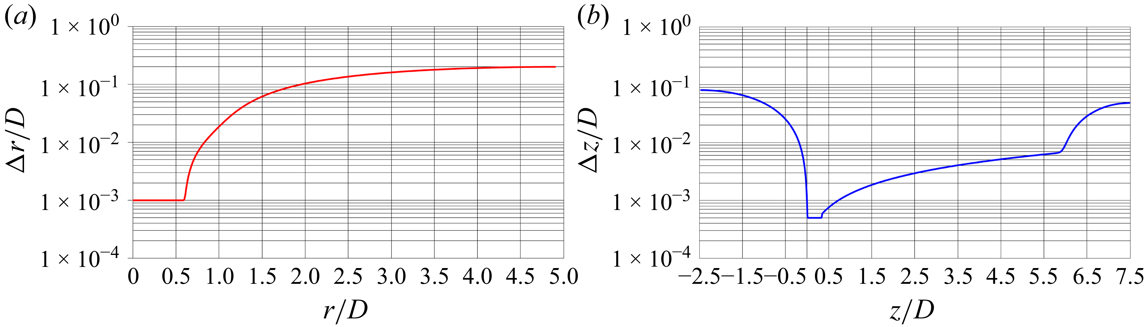


 MOD

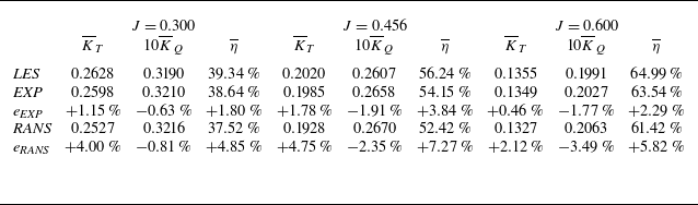
 REF
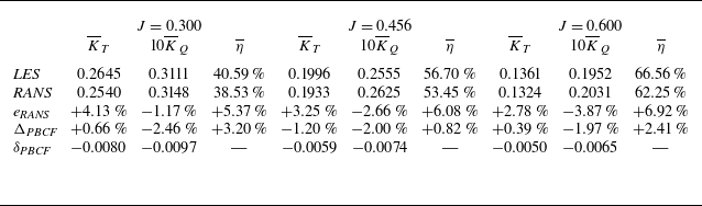
 MOD
 REF

 REF
 MOD
 J=0.300
 J=0.456
 J=0.600

 MOD
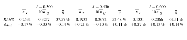
 REF
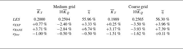
 REF
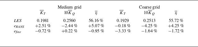
 MOD

 0.0
 0.2

 REF
 MOD
 U/D
 J=0.300
 cp=−5.0
 J=0.456
 cp=−1.5
 J=0.600
 cp=−0.3

 REF
 MOD
 U/D
 J=0.300
 Q^D2/U2=500
 J=0.456
 Q^D2/U2=200
 J=0.600
 Q^D2/U2=50
 Q^

 U/D
 J=0.300
 REF
 MOD
 z/D=0.25
 z/D=0.30
 z/D=0.35
 z/D=0.40
 z/D=0.45

 U2
 J=0.300
 REF
 MOD
 z/D=0.25
 z/D=0.30
 z/D=0.35
 z/D=0.40
 z/D=0.45

 REF
 MOD
 U/D
 J=0.300
 cp=−1.00
 J=0.456
 cp=−0.20
 J=0.600
 cp=−0.05
 0.0

 REF
 MOD
 U/D
 J=0.300
 QD2/U2=10000
 J=0.456
 QD2/U2=2000
 J=0.600
 QD2/U2=1000
 Q

 z/D=0.5
 J=0.456

 z/D=0.5
 J=0.300

 z/D=0.5
 J=0.600

 J=0.300
 J=0.456
 J=0.600
 r/D=0.0
 r/D=0.2

 U
 J=0.456
 REF
 MOD
 w¯=0

 U/D
 U2/D2
 J=0.456
 REF
 MOD
 w¯=0

 U/D
 U2/D2
 J=0.300
 REF
 MOD
 w¯=0

 U/D
 U2/D2
 J=0.600
 REF
 MOD
 w¯=0

 J=0.300
 J=0.456
 J=0.600
 r/D=0.00
 r/D=0.02

 U2
 J=0.456
 REF
 MOD

 U2
 J=0.300
 REF
 MOD

 U2
 J=0.600
 REF
 MOD

 z/D=0.5
 z/D=3.0
 J=0.300
 J=0.456
 J=0.600

 J=0.300
 J=0.456
 J=0.600
 0.0

 z/D=0.5
 z/D=3.0
 J=0.300
 J=0.456
 J=0.600

 J=0.300
 J=0.456
 J=0.600
 0.0

 Open access

