1. Introduction
Buoyancy-driven turbulent convection subject to background rotation is a ubiquitous phenomenon in geophysics and astrophysics. For instance, the renowned tropical circulation in Earth’s atmosphere, known as the Hadley cell, is a result of the interplay between buoyancy and rotation. A widely employed model for investigating these flows is rotating Rayleigh–Bénard convection (RRBC), where a rotating fluid layer is heated from below and cooled from above (Ecke & Shishkina Reference Ecke and Shishkina2023). In RRBC, the strength of the buoyancy force is quantified by the Rayleigh number
 $Ra=\alpha g \Delta T H^{3}/(\nu \kappa )$
. Rotation introduces two additional forces in the RRBC system: the Coriolis force and the centrifugal force. The significance of the Coriolis force can be assessed using the Ekman number
 $Ek = \nu /(2\varOmega H^{2})$
or the Rossby number
 $\textit{Ro}=U_{\!\textit{ff}}/(2\varOmega H)$
, while the centrifugal force is quantified by the Froude number
 $\textit{Fr}=\varOmega ^{2}R/g$
. Here,
 $\alpha$
,
 $\nu$
and
 $\kappa$
represent the thermal expansion coefficient, kinematic viscosity and thermal diffusivity of the working fluid, respectively;
 $\Delta T$
corresponds to the temperature difference across the fluid layer,
 $\varOmega$
denotes the rotation speed antiparallel to the gravity
 $g$
, and
 $U_{\!\textit{ff}}=\sqrt {\alpha g \Delta T H}$
is the free-fall velocity. The remaining control parameters include the Prandtl number
 $\textit{Pr}=\nu /\kappa$
and the diameter-to-height aspect ratio
 $\varGamma = 2R/H$
, with
 $R$
and
 $H$
the radius and height of the flow domain, respectively.
Compared to the centrifugal effect, the Coriolis effect has garnered significant attention (see e.g. Kunnen Reference Kunnen2021; Ecke & Shishkina Reference Ecke and Shishkina2023). The most obvious example is the famous Taylor–Proudman (TP) effect, which could result in two-dimensional columnar structures in the flow fields. In RRBC without centrifugal force, convection initiates once the Rayleigh number
 $Ra$
exceeds a critical value
 $Ra_c=A\textit{Ek}^{-4/3}$
, where the coefficient is
 $A=8.70-9.63\textit{Ek}^{1/6}$
(Niiler & Bisshopp Reference Niiler and Bisshopp1965), and its asymptotic value for an infinite fluid layer is 8.7 (Chandrasekhar Reference Chandrasekhar1981). With
 $Ra\gt Ra_c$
, the increased buoyancy force breaks the TP constraint, resulting in various flow states with different flow structures that depend on
 $\textit{Pr}$
(Sprague et al. Reference Sprague, Julien, Knobloch and Werne2006; Julien et al. Reference Julien, Rubio, Grooms and Knobloch2012; Nieves, Rubio & Julien Reference Nieves, Rubio and Julien2014). For the flow with
 $\textit{Pr}\gtrsim 2$
(Kunnen Reference Kunnen2021), the laminar vortical columns arrange themselves in a steady grid in the cells regime with
 $Ra/Ra_c\gtrsim 1$
, which are soon replaced by disordered columns in the convective Taylor column (CTC) regime at larger
 $Ra/Ra_c$
. Then in the plume regime, the strong interactions between columns cause them to break down into shorter vortical structures. Finally, the flow becomes turbulent in the geostrophic turbulence regime.
Recently, there has been increasing attention given to the centrifugal effect in RRBC. Theoretical analysis has shown that centrifugal force breaks the top-down symmetry of the system, and can lead to the accumulation of hot fluid at cell centre (e.g. Lopez, Rubio & Marques Reference Lopez, Rubio and Marques2006). Since centrifugal force is inevitably present in experiments, the time when these centrifugal effects become non-negligible becomes an important issue. A criterion
 $\textit{Fr}\sim 0.05$
was first adopted in early works (e.g. Marques et al. Reference Marques, Mercader, Batiste and Lopez2007). However, after a new critical Froude number
 $\textit{Fr}_c^{\textit{global}}=\varGamma /2$
was introduced in the inspiring work of Horn & Aurnou (Reference Horn and Aurnou2018),
 $\textit{Fr}_c^{\textit{global}}$
was then widely used as a new criterion. Later in our recent paper (Hu, Xie & Xia Reference Hu, Xie and Xia2022), the meanings of these two Froude numbers are clarified;
 $\textit{Fr}\sim 0.05$
is the onset Froude number, beyond which the centrifugal effect starts to manifest itself. And it is further found from bulk temperature measurements that this onset value is not a constant; it scales with
 $Ra$
as
 $\textit{Fr}_c^{\textit{local}}\sim Ra^{0.53}$
(Hu et al. Reference Hu, Xie and Xia2022). On the other hand,
 $\textit{Fr}_c^{\textit{global}}$
is the critical value beyond which the centrifugal force is strong enough to dominate the flow dynamics (Horn & Aurnou Reference Horn and Aurnou2018). Therefore, the regime with
 $\textit{Fr}\gt \textit{Fr}_c^{\textit{global}}$
was regarded as the strong centrifugal (SC) regime, whereas the one with
 $\textit{Fr}_c^{\textit{local}} {} \lt Fr\lt \textit{Fr}_c^{\textit{global}}$
is the weak centrifugal (WC) regime (Hu et al. Reference Hu, Xie and Xia2022).
The centrifugal effect in the SC regime has been studied in great detail (Horn & Aurnou Reference Horn and Aurnou2019, Reference Horn and Aurnou2021). Briefly, it pushes the hot (cold) fluid parcels towards the centre (sidewall) along the hot (cold) plate, forming a hot (cold) coherent structure. Nevertheless, it behaves entirely differently when the centrifugal force is much weaker and the flow is full of columns (Noto et al. Reference Noto, Tasaka, Yanagisawa and Murai2019; Ding et al. Reference Ding, Chong, Shi, Ding, Lu, Xia and Zhong2021). For example, with the WC force, the horizontal dynamics of these columns changes from sub-diffusive at short-time scales to super-diffusive at long-time scales (Noto et al. Reference Noto, Tasaka, Yanagisawa and Murai2019). Besides these effects, how the RRBC system responds to the WC force in the WC regime is still ambiguous, which motivates us to explore this regime more deeply in this study.
The critical Froude number
 $\textit{Fr}_c^{\textit{global}}$
introduced by Horn & Aurnou (Reference Horn and Aurnou2018) was obtained from global dimensional arguments. By considering the balance between the free-fall time scale
 $\tau _{f\!f}=[H/(\alpha g \Delta T)]^{1/2}$
and the centrifugal buoyancy time scale
 $\tau _{cb}=[R/(\alpha \varOmega ^2R \Delta T)]^{1/2}$
, it becomes evident that
 $\textit{Fr}_c^{\textit{global}}=\varGamma /2$
. The similarity between the definitions of
 $\tau _{f\!f}$
and
 $\tau _{cb}$
implies the assumption that the horizontal dynamics of a fluid parcel is also free-fall under the ‘horizontal gravity’
 $\varOmega ^2R$
over the global horizontal scale
 $R$
. However, when the flow is full of columns, the horizontal dynamics is most likely to be diffusive. So it is better to assume that only within a local length scale
 $\ell$
(analogous to the mean free path in ideal gas systems) can the horizontal dynamics be regarded as free-fall. This mechanism of local dynamics has been introduced to understand the scaling
 $\textit{Fr}_c^{\textit{local}}\sim Ra^{0.53}$
qualitatively (Hu et al. Reference Hu, Huang, Xie and Xia2021, Reference Hu, Xie and Xia2022). In this paper, this idea is developed further to provide a quantitative explanation for
 $\textit{Fr}_c^{\textit{local}}$
.
The remainder of this paper is organised as follows. The experimental set-up and the parameters are introduced in § 2. For the results, the respective centrifugal effects on the bulk flow and sidewall boundary flow in the WC regime are revealed in § 3. In the following section, discussing the onset Froude number
 $\textit{Fr}_c^{\textit{local}}$
, the mechanism of local force balance is first explained in detail, which is then used to understand the behaviour of
 $\textit{Fr}_c^{\textit{local}}$
. Finally, we summarise our findings in § 5.
2. Experimental set-up and the parameters
2.1. Experimental set-up
The experimental set-ups used for heat transport (i.e. the Nusselt number
 $\textit{Nu}$
) and flow field measurements are identical to those in Sun et al. (Reference Sun, Hu, Wang and Xia2024). The cell for
 $\textit{Nu}$
measurements comprises two copper plates with a plexiglass tube sandwiched between them. The cell has height
 $H=96.15$
mm and diameter
 $2R=191.95$
mm, yielding aspect ratio
 $\varGamma =2R/{} H=2$
. The heat flux
 $q$
is introduced to the bottom hot plate by heating wires, and then removed by the top cold plate. The temperatures of the hot plate (
 $T_h$
) and cold plate (
 $T_c$
) are measured using four thermistors in each plate. The temperature difference
 $\Delta T=T_h-T_c$
across the fluid layer covers the range
 $1.0\leqslant \Delta T\leqslant 22.6$
K. The working fluid, i.e. degassed and deionised water, is kept at a constant mean temperature
 $T_m=(T_h+T_c)/2=40.0\,^{\circ}\text{C}$
, resulting in Prandtl number
 $\textit{Pr}=4.34$
. Together with the Nusselt number
 $\textit{Nu}$
, the bulk temperature
 $T_b$
is simultaneously measured by positioning a small thermistor at the cell centre. The sidewall temperature
 $T_w$
is also monitored, by inserting several thermistors into blind holes in the sidewall. These thermistors are divided into three layers at heights
 $H/4$
,
 $H/2$
and
 $3H/4$
from the bottom plate. Each layer contains eight thermistors distributed azimuthally at equal intervals. All the temperature signals are sampled for at least four hours after the system reaches a stable state.
For particle image velocimetry (PIV) measurements, a hot plate coated with black nickel is utilised to minimise the influence of reflected laser on the images. Additionally, a rectangular jacket, also filled with degassed and deionised water, is fitted outside the cylindrical sidewall to prevent optical distortion. The vertical flow field along the cell’s centreline is illuminated by a continuous 532 nm laser, and recorded for 20 min by an iDS camera with resolution 2048
 $\times$
1024 pixels and frequency
 $\sim10$
Hz. For the horizontal flow field measurements at height
 $z=H/4$
, the copper top plate is further replaced by a sapphire plate, above which is a transparent water chamber. The circulating water from a temperature-controlled water bath is pumped into this chamber to remove heat flux. The horizontal fields are recorded by a high-performance CMOS camera (FLIR.ORX-10G, resolution 3000
 $\times$
3000 pixels) for one hour at frequency 2–20 Hz, depending on
 $Ra/Ra_c$
. Velocity vectors are calculated using commercial PIV processing software (LaVision), with a 32
 $\times$
32 pixels interrogation window and a
 $50\,\%$
overlap between neighbouring windows.
2.2. Parameter space
During the experiments, the temperature difference
 $\Delta T$
is fixed, and for each fixed
 $\Delta T$
, the rotation rate
 $\varOmega$
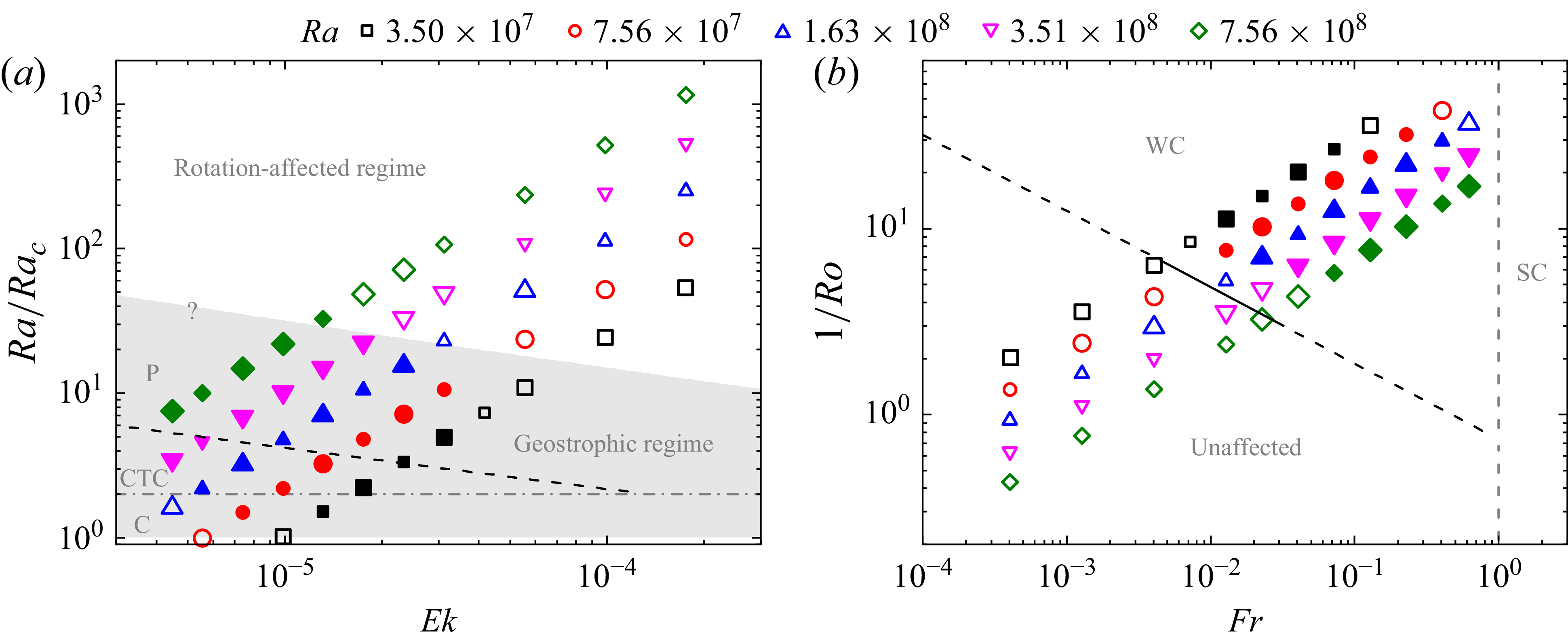
is varied from 1.9 rpm to 76.0 rpm. A total of five data sets are collected. The corresponding control parameters are depicted in figure 1, and more details can be found in Appendix A.
(a) The space of
 $Ra/Ra_c{-}Ek$
, which is divided into a rotation-affected regime and a geostrophic regime (the shaded area). The latter regime can be further divided into several sub-regimes, i.e. the cells (C), the CTC and the plumes (P) regimes, which are separated by the dash-dotted line
 $Ra/Ra_c=2$
(Julien et al. Reference Julien, Rubio, Grooms and Knobloch2012) and the black dashed line
 $Ra\,\textit{Ek}^{1.66}=0.71$
(Sun et al. Reference Sun, Hu, Wang and Xia2024), respectively. (b) The space of
 $1/Ro{-}Fr$
is divided into a regime unaffected by the centrifugal force, a WC regime and an SC regime. The vertical dashed line is
 $\textit{Fr}_c^{\textit{global}}=\varGamma /2$
(Horn & Aurnou Reference Horn and Aurnou2018), and the black solid line is
 $\textit{Fr}_c^{\textit{local}}=3.19\times 10^{-7}Ra^{0.55}$
(see figure 6), which is extrapolated to larger and smaller Froude numbers (the black dashed lines). In both spaces, heat transfer efficiency and temperature signals are measured for all the symbols. The solid symbols (the symbols with larger size) are the cases where the horizontal flow fields at
 $z=H/4$
(the vertical fields) are also measured by PIV.

The
 $Ra/Ra_c{-}Ek$
parameter space in figure 1(a) is utilised to investigate the Coriolis effect. According to Kunnen (Reference Kunnen2021), this space can be divided into two regimes, i.e. the rotation-affected regime and the geostrophic regime (shaded area), and the separation between them is difficult to determine precisely. The geostrophic regime can be further divided into several sub-regimes, namely, the cells (C), CTC and plume (P) regimes. The transition from the cells regime to the CTC regime occurs at
 $Ra/Ra_c=2$
(grey dash-dotted line) (Julien et al. Reference Julien, Rubio, Grooms and Knobloch2012), while the CTC and plume regimes are separated by the black dashed line
 $Ra\,\textit{Ek}^{1.66}=0.71$
(Sun et al. Reference Sun, Hu, Wang and Xia2024). The centrifugal effect is investigated in the
 $1/Ro{-}Fr$
space (figure 1
b), which can be divided into three regimes: a regime unaffected by the centrifugal force, a WC regime and an SC regime (Hu et al. Reference Hu, Xie and Xia2022). The vertical grey dashed line separating the WC and SC regimes represents the critical Froude number
 $\textit{Fr}_c^{\textit{global}}=\varGamma /2$
(Horn & Aurnou Reference Horn and Aurnou2018). The black solid line corresponds to the onset Froude number
 $\textit{Fr}_c^{\textit{local}}=3.19\times 10^{-7}Ra^{0.55}$
, which is extrapolated to larger and smaller Froude numbers (the black dashed lines). As can be seen from figure 1(b),
 $\textit{Fr}$
and
 $\textit{Ro}$
(or
 $Ek$
) are covaried in the present experiments.
In figure 1, all the symbols represent the cases where heat transport and temperature signals are measured. Among these symbols, the solid ones indicate the cases where the horizontal flow fields at height
 $z=H/4$
are measured, and the symbols with larger size represent cases where the vertical flow fields are measured.
3. The WC effects
How the WC force manifests itself in the WC regime may become an important issue in experiments, since one needs to find out to what degree the statistics are affected by the unavoidable centrifugal force. To address this question, the bulk flow and the sidewall flow are investigated separately below.
3.1. The WC effects on the bulk flow
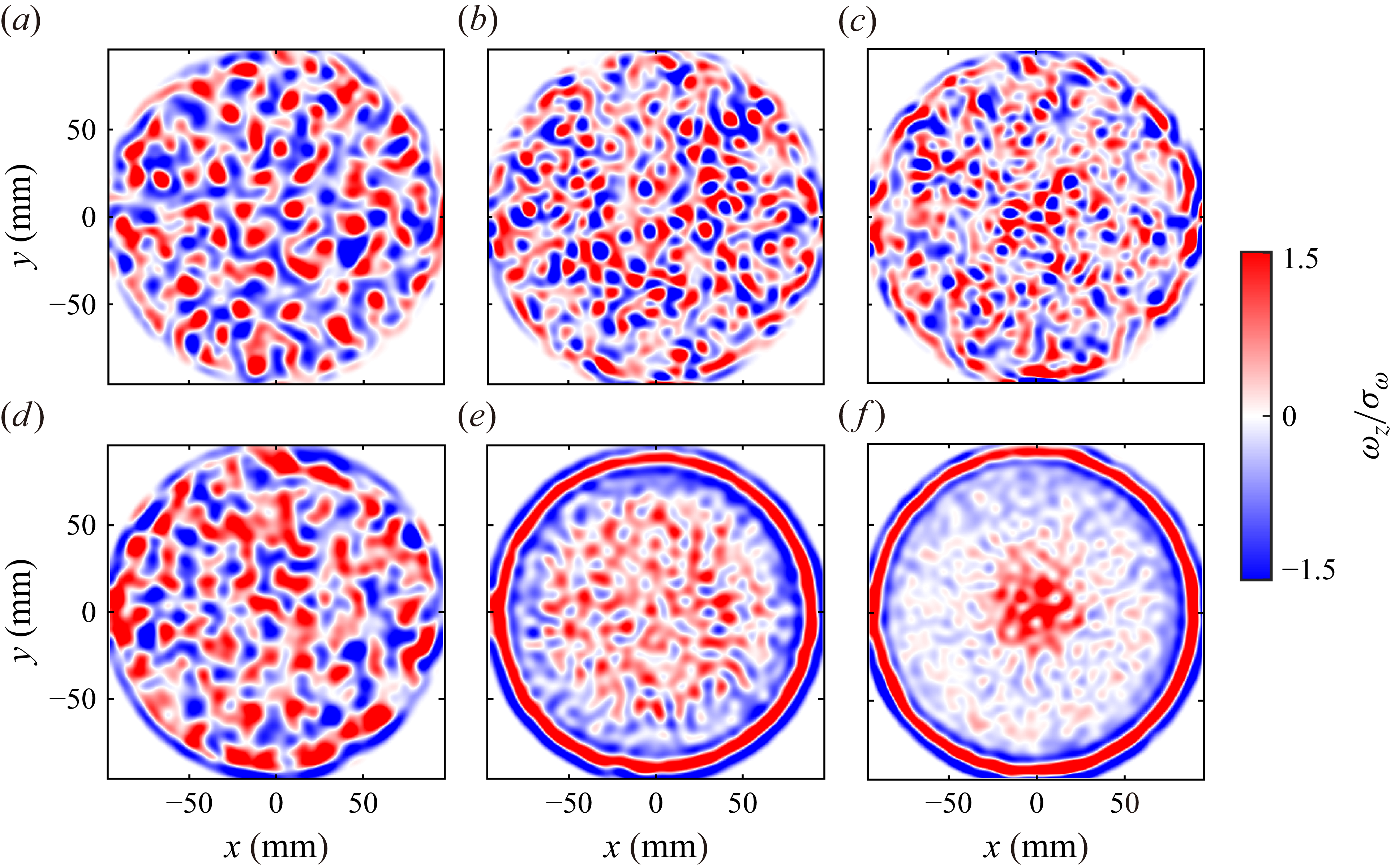
We first evaluate the WC effect on the bulk flow, by examining the overall flow fields in figure 2. Figures 2(a–c) are instantaneous vertical vorticity fields
 $\omega _z$
. It can be seen that although the Froude number has increased significantly from
 $0.072$
to
 $0.405$
in these three cases, the centrifugal force is still not strong enough to change the morphology of flow structures. That is, a large hot coherent structure as shown in Horn & Aurnou (Reference Horn and Aurnou2019) does not emerge in the bulk region, and individual columns can still be recognised. Actually, it has been proved that the WC force has negligible effect on these instantaneous flow fields (Sun et al. Reference Sun, Hu, Wang and Xia2024). However, the situation becomes different for long-time averaged vorticity fields (figures 2
d–f). Since these horizontal fields are measured at height
 $z=H/4$
, regions with positive (negative) vorticity should correspond to hot (cold) structures in the present experiments. It can be seen that the hot fluid parcels accumulate at cell centre, and this feature becomes more pronounced at larger centrifugal force.
Examples of vertical vorticity fields
 $\omega _z$
for
 $Ra=1.63\times 10^{8}$
: (a–c) instantaneous fields, (d–f) long-time averaged fields. The corresponding parameters
 $Ra/Ra_c$
,
 $\textit{Fr}$
,
 $\textit{Ro}$
,
 $Ek$
are, respectively, (a,d)
 $7.03,\ 0.072,\ 0.081,\ 1.32\times 10^{-5}$
, (b,e)
 $3.20,\ 0.228,\ 0.045,\ 7.41\times 10^{-5}$
and (c, f)
 $2.16,\ 0.405,{} 0.034,\ 5.55\times 10^{-6}$
.

As it is impractical to make PIV measurements for all cases, we turn to bulk temperatures
 $T_b$
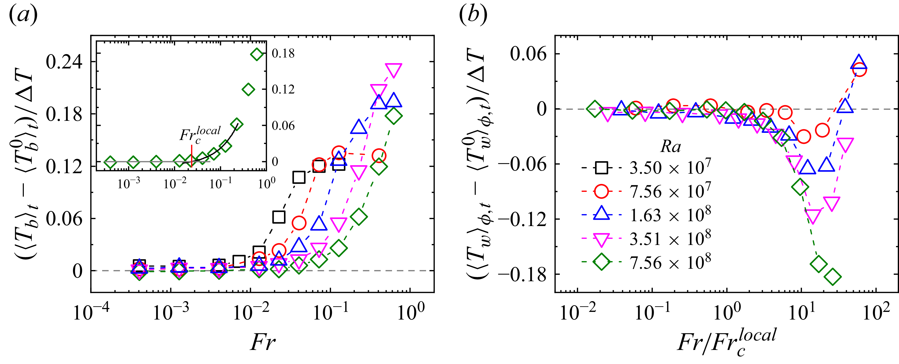
for longer-term measurements in order to reveal more quantitative information. In figure 3(a), the time-averaged bulk temperatures
 $\langle T_b \rangle _t$
for various
 $Ra$
are plotted relative to the respective baselines
 $\langle T_b^0\rangle _t$
for better comparison. Here,
 $\langle T_b^0\rangle _t$
is the mean bulk temperature without rotation, which, due to the non-Oberbeck–Boussinesq (NOB) effect, is larger for larger
 $Ra$
(Ahlers et al. Reference Ahlers, Brown, Araujo, Funfschilling, Grossmann and Lohse2006). It can be seen that for each
 $Ra$
, the bulk temperature anomaly starts to increase when
 $\textit{Fr}$
exceeds an onset value
 $\textit{Fr}_c^{\textit{local}}$
, and it appears to saturate at large
 $\textit{Fr}$
for some cases. All these features agree well with previous studies (Horn & Aurnou Reference Horn and Aurnou2019; Hu et al. Reference Hu, Xie and Xia2022). Numerical simulations have proved that the NOB effect under rotation would result in a bulk temperature
 $\langle T_b\rangle _t$
smaller than its non-rotation value
 $\langle T_b^0\rangle _t$
(Horn & Shishkina Reference Horn and Shishkina2014). Therefore, the increased bulk temperature anomaly is a manifestation of centrifugal effect at large
 $\textit{Fr}\gt \textit{Fr}_c^{\textit{local}}$
, which is consistent with the findings of accumulated hot fluids at cell centre revealed by PIV results in figure 2. The onset Froude number
 $\textit{Fr}_c^{\textit{local}}$
is determined by intersecting a linear fitting of the increased data and a baseline (inset of figure 3
a), which shows a 0.55 scaling on
 $Ra$
(see figure 6). Note that a 0.53 scaling also obtained from
 $T_b$
has been reported in Hu et al. (Reference Hu, Xie and Xia2022), but the data here are with much higher accuracy, and the Rayleigh number here is extended to approximately a decade wider, indicating the robustness of the results.
(a) The normalised time-averaged bulk temperatures
 $\langle T_b \rangle _t / \Delta T$
are plotted relative to the corresponding non-rotation values
 $\langle T_b^0\rangle _t$
as functions of
 $\textit{Fr}$
. The inset exemplifies how the onset Froude number
 $\textit{Fr}_c^{\textit{local}}$
is obtained. (b) The normalised temporally and azimuthally averaged sidewall temperatures
 $\langle T_w \rangle _{\phi ,t} / \Delta T$
are plotted relative to the corresponding non-rotation values
 $\langle T_w^0\rangle _{\phi ,t}$
as functions of
 $\textit{Fr}/\textit{Fr}_c^{\textit{local}}$
. Note that the data for
 $Ra=3.50\times 10^7$
(corresponding to
 $\Delta T=1.0$
K) are not shown (see text).

In the above, we have shown that the WC force cannot affect the instantaneous fields, but its effect on long-time averaged ones is significant. These different behaviours can be understood as follows. The results reported by Noto et al. (Reference Noto, Tasaka, Yanagisawa and Murai2019) have shown that for the short-time-scale dynamics of columns, the WC effect is not significant, whereas over a long-time scale, the columns slowly accelerate radially due to the WC force. This directed motion on average implies that the probability of finding hot columns at cell centre is larger than for cold ones, resulting in a hotter bulk flow on mean fields.
3.2. The WC effects on the sidewall flow
The ring structures near the sidewall in figures 2(e, f) indicate a complex flow state there. Before diving deeper into the issue about the centrifugal effect on these sidewall flows, let us first uncover an interesting phenomenon concealed within previous results. As found in previous studies, the case without centrifugal force (i.e.
 $\textit{Fr}=0$
) exhibits a cyclonic boundary zonal flow (BZF) near the sidewall, accompanied with an anticyclonic bulk flow (Zhang et al. Reference Zhang, Van Gils, Horn, Wedi, Zwirner, Ahlers, Ecke, Weiss, Bodenschatz and Shishkina2020, Reference Zhang, Ecke and Shishkina2021; Wedi et al. Reference Wedi, Moturi, Funfschilling and Weiss2022). Nevertheless, for the case with very large
 $\textit{Fr}$
, the converging hot fluids along the bottom plate evolve into a cyclonic bulk flow due to the additional Coriolis effect, and similarly, the diverging cold fluids form an anticyclonic sidewall flow (Horn & Aurnou Reference Horn and Aurnou2018). Therefore, for these two extreme cases (i.e.
 $\textit{Fr}=0$
versus large
 $\textit{Fr}$
), the azimuthal motions of the sidewall and bulk flows are opposite.
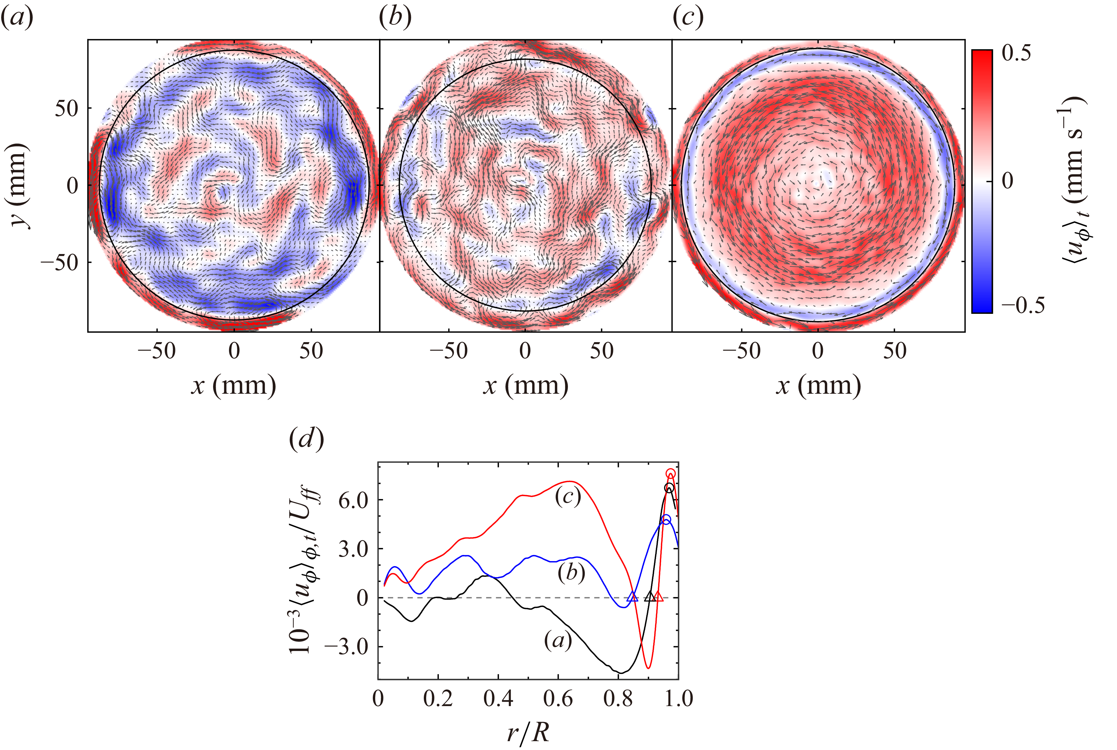
Typical examples of mean azimuthal velocity fields
 $\langle u_\phi \rangle _t$
measured at
 $z=H/4$
for
 $Ra=1.63\times 10^8$
. The parameters
 $Ra/Ra_c, Fr, Ro, Ek$
are, respectively, (a)
 $15.46,\ 0.023,\ 0.144,\ 2.34\times 10^{-5}$
, (b)
 $7.03,\ 0.072,\ 0.081,\ 1.32\times 10^{-5}$
and (c)
 $3.20,\ 0.228,\ 0.045,\ 7.41\times 10^{-5}$
. The black solid line in each panel indicates the position of BZF. (d) The corresponding radial profiles. The open triangles are the positions
 $r=r_0$
of the first zero-crossing from the sidewall, and open circles indicate the maxima
 $u_\phi ^{max}$
near the sidewall at positions
 $r=r_{\textit{max}}$
.

Figure 3(b) shows the temporally and azimuthally averaged sidewall temperatures
 $\langle T_w \rangle _{\phi ,t}$
. Here, the data for
 $Ra=3.50\times 10^7$
(corresponding to
 $\Delta T=1.0$
K) are not shown, since the temperature signals indirectly measured inside the sidewall can be easily affected by fluctuating surroundings. It can be seen that
 $\langle T_w \rangle _{\phi ,t}$
starts to decrease once
 $\textit{Fr}$
exceeds
 $\textit{Fr}_c^{\textit{local}}$
, indicating the effect of centrifugal force. However, it goes up again at larger
 $\textit{Fr}$
, the reason for which is not clear yet. Here, it is worth mentioning that the complex behaviours of
 $\langle T_w \rangle _{\phi ,t}$
shown within the
 $1/Ro{-}Fr$
space by Horn & Aurnou (Reference Horn and Aurnou2019) also imply that
 $\langle T_w \rangle _{\phi ,t}$
does not monotonically decrease if increasing
 $\textit{Fr}$
meanwhile keeping
 $Ra$
fixed (refer to figure 7(b) therein). In any case, the behaviours of
 $\langle T_w \rangle _{\phi ,t}$
at
 $\textit{Fr}\gt \textit{Fr}_c^{\textit{local}}$
suggest that the centrifugal force has come into effect, from which an anticyclonic sidewall flow should be expected. On the other hand, according to Zhang, Ecke & Shishkina (Reference Zhang, Ecke and Shishkina2021) and Wedi et al. (Reference Wedi, Moturi, Funfschilling and Weiss2022), for the present parameters, a cyclonic BZF should develop near the sidewall. To understand whether the dynamics of the sidewall flow is dominated by BZF or by centrifugal force, we plot mean azimuthal velocities
 $\langle u_\phi \rangle _t$
in figure 4. It can be seen that when the centrifugal force is very weak, the bulk (sidewall) region is dominated by an anticyclonic (cyclonic) flow (figure 4
a), which is similar to the BZF case. However, at larger
 $\textit{Fr}=0.072$
in figure 4(b), the bulk flow changes to cyclonic flow while the boundary flow still remains cyclonic, and this feature becomes more pronounced at even larger
 $\textit{Fr}$
in figure 4(c). Interestingly, an anticyclonic band separating the bulk and boundary cyclonic flows develops in figure 4(c). We found that this band vanishes gradually when
 $\textit{Fr}$
increases further. These results suggest that although the bulk flow is significantly affected by the centrifugal force, the sidewall flow is otherwise still dominated by BZF.
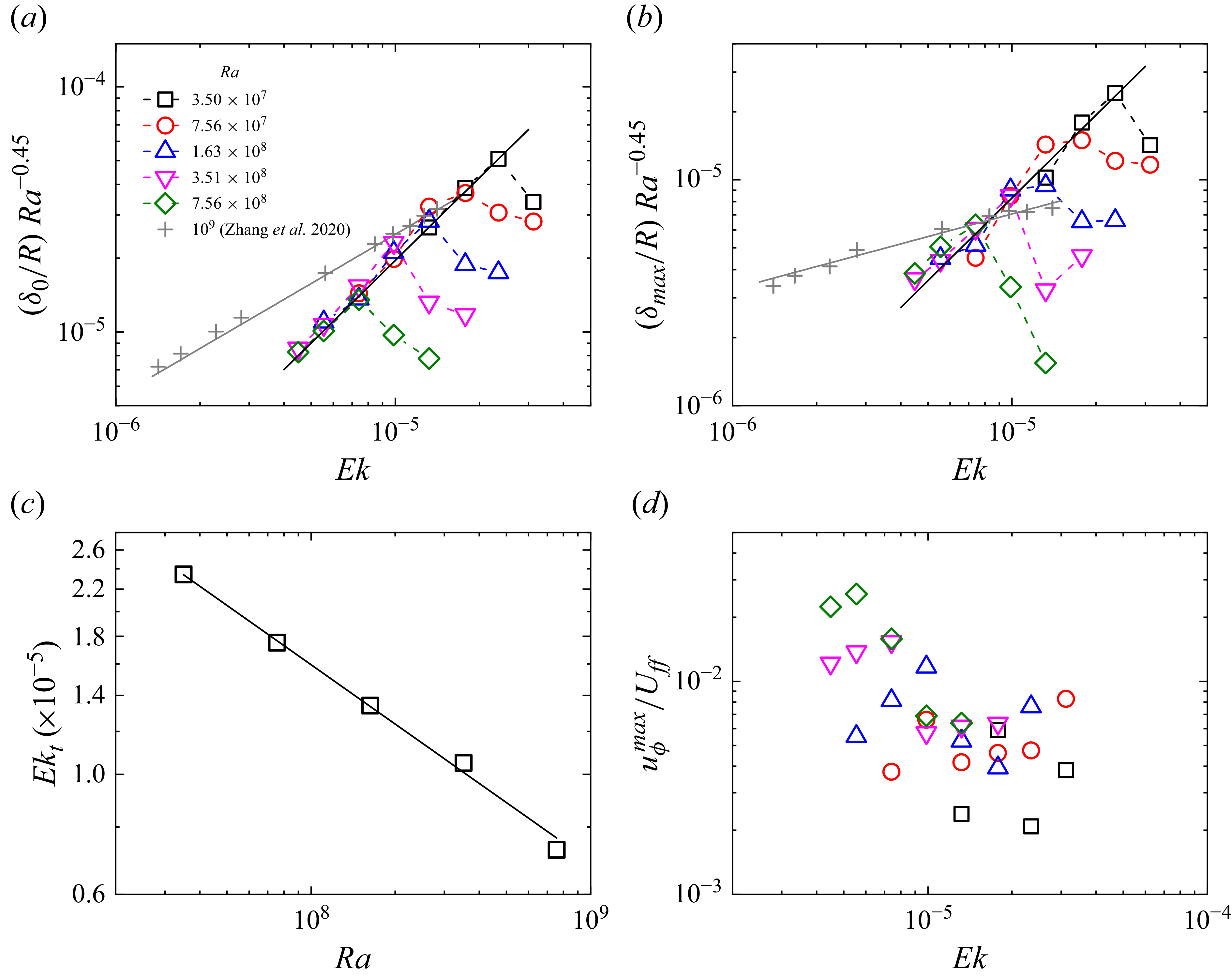
(a) The width of BZF
 $\delta _0$
. The black solid line is a power-law fitting
 $\delta _0/R=7.8\,Ra^{0.45}\,\textit{Ek}^{1.12}$
to the data before the transitional Ekman number
 $Ek_t$
, where a sharp decrement occurs. The grey pluses are from Zhang et al. (Reference Zhang, Van Gils, Horn, Wedi, Zwirner, Ahlers, Ecke, Weiss, Bodenschatz and Shishkina2020) for
 $Ra=10^9$
, which exhibit a two-thirds scaling
 $\delta _0/R\sim \textit{Ek}^{2/3}$
(the grey solid line). (b) Similar plot for the velocity layer
 $\delta _{\textit{max}}$
. Black solid line:
 $\delta _{\textit{max}}/R=10.47\,Ra^{0.45}\,\textit{Ek}^{1.22}$
. Grey solid line:
 $\delta _{\textit{max}}/R\sim \textit{Ek}^{1/3}$
(Zhang et al. Reference Zhang, Van Gils, Horn, Wedi, Zwirner, Ahlers, Ecke, Weiss, Bodenschatz and Shishkina2020). (c) The transitional Ekman number
 $Ek_t$
follows a power-law scaling
 $Ek_t=0.013\,Ra^{-0.36\pm 0.01}$
(the black solid line). (d) Normalised maximum azimuthal velocity
 $u_\phi ^{max}$
plotted against
 $Ek$
.

In figure 5, more quantitative results on BZF are displayed. In order to make more direct comparison with results from previous studies, the width of BZF is also defined from the mean azimuthal velocity profile as
 $\delta _0\equiv R-r_0$
, where
 $r=r_0$
is the radial position of the first zero-crossing from the sidewall (Zhang et al. Reference Zhang, Van Gils, Horn, Wedi, Zwirner, Ahlers, Ecke, Weiss, Bodenschatz and Shishkina2020). The strength of BZF is quantified by the maximum value
 $u_\phi ^{max}$
of mean azimuthal velocity at
 $r=r_{\textit{max}}$
, from which another width of velocity layer
 $\delta _{\textit{max}}\equiv R-r_{\textit{max}}$
can be obtained. Figure 4(d) illustrates how these quantities are defined.
Let us first look at the normalised width
 $\delta _0/R$
of BZF in figure 5(a). It can be seen that for each
 $Ra$
, there is a sharp decrease of
 $\delta _0/R$
at some transitional Ekman number
 $Ek_t$
, which is found to follow a well-defined power-law scaling
 $Ek_t=0.013\,Ra^{-0.36\pm 0.01}$
(figure 5
c). After a closer check of the flow fields, we found that for the cases with
 $Ek\gt Ek_t$
, the BZF is not well developed (e.g. figure 4
a). This behaviour is qualitatively in agreement with the experimental findings reported by Wedi et al. (Reference Wedi, Moturi, Funfschilling and Weiss2022), who also found a drop of
 $\delta _0/R$
at large
 $Ek$
. A direct two-dimensional fitting to the data with
 $Ek\leqslant Ek_t$
yields
 $\delta _0/R = 7.8\,Ra^{0.45\pm 0.03}\,\textit{Ek}^{1.12\pm 0.09}$
. In figure 5(a), the
 $Ra$
dependence is compensated to show the Ekman scaling more clearly, which differs a lot from the two-thirds scaling reported by Zhang et al. (Reference Zhang, Van Gils, Horn, Wedi, Zwirner, Ahlers, Ecke, Weiss, Bodenschatz and Shishkina2020, Reference Zhang, Ecke and Shishkina2021). Similar behaviours can be observed for
 $\delta _{\textit{max}}$
(figure 5
b). The scaling for the data before transition is
 $\delta _{\textit{max}}/R = 10.47\,Ra^{0.45\pm 0.05}\,\textit{Ek}^{1.22\pm 0.07}$
. This 1.22 scaling on
 $Ek$
is much larger than the one-third scaling presented by Zhang et al. (Reference Zhang, Van Gils, Horn, Wedi, Zwirner, Ahlers, Ecke, Weiss, Bodenschatz and Shishkina2020, Reference Zhang, Ecke and Shishkina2021) and the one-half scaling estimated by Wedi et al. (Reference Wedi, Moturi, Funfschilling and Weiss2022). As for the strength of BZF, scalings
 $u_\phi ^{max}\sim \textit{Ek}^{2/3}$
and
 $u_\phi ^{max}\sim \textit{Ek}^{3/2}$
were reported, respectively, by Zhang et al. (Reference Zhang, Ecke and Shishkina2021) and Wedi et al. (Reference Wedi, Moturi, Funfschilling and Weiss2022). In figure 5(d), the present data are too scattering to reveal a scaling, but the decreasing trend with increasing
 $Ek$
can be easily observed, which is entirely different from these two reported scalings.
The underlying reasons for these huge differences are unclear to us. Although the covered parameter ranges of
 $Ra$
and
 $Ek$
between the present study and previous ones are different, this may not be the key factor. For example, the results in Wedi et al. (Reference Wedi, Moturi, Funfschilling and Weiss2022) are in the rotation-affected regime, and the work in Zhang et al. (Reference Zhang, Ecke and Shishkina2021) covers the geostrophic regime, but the overall behaviours of the statistics about BZF are similar, especially for the scalings of
 $\delta _0$
(see figure 5(b) in Wedi et al. Reference Wedi, Moturi, Funfschilling and Weiss2022). As for the aspect ratio
 $\varGamma$
, the BZF statistics in Zhang et al. (Reference Zhang, Ecke and Shishkina2021) show no
 $\varGamma$
dependence within the range
 $1/3\leqslant \varGamma \leqslant 2$
. Therefore, the aspect ratio may also have negligible effects on the observed differences in figure 5. Note that the centrifugal force is not considered by Zhang et al. (Reference Zhang, Ecke and Shishkina2021) in their numerical studies. As for the experiments in Wedi et al. (Reference Wedi, Moturi, Funfschilling and Weiss2022), the centrifugal effect is also insignificant, since even for their fastest rotation speed (i.e. lowest
 $Ek=1.6\times 10^{-5}$
at
 $Ra=9.8\times 10^8$
), the Froude number
 $\textit{Fr}=0.024$
is just a little above the onset value
 $\textit{Fr}_c^{\textit{local}}=0.022$
(estimated with the
 $\varGamma =1$
scaling
 $\textit{Fr}_c^{\textit{local}}=3.79\times 10^{-7}Ra^{0.53}$
; see figure 6
a). These observations, together with the decreased sidewall temperatures in figure 3(b), imply that the most probable reason for the above differences is the influence of centrifugal force. The underlying mechanism for how the centrifugal force modifies the sidewall flows, especially on the properties of BZF, needs further study.
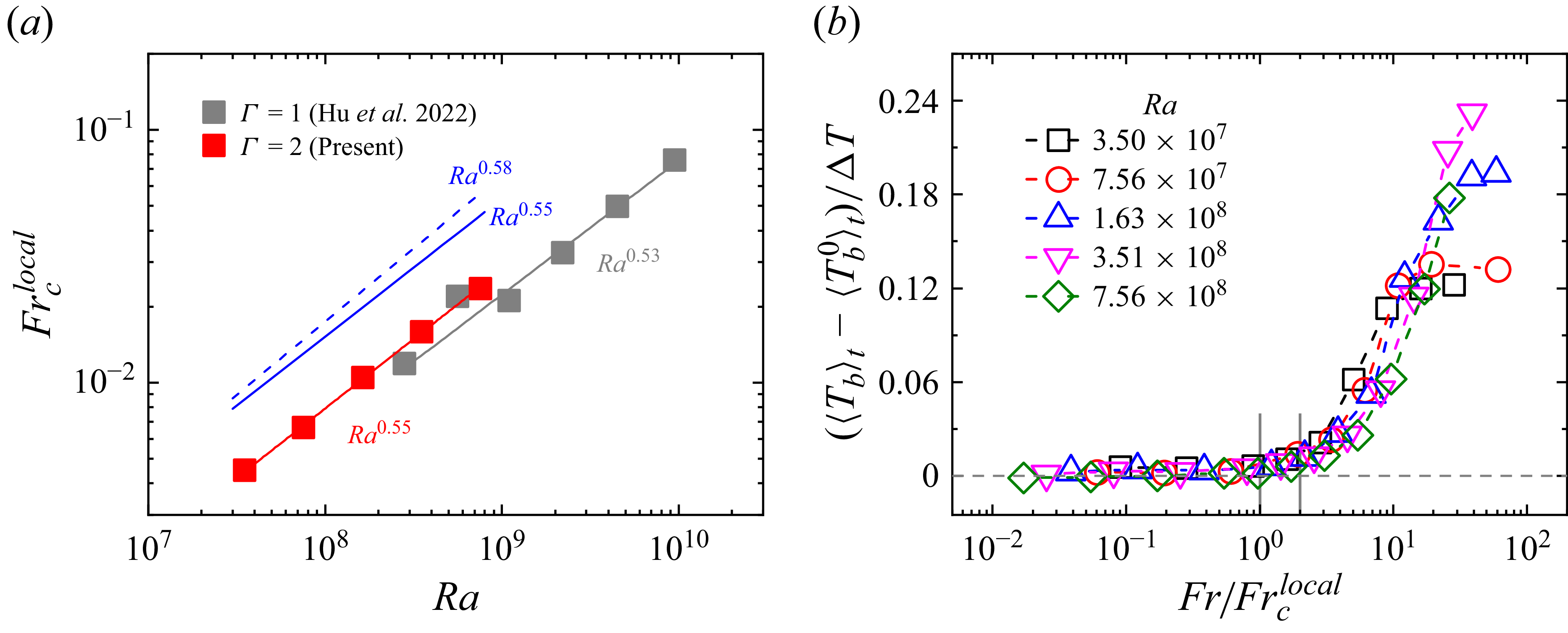
(a) Plots of
 $\textit{Fr}_c^{\textit{local}}$
as a function of
 $Ra$
. The red solid squares in the present study exhibit a power-law behaviour
 $\textit{Fr}_c^{\textit{local}}=3.19\times 10^{-7}Ra^{0.55}$
(the red solid line), which agrees well with previous results (the grey solid squares) with the scaling
 $\textit{Fr}_c^{\textit{local}}=3.79\times 10^{-7}Ra^{0.53}$
(the grey solid line) (Hu et al. Reference Hu, Xie and Xia2022). The blue dashed and solid lines represent the predicted scalings obtained, respectively, from the VAC scales (i.e.
 $\textit{Fr}_c^{\textit{local}}=3.99\times 10^{-7}Ra^{0.58}$
) and the scales from the measured data (i.e.
 $\textit{Fr}_c^{\textit{local}}=6.59\times 10^{-7}Ra^{0.55}$
). (b) The same data as in figure 3(a), but plotted as function of
 $\textit{Fr}/\textit{Fr}_c^{\textit{local}}$
. The dashed line with zero bulk temperature anomaly is the baseline.

4. Understanding the scaling of the onset Froude number
The onset Froude numbers
 $\textit{Fr}_c^{\textit{local}}$
extracted from figure 3(a) are displayed in figure 6(a), which exhibits a power-law scaling
 $\textit{Fr}_c^{\textit{local}}=3.19\times 10^{-7}Ra^{0.55\pm 0.01}$
. Scaling-wise, these results are in good agreement with the experimentally obtained scaling
 $\textit{Fr}_c^{\textit{local}}=3.79\times 10^{-7}Ra^{0.53}$
in a
 $\varGamma =1$
cell (Hu et al. Reference Hu, Xie and Xia2022). After rescaling with
 $\textit{Fr}_c^{\textit{local}}$
, figure 6(b) collapses the bulk temperature anomaly in figure 3(a), indicating that
 $\textit{Fr}_c^{\textit{local}}$
captures the onset behaviour reasonably well. This section is devoted to the understanding of this 0.55 scaling of
 $\textit{Fr}_c^{\textit{local}}$
, based on the local force balance argument proposed by Hu et al. (Reference Hu, Xie and Xia2022).
4.1. The mechanism of local force balance
We first explain the idea of local force balance here, which involves three unknown characteristic scales of vertical velocity
 $U_z$
, length
 $\ell$
and temperature
 $\vartheta$
. The critical Froude number
 $\textit{Fr}_c^{\textit{global}}=R/H$
(Horn & Aurnou Reference Horn and Aurnou2018) was obtained from the balance between the vertical (
 $\tau _{f\!f}$
) and horizontal (
 $\tau _{cb}$
) free-fall time scales, which implicitly assumes free-fall dynamics over global length scales both vertically and horizontally (see § 1). However, this global argument cannot be applied to the cases with strong Coriolis force. On the one hand, due to the strong TP effect, the vertical dynamics is no longer free-fall; on the other hand, the horizontal dynamics becomes diffusive due to the strong interactions between the columnar structures. Therefore, both vertical and horizontal dynamics should be re-examined under strong Coriolis force.
For vertical dynamics at small
 $Ek$
, the vertical time scale of a fluid parcel can be evaluated as
 $\tau _H=H/U_z$
. Since the root mean square (rms) of vertical velocity
 $u_z^{\textit{rms}}=\sqrt {\langle u_z^2\rangle }$
is usually used to evaluate
 $U_z$
(e.g. Abbate & Aurnou Reference Abbate and Aurnou2023), we show, in Appendix A, the normalised rms velocity
 $u_z^{\textit{rms}}/U_{\!f\!\!f}$
measured in the rapidly rotating regime. The small values of
 $u_z^{\textit{rms}}/U_{\!f\!\!f}$
suggest that the vertical dynamics is indeed not free-fall at large rotation speed.
The horizontal dynamics under WC force was investigated by Noto et al. (Reference Noto, Tasaka, Yanagisawa and Murai2019). Similar to the ideal gas system at equilibrium, the mean free distance
 $\ell$
among the columns, and the mean free time
 $\tau _{\ell }$
before one column interacts with another, were introduced. They found that within the mean free distance, a column is accelerated by the WC force until it meets and interacts with another one, resulting in a smaller mean free time compared to that without centrifugal effect. Also, this stop–go motion makes the columns show radial movements with zigzag trajectories. With this physical scenario in mind, one can see that only within the small mean free distance
 $\ell$
can centrifugal buoyancy
 $\alpha (\varOmega ^2R)\vartheta$
affect the horizontal dynamics. Here,
 $\vartheta$
is the typical temperature scale characterising the temperature anomaly of a column. Therefore, the horizontal time scale within which the flow is affected by centrifugal force can be estimated as
 $\tau _{\ell }=\ell /\sqrt {\alpha (\varOmega ^2R)\vartheta \ell }$
.
Now consider a fluid parcel that moves vertically inside a column with
 $U_z$
. It will arrive at, and then be annihilated by, the opposite plate after
 $\tau _H$
. Only if this lifetime
 $\tau _H$
is longer than the mean free time
 $\tau _{\ell }$
can this fluid parcel feel the effect of centrifugal force. Therefore, the critical state is
 $\tau _H\simeq \tau _{\ell }$
, which determines the onset Froude number
 $\textit{Fr}_c^{\textit{local}}$
, i.e.
 \begin{equation} \textit{Fr}_c^{\textit{local}}\simeq \frac {\ell U_z^2}{\alpha g\vartheta\! H^2}=\frac {\ell }{H}\frac {\Delta T}{\vartheta }\!\left(\frac {U_z}{U_{\!\textit{ff}}}\right)^2\!. \end{equation}
4.2. The characteristic scales for
 $\textit{Fr}_c^{\textit{local}}$

The next step is to resolve these three unknown scales in (4.1), namely,
 $\ell /H$
,
 $\vartheta /\Delta T$
and
 $U_z/U_{\!\textit{ff}}$
. Note that working out how these scales behave is also the key issue of the viscous–Archimedean–Coriolis (VAC) and Coriolis–inertial–Archimedean arguments (e.g. Abbate & Aurnou Reference Abbate and Aurnou2023, Reference Abbate and Aurnou2024; Hawkins et al. Reference Hawkins, Cheng, Abbate, Pilegard, Stellmach, Julien and Aurnou2023; Madonia et al. Reference Madonia, Aguirre Guzmán, Clercx and Kunnen2023). For the flow full of columns, Aguirre Guzmán et al. (Reference Aguirre Guzmán, Madonia, Cheng, Ostilla-Mónico, Clercx and Kunnen2021) have shown that the viscous force is important. Therefore, the VAC balance can be applied here to determine these three typical scales.
Briefly speaking, the VAC balance
 $\nu {\nabla} ^2 \boldsymbol{\omega } \sim \boldsymbol{\nabla }\times (\alpha g T \boldsymbol{e}_z) \sim 2\boldsymbol{\varOmega } \boldsymbol{\cdot }\boldsymbol{\nabla }\boldsymbol{u}$
, together with the definition of Nusselt number
 $\textit{Nu} - 1 = \langle u_z \theta \rangle /(\kappa\, \Delta T / H) \sim \textit{Re}_z\,Pr\,\vartheta /\Delta T$
, yields
 \begin{equation} \begin{cases} \ell /H \sim \textit{Ek}^{1/3}, \\ \textit{Re}_z \sim \textit{Ek}^{1/3}\,[Ra\,(Nu-1)]^{1/2}\,\textit{Pr}^{-1}, \\ \vartheta /\Delta T \sim [(Nu-1)/Ra]^{1/2}\,\textit{Ek}^{-1/3}. \end{cases} \end{equation}
Here,
 $\textit{Re}_z$
is the Reynolds number defined as
 $\textit{Re}_z=U_zH/\nu =\sqrt {Ra/Pr}\,U_z/U_{\!f\!\!f}$
. With the measured scaling
 $\textit{Nu}-1=2.5(Ra/Ra_c)^{1.5}$
for present parameters (Sun et al. Reference Sun, Hu, Wang and Xia2024), we finally obtain, from (4.1) and (4.2),
 \begin{equation} \textit{Fr}_c^{\textit{local}}=(2.5/8.7^{1.5})^{0.5}\textit{Pr}^{-1}\textit{Ek}^{7/3}Ra^{5/4}. \end{equation}
It seems that this prediction differs a lot from the experimental result
 $\textit{Fr}_c^{\textit{local}}\sim Ra^{0.55}$
. Let us explain below within the
 $\textit{Fr}{-}Ek$
space.
In principle, the flow state should be kept unchanged (i.e. fix
 $Ra$
and
 $Ek$
) when increasing centrifugal force gradually from zero, waiting for
 $\textit{Fr}$
to exceed
 $\textit{Fr}_c^{\textit{local}}$
. However, in our experiments with a single convection cell, both
 $\textit{Fr}$
and
 $Ek$
are controlled by the rotation rate
 $\varOmega$
; they covary as
 \begin{equation} \textit{Fr}=(R\nu ^2/4gH^4)\,\textit{Ek}^{-2}. \end{equation}
Consequently, the increment of
 $\textit{Fr}$
in the present experiments will be along the path defined by (4.4) in the
 $\textit{Fr}{-}Ek$
space. And the onset Froude number in this situation should be the one obtained by combining (4.3) and (4.4), which gives
 $\textit{Fr}_c^{\textit{local}}=3.99\times 10^{-7}Ra^{0.58}$
. This predicted scaling is displayed in figure 6(a). It can be seen that this 0.58 scaling agrees well with the measured 0.55 scaling, but the magnitude is approximately two times larger. Here, we emphasise that the data in figure 6(b) indicate that it is also reasonably good if the onset Froude number is evaluated as
 $2\textit{Fr}_c^{\textit{local}}$
.
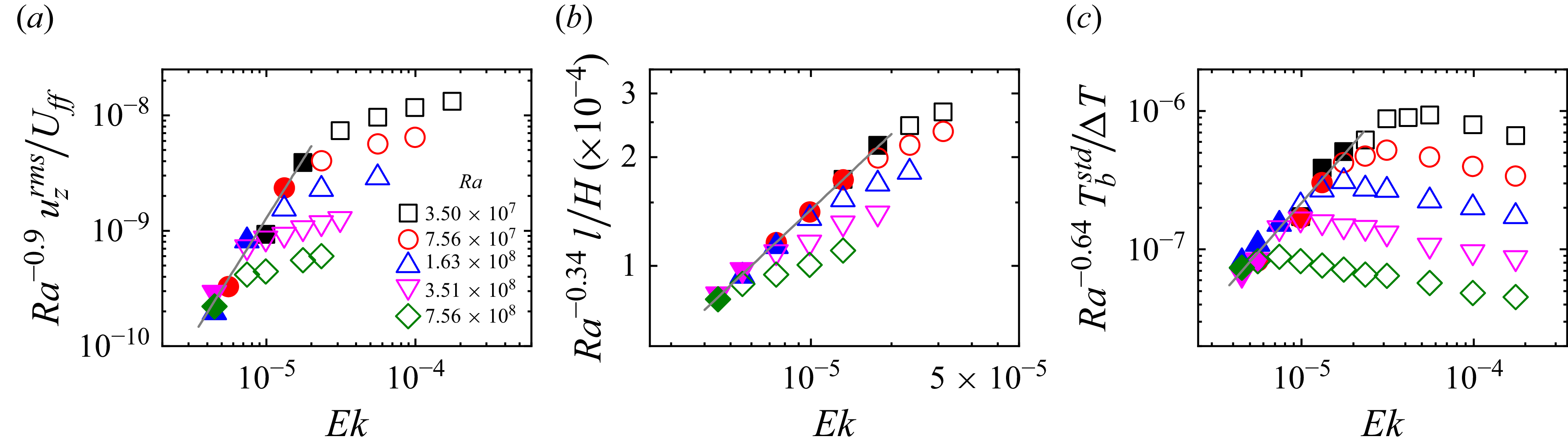
The results in previous studies imply that the VAC scales in (4.2) do not hold exactly (e.g. Abbate & Aurnou Reference Abbate and Aurnou2023, Reference Abbate and Aurnou2024; Hawkins et al. Reference Hawkins, Cheng, Abbate, Pilegard, Stellmach, Julien and Aurnou2023; Madonia et al. Reference Madonia, Aguirre Guzmán, Clercx and Kunnen2023). Therefore, in figure 7, we use our measured data to resolve the corresponding scales. The rms vertical velocities
 $u_z^{\textit{rms}}$
in figure 7(a), calculated from vertical flow fields, are used to evaluate
 $U_z$
(e.g. Abbate & Aurnou Reference Abbate and Aurnou2023). From horizontal flow fields, the column’s effective radius
 $a$
and the centre-distance
 $d$
(i.e. the distance between the centres of two nearby columns) are calculated from the
 $Q$
-fields (refer to our recent paper (Sun et al. Reference Sun, Hu, Wang and Xia2024) for the details). As pointed out by Noto et al. (Reference Noto, Tasaka, Yanagisawa and Murai2019), the column’s real size should be considered when discussing the mean free distance
 $\ell$
. Therefore, the quantity
 $l=d-2a$
is defined to evaluate
 $\ell$
in figure 7(b). It can be seen that for each data set at fixed
 $Ra$
, both
 $u_z^{\textit{rms}}$
and
 $l$
show a transition. As discussed in great detail in Sun et al. (Reference Sun, Hu, Wang and Xia2024), this transition, reflecting the changes of flow structures, is intimately related to the change of heat transfer scaling, signalling the regime transition from CTC to plume regimes. For the present study, only the data in the CTC regime (the solid symbols in figure 7) are utilised to obtain the respective power-law scalings, i.e.
 $u_z^{\textit{rms}}/U_{\!\textit{ff}}=28.2\,Ra^{0.9\pm 0.1}\,\textit{Ek}^{2.1\pm 0.3}$
and
 $l/H=0.43\,Ra^{0.34\pm 0.02}\,\textit{Ek}^{0.70\pm 0.03}$
. The typical temperature scale
 $\vartheta$
can be assessed using the standard deviations of bulk temperature
 $T_b^{\textit{std}}$
(see e.g. Abbate & Aurnou Reference Abbate and Aurnou2023), which is displayed in figure 7(c). Similarly, the data in the CTC regime can be described by a power law
 $T_b^{\textit{std}}/\Delta T=2.8\,Ra^{0.64\pm 0.08}\,\textit{Ek}^{1.4\pm 0.2}$
. Here, all the scaling exponents for
 $Ra$
and
 $Ek$
are obtained by a two-dimensional nonlinear least squares fit (refer to Weiss, Wei & Ahlers Reference Weiss, Wei and Ahlers2016). With these measured scalings, (4.1) can now be written as
 $\textit{Fr}_c^{\textit{local}}=124.3\,Ra^{1.5}\,\textit{Ek}^{3.5}$
. Again, by considering the covarying of
 $\textit{Fr}$
and
 $Ek$
in (4.4), we finally obtain the predicted scaling
 $\textit{Fr}_c^{\textit{local}}=6.59\times 10^{-7}Ra^{0.55}$
. As shown in figure 6(a), this scaling also agrees well with the measured 0.55 scaling.
The compensated plots for (a) the measured rms vertical velocities
 $u_z^{\textit{rms}}$
, (b) the mean free distances
 $l$
, and (c) the bulk temperature fluctuations
 $T_b^{\textit{std}}$
. The data in the CTC regime (the solid symbols) are described by the respective power-law scalings (the grey solid lines), i.e.
 $u_z^{\textit{rms}}/U_{\!\textit{ff}}=28.2\,Ra^{0.9\pm 0.1}\,\textit{Ek}^{2.1\pm 0.3}$
,
 $l/H=0.43\,Ra^{0.34\pm 0.02}\,\textit{Ek}^{0.70\pm 0.03}$
and
 $T_b^{\textit{std}}/\Delta T=2.8\,Ra^{0.64\pm 0.08}\,\textit{Ek}^{1.4\pm 0.2}$
.

The satisfactory predictions from dimensional analysis in (4.2) and experimental data in figure 7 suggest that the underlying mechanism for
 $\textit{Fr}_c^{\textit{local}}$
is well captured by the mechanism of local force balance (i.e. (4.1)).
5. Conclusions
The effects of weak centrifugal (WC) force on bulk and sidewall flows in turbulent rotating Rayleigh–Bénard convection are investigated experimentally in this study. For the bulk flow, PIV measurements reveal a hot cyclonic structure in long-time averaged mean fields, which is consistent with the increased mean bulk temperature measured at cell centre. However, for the instantaneous fields, individual hot and cold columns can still be easily recognised even for
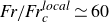 $\textit{Fr}/\textit{Fr}_c^{\textit{local}}\simeq 60$
, as if the centrifugal force were not present. As for the sidewall flow, azimuthal flow fields clearly show that the sidewall region is dominated by the boundary zonal flow (BZF), whose properties, however, exhibit huge differences from reported results. From these findings, together with the decreased sidewall temperature at large
 $\textit{Fr}$
, we presume that the BZF has already been contaminated by the WC force. Unlike the strong centrifugal (SC) effects, the WC effects are much less clear, and are often simply ignored in most experiments. Therefore, the present results can help to ascertain in which situation the WC effects can be safely dropped in experiments.
After identifying how the WC force manifests itself, we then investigate when these effects start to set in, i.e. the onset Froude number
 $\textit{Fr}_c^{\textit{local}}$
. Different from the conventional constant value
 $0.05$
(e.g. Marques et al. Reference Marques, Mercader, Batiste and Lopez2007),
 $\textit{Fr}_c^{\textit{local}}$
is instead found to depend on
 $Ra$
as
 $\textit{Fr}_c^{\textit{local}}\sim Ra^{0.55}$
. Together with our previously measured results (Hu et al. Reference Hu, Xie and Xia2022), this 0.55 scaling covers a wide Rayleigh number range
 $3.5\times 10^7 \leqslant Ra \leqslant 9.3\times 10^9$
, indicating the robustness of this scaling. To reveal the underlying mechanism for this robust scaling, a dimensional analysis based on the mechanism of local force balance is applied. The resulting
 $\textit{Fr}_c^{\textit{local}}$
in (4.1) contains three unknown characteristic scales, which can be resolved either by VAC arguments or by our experimental data. The final predicted scalings of
 $\textit{Fr}_c^{\textit{local}}$
are found to agree excellently with the 0.55 scaling of
 $\textit{Fr}_c^{\textit{local}}$
, indicating that this local-force-balance model correctly describes the flow’s local dynamics, and therefore may help in modelling the WC effects in future study.
In the present study, the details about how the WC force modifies the BZF remain unclear. Also, it can be expected that with increasing
 $\textit{Fr}$
, the BZF will finally be replaced by the cold downwelling flow near the sidewall. It will be interesting to find out how and when this transition occurs. On the other hand, the verification of the predicted
 $\textit{Fr}_c^{\textit{local}}$
scaling may need help from numerical studies, since
 $\textit{Fr}$
and
 $Ek$
can be easily varied independently in simulations. All these unresolved issues need further study.
Funding
This work is supported by the National Natural Science Foundation of China (NSFC) (grant nos 12072144, 12232010). Y.B.H. is also supported by NSFC (grant no. 12402253) and the China Postdoctoral Science Foundation (grant no. 2024M764075).
Declaration of interests
The authors report no conflict of interest.
Appendix A.
The table below shows the parameters and the data collected for different
 $Ra$
. The first four columns are the control parameters. Here, the onset Rayleigh number is
 $Ra_c=(8.70{-}9.63\,\textit{Ek}^{1/6})\,\textit{Ek}^{-4/3}$
. The next three columns are the normalised mean bulk temperatures
 $\langle T_b \rangle _t/ \Delta T$
, the sidewall temperatures
 $\langle T_w \rangle _{\phi ,t} / \Delta T$
and bulk temperature fluctuations
 $T_b^{\textit{std}}/ \Delta T$
, respectively. The remaining columns are the quantities from the PIV measurements: the normalised width of BZF
 $\delta _0 / R$
, the width of velocity layer
 $\delta _{\textit{max}} / R$
, the rms values of vertical velocity
 $u_z^{\textit{rms}}/ U_{ff}$
, the radius of columns
 $a/H$
, and the centre-distance
 $d/H$
.