1. Introduction
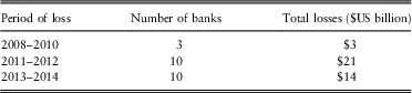
Li et al. (Reference Li, Allan and Evans2017) analysed extreme operational risk events in US and EU banks from 2008 to 2014Footnote 1 based on data provided by ORIC International, where an extreme event was one where the recorded loss was greater than $US100 million. The number and amount of the extreme operational risk losses determined by Li et al. (Reference Li, Allan and Evans2017) are summarised in Table 1.
Extreme operational risk losses.

Over the period 2008–2014, US banks incurred almost $700 billion losses from extreme operational risk events, and EU banks incurred almost $200 billion losses. In terms of relative impact, losses over $1 billion clearly have the greatest impact on profits and extreme operational risk losses in banks appear highly skewed which is consistent with the results in Ganegoda & Evans (Reference Ganegoda and Evans2013). Just to put these losses into perspective, the total assets of US and EU banks at the end of 2014 were $US 16 trillionFootnote 2 and $US 23 trillionFootnote 3 , respectively, spread across 5,573 US banks and 3,972 EU banking groups. Whilst the number of banks incurring the extreme operational risk events is then relatively small and the impact on the banks’ asset bases is moderate, there is a much greater impact on the share price and hence the reputation of the offending banks. Sturm (Reference Sturm2013) considered the impact on German banks’ share price of announcements of operational losses and concluded that there was evidence of negative cumulative abnormal returns following both the announcement of the operational loss and the announcement of the settlement. Similarly, Fiordelisi et al. (Reference Fiordelisi, Soana and Schwizer2014) concluded from a study of operational risk losses in US and EU banks between 1994 and 2008 that there was substantial reputational damage following the announcement of the losses. Given the likely disproportionate impact on each bank when an extreme operational risk event occurs, it may well be in the interests of banks to develop a pooling or insurance arrangement for these larger losses to reduce the impact on share price of the individual bank. Such a pooling arrangement may well be of interest to regulators as significant reputational damage to a bank may affect the stability of the banking system. In this paper, we will only consider the feasibility of an inter-bank pooling arrangement, but we recognise that insurers may well be able to offer insurance even if an inter-bank pooling arrangement were not feasible if they have other uncorrelated insured risks. This paper is concerned only with the actuarial issues around the feasibility of an extreme operational risk pooling arrangement and not with the other issues such as regulatory and political feasibility.
2. Sustainable Pooling Issues
The main actuarial criteria for a sustainable pooling arrangement for extreme operational risk events is that the expected frequency and severity of claims must be reasonably predictable within acceptable bounds. To achieve this the pool needs a sufficiently large number of participants with identifiable and bounded potential losses and where the different risks are priced appropriately. In addition, the feasibility of the pooled arrangement would be greatly enhanced if there could be shown there was a low expected correlation of events across the banks, as this would allow a pricing structure that would be advantageous to participating banks as their contribution to the pool would be less than the losses potentially incurred by themselves. The pooled arrangement would then allow a spreading of costs across banks and across time. In this paper, given the low frequency of observed extreme operational risk events, and the actuarial importance of the correlation of extreme operational risk events to the feasibility of the pool concept, we will use two approaches to analyse the historical occurrence of extreme operational risk events:
∙ First, we will determine the Pearson coefficient for losses versus year of occurrence and bank name versus year of occurrence to determine statistically the independence of the extreme operational risk events. As the number of events being considered is relatively small, we will also observe the number of banks with single-year events and multiple-year events as a proxy for the frequency of events and observe for those with single events, the distribution of the events across the years as a proxy for correlation.
∙ Second, given the relatively small number of extreme operational risk events that can be quantitatively assessed with any reliability for determining future occurrences, we will use a qualitative assessment and consider the underlying characteristics of the historical extreme operational risk events to determine the drivers of the events as a means of understanding the commonality of the drivers and hence the likely correlation of future events.
3. Empirical Analysis
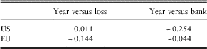
Table 2 shows the Pearson Coefficient for US and EU extreme operational risk losses against the year of loss, and also the year of loss against the bank name which was determined by giving each bank a unique numerical code.
Pearson coefficient.

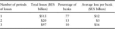
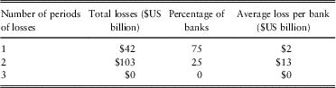
The Pearson coefficient indicates there is no significant correlation between losses and years, nor between years and banks, indicating that for the period analysed, losses are reasonably independent within the constraints of the measure used and the relatively small data used. To test the reliability of the Pearson coefficients, the data were categorised into three periods, 2008–2010, 2011–2012 and 2013–2014. Tables 3 and 4 show the distribution of the number of banks incurring multiple period losses, and the average loss.
US banks, distribution of multiple events.

EU banks, distribution of multiple events.

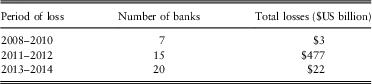
We have also analysed the distribution of single events across the three periods in Tables 5 and 6.
US banks, distribution of single events.

EU banks, distribution of single events.

The results in Tables 3–6 empirically support the implication of the Pearson coefficient and indicate that during the period 2008–2014, around 75% of banks in the United States and the European with extreme operational risk losses had a loss in only 1 period, i.e., most of the banks are not “serial offenders”. In the United States, most of the losses by value have occurred in banks with losses in only one period, but this pattern is not observed in the European where those banks with events in two periods have the most losses by valueFootnote 4 . The US banks with events in all three periods have larger average losses than the other US banks and in the EU banks, those with events in two periods have higher average losses than those banks with only one event. Overall, this analysis suggests that the distribution of losses is heavy tailed with a few banks having both a higher frequency of events and a higher severity of losses. The results in Tables 5 and 6 indicate that by number of banks, there has been a reasonably even distribution of events across the different periods, but the distribution by value of the losses is highly concentrated.
4. Qualitative Analysis
Financial markets, and financial institutions exhibit the features of a complex adaptive system which do not lend themselves to statistical modelling (Daníelsson, Reference Daníelsson2008). Further, Mittnik et al. (Reference Mittnik, Paterlini and Yener2013) counselled against placing too much reliability on both Pearson coefficients and copulas when analysing operational risk co-variability. To give greater breadth and depth to the analysis of the feasibility of a pooled arrangement for sharing extreme operational risk losses across banks, particularly given the relatively small amount of data and the skewness of the extreme operational risk losses, we have determined the drivers of the extreme operational risk events, using a process known as cladistics analysis. This analysis tests for systemic drivers that would suggest high correlation of extreme operational risk events. Cladistics analysis was originally developed to assist biologists to estimate the likely evolutionary path of animals based on their characteristics, but it has recently been more widely used to understand how organisations work (Mitleton-Kelly, Reference Mitleton-Kelly2003), and how cultural inheritance in social systems occurs (Matthews et al., Reference Matthews, Edmonds, Wildman and Nunn2013). In the financial field, cladistics analysis has been used to study the drivers of significant derivative events (Allan & Corrigan, Reference Allan and Corrigan2013), operational risks in banks (Li et al., Reference Li, Allan and Evans2017) and the World Economic Forum 2014 risks (Evans et al., Reference Evans, Allan and Cantle2017). Cladistics analysis produces a hierarchical structure of the characteristics starting from the characteristic that is unique to an event and moving through the characteristics that are common to several events until it determines the characteristic common to the most events that is possible. To construct cladistics trees, we used the maximum parsimony method, which is based on the theorem of Occam’s razor which states that assumptions for explaining phenomenon should be as few as possible so as to construct the tree that minimises the number of steps required to generate the variation in the sequences from the common ancestor. Defining the difference between two sequences with length L,u=(u 1, … , u L ) and v=(v 1, … , v n ), then the non-normalised Hamming distance:
 $$diff\left( {u,v} \right){\equals}\left| {\left\{ {k\,\mid\,u_{k} \,\ne\,v_{k} } \right\}} \right|$$
and given sequences A of length L, with a corresponding tree T, the Parsimony Score is
 $${\rm PS}\left( {T,A} \right){\equals}{\rm }\mathop{{\min }}\limits_{\lambda } \mathop {\sum\limits_{\left\{ {u,v} \right\} \in E}}} diff(u,v)$$
Where the minimum is taken over all possible labels λ of the internal nodes of tree T.
To find the most parsimonious tree, denote the value of the character for node v by c(v), and for each leaf v:
 $$S\left( v \right){\equals}c(v)$$
For inner node v with “children” u, w:
 $$S\left( v \right){\equals}{\rm }\left\{ {\matrix{ {S\left( u \right){\cap}S\left( w \right), \quad S(u){\cap}S(w)\,\ne\,\phi} \cr {S\left( u \right){\cup}S\left( w \right), \quad S(u){\cup}S(w){\equals}\phi} } \right$$
If
 $S(u){\cup}S(w){\equals}\phi$
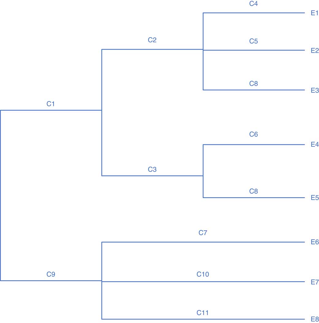
, the parsimony score will be incremented by 1. By enumerating all possible trees, the one with minimum Parsimony Score is the most parsimonious tree. The output of a cladistics analysis is typically a tree structure that makes it easy to see the linkages that are estimated to have occurred. Figure 1 shows a simple illustrative cladistics tree for a series of events E1–E8, and their characteristics C1–C11. In this simple system, Event 1 has characteristics C1, C2 and C4 and shares C2 with Events 2 and 3, and C1 with Events 2, 3, 4 and 5. C1 and C9 can be regarded as the most systemic characteristics, i.e., they are the most common characteristics, whilst C4, C5, C6 and C8 are the least systemic. Real systems usually are a lot more complex than shown in Figure 1 with several branches between the systemic and least systemic or unique characteristics. Characteristics C1 and C9 can be thought of as the “Tier 1” characteristics, and C2, C3, C7, C10 and C11 as the “Tier 2” characteristics. In an analysis of financial systems, the input is a list of events with their characteristics derived from descriptions of the events either simply from observation or analysis of the common words used in the description of the event, with the consistency index used to give comfort that the characteristics chosen give a consistent output.
A typical cladistics tree.

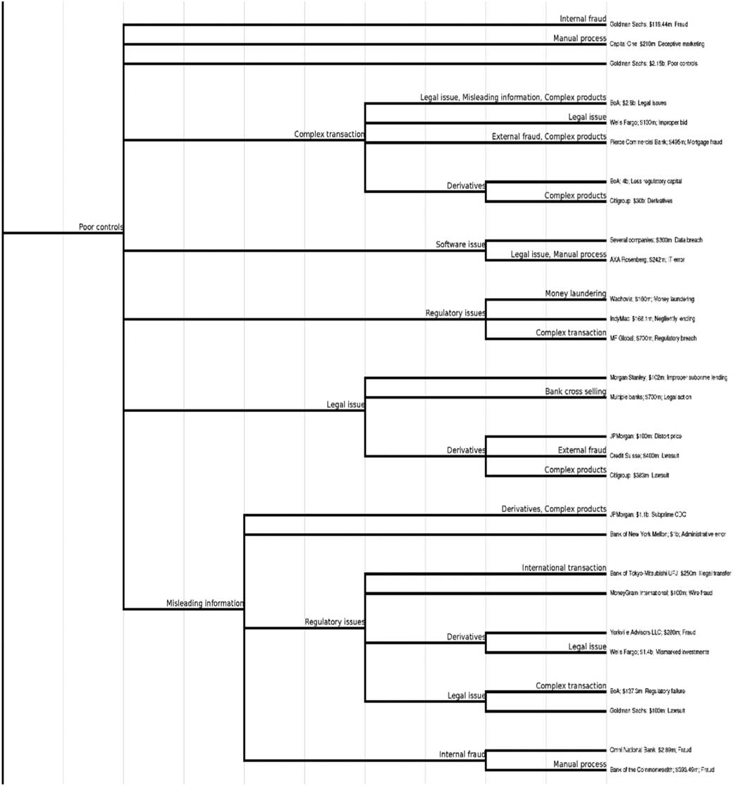
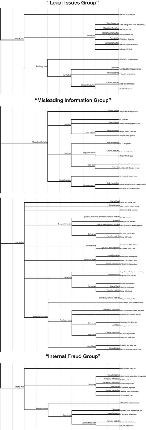
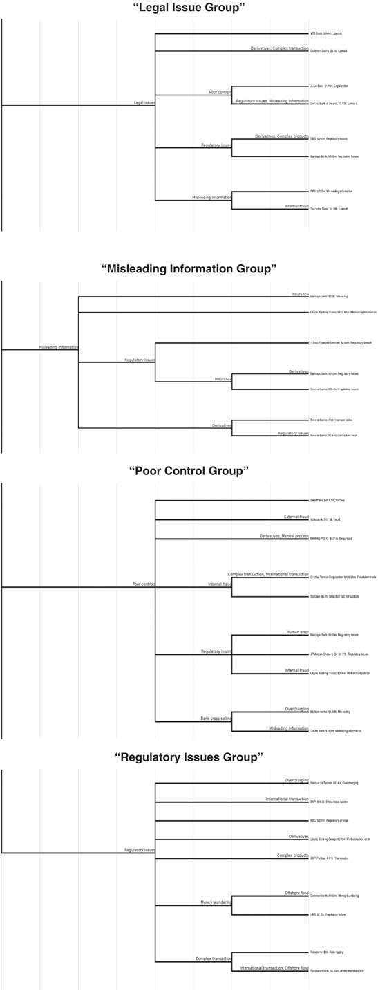
We have used cladistics analysis to determine the systemic drivers of the US and EU extreme operational risk events over the period 2008–2014. A high degree of commonality and sustainability of the systemic drivers of the extreme operational risk events across banks and across geographic zones would be indicative that in the longer term, banks may well have similar events with a high correlation of losses as the events are driven by common characteristics. The cladistic trees for US and EU extreme operational risk losses over the period 2008–2014 are shown in Appendix A for the more significant groupsFootnote 5 . A sample “tree” for the “US poor controls group” is shown in Figure 2.
US poor controls group.

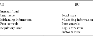
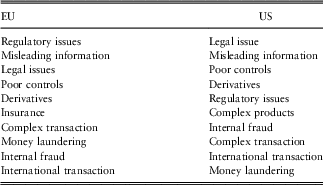
The most systemic characteristics, i.e., those on the left side of the trees are summarised in Table 7.

The results in Table 7 indicate that there is significant commonality in the systemic characteristics of the extreme operational risk events across the US and the EU banks. Furthermore, the number of systemic characteristics is reasonably small, indicating a significant commonality in the major drivers of extreme risk events. This result is consistent with the findings of Chernobai et al. (Reference Chernobai, Jorion and Yu2011) who found what we have called poor controls was also a significant driver of operational risk events but our study questions the assumption Chernobai et al. (Reference Chernobai, Jorion and Yu2011) made of independence of operational risk events, and also questions the reliability of quantitative analysis, such as the Pearson coefficient when analysing extreme events in a complex adaptive system. The cladistics analysis has a similar objective to that of Chavez-Demoulin et al. (Reference Chavez-Demoulin, Embrechts and Hofert2016) who analysed covariates of causes of operational risk events, but our analysis uses a different approach and importantly, does not make any assumption as to independence of the risk events and has shown there is significant dependence in terms of the systemic characteristics of extreme operational risk events.
5. Network Analysis
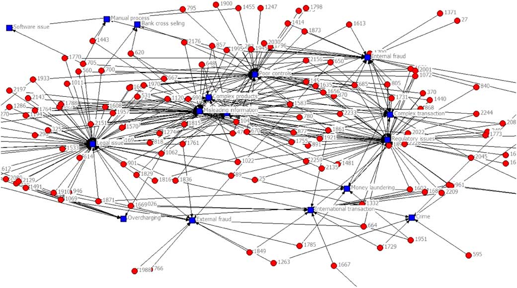
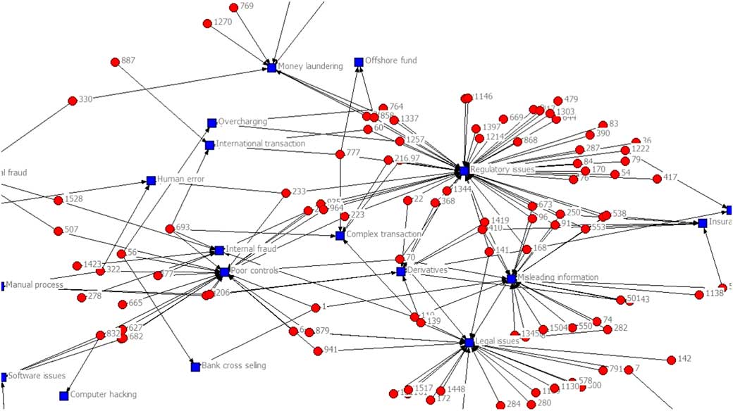
Cladistics analysis identifies the systemic characteristics of risk events, but a closer observation of the trees in Appendix A will show that the systemic characteristic for a particular group of events also occurs in other groups of events at lower levels of systemic importance. It is difficult to easily identify the overall extent of the influence of some characteristics from the cladistics analysis where the characteristics occur in several groups of events. Network analysis is concerned with the totality of the influence of characteristics on the risk events and compliments the cladistics analysis. Network analysis of the financial system is gaining attention with recent papers including Haldane & May (Reference Haldane and May2011) who looked at the systemic risk in the banking system resulting from interconnectedness, Battiston et al. (Reference Battiston, Farmer, Flache, Garlaschelli, Haldane, Heesterbeek and Scheffer2016) who argued economic policy needs interdisciplinary network analysis and behavioural modelling and Joseph & Chen (Reference Joseph and Chen2014) who looked at interconnectedness indicators as predictors of potential financial crises. We will use network analysis to indicate the overall degree of importance in the network of the characteristics of extreme operational risk losses. Based on Bavelas (Reference Bavelas1950) and Leavitt (Reference Leavitt1951) and the features of the network, we have used eigenvector centrality as the measure of importance of the characteristics. Figures 3 and 4 set out the network diagrams for the US and EU extreme operational risk events and their characteristics with the major connectivityFootnote 6 . The red dots are the extreme operational risk events and the blue squares are the dominant characteristics that are linked to the risk events. The more graphically central the characteristic, the more events are connected to it.
US major connections.

EU major connections.

The dominant characteristics from Figures 3 and 4 are summarised in Table 8 in descending order of degrees of connectivity which measures the number of risk events connected to each characteristic.
Dominant network characteristics for operational risk events 2008–2014.

The results in Tables 7 and 8 indicate that there is not much difference between the dominant characteristics determined by the cladistics analysis and the network analysis, but the network analysis has found that there are more common characteristics between the US and EU banks than appears from the cladistics analysis. The combined result is indicative of there being significant commonality of the systemic characteristics of extreme operational risk events across the United States and the European, but the network analysis indicates there is a reasonable range of causes of the extreme operational risk events.
6. Feasibility of an Extreme Operational Risk Pool
In order for a pooled arrangement for sharing extreme operational risk losses across banks to be actuarially sustainable, it is necessary that there are a large number of participants, the expected losses are reasonably determinable, and to be economically attractive, correlations of these extreme operational risk events between the participants should be low. Our analysis shows:
∙ The EU and US banking systems do have a large number of potential participants.
∙ The number of banks with extreme operational risk events is relatively small, and the losses are highly skewed, indicating that statistically based pricing may be difficult.
∙ The banks with extreme operational risk events do not appear to be serial offenders, i.e., the losses appear to be reasonably spread over the banks that have these losses, and by implication, extreme operational risk events could occur for all banks.
∙ There are a small number of systemic characteristics or drivers of the extreme operational risk events, but these main drivers occur also as lower level characteristics in other risk events, and the overall number of significant drivers is reasonably large.
These features of extreme operational risk events would suggest that it might be difficult to convince a large number of banks who have not incurred these extreme losses to join a pooled arrangement, and for the pool to be feasible, regulatory compulsion may be required “in the interests of the economy” to achieve stability of the banking system. On the positive side, the lack of serial offenders, and the reasonably large number of significant characteristics would suggest that sufficient diversification within the pool may be achievable, but this is derived from the reasonably large number of drivers of the extreme events and not from international diversification, so country-specific pooled arrangements could be feasible, at least in the United States and European. Pricing of the risks involved would require capping the losses claimable due to the highly skewed distribution of losses and the potential for unexpected losses.
7. Potential Pooled Arrangements
The analysis suggests that for at least the US and EU banks, pooled arrangements could be established domestically, but smaller economies may need to establish pools across several economies simply to have adequate numbers of participants. But even in the United States and European, compulsory participation and capping of losses that could be claimed would be required to make the pool economically attractive. Given the results of Ganegoda & Evans (Reference Ganegoda and Evans2013), a charging structure based on each bank’s assets would appear reasonable and simple to operate.
8. Conclusion
A pooled arrangement to insure EU and US banks would appear feasible and would be justified in terms of the benefits to shareholders from avoiding severe share price declines when extreme operational risk events are announced and settled, and the advantage to the community of reducing the risk of instability in the banking system.