1 Introduction
The effect of wall texture on fluid motion is a long-standing research topic of both fundamental and practical interest in a variety of fields. A particularly important class of hydrodynamics problems concerns the role of random surface topography (Darcy Reference Darcy1857; Moody Reference Moody1944; Nikuradse Reference Nikuradse1950; Richardson Reference Richardson1973; Kandlikar, Joshi & Tian Reference Kandlikar, Joshi and Tian2003; Hao et al. Reference Hao, Yao, He and Zhu2006; Kunert & Harting Reference Kunert and Harting2007; Vinogradova & Belyaev Reference Vinogradova and Belyaev2011; Zayernouri et al. Reference Zayernouri, Park, Tartakovsky and Karniadakis2013; Yan et al. Reference Yan, Zhang, Peng and Meng2015; MacDonald et al. Reference MacDonald, Chung, Hutchins, Chan, Ooi and García-Mayoral2017). Given sufficient spatial resolution, virtually any natural or manufactured surface exhibits irregular fluctuations of shape. There is a need to understand how the inevitable imperfectness affects the performance of fluidic devices and flow properties in natural systems. This is particularly relevant to the low-Reynolds-number flows typical in nano/microfluidic and chemical microprocess applications where the small length scales of devices imply significant boundary effects (Taylor, Carrano & Kandlikar Reference Taylor, Carrano and Kandlikar2006; Chen et al. Reference Chen, Zhang, Shi and Peterson2009). One of the challenges here is that the statistical properties of the random surface roughness may be poorly specified or completely unknown a priori. Depending on the processing methods and material properties, the resulting roughness of the manufactured surface may be Gaussian or non-Gaussian in height distribution, exponential or non-exponential in the decay of spatial correlations, isotropic or anisotropic, etc. Given such a diversity of alternatives, the issue of universality comes to the fore. Can we formulate any general conclusions concerning the influence of random roughness on fluid motion that hold true regardless of the fine details of the roughness statistics?
Here we implement a perturbative method together with statistical tools to address this question for the low-Reynolds-number flow of an incompressible Newtonian fluid bounded by a no-slip rough wall. Clearly, any deviation of the boundary from an ideal geometrical shape produces a perturbation of the fluid velocity field anticipated in the idealized case. For steady fluid motion in the spatial domain with a stochastically rough boundary, the resulting perturbation is stationary in time but fluctuates in space. Our analysis is focused on the statistical properties of these roughness-induced fluctuations in the ‘wavy’ limit, when the characteristic height
 $h$
of the surface imperfections is much smaller than their characteristic transverse size,
 $l\gg h$
.
Various materials (polymers, glass, metals, ceramics) and a number of processing methods (micromilling, etching, injection moulding, laser micromachining, photolithography, etc.) are used in the fabrication of microchannels – see Prakash & Kumar (Reference Prakash and Kumar2015) and Gale et al. (Reference Gale, Jafek, Lambert, Goenner, Moghimifam, Nze and Kamarapu2018) for recent reviews. An examination of the available experimental data on the spatial scales of surface roughness indicates that in many cases the assumption
 $l\gg h$
is quite reasonable. For example, for the etching process, typical values for the correlation length range between
 $2~\unicode[STIX]{x03BC}\text{m}$
and
 $12~\unicode[STIX]{x03BC}\text{m}$
, while the typical (root-mean square, r.m.s.) roughness amplitude is from 10 nm to 100 nm (see Ren, Ganapathysubramanian & Sundararajan Reference Ren, Ganapathysubramanian and Sundararajan2011; Jaeger et al.
Reference Jaeger, Ren, Xie, Sundararajan, Olsen and Ganapathysubramanian2012; Ren & Sundararajan Reference Ren and Sundararajan2012). The high-precision mechanical processing methods typically produce surfaces with
 $h$
of the order of several micrometres or smaller, while
 $l$
is of the order of tens of micrometres (Bigerelle, Gautier & Iost Reference Bigerelle, Gautier and Iost2007; Zhou et al.
Reference Zhou, Chen, Wang and Jiang2017). Depending on the light wavelength and material properties, the widely used laser processing accompanied by postprocess smoothing typically results in a surface roughness amplitude below several micrometres and a correlation length of one order of magnitude larger (Wang et al.
Reference Wang, Zheng, Lim, Wang and Lam2011; Abdo et al.
Reference Abdo, El-Tamimi, Anwar, Umer, Alahmari and Ghaleb2018). At the same time, some fabrication approaches (e.g. microinjection moulding; see Jia et al.
Reference Jia, Song, Liu and Wang2018) may produce roughness with amplitude comparable to the correlation length; in these cases, the theoretical analysis presented below can provide only a qualitative insight into the effect of surface roughness on the fluid motion. Note also that some material processing methods give rise to a rather regular anisotropic pattern of surface asperities (Young, Brackbill & Kandlikar Reference Young, Brackbill and Kandlikar2009; Grzesik, Rech & Żak Reference Grzesik, Rech and Żak2015). Although the theoretical approach applied below allows one to incorporate the effect of a regular roughness component in a straightforward manner, the main focus of this article is on the case of essentially stochastic roughness.
Let us briefly overview the structure and the main results of this paper. Starting with the simplest setting, namely, the two- (2D) and three-dimensional (3D) flows in a half-space over a flat rough wall, we characterize the fluid velocity fluctuations in terms of their spatial intensity profile, one-point probability distribution, pair correlation function and energy spectrum. At distances
 $z\gg l$
from the wall, these objects are found to exhibit universal behaviour insensitive to the fine details of the roughness statistics. In particular, the far-field velocity fluctuations are Gaussian and their intensity as a function of distance from the wall demonstrates the power-law scaling. Although the properties of the velocity fluctuations in the region
 $z\lesssim l$
are non-universal, it turns out that different surfaces produce flow patterns with common qualitative features.
Next, motivated by recent experiments and simulations by Jaeger et al. (Reference Jaeger, Ren, Xie, Sundararajan, Olsen and Ganapathysubramanian2012), we consider 2D and 3D fluid flows in a plane channel between two parallel walls, one of which is rough, while the other is perfectly flat. The distance
 $d$
between the walls of the channel is assumed to be much larger than the characteristic height
 $h\ll d$
of the surface imperfections. If the correlation length
 $l$
is much shorter than the distance
 $d$
between the walls, the statistical properties of the velocity fluctuations in the channel are universal. Otherwise, when the correlation length
 $l$
is comparable with or larger than
 $d$
, the results are not universal, but again we pay special attention to common qualitative features of the produced fluid flows. The main difference between the fluid flow in a channel and in the half-space over a rough wall is that the large-scale velocity fluctuations are suppressed inside the channel. This is demonstrated by analysis of the energy spectrum of velocity fluctuations as a function of the distance to the rough wall in these two cases.
Finally, we study how the roughness-induced fluctuations in the stationary fluid flow affect the mass transport in the wall-normal direction. Being advected by the mean flow, the passive tracers are subject to the relatively weak flow disturbances generated by the rough wall. At sufficiently large time scale, one may expect to see the spatial dispersion of tracers due to these random disturbances. We show, however, that the spatial dispersion in the wall-normal direction quickly reaches some value and no longer changes with time/distance (along the channel). Therefore, the small-amplitude roughness of the channel walls does not lead to the enhancement of mixing.
2 Model formulation
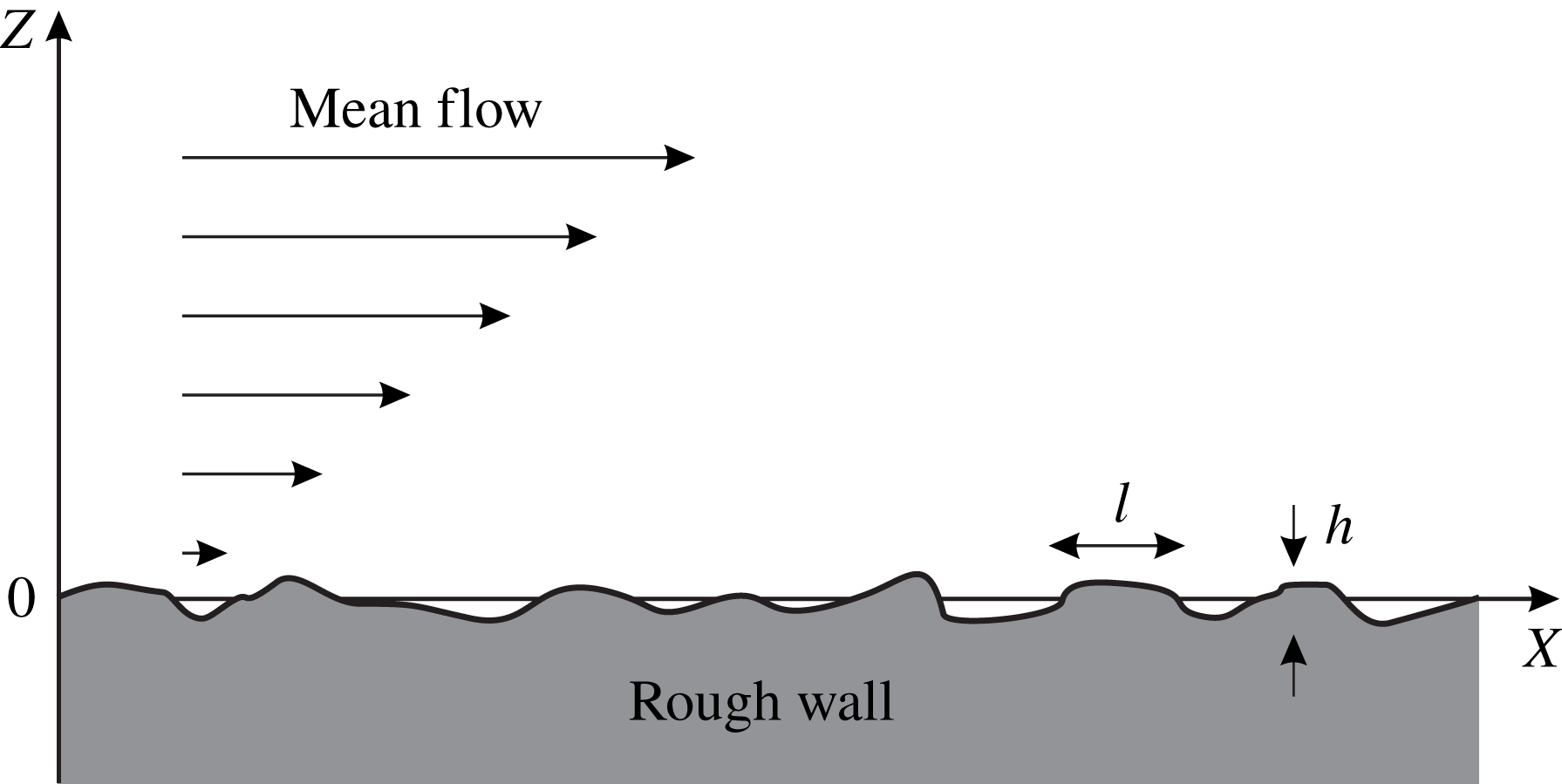
Let us consider the steady fluid flow in a half-space bounded by a wall which is flat on average but has random surface imperfections (see figure 1). The
 $X$
-axis of the Cartesian coordinates is directed along the mean flow, while the
 $Z$
-axis is perpendicular to the wall. To illustrate the main ideas, first we use the 2D model, where wall texture is translationally invariant in the spanwise direction. The generalization to the 3D case will be discussed in § 8. In the 2D model the deviation of the wall surface from the average level
 $z=0$
can be described as
 $$\begin{eqnarray}z=\unicode[STIX]{x1D709}(x),\end{eqnarray}$$
where
 $\unicode[STIX]{x1D709}(x)$
is a single-valued function of the streamwise coordinate.
Within the statistical framework, the roughness amplitude
 $\unicode[STIX]{x1D709}(x)$
is characterized by the surface height distribution
 $P(\unicode[STIX]{x1D709})=\langle \unicode[STIX]{x1D6FF}(\unicode[STIX]{x1D709}-\unicode[STIX]{x1D709}(x))\rangle$
, and the spatial coherence of the surface profile is described by the pair correlation function
 $F(r)=\langle \unicode[STIX]{x1D709}(x)\unicode[STIX]{x1D709}(x+r)\rangle$
. Here the angle brackets mean the coarse-graining averaging over a scale that is much larger than the correlation length
 $l$
of surface imperfections, but much smaller than the size of the system. We also imply homogeneity of the roughness statistics so that the height distribution
 $P(\unicode[STIX]{x1D709})$
is the same at any point of the wall and the pair correlation function
 $F(r)$
is a function of inter-point distance
 $r$
and does not depend on the
 $x$
-coordinate. Note that the function
 $F(r)$
is even in
 $r$
.
While in most theoretical studies the surface height distribution is assumed to be Gaussian, experimental data indicate that real surfaces quite often exhibit non-Gaussian fluctuations in shape (Ren et al.
Reference Ren, Ganapathysubramanian and Sundararajan2011). As for the pair correlation function of
 $\unicode[STIX]{x1D709}(x)$
, it is believed to be well approximated by an exponential function for most fabrication techniques (Bhushan Reference Bhushan2001; Ren et al.
Reference Ren, Ganapathysubramanian and Sundararajan2011). Being interested in model-independent features, here we do not specify the form of functions
 $P(\unicode[STIX]{x1D709})$
and
 $F(r)$
, assuming only that the surface height distribution
 $P(\unicode[STIX]{x1D709})$
has zero mean and finite variance, and the characteristic height of the surface imperfections
 $h$
is much smaller than their correlation length,
 $l\gg h$
. The first assumption ensures that the surface asperities have well-defined characteristic amplitude
 $h$
, while the second assumption means that we deal with a slowly varying boundary, whose effect on the fluid motion can be analysed within the perturbative approach (Van Dyke Reference Van Dyke1964); see § 3.
Viscous fluid flow over a no-slip rough wall, which is flat on average but has random surface imperfections.

When the Reynolds number is very small, the Stokes approximation is adequate in describing the fluid motion (Landau & Lifshitz Reference Landau and Lifshitz1987). The Stokes flow of an incompressible fluid is described by the equations
 $$\begin{eqnarray}\unicode[STIX]{x1D702}\unicode[STIX]{x1D6FB}^{2}\boldsymbol{v}=\unicode[STIX]{x1D735}p,\quad \unicode[STIX]{x1D735}\boldsymbol{\cdot }\boldsymbol{v}=0,\end{eqnarray}$$
where
 $\boldsymbol{v}$
is the 2D flow velocity,
 $p$
is pressure and
 $\unicode[STIX]{x1D702}$
is the dynamic viscosity coefficient. Note that
 $\unicode[STIX]{x1D6FB}^{2}p=0$
, as a consequence of (2.2). Next, we need to impose the no-slip boundary condition at the surface of the wall,
 $$\begin{eqnarray}\boldsymbol{v}|_{z=\unicode[STIX]{x1D709}(x)}=0,\end{eqnarray}$$
which implies that there is no effective slip due to, for example, micro-sized air bubbles (Vinogradova & Belyaev Reference Vinogradova and Belyaev2011). Also, the Knudsen number calculated on the typical roughness element must be small to justify the continuum assumption and, thus, the applicability of the Stokes equation.
3 Perturbative approach
In general, the fluid velocity field can be represented as
 $$\begin{eqnarray}\boldsymbol{v}=\boldsymbol{U}+\boldsymbol{u},\end{eqnarray}$$
where
 $\boldsymbol{U}$
is the velocity in the problem with perfectly flat wall and
 $\boldsymbol{u}$
is the roughness-induced correction. Assuming that
 $\unicode[STIX]{x1D709}(x)=0$
, we readily obtain from (2.2) and (2.3) the shear velocity profile
 $U_{x}=sz$
, where
 $s$
is the shear rate. If the surface imperfections have characteristic height
 $h$
and transverse size
 $l\gg h$
, then in analysing the flow pattern in the region
 $z\gg h$
one can treat
 $\boldsymbol{u}$
as a relatively small perturbation to
 $\boldsymbol{U}$
obeying the following boundary value problem:
 $$\begin{eqnarray}\displaystyle \unicode[STIX]{x1D702}\unicode[STIX]{x1D6FB}^{2}\boldsymbol{u}=\unicode[STIX]{x1D735}p,\quad \unicode[STIX]{x1D735}\boldsymbol{\cdot }\boldsymbol{u}=0, & & \displaystyle\end{eqnarray}$$
 $$\begin{eqnarray}\displaystyle u_{x}|_{z=0}=-s\unicode[STIX]{x1D709}(x),\quad u_{z}|_{z=0}=0,\quad \boldsymbol{u}|_{z\rightarrow \infty }\rightarrow 0. & & \displaystyle\end{eqnarray}$$
Equation (3.3) was obtained from the exact boundary condition (2.3) by expanding the velocity field
 $\boldsymbol{v}$
near
 $z=0$
in a Taylor series. The condition
 $l\gg h$
of a small amplitude of roughness allows us to neglect all the other terms of this Taylor series. The approach fails when
 $h$
becomes comparable with
 $l$
.
The presented boundary perturbation method is well known in fluid mechanics (Van Dyke Reference Van Dyke1964) and has been widely used to analyse the effect of small-amplitude boundary roughness on fluid motion (see e.g. Lessen & Huang Reference Lessen and Huang1976; Wang Reference Wang1976, Reference Wang1978, Reference Wang1979; Phan-Thien Reference Phan-Thien1980, Reference Phan-Thien1981a ,Reference Phan-Thien b ; Pozrikidis Reference Pozrikidis1987; Wang, Wang & Zhang Reference Wang, Wang and Zhang2005; Wang Reference Wang2006). Note, however, that in the majority of these studies the roughness is considered to be regular: the surface profile is described by a single harmonic function or by a superposition of several harmonics. The only exception to this trend is a series of publications by Phan-Thien (Reference Phan-Thien1980, Reference Phan-Thien1981a ,Reference Phan-Thien b ), where the Stokes flow rate enhancement as a function of the statistics of the corrugation is analysed. To the best of our knowledge, our work is the first attempt to combine a perturbative approach with the statistical tools to make analytical predictions concerning the statistics of flow fluctuations generated by stochastic roughness.
Owing to the incompressibility condition (3.2), the velocity field
 $\boldsymbol{u}=(u_{x},u_{z})$
can be written in terms of the streamfunction
 $\unicode[STIX]{x1D713}(x,z)$
:
 $$\begin{eqnarray}u_{x}=\unicode[STIX]{x2202}_{z}\unicode[STIX]{x1D713},\quad u_{z}=-\unicode[STIX]{x2202}_{x}\unicode[STIX]{x1D713}.\end{eqnarray}$$
By substituting these expressions into the boundary value problem (3.2)–(3.3), we find that the streamfunction satisfies the biharmonic equation
 $$\begin{eqnarray}\unicode[STIX]{x1D6FB}^{4}\unicode[STIX]{x1D713}(x,z)=\frac{\unicode[STIX]{x2202}^{4}\unicode[STIX]{x1D713}}{\unicode[STIX]{x2202}x^{4}}+2\frac{\unicode[STIX]{x2202}^{4}\unicode[STIX]{x1D713}}{\unicode[STIX]{x2202}x^{2}\unicode[STIX]{x2202}z^{2}}+\frac{\unicode[STIX]{x2202}^{4}\unicode[STIX]{x1D713}}{\unicode[STIX]{x2202}z^{4}}=0,\end{eqnarray}$$
supplemented by the following boundary conditions:
 $$\begin{eqnarray}\unicode[STIX]{x2202}_{z}\unicode[STIX]{x1D713}|_{z=0}=-s\unicode[STIX]{x1D709}(x),\quad \unicode[STIX]{x2202}_{x}\unicode[STIX]{x1D713}|_{z=0}=0,\quad \unicode[STIX]{x2202}_{z}\unicode[STIX]{x1D713}|_{z=\infty }=\unicode[STIX]{x2202}_{x}\unicode[STIX]{x1D713}|_{z=\infty }=0.\end{eqnarray}$$
Owing to the linearity of (3.5), the streamfunction
 $\unicode[STIX]{x1D713}(x,z)$
in the flow domain can be represented as an integral over its boundary distribution, which is given by (3.6),
 $$\begin{eqnarray}\unicode[STIX]{x1D713}(x,z)=-\frac{sz^{2}}{\unicode[STIX]{x03C0}}\int _{-\infty }^{+\infty }\frac{\unicode[STIX]{x1D709}(x^{\prime })\,\text{d}x^{\prime }}{(x-x^{\prime })^{2}+z^{2}}+C,\end{eqnarray}$$
where
 $C$
is an arbitrary constant. Then, for the velocity field we find
 $$\begin{eqnarray}\displaystyle u_{x}=-\frac{2sz}{\unicode[STIX]{x03C0}}\int _{-\infty }^{+\infty }\frac{(x-x^{\prime })^{2}\unicode[STIX]{x1D709}(x^{\prime })\,\text{d}x^{\prime }}{((x-x^{\prime })^{2}+z^{2})^{2}},\quad u_{z}=-\frac{2sz^{2}}{\unicode[STIX]{x03C0}}\int _{-\infty }^{+\infty }\frac{(x-x^{\prime })\unicode[STIX]{x1D709}(x^{\prime })\,\text{d}x^{\prime }}{((x-x^{\prime })^{2}+z^{2})^{2}}.\end{eqnarray}$$
4 Intensity of velocity fluctuations
This result allows us to extract information regarding the statistical properties of the fluid flow. Let us first consider the single-point statistical moments of flow fluctuations. Since
 $\langle \unicode[STIX]{x1D709}\rangle =0$
by assumption, then
 $\langle \boldsymbol{u}\rangle =0$
. For the second moments we find
 $$\begin{eqnarray}\displaystyle & \displaystyle \langle u_{x}u_{z}\rangle =-\frac{4s^{2}z^{3}}{\unicode[STIX]{x03C0}^{2}}\int _{-\infty }^{+\infty }\int _{-\infty }^{+\infty }\frac{\text{d}x^{\prime }\,\text{d}x^{\prime \prime }\,F(x^{\prime \prime }-x^{\prime }){x^{\prime }}^{2}x^{\prime \prime }}{({x^{\prime }}^{2}+z^{2})^{2}({x^{\prime \prime }}^{2}+z^{2})^{2}}, & \displaystyle\end{eqnarray}$$
 $$\begin{eqnarray}\displaystyle & \displaystyle \langle u_{x}^{2}\rangle =\frac{4s^{2}z^{2}}{\unicode[STIX]{x03C0}^{2}}\int _{-\infty }^{+\infty }\int _{-\infty }^{+\infty }\frac{\text{d}x^{\prime }\,\text{d}x^{\prime \prime }\,F(x^{\prime \prime }-x^{\prime })(x^{\prime }x^{\prime \prime })^{2}}{({x^{\prime }}^{2}+z^{2})^{2}({x^{\prime \prime }}^{2}+z^{2})^{2}}, & \displaystyle\end{eqnarray}$$
 $$\begin{eqnarray}\displaystyle & \displaystyle \langle u_{z}^{2}\rangle =\frac{4s^{2}z^{4}}{\unicode[STIX]{x03C0}^{2}}\int _{-\infty }^{+\infty }\int _{-\infty }^{+\infty }\frac{\text{d}x^{\prime }\,\text{d}x^{\prime \prime }\,F(x^{\prime \prime }-x^{\prime })x^{\prime }x^{\prime \prime }}{({x^{\prime }}^{2}+z^{2})^{2}({x^{\prime \prime }}^{2}+z^{2})^{2}}. & \displaystyle\end{eqnarray}$$
The covariance
 $\langle u_{x}u_{z}\rangle$
of the fluctuating flow components is always zero because the correlation function
 $F(r)$
is even in
 $r$
, but to calculate the second moments
 $\langle u_{x}^{2}\rangle$
and
 $\langle u_{z}^{2}\rangle$
one needs to know the particular form of the function
 $F(r)$
. However, it is intuitively clear that the answer must become insensitive to the statistics of the surface imperfectness when
 $z\gg l$
. Being far from the boundary, we can assume that the random heights of surface asperities at different points of the wall are completely independent of each other and replace the autocorrelation function
 $F(x^{\prime }-x^{\prime \prime })$
by
 $A\unicode[STIX]{x1D6FF}(x^{\prime }-x^{\prime \prime })$
, where
 $$\begin{eqnarray}A=\int _{-\infty }^{+\infty }F(r)\,\text{d}r.\end{eqnarray}$$
This is a mere mathematical idealization which is, however, well justified when the roughness correlation length
 $l$
is small compared to the distance from the wall. As a result, we find that in the ‘far field’ the fluctuation intensity is inversely proportional to the distance to the wall,
 $$\begin{eqnarray}\langle u_{x}^{2}\rangle =\langle u_{z}^{2}\rangle =\frac{As^{2}}{4\unicode[STIX]{x03C0}z},\quad \langle u_{x}u_{z}\rangle =0.\end{eqnarray}$$
Note that the quantity
 $A$
can be estimated as
 $h^{2}l$
, where
 $h$
is the roughness height of the surface and
 $l$
is its correlation length.
It is worth discussing the difference between the effect of the stochastic roughness and that of the deterministic periodic waviness. For
 $\unicode[STIX]{x1D709}(x)=h\cos kx$
with
 $kh\ll 1$
, our perturbative scheme readily yields for
 $z\gg h$
 $$\begin{eqnarray}\langle u_{x}^{2}\rangle =\frac{s^{2}h^{2}}{2}(|k|z-1)^{2}\text{e}^{-2|k|z},\quad \langle u_{z}^{2}\rangle =\frac{s^{2}h^{2}}{2}(kz)^{2}\text{e}^{-2|k|z},\quad \langle u_{x}u_{z}\rangle =0.\end{eqnarray}$$
We thus obtain an exponential decay of the perturbation produced by deterministic waviness. In contrast, the random roughness exhibits a long-range (scale-free) effect.
5 Statistics of velocity fluctuations
More generally, one could be interested in the full probability density function
 ${\mathcal{P}}(\boldsymbol{u})$
of flow fluctuations at a given distance
 $z$
from the wall. The characteristic function of this probability distribution is defined as its Fourier transform
 $$\begin{eqnarray}\displaystyle {\mathcal{G}}(\boldsymbol{k})=\int _{-\infty }^{+\infty }\text{e}^{\text{i}\boldsymbol{k}\boldsymbol{\cdot }\boldsymbol{u}}{\mathcal{P}}(\boldsymbol{u})\,\text{d}u_{x}\,\text{d}u_{z}. & & \displaystyle\end{eqnarray}$$
Replacing averaging over space by averaging over an ensemble and using the technique of functional integration, one obtains the following result for
 $z\gg l$
(see appendix A):
 $$\begin{eqnarray}{\mathcal{G}}(\boldsymbol{k})=\exp \left(-\frac{As^{2}k^{2}}{8\unicode[STIX]{x03C0}z}\right).\end{eqnarray}$$
After an inverse Fourier transform this gives the Gaussian distribution with zero mean vector:
 $$\begin{eqnarray}P(\boldsymbol{u})=\frac{1}{\sqrt{(2\unicode[STIX]{x03C0})^{2}\det \hat{\unicode[STIX]{x1D72E}}}}\exp \left(-\frac{1}{2}\boldsymbol{u}^{\text{T}}\hat{\unicode[STIX]{x1D72E}}^{-1}\boldsymbol{u}\right).\end{eqnarray}$$
The elements of the covariance matrix
 $\unicode[STIX]{x1D6F4}_{ij}=\langle u_{i}u_{j}\rangle$
are defined by (4.5).
Thus, the far-field fluctuations are Gaussian as long as the surface height distribution
 $P(\unicode[STIX]{x1D709})$
has finite variance
 $\langle \unicode[STIX]{x1D709}^{2}\rangle =F(0)$
. Essentially, this result is a direct manifestation of universality proclaimed by the famous central limit theorem for the sum of a large number of independent random variables. Indeed, as we see from (3.8), the velocity field is given by the weighted superposition of the contributions produced by different points of the rough boundary. At
 $z\gg l$
, the answer is determined mainly by the sum of
 ${\sim}z/l$
independent random terms corresponding to the nearest surface asperities, and thus the central limit theorem comes into play.
To close this section, let us briefly comment on the situation beyond the wavy limit, when
 $h\gtrsim l$
. As we mentioned before, the perturbation approach fails in this case, but the central limit theorem must work anyway. Therefore, we expect that far from the wall at a distance of
 $z\gg h$
the roughness-induced velocity fluctuations will be small compared to the mean flow and their probability density function will be Gaussian. However, the parameters of this Gaussian distribution will be different, since the boundary condition (3.3) and expression (3.8) cannot be used. Let us also add that the analysis of the Green function of (3.5) shows that in the far-field region
 $z\gg h$
the intensity of velocity fluctuations will demonstrate the power-law scaling
 $\propto 1/z$
as in the case of the random roughness in the wavy limit. This is a consequence of the two-dimensionality of the problem and the fact that being far from the boundary we can consider any disorder as delta-correlated.
6 Pair correlation tensor and energy spectrum
So far we have discussed the single-point statistics of the fluid velocity field. To gain insight into the flow structure, let us consider a correlation tensor of velocity fluctuations:
 $$\begin{eqnarray}\unicode[STIX]{x1D619}_{ij}(r,z_{1},z_{2})=\langle u_{i}(x,z_{1})u_{j}(x+r,z_{2})\rangle .\end{eqnarray}$$
Using (3.8) we find the components of this tensor in Fourier space:
 $$\begin{eqnarray}\displaystyle & \displaystyle \tilde{R}_{zz}(k,z_{1},z_{2})=s^{2}z_{1}z_{2}k^{2}\tilde{F}(k)\text{e}^{-(z_{1}+z_{2})|k|}, & \displaystyle\end{eqnarray}$$
 $$\begin{eqnarray}\displaystyle & \displaystyle \tilde{R}_{xx}(k,z_{1},z_{2})=s^{2}(z_{1}|k|-1)(z_{2}|k|-1)\tilde{F}(k)\text{e}^{-(z_{1}+z_{2})|k|}, & \displaystyle\end{eqnarray}$$
 $$\begin{eqnarray}\displaystyle & \displaystyle \tilde{R}_{xz}(k,z_{1},z_{2})=\text{i}s^{2}(z_{1}|k|-1)z_{2}k\tilde{F}(k)\text{e}^{-(z_{1}+z_{2})|k|}. & \displaystyle\end{eqnarray}$$
Here
 $\tilde{\unicode[STIX]{x1D619}}_{ij}(k,z_{1},z_{2})=\int _{-\infty }^{+\infty }\unicode[STIX]{x1D619}_{ij}(r,z_{1},z_{2})\text{e}^{-\text{i}kr}\,\text{d}r$
and
 $\tilde{F}(k)=\int _{-\infty }^{+\infty }F(r)\text{e}^{-\text{i}kr}\,\text{d}r$
.
At
 $z_{1},z_{2}\gg l$
one can insert
 $\tilde{F}(k)\approx \tilde{F}(0)=A$
. This leads to the following universal result for the far-field correlation tensor:
 $$\begin{eqnarray}\displaystyle & \displaystyle R_{zz}(r,z_{1},z_{2})=\frac{2As^{2}}{\unicode[STIX]{x03C0}}\frac{z_{1}z_{2}(z_{1}+z_{2})[(z_{1}+z_{2})^{2}-3r^{2}]}{[(z_{1}+z_{2})^{2}+r^{2}]^{3}}, & \displaystyle\end{eqnarray}$$
 $$\begin{eqnarray}\displaystyle & \displaystyle R_{xx}(r,z_{1},z_{2})=\frac{2As^{2}}{\unicode[STIX]{x03C0}}\frac{z_{1}z_{2}(z_{1}+z_{2})^{3}+(z_{1}^{3}+z_{2}^{3})r^{2}+(z_{1}+z_{2})r^{4}}{[(z_{1}+z_{2})^{2}+r^{2}]^{3}}, & \displaystyle\end{eqnarray}$$
 $$\begin{eqnarray}\displaystyle & \displaystyle R_{xz}(r,z_{1},z_{2})=\frac{2As^{2}}{\unicode[STIX]{x03C0}}\frac{z_{2}r[(2z_{1}+z_{2})r^{2}-(2z_{1}-z_{2})(z_{1}+z_{2})^{2}]}{[(z_{1}+z_{2})^{2}+r^{2}]^{3}}. & \displaystyle\end{eqnarray}$$
Thus, the roughness-induced fluctuations of fluid velocity exhibit algebraic decay of correlation in both streamwise and wall-normal directions.
A particularly important characteristic of the flow at distance
 $z$
from the wall is the energy spectrum of velocity fluctuations, which is defined as
 $$\begin{eqnarray}E(k)=\frac{1}{4\unicode[STIX]{x03C0}}(\tilde{R}_{xx}(k,z,z)+\tilde{R}_{zz}(k,z,z)).\end{eqnarray}$$
From (6.2) and (6.3) we readily obtain
 $$\begin{eqnarray}E(k)=\frac{s^{2}}{4\unicode[STIX]{x03C0}}\tilde{F}(k)[(z|k|-1)^{2}+z^{2}k^{2}]\text{e}^{-2z|k|}.\end{eqnarray}$$
Note that this expression differs from the sum of the first two terms in (4.6) only by
 $\tilde{F}(k)$
and a numerical factor. This behaviour was expected due to the linearity of the problem. Indeed, the velocity fluctuations with the wavenumber
 $k$
are produced by Fourier harmonics of
 $\unicode[STIX]{x1D709}(x)$
with the same wavenumber. The energy of velocity fluctuations induced by a single harmonic is proportional to the sum of the first two terms in (4.6), and the factor
 $\tilde{F}(k)$
simply takes into account the difference in amplitudes of Fourier harmonics with different wavenumbers.
The energy spectrum and the correlation length of roughness-induced fluctuations have been measured for the low-Reynolds-number flow in a channel between two parallel plates in Jaeger et al. (Reference Jaeger, Ren, Xie, Sundararajan, Olsen and Ganapathysubramanian2012). However, in this work the channel width is of the order of the roughness correlation length. Thus, the lack of sufficient experimental data does not allow us to test the already obtained predictions. We can only declare that the experimental data confirm that at low flow rates (low Reynolds number) the flow structure is determined by the roughness characteristics of the surface and is insensitive to the flow rate. In § 9 we extend our model to the case of a plane channel and then we carry out a more detailed comparison between theory and experiment.
7 Near-wall velocity
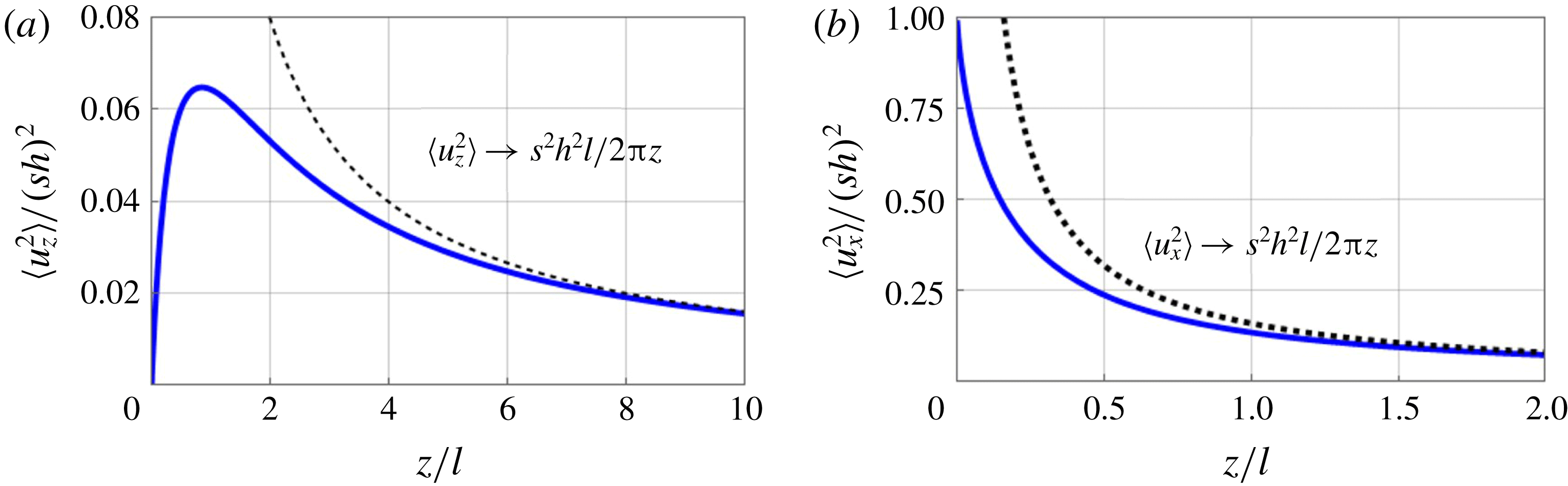
As mentioned above, the near-field velocity is sensitive to the roughness structure. However, as is clear from (4.1)–(4.3), various surfaces produce flow patterns with common qualitative features. In particular, the intensity
 $\langle u_{z}^{2}\rangle$
of fluctuations in wall-normal velocity as a function of distance from the wall is always non-monotonic, taking its maximum at a distance of the order of the roughness correlation length
 $l$
– see figure 2(a) for illustration. In contrast, the dependence of the fluctuation intensity
 $\langle u_{x}^{2}\rangle$
on the distance from the wall is usually monotonic and then it takes its maximum value on the wall – see figure 2(b). Interestingly, the locations of these maximum values are completely independent of the characteristic height
 $h$
of surface imperfections. On the other hand, the maximum values do not depend on
 $l$
, but are determined only by
 $h$
.
The wall-normal profile of fluctuation intensities
 $\langle u_{z}^{2}\rangle$
and
 $\langle u_{x}^{2}\rangle$
(panels (a) and (b), respectively) for the exponential surface autocorrelation function
 $F(r)=h^{2}\text{e}^{-|r|/l}$
. The solid lines were obtained numerically by using (4.2) and (4.3). The dashed lines represent the asymptotic dependence (4.5) at
 $z\gg l$
.

This conclusion agrees well with those reported before. For example, in Zayernouri et al. (Reference Zayernouri, Park, Tartakovsky and Karniadakis2013) the Stokes flow in a channel with a rough wall was solved numerically and it was found that the location of the maximum of fluctuations in wall-normal velocity moves towards the rough wall as the correlation length decreases and is insensitive to the roughness variance. Similar features have been observed for the deterministic roughness in the form of sinusoidal waviness for channel flows with moderate Reynolds number (see Wang et al.
Reference Wang, Wang and Zhang2005; Wang & Wang Reference Wang and Wang2007). Namely, the increase of the wall wavenumber is shown to result in a decrease of the disturbance area of the flow field, while the relative roughness determines the maximum disturbance amplitude, but does not affect the width of the disturbed area. Note also that, in the vicinity of the wall, the streamwise component of velocity predominates in the intensity of velocity fluctuations,
 $\langle u_{x}^{2}\rangle \gg \langle u_{z}^{2}\rangle$
, while in the far-field region,
 $z\gg l$
, the two components are equal to each other (see expression (4.5)).
As for the spatial decay of correlations in flow fluctuations, the velocity correlation length in the region
 $z\lesssim l$
is of the order of
 $l$
. The energy spectrum of fluctuations (6.9) at
 $h\ll z\lesssim l$
is determined by the power spectral density function of surface roughness
 $\tilde{F}(k)$
, which is the Fourier transform of the surface autocorrelation function
 $F(r)$
. For example, for exponential correlator
 $F(r)=h^{2}\text{e}^{-|r|/l}$
, which is typical for most etched surfaces, we have
 $\tilde{F}(k)=2h^{2}l/(k^{2}l^{2}+1)$
and, therefore, the near-field spectrum displays a power law with exponent equal to
 $-2$
in the region
 $1/z\gg k\gg 1/l$
and decays exponentially when
 $k\gg 1/z$
.
The dependence of velocity fluctuations on the roughness statistics in the near-wall region allows us to propose the hydrodynamic method of investigation of surface properties: measuring the energy spectrum of velocity fluctuations
 $E(k)$
and using expression (6.9), one can infer the power spectral density function
 $\tilde{F}(k)$
of the surface.
8 Three-dimensional flow over a flat surface
The perturbative approach can be applied to the fluctuations in 3D flow produced by an imperfect wall whose surface
 $z=\unicode[STIX]{x1D709}(x,y)$
is stochastically rough in both streamwise and spanwise directions. Now the spatial velocity fluctuations are given by (Jansons & Lister Reference Jansons and Lister1988)
 $$\begin{eqnarray}\displaystyle u_{x}(x,y,z)=-\frac{3sz}{2\unicode[STIX]{x03C0}}\int _{-\infty }^{+\infty }\int _{-\infty }^{+\infty }\frac{\text{d}x^{\prime }\,\text{d}y^{\prime }\,(x-x^{\prime })^{2}\unicode[STIX]{x1D709}(x^{\prime },y^{\prime })}{((x-x^{\prime })^{2}+(y-y^{\prime })^{2}+z^{2})^{5/2}}, & & \displaystyle\end{eqnarray}$$
 $$\begin{eqnarray}\displaystyle u_{y}(x,y,z)=-\frac{3sz}{2\unicode[STIX]{x03C0}}\int _{-\infty }^{+\infty }\int _{-\infty }^{+\infty }\frac{\text{d}x^{\prime }\,\text{d}y^{\prime }\,(x-x^{\prime })(y-y^{\prime })\unicode[STIX]{x1D709}(x^{\prime },y^{\prime })}{((x-x^{\prime })^{2}+(y-y^{\prime })^{2}+z^{2})^{5/2}}, & & \displaystyle\end{eqnarray}$$
 $$\begin{eqnarray}\displaystyle u_{z}(x,y,z)=-\frac{3sz^{2}}{2\unicode[STIX]{x03C0}}\int _{-\infty }^{+\infty }\int _{-\infty }^{+\infty }\frac{\text{d}x^{\prime }\,\text{d}y^{\prime }\,(x-x^{\prime })\unicode[STIX]{x1D709}(x^{\prime },y^{\prime })}{((x-x^{\prime })^{2}+(y-y^{\prime })^{2}+z^{2})^{5/2}}. & & \displaystyle\end{eqnarray}$$
Note that, if the surface elevation
 $\unicode[STIX]{x1D709}(x,y)$
does not depend on the
 $y$
-coordinate, then the integration over the spanwise direction can be performed and one obtains the previously found result (3.8). Further, we will assume that the roughness statistics are homogeneous and isotropic.
In the far-field region,
 $z\gg l$
, the velocity fluctuations have the Gaussian probability density function
 $P(\boldsymbol{u})=((2\unicode[STIX]{x03C0})^{3}\det \hat{\unicode[STIX]{x1D72E}})^{-1/2}\exp (-(1/2)\boldsymbol{u}^{\text{T}}\hat{\unicode[STIX]{x1D72E}}^{-1}\boldsymbol{u})$
, which is also the consequence of the central limit theorem; see § 5. The elements of the covariance matrix
 $\unicode[STIX]{x1D6F4}_{ij}=\langle u_{i}u_{j}\rangle$
are given by
 $$\begin{eqnarray}\displaystyle \langle u_{x}^{2}\rangle =\frac{9As^{2}}{128\unicode[STIX]{x03C0}z^{2}},\quad \langle u_{y}^{2}\rangle =\frac{3As^{2}}{128\unicode[STIX]{x03C0}z^{2}},\quad \langle u_{z}^{2}\rangle =\frac{3As^{2}}{32\unicode[STIX]{x03C0}z^{2}}, & & \displaystyle\end{eqnarray}$$
 $$\begin{eqnarray}\displaystyle \langle u_{x}u_{y}\rangle =\langle u_{x}u_{z}\rangle =\langle u_{y}u_{z}\rangle =0. & & \displaystyle\end{eqnarray}$$
Compare this with the result (4.5) obtained for 2D geometry. Now the quantity
 $A$
is estimated as
 $h^{2}l^{2}$
, where as before
 $h$
and
 $l$
denote the roughness height of the surface and its correlation length, respectively.
The velocity correlation tensor is defined by
 $\unicode[STIX]{x1D619}_{ij}(\boldsymbol{r},z_{1},z_{2})=\langle u_{i}(\mathbf{0},z_{1})u_{j}(\boldsymbol{r},z_{2})\rangle$
where
 $\boldsymbol{r}=(x,y)$
is the vector in the
 $x{-}y$
plane. As in the 2D case, velocity correlations at
 $z_{1},z_{2}\gg l$
exhibit algebraic decay in streamwise, spanwise and wall-normal directions. The energy spectrum
 $E(\boldsymbol{k})$
of velocity fluctuations is determined by the trace of the correlation tensor in Fourier space, namely
 $$\begin{eqnarray}E(\boldsymbol{k})=\frac{1}{8\unicode[STIX]{x03C0}^{2}}(\tilde{R}_{xx}(\boldsymbol{k},z,z)+\tilde{R}_{yy}(\boldsymbol{k},z,z)+\tilde{R}_{zz}(\boldsymbol{k},z,z)),\end{eqnarray}$$
where
 $\tilde{\unicode[STIX]{x1D619}}_{ij}(\boldsymbol{k},z_{1},z_{2})=\int _{-\infty }^{+\infty }\unicode[STIX]{x1D619}_{ij}(\boldsymbol{r},z_{1},z_{2})\text{e}^{-\text{i}\boldsymbol{k}\boldsymbol{r}}\,\text{d}^{2}\boldsymbol{r}$
and
 $\boldsymbol{k}=(k_{x},k_{y})$
. After straightforward calculations (see appendix B) one finds
 $$\begin{eqnarray}E(\boldsymbol{k})=\frac{s^{2}}{8\unicode[STIX]{x03C0}^{2}}\tilde{F}(k)\left(1-2\frac{k_{x}^{2}}{k}z+2k_{x}^{2}z^{2}\right)\text{e}^{-2kz},\end{eqnarray}$$
where we have introduced
 $k=|\boldsymbol{k}|$
. Note that by substituting
 $k_{y}=0$
, we can restore the previously obtained answer (6.9) for the 2D problem.
In experimental papers, the energy spectrum
 $E_{av}(k)$
averaged over the direction of the vector
 $\boldsymbol{k}$
is often calculated,
 $$\begin{eqnarray}E_{av}(k)=k\int _{0}^{2\unicode[STIX]{x03C0}}\text{d}\unicode[STIX]{x1D711}\,E(\boldsymbol{k}),\end{eqnarray}$$
where the integration is performed over the polar angle in the
 $k_{x}{-}k_{y}$
plane. By substituting expression (8.7) into (8.8), we obtain
 $$\begin{eqnarray}E_{av}(k)=\frac{s^{2}}{4\unicode[STIX]{x03C0}}\tilde{F}(k)(1-kz+k^{2}z^{2})k\text{e}^{-2kz}.\end{eqnarray}$$
In the case of the exponential surface autocorrelation function
 $F(r)=h^{2}\text{e}^{-|r|/l}$
, one has
 $\tilde{F}(k)=2\unicode[STIX]{x03C0}h^{2}l^{2}/(k^{2}l^{2}+1)^{3/2}$
and, therefore, the near-field spectrum averaged over angle,
 $E_{av}(k)$
, displays a power-law tail with exponent equal to
 $-2$
in the region
 $1/z\gg k\gg 1/l$
and decays exponentially when
 $k\gg 1/z$
.
9 Flow between two plates
In many practical situations, the correlation length of surface irregularities is of the order of the channel diameter so that the roughness cannot be treated as shortly correlated. What can one say about the interplay between the roughness statistics and flow behaviour in this case? The scheme presented here allows one to address questions of this kind as well. Motivated by the experiment of Jaeger et al. (Reference Jaeger, Ren, Xie, Sundararajan, Olsen and Ganapathysubramanian2012), in this section we consider the Stokes flow in a plane channel of width
 $d\gg h$
. The bottom wall of the channel, which corresponds to
 $z=\unicode[STIX]{x1D709}(x)$
, is rough, while the top wall,
 $z=d$
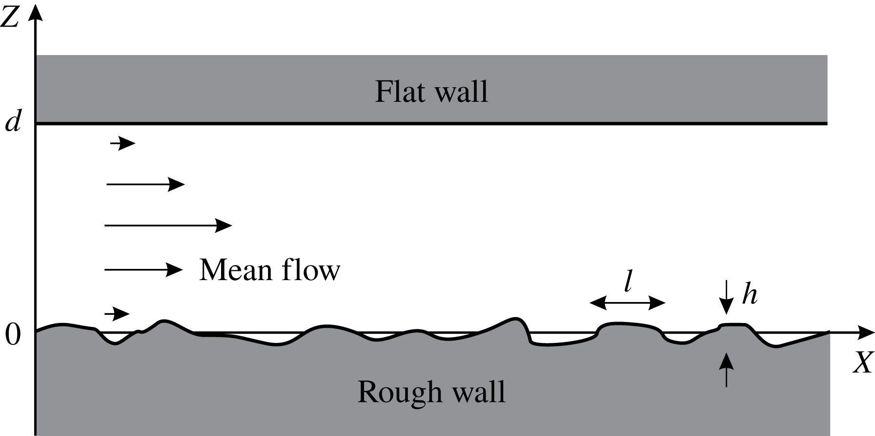
, is perfectly flat (see figure 3). First, we consider the 2D model; the generalization to three dimensions is straightforward.
Viscous fluid flow between a no-slip rough wall and a no-slip perfectly flat wall.

9.1 Two-dimensional plane channel
The fluid flow in the channel is created by applying the pressure gradient
 $\unicode[STIX]{x1D735}P_{0}$
along the
 $x$
-direction. The solution of the problem without roughness is the well-known Poiseuille flow
 $$\begin{eqnarray}U_{x}(z)=sz(1-z/d),\quad s=-\frac{\unicode[STIX]{x1D735}P_{0}}{2\unicode[STIX]{x1D702}}d,\end{eqnarray}$$
and then the roughness-induced velocity correction
 $\boldsymbol{u}$
must satisfy the same boundary value problem (3.2)–(3.3), but with the additional no-slip condition
 $\boldsymbol{u}|_{z=d}=0$
, which is posed on the top wall. Note again that the used perturbative approach is correct only in the limit of small-amplitude roughness, when the characteristic height
 $h$
of the surface imperfections is much smaller than their characteristic transverse size,
 $l\gg h$
. Note also that the considered first-order perturbation theory preserves the discharge of fluid as compared to the unperturbed flow. The effect of the decrease of the mean flow rate (Phan-Thien Reference Phan-Thien1980) or an effective slip (Panzer, Liu & Einzel Reference Panzer, Liu and Einzel1992) appears only in the second order with respect to
 $h/l\ll 1$
and we refer the interested readers to these publications for details.
The considered boundary value problem can be solved in Fourier space,
 $\tilde{f}(q_{x},z)=\int _{-\infty }^{+\infty }\text{d}x\hspace{2.22198pt}f(x,z)\text{e}^{-\text{i}q_{x}x}$
, and then for the velocity fluctuations one obtains
 $$\begin{eqnarray}\displaystyle \tilde{u} _{x} & = & \displaystyle \frac{s\tilde{\unicode[STIX]{x1D709}}}{1+2d^{2}q^{2}-\cosh (2dq)}\{\cosh (q(2d-z))+[2dq^{2}(z-d)-1]\cosh (qz)\nonumber\\ \displaystyle & & \displaystyle -\,qz\sinh (q(2d-z))+q(2d-z)\sinh (qz)\},\end{eqnarray}$$
 $$\begin{eqnarray}\displaystyle \tilde{u} _{z} & = & \displaystyle \frac{-\text{i}q_{x}s\tilde{\unicode[STIX]{x1D709}}}{1+2d^{2}q^{2}-\cosh (2dq)}\{z\cosh (q(2d-z))-z\cosh (qz)\nonumber\\ \displaystyle & & \displaystyle +\,2dq(z-d)\sinh (qz)\},\end{eqnarray}$$
where we denote the wavenumber by
 $q=|q_{x}|$
. The important characteristic of the fluid flow is the energy spectrum of velocity fluctuations
 $E(k)$
, which was defined by expression (6.8). Now it is equal to
 $$\begin{eqnarray}E(k)=\frac{1}{8\unicode[STIX]{x03C0}^{2}}\int _{-\infty }^{+\infty }\,\text{d}q\,\langle \tilde{u} _{x}(q)\tilde{u} _{x}(k)+\tilde{u} _{z}(q)\tilde{u} _{z}(k)\rangle ,\end{eqnarray}$$
and by using
 $\langle \tilde{\unicode[STIX]{x1D709}}_{q}\tilde{\unicode[STIX]{x1D709}}_{k}\rangle =2\unicode[STIX]{x03C0}\unicode[STIX]{x1D6FF}(k+q)\tilde{F}(k)$
, we find
 $$\begin{eqnarray}\displaystyle E(k) & = & \displaystyle \frac{s^{2}\tilde{F}(k)}{4\unicode[STIX]{x03C0}[1+2d^{2}k^{2}-\cosh (2dk)]^{2}}\big[\{\cosh (k(2d-z))-kz\sinh (k(2d-z))\nonumber\\ \displaystyle & & \displaystyle +\,(2dk^{2}(z-d)-1)\cosh (kz)+k(2d-z)\sinh (kz)\}^{2}\nonumber\\ \displaystyle & & \displaystyle +\,k^{2}\{-z\cosh (kz)+2dk(z-d)\sinh (kz)+z\cosh (k(2d-z))\}^{2}\big].\end{eqnarray}$$
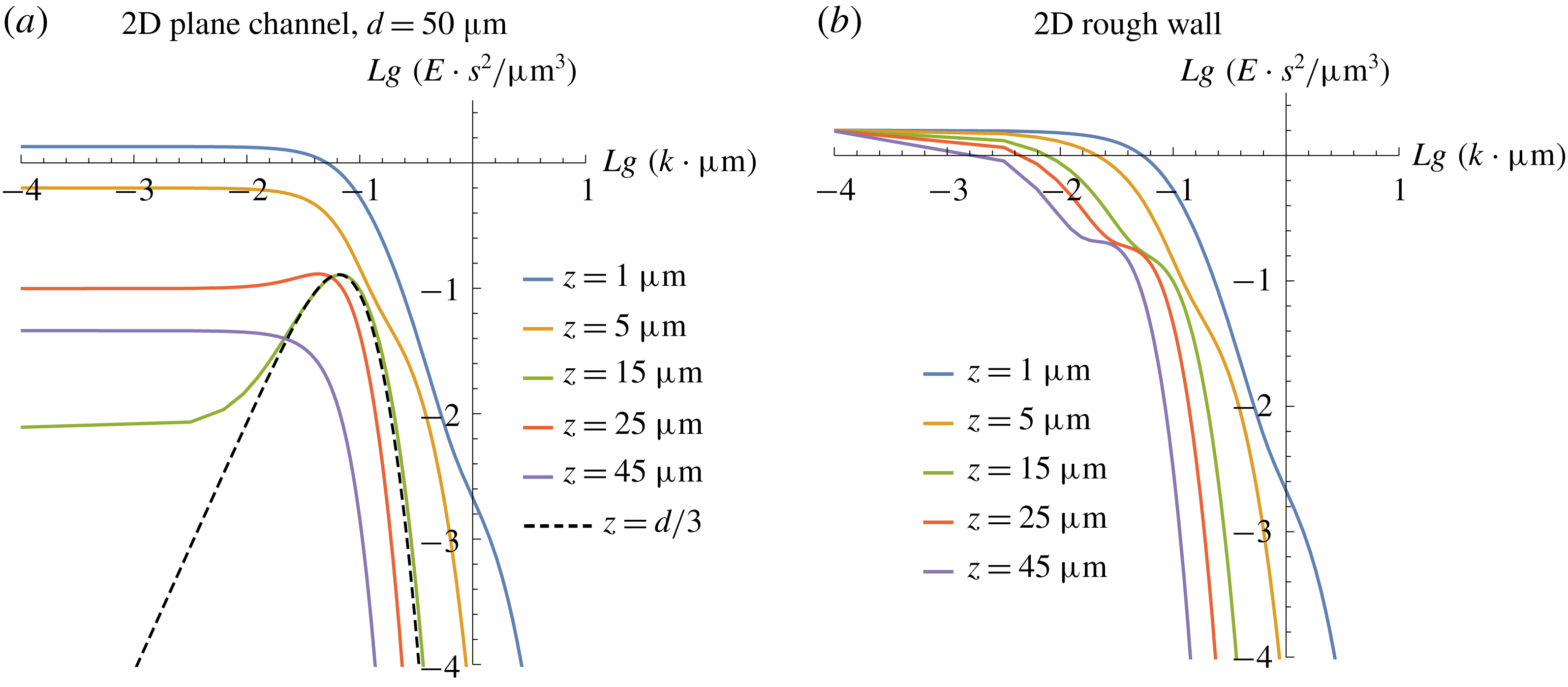
(a) The energy spectrum (9.5) in a channel of width
 $d=50~\unicode[STIX]{x03BC}\text{m}$
and (b) the energy spectrum (6.9) for the flow over a plane depending on the distance
 $z$
to the rough wall. In both cases the surface imperfections are correlated exponentially,
 $F(r)=h^{2}\text{e}^{-|r|/l}$
, with the parameter
 $l=10~\unicode[STIX]{x03BC}\text{m}$
. Numerical values correspond to the parameter
 $sh=1~\unicode[STIX]{x03BC}\text{m}/s$
.

To illustrate expression (9.5), we consider the fluid flow in a plane channel of width
 $d=50~\unicode[STIX]{x03BC}\text{m}$
, assuming that surface imperfections on the bottom wall have exponential correlation function
 $F(r)=h^{2}\text{e}^{-|r|/l}$
with the parameter
 $l=10~\unicode[STIX]{x03BC}\text{m}$
. The dependence of the energy spectrum
 $E(k)$
of velocity fluctuations on distance
 $z$
to the bottom wall is presented in figure 4(a). For comparison, figure 4(b) shows a similar spectrum (6.9) for the fluid flow over a rough wall.
Near the rough wall,
 $z\ll d$
, both energy spectra look identical, because at small
 $z$
the flow in the channel does not feel the presence of the second wall. The rough wall is able to generate fluctuation with
 $k\lesssim 1/l$
and this point corresponds to the kink in the spectra. The small bend on curves
 $z=1~\unicode[STIX]{x03BC}\text{m}$
in figure 4(a,b) near point
 $\lg k=0$
corresponds to the change in asymptotic behaviour, which was discussed in § 7. In the region
 $k\gg 1/z$
one obtains
 $E(k)\propto \text{e}^{-2kz}$
, while in the region
 $1/l\ll k\ll 1/z$
one has
 $E(k)\propto k^{-2}$
. Far from the wall, when
 $z>l$
, we observe only exponential decay.
As the distance to the rough wall increases, the energy spectra become different. First, the channel suppresses large-scale fluctuations; see curves
 $z=5~\unicode[STIX]{x03BC}\text{m}$
. At distance
 $z\sim (0.2{-}0.5)d$
, the spectrum in the channel becomes non-monotonic and exhibits a maximum; see curve
 $z=15~\unicode[STIX]{x03BC}\text{m}$
. The appearance of a maximum and its position are weakly dependent on the correlation length
 $l\lesssim d$
. Thus, the width
 $d$
of the channel imposes some restrictions on the size of fluctuations that are able to penetrate inside the depth.
Interestingly, the large-scale velocity fluctuations in the channel are completely suppressed, i.e.
 $E(k)\rightarrow 0,~k\rightarrow 0$
, at a certain distance
 $z=d/3$
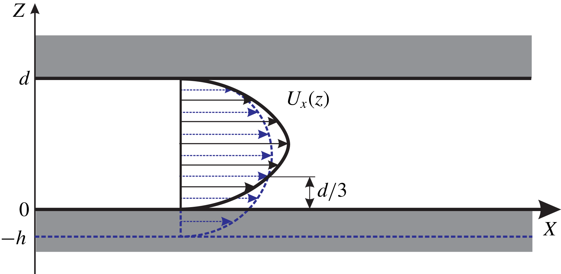
from the bottom wall; see dashed line in figure 4(a). This result can be explained in the following way. Owing to the linearity of the problem, the large-scale velocity fluctuations are generated by the large-scale surface imperfections. Clearly, a surface asperity whose amplitude is
 $h$
and streamwise size is much larger than
 $d$
, locally changes the channel width as shown in figure 5. The used perturbative approach preserves the discharge of fluid in the linear approximation with respect to the surface elevation
 $h\ll d$
. Therefore, the velocity field for the channel with modified width is
 $$\begin{eqnarray}v_{x}(z)=s\frac{d^{3}}{(d+h)^{3}}(z+h)(1-z/d),\quad v_{z}=0,\end{eqnarray}$$
where
 $z=-h$
corresponds to the new position of the bottom wall. The obtained velocity profile intersects with the solution of the problem without roughness (9.1a,b
) in the point
 $z=d/3$
, and therefore there are no large-scale velocity fluctuations at this distance from the rough wall.
Schematic picture that explains the total suppression of large-scale velocity fluctuations in the channel at a distance
 $z=d/3$
from the rough wall. The solid curve represents the velocity field (9.1a,b
) for the problem without roughness, and the dashed curve shows the velocity field (9.6) modified by large-scale surface imperfection.

Further increasing the distance to the wall, one can see that the value
 $E(k)$
in the maximum practically does not change, while the energy density of large-scale fluctuations increases by an order of magnitude; see curve
 $z=25~\unicode[STIX]{x03BC}\text{m}$
in figure 4(a). After the maximum disappears, the spectrum gradually decreases for all wavenumbers with increasing distance to the bottom wall, turning to zero on the top perfectly flat wall.
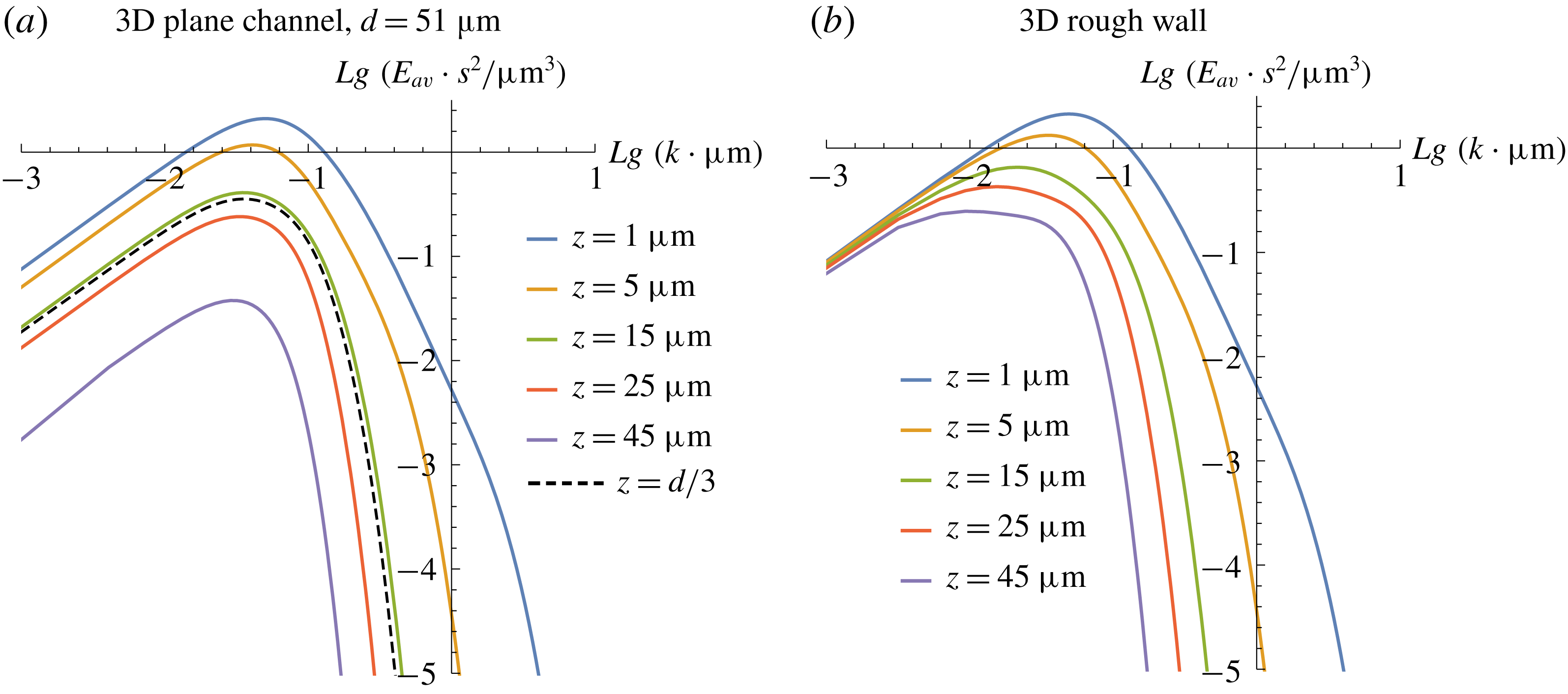
(a) The energy spectrum
 $E_{av}(k)$
in a 3D channel of width
 $d=51~\unicode[STIX]{x03BC}\text{m}$
and (b) the energy spectrum (8.9) for the 3D flow over a plane depending on the distance
 $z$
to the rough wall. In both cases the surface imperfections are correlated exponentially,
 $F(r)=h^{2}\text{e}^{-|r|/l}$
, with the parameter
 $l=12.9~\unicode[STIX]{x03BC}\text{m}$
. Numerical values correspond to the parameter
 $sh=1~\unicode[STIX]{x03BC}\text{m}/s$
.

9.2 Three-dimensional plane channel
Experimentally, the energy spectrum was measured in a channel between two parallel plates in Jaeger et al. (Reference Jaeger, Ren, Xie, Sundararajan, Olsen and Ganapathysubramanian2012). However, in that work, the bottom plate was stochastically rough in both streamwise and spanwise directions. Our approach can be straightforwardly generalized to this case as well. To implement the direct comparison, now we consider the 3D plane channel of width
 $d=51~\unicode[STIX]{x03BC}\text{m}$
, and the correlation function of surface imperfections on the rough wall is assumed to be exponential,
 $F(r)=h^{2}\text{e}^{-|r|/l}$
, with the parameter
 $l=12.9~\unicode[STIX]{x03BC}\text{m}$
. The r.m.s. of surface fluctuations was equal to
 $h=19~\text{nm}\ll l$
and thus the perturbative approach is well justified.
The energy spectrum of velocity fluctuations (8.8) in the 3D plane channel is shown in figure 6(a) for different distances
 $z$
to the rough wall. For comparison, figure 6(b) shows a similar spectrum (8.9) for the 3D fluid flow over a rough plane. The large-scale behaviour,
 $k\rightarrow 0$
, is described by
 $E_{av}(k)\propto k$
due to the phase volume factor, arising from averaging over the angle in the
 $k_{x}{-}k_{y}$
plane; see expression (8.8). One can see that the channel suppresses large-scale fluctuations as in the 2D case, but now the distance
 $z=d/3$
does not play any special role, because the fluid flow has an additional degree of freedom and the flow rate can depend on the
 $y$
-coordinate. The small-scale behaviour demonstrates two regimes, as we have discussed in § 8. In the region
 $k\gg 1/z$
one observes
 $E_{av}(k)\propto \text{e}^{-2kz}$
, while in the region
 $1/l\ll k\ll 1/z$
one has
 $E_{av}(k)\propto k^{-2}$
. The last intermediate asymptotic can be observed only near the rough wall; see curves
 $z=1~\unicode[STIX]{x03BC}\text{m}$
in figure 6. Far from the wall, when
 $z>l$
, the decay is exponential.
We must conclude that our theoretical findings are different from the results of experimental measurements that are presented in Jaeger et al. (Reference Jaeger, Ren, Xie, Sundararajan, Olsen and Ganapathysubramanian2012). The experimental spectrum is monotonic, while our theoretical analysis shows that the spectrum has a maximum (see figure 6
a). Qualitatively, the large-scale behaviour demonstrates a reasonable agreement, while the small-scale behaviour is completely different. We would like to stress that the predicted exponential decay
 $\propto \text{e}^{-2kz}$
of small-scale fluctuations is natural. Owing to the linearity of the problem, the velocity fluctuations with wavenumber
 $k$
are generated by the surface imperfections with the same wavenumber, and therefore their decay is exponential; see expression (4.6). We do not know how to explain the absence of an exponential decay in the experimental data. In part, the discrepancy between the theory and the measurements can be attributed to the speculation that the pair correlation function of surface
 $F(r)$
is not exponential, but has a more complex structure and depends on several scales. This speculation is based on the results of the experiment, in which the presence of several characteristic scales can be observed.
10 Dispersion of passive scalar
In this section we consider transport of the passive scalar in the steady velocity field with a relatively weak random component generated by the wall imperfections in the direction perpendicular to the wall. As above we write the fluid velocity as
 $\boldsymbol{v}=\boldsymbol{U}+\boldsymbol{u}$
, where
 $\boldsymbol{U}=(U_{x}(z),0)$
represents the regular flow and
 $\boldsymbol{u}$
is the spatially random perturbation. We start with the 2D fluid flow over the rough plane and then we will briefly discuss other considered geometries as well. The passive tracer evolution is governed by the interplay of spatially varying mean flow and flow fluctuations
 $$\begin{eqnarray}\unicode[STIX]{x2202}_{t}\unicode[STIX]{x1D703}+(\boldsymbol{U}+\boldsymbol{u})\unicode[STIX]{x1D735}\unicode[STIX]{x1D703}=0.\end{eqnarray}$$
Here we have omitted the molecular diffusion term because we would like to focus on the mass transport produced only by the roughness-induced velocity fluctuations. A formal solution of (10.1) is well known. The advection occurs along characteristics
 $\unicode[STIX]{x1D746}(\boldsymbol{r},t)$
that have to be determined by solving the system of equations
 $$\begin{eqnarray}\unicode[STIX]{x2202}_{t}\unicode[STIX]{x1D746}=\boldsymbol{U}(\unicode[STIX]{x1D746})+\boldsymbol{u}(\unicode[STIX]{x1D746})\end{eqnarray}$$
with corresponding initial condition.
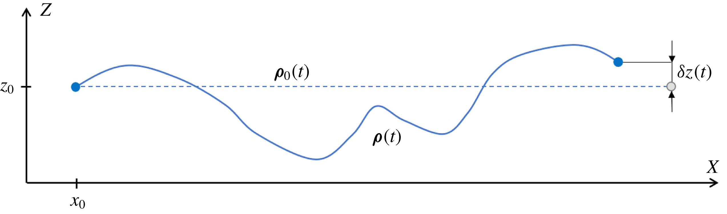
The advection of the passive tracer along the characteristic
 $\unicode[STIX]{x1D746}(t)$
. The dashed line corresponds to the advection only by the mean flow
 $U_{x}(z)$
.

Let us find the displacement
 $\unicode[STIX]{x1D6FF}z(t)$
of the passive tracer in the wall-normal direction, assuming that initially it was located at some point
 $(x_{0},z_{0})$
; see figure 7. Since the roughness-induced fluctuations are significantly smaller than the mean flow, we can solve (10.2) within the framework of the perturbation theory, i.e.
 $\unicode[STIX]{x1D746}=\unicode[STIX]{x1D746}_{0}+\unicode[STIX]{x1D746}_{1}+\cdots \,$
, where
 $$\begin{eqnarray}\displaystyle \unicode[STIX]{x2202}_{t}\unicode[STIX]{x1D746}_{0}=\boldsymbol{U}(\unicode[STIX]{x1D746}_{0}),\quad \unicode[STIX]{x1D746}_{0}(0)=(x_{0},z_{0}), & & \displaystyle\end{eqnarray}$$
 $$\begin{eqnarray}\displaystyle \unicode[STIX]{x2202}_{t}\unicode[STIX]{x1D70C}_{1i}=\unicode[STIX]{x2202}_{k}U_{i}(\unicode[STIX]{x1D746}_{0})\unicode[STIX]{x1D70C}_{1k}+u_{i}(\unicode[STIX]{x1D746}_{0}),\quad \unicode[STIX]{x1D746}_{1}(0)=(0,0). & & \displaystyle\end{eqnarray}$$
The solution is
 $\unicode[STIX]{x1D746}_{0}=(x_{0}+U_{0}t,z_{0})$
where
 $U_{0}=U_{x}(z_{0})$
, which corresponds to the advection by the mean flow, and for the first-order correction we find
 $$\begin{eqnarray}\unicode[STIX]{x1D6FF}z(t)\approx \unicode[STIX]{x1D70C}_{1z}(t)=\int _{0}^{t}\text{d}\unicode[STIX]{x1D70F}\,u_{z}(x_{0}+U_{0}\unicode[STIX]{x1D70F},z_{0}).\end{eqnarray}$$
Note that, to calculate the second-order correction to
 $\unicode[STIX]{x1D6FF}z(t)$
, one should not only find
 $\unicode[STIX]{x1D70C}_{2z}(t)$
but also modify the initial scheme (3.2)–(3.3), taking into account terms of the second order in the surface elevation
 $\unicode[STIX]{x1D709}(x)$
.
Next, we will assume that
 $z_{0}\gg l$
and therefore, as we explained earlier, the statistical properties of velocity fluctuations are insensitive to the fine details of the roughness statistics and the characteristic length scale in which correlation between fluctuation decays is of the order of the distance to the wall
 $z_{0}$
. The expression (10.5) is correct until
 $U_{0}t\ll z_{0}\sqrt{U_{0}/u}$
, where
 $u$
is the characteristic magnitude of velocity fluctuations; see (4.5). Otherwise, one has to take into account the contribution to
 $\unicode[STIX]{x1D6FF}z(t)$
produced by the second-order term
 $\unicode[STIX]{x1D70C}_{2z}(t)$
. By using expression (10.5) and averaging over the roughness statistics, we obtain
 $\langle \unicode[STIX]{x1D6FF}z(t)\rangle =0$
and
 $$\begin{eqnarray}\langle \unicode[STIX]{x1D6FF}z(t)^{2}\rangle =\frac{1}{U_{0}^{2}}\int _{0}^{U_{0}t}\text{d}\unicode[STIX]{x1D701}\int _{-\unicode[STIX]{x1D701}}^{\unicode[STIX]{x1D701}}\text{d}\unicode[STIX]{x1D702}\,\langle u_{z}(0,z_{0})u_{z}(\unicode[STIX]{x1D702},z_{0})\rangle .\end{eqnarray}$$
By substituting expression (6.5) and
 $U_{0}=sz_{0}$
, for the 2D fluid flow over the rough plane we finally obtain
 $$\begin{eqnarray}\langle \unicode[STIX]{x1D6FF}z(t)^{2}\rangle =\frac{A}{\unicode[STIX]{x03C0}z_{0}}\frac{(st)^{2}}{(st)^{2}+4},\quad st\ll \sqrt{U_{0}/u}.\end{eqnarray}$$
This means that the spatial dispersion in the wall-normal direction sufficiently quickly reaches the value
 $\langle \unicode[STIX]{x1D6FF}z^{2}\rangle _{lim}=A/(\unicode[STIX]{x03C0}z_{0})$
and no longer changes with time. As
 $h\ll l\ll z_{0}$
and
 $A\sim h^{2}l$
, we obtain the estimate
 $\langle \unicode[STIX]{x1D6FF}z^{2}\rangle _{lim}\sim h^{2}l/z_{0}\ll z_{0}^{2}$
. Therefore, the roughness-induced velocity fluctuations do not lead to the enhancement of diffusion of the passive scalar in the direction perpendicular to the wall at least in the leading-order approximation considered here.
In principle, expression (10.6) can be used to estimate the asymptotic value
 $\langle \unicode[STIX]{x1D6FF}z^{2}\rangle _{lim}$
at any distance
 $z_{0}$
to the wall and for any geometry considered in this paper. The main contribution to the integrals comes from the scale of the correlation length of velocity fluctuations
 $l_{corr}=\max (z_{0},l)$
and then
 $$\begin{eqnarray}\langle \unicode[STIX]{x1D6FF}z^{2}\rangle _{lim}\sim \frac{\langle u_{z}^{2}\rangle }{U_{0}^{2}}l_{corr}^{2}.\end{eqnarray}$$
By using expression (4.5), one can check that the estimation correctly reproduces the asymptotic value of dispersion for the 2D flow over a rough wall in the far-field region. Note that for the 3D flow in the same geometry one can obtain
 $\langle \unicode[STIX]{x1D6FF}z^{2}\rangle _{lim}\sim A/z_{0}^{2}$
,
 $z_{0}\gg l$
, where
 $A\sim h^{2}l^{2}$
and we have used expression (8.4).
11 Conclusion
We have investigated the influence of stochastic boundary roughness on the stationary Stokes flow of an incompressible fluid in the limit when the typical height
 $h$
of the random asperities of the boundary is much smaller than their transverse size
 $l$
. The focus of the paper is on the statistical properties of the spatially random flow component produced in the presence of roughness. Being small compared with the mean flow far enough from the boundaries, the fluctuations in fluid velocity can be treated perturbatively there.
First, we considered the fluid flow in a half-space over a flat imperfect wall in both two and three spatial dimensions. While the near-wall properties of the fluid velocity fluctuations are sensitive to the statistics of wall roughness, universal behaviour emerges in the far field. Namely, as long as the variance of surface height is finite, the velocity fluctuations at distance
 $z\gg l$
from the wall possess Gaussian statistics. The far-field intensity of fluctuations as a function of distance from the wall exhibits a power-law decay with a dimension-dependent exponent that is insensitive to the details of the roughness statistics. In addition, we calculated the two-point correlation function and the energy spectrum of the velocity fluctuations, revealing the power-law decay of spatial correlations.
Next, we considered the 2D and 3D flow in the plane channel between two parallel walls, one of which is rough, while the other is perfectly flat. Particular attention was paid to the energy spectrum of velocity fluctuations as a function of the distance to the rough wall. The analytical expression (9.5) for the energy spectrum is valid for any relation between the correlation length
 $l$
of imperfect wall roughness and the distance
 $d$
between the channel walls. The main difference in comparison with the half-space geometry is the suppression of the large-scale velocity fluctuations inside the channel.
Finally, we considered the transport of a passive scalar in the steady velocity field with a relatively weak random component generated by the wall imperfections. It turns out that the spatial dispersion of the passive scalar in the wall-normal direction reaches some value given by expression (10.8) on a time scale of the order of the inverse shear rate of the mean flow, and no longer changes with time. Therefore, random surface roughness does not lead to the enhancement of diffusion of the passive scalar in the direction perpendicular to the wall, at least in the second order with respect to the roughness amplitude. Qualitatively, this result is explained by the fact that Lagrangian trajectories of the laminar flow in the channel with small-amplitude wall roughness do not diverge as the streamwise coordinate grows.
We hope that the obtained results will motivate further work on the impact of random roughness on microfluidic flow behaviour. Various experimental tools have been successfully applied for roughness characterization (see Yu et al. Reference Yu, Cao, Namba and Ma1996; Yilbas & Hasmi Reference Yilbas and Hasmi1999; Bhushan Reference Bhushan2001; Duparre et al. Reference Duparre, Ferre-Borrull, Gliech, Notni, Steinert and Bennett2002; Zhu & Zhang Reference Zhu and Zhang2004; Kuo & Chao Reference Kuo and Chao2010; Ren et al. Reference Ren, Ganapathysubramanian and Sundararajan2011). The laminar velocity field inside microfluidic channels with micro/nanoscale surface roughness can be measured with the particle image velocimetry technique (Silva, Leal & Semiao Reference Silva, Leal and Semiao2008; Jaeger et al. Reference Jaeger, Ren, Xie, Sundararajan, Olsen and Ganapathysubramanian2012; Ren Reference Ren2013). That encourages us to think that an experimental test of our findings is a matter for the near future.
Acknowledgement
We thank S. S. Vergeles for valuable discussions. This work was supported by the Russian Science Foundation, grant no. 14-22-00259.
Appendix A. Characteristic function
By using the functional methods, we can express the characteristic function through the integration over different realizations of the surface elevation
 $\unicode[STIX]{x1D709}(x)$
,
 $$\begin{eqnarray}G(\boldsymbol{k})=\int {\mathcal{D}}\unicode[STIX]{x1D709}{\mathcal{Q}}(\unicode[STIX]{x1D709})\text{e}^{\text{i}\boldsymbol{k}\boldsymbol{\cdot }\boldsymbol{u}[\unicode[STIX]{x1D709}]},\end{eqnarray}$$
where the velocity
 $\boldsymbol{u}[\unicode[STIX]{x1D709}]$
should be taken at some fixed point. Without loss of generality we assume that this point has coordinates
 $(0,z)$
. We also assume that
 $z\gg l$
and it means that the random heights
 $\unicode[STIX]{x1D709}(x)$
of surface asperities at different points of the wall can be considered as completely independent from each other.
To illustrate the functional integration we will use discretization. We split the wall surface into many small pieces and then the streamwise coordinate takes discrete values
 $x_{k}=k\unicode[STIX]{x1D700}$
, where
 $k$
is an integer and
 $\unicode[STIX]{x1D700}$
is the discretization step,
 $z\gg \unicode[STIX]{x1D700}\gtrsim l$
. For the characteristic function we obtain
 $$\begin{eqnarray}G(\boldsymbol{k})=\mathop{\prod }_{k}\int \text{d}\unicode[STIX]{x1D709}_{k}\,P(\unicode[STIX]{x1D709}_{k})\text{e}^{\text{i}\unicode[STIX]{x1D700}\unicode[STIX]{x1D6FC}(x_{k})\unicode[STIX]{x1D709}_{k}},\quad \unicode[STIX]{x1D6FC}(x_{k})=\frac{2sz}{\unicode[STIX]{x03C0}}\frac{x_{k}(zk_{z}-x_{k}k_{x})}{(x_{k}^{2}+z^{2})^{2}},\end{eqnarray}$$
and here
 $\unicode[STIX]{x1D709}_{k}=\unicode[STIX]{x1D709}(x_{k})$
are independent random variables, which have the same probability distribution
 $P$
. By expanding the exponential term in a Taylor series, in the main order with respect to the parameter
 $l/z\ll 1$
we obtain
 $$\begin{eqnarray}\displaystyle G(\boldsymbol{k}) & \simeq & \displaystyle \mathop{\prod }_{k}\left(1-\frac{\langle \unicode[STIX]{x1D709}_{k}^{2}\rangle \unicode[STIX]{x1D6FC}^{2}(x_{k})\unicode[STIX]{x1D700}^{2}}{2}\right)=1-\frac{\langle \unicode[STIX]{x1D709}^{2}\rangle \unicode[STIX]{x1D700}^{2}}{2}\mathop{\sum }_{k}\unicode[STIX]{x1D6FC}^{2}(x_{k})\nonumber\\ \displaystyle & & \displaystyle +\,\frac{\langle \unicode[STIX]{x1D709}^{2}\rangle ^{2}\unicode[STIX]{x1D700}^{4}}{4}\mathop{\sum }_{k_{1}\neq k_{2}}\unicode[STIX]{x1D6FC}^{2}(x_{k_{1}})\unicode[STIX]{x1D6FC}^{2}(x_{k_{2}})-\frac{\langle \unicode[STIX]{x1D709}^{2}\rangle ^{3}\unicode[STIX]{x1D700}^{6}}{8}\mathop{\sum }_{k_{1}\neq k_{2}\neq k_{3}}\unicode[STIX]{x1D6FC}^{2}(x_{k_{1}})\unicode[STIX]{x1D6FC}^{2}(x_{k_{2}})\unicode[STIX]{x1D6FC}^{2}(x_{k_{3}})+\cdots \nonumber\\ \displaystyle & = & \displaystyle 1+\mathop{\sum }_{n=1}^{\infty }\frac{(-1)^{n}}{2^{n}}\langle \unicode[STIX]{x1D709}^{2}\rangle ^{n}\unicode[STIX]{x1D700}^{2n}\mathop{\sum }_{k_{1}\neq \ldots \neq k_{n}}\unicode[STIX]{x1D6FC}^{2}(x_{k_{1}})\cdots \unicode[STIX]{x1D6FC}^{2}(x_{k_{n}})\nonumber\\ \displaystyle & \simeq & \displaystyle \mathop{\sum }_{n=0}^{\infty }\frac{(-1)^{n}}{n!}\left(\frac{\unicode[STIX]{x1D700}\langle \unicode[STIX]{x1D709}^{2}\rangle }{2}\int _{-\infty }^{+\infty }\text{d}x\,\unicode[STIX]{x1D6FC}^{2}(x)\right)^{n}=\exp \left[-\frac{\unicode[STIX]{x1D700}\langle \unicode[STIX]{x1D709}^{2}\rangle }{2}\int _{-\infty }^{\infty }\text{d}x\,\unicode[STIX]{x1D6FC}^{2}(x)\right].\end{eqnarray}$$
The quantity
 $\unicode[STIX]{x1D700}\langle \unicode[STIX]{x1D709}^{2}\rangle$
plays the role of the area under the curve
 $F(r)$
and should be substituted by
 $A$
, according to the definition (4.4). After the integration, one finds the answer (5.2).
Appendix B. Energy spectrum
By using expression (8.1) for the velocity fluctuations one finds the
 $R_{xx}(\boldsymbol{r},z,z)$
component of the velocity correlation tensor
 $$\begin{eqnarray}R_{xx}(\boldsymbol{r},z,z)=\frac{9s^{2}z^{2}}{4\unicode[STIX]{x03C0}^{2}}\int \text{d}^{2}\boldsymbol{r}_{1}\int \text{d}^{2}\boldsymbol{r}_{2}\,\frac{x_{1}^{2}x_{2}^{2}F(\boldsymbol{r}_{2}-\boldsymbol{r}_{1}+\boldsymbol{r})}{(r_{1}^{2}+z^{2})^{5/2}(r_{2}^{2}+z^{2})^{5/2}},\end{eqnarray}$$
where
 $\boldsymbol{r}_{i}=(x_{i},y_{i})$
is the 2D vector. After Fourier transformation, we obtain
 $$\begin{eqnarray}\tilde{R}_{xx}(\boldsymbol{k},z,z)=\frac{9s^{2}z^{2}}{4\unicode[STIX]{x03C0}^{2}}\tilde{F}(k)\int \text{d}^{2}\boldsymbol{r}_{1}\,\frac{x_{1}^{2}\text{e}^{-\text{i}\boldsymbol{k}\boldsymbol{\cdot }\boldsymbol{r}_{1}}}{(r_{1}^{2}+z^{2})^{5/2}}\int \text{d}^{2}\boldsymbol{r}_{2}\,\frac{x_{2}^{2}\text{e}^{\text{i}\boldsymbol{k}\boldsymbol{\cdot }\boldsymbol{r}_{2}}}{(r_{2}^{2}+z^{2})^{5/2}},\end{eqnarray}$$
and here we used the assumption of isotropy of the roughness statistics and introduced
 $k=|\boldsymbol{k}|$
. The integrations can be performed in polar coordinates and finally one finds
 $$\begin{eqnarray}\tilde{R}_{xx}(\boldsymbol{k},z,z)=s^{2}\tilde{F}(k)\left(1-\frac{k_{x}^{2}}{k}z\right)^{2}\text{e}^{-2kz}.\end{eqnarray}$$
Similar calculations lead to the following results:
 $$\begin{eqnarray}\displaystyle & \displaystyle \tilde{R}_{yy}(\boldsymbol{k},z,z)=s^{2}\tilde{F}(k)\left(\frac{k_{x}k_{y}z}{k}\right)^{2}\text{e}^{-2kz}, & \displaystyle\end{eqnarray}$$
 $$\begin{eqnarray}\displaystyle & \displaystyle \tilde{R}_{zz}(\boldsymbol{k},z,z)=s^{2}\tilde{F}(k)k_{x}^{2}z^{2}\text{e}^{-2kz}. & \displaystyle\end{eqnarray}$$
Summarizing the obtained answers and using definition (8.6) for the energy spectrum, we find result (8.7).