1 Introduction
High-density plasmas are found in a several variety of fields such as laser fusion, arc radiation sources, nuclear reactors and stellar atmospheres. Further, the importance of these media for theories of coupled systems has induced large efforts to produce and to investigate dense plasmas. If the temperature is sufficiently low, such plasmas behave as very reactive environments so that a large potential/kinetic energy ratio is established for the interactions between the particles (Sevastianenko Reference Sevastianenko1985).
Plasma physics is a major research field. Progress was most effectively achieved as soon as confrontation between theory and experiment was possible. This confrontation imposes strong demands on theories to undertake calculations and modelling in realistic configurations and circumstances, but it requires also that the experimental parameters of plasmas must be measured as accurately as possible. For this reason, much of the effort in theoretical plasma physics is devoted to devising, developing and proving the theories that take into account physically realistic plasma environments; taking account of the different possible configurations and the majority of the physical phenomena. Indeed, a homogeneous plasma, where all the particles are uniformly distributed, is very different from a completely inhomogeneous plasma where the particles are localized in regions with different properties.
Self-absorption is the phenomenon which results from the following physical effect; when one atom emits a photon there is a chance another atom will absorb it. The condition for this absorption is that the energy of the photon must match as closely as possible the electron transition in the absorbing atom, usually this means the two atoms must be of the same type. This phenomenon in plasma is a complex phenomenon which induces a broadening of the spectral lines and a decrease of their intensities (Lochte-Holgreven Reference Lochte-Holgreven1968; Konjevic & Roberts Reference Konjevic and Roberts1976; Kastner Reference Kastner1998). The consequences have a large influence on the values of the physical parameters of the plasma, in particular for optically thick media. The resulting opacity depends on the optical thickness, which strongly depends on the plasma parameters such as temperature, electron density and spatial configuration.
The analysis of line shape is a strong diagnostic tool for plasma conditions. In order to extract useful spectroscopic information from such plasmas, one has to take into account all the physical phenomena occurring in this medium. In particular, it is necessary to estimate the self-absorption phenomenon, which is often overlooked. Self-absorption increases the line width and decreases the line height (Moon et al. Reference Moon, Herrera, Omenetto, Smith and Winefordner2009; Gudimenko, Milosavljevic & Daniels Reference Gudimenko, Milosavljevic and Daniels2012). The optical thickness and the corresponding saturation of the line height are functions of the two parameters; the density of emitting particles and the emission line considered.
The propagation of radiation through a medium is affected by the processes of absorption, emission and scattering; i.e. radiative transfer . In several cases the scattering effects are neglected and are not considered. Radiation transfer throughout inhomogeneous plasma has a significant impact on the spectral lines intensity. Optically thin conditions must prevail at the line centres, or appropriate corrections must be made when using the quantitative analysis data. Many authors (Kastner Reference Kastner1998; Gudimenko et al. Reference Gudimenko, Milosavljevic and Daniels2012) report large variations of line widths and line heights.
Various techniques exist for the correction of the self-absorption effect. The most direct method is to check the intensity ratios of the same multiplet of lines that follow the LS-coupling (spin-orbit coupling) rules (Cowan Reference Cowan1981). A variation of this method is to observe the variation of the intensity ratio versus the concentration of emitting species. If this ratio remains constant, then these plasmas are optically thin and do not require any self-absorption correction.
A second method to quantify self-absorption is to double the optical path length by placing a concave mirror at two focal lengths behind the plasma. If the increase in signal intensity, without reflection and transmission losses, doubles then there is no self-absorption. However, this technique becomes very difficult to implement in a set-up when the plasma is enclosed in a chamber with a limited number of viewports and the mirror itself starts to become etched, increasing the losses caused by the transmission. A third method is to calculate or to measure the optical thickness at the centre of the line and then correct the line settings (height, width and area) with the new correction coefficients (Amamou et al. Reference Amamou, Bois, Ferhat, Redon, Rossetto and Matheron2002). Another technique for checking the self-absorption for pulse plasma sources is to measure the full width at half-maximum of the emission of the spectral line during plasma decay (El Sherbini et al. Reference El Sherbini, El Sherbini, Hegazy, Cristoforetti, Legnaioli, Palleschi, Pardini, Salvetti and Tognoni2005).
In this work, we propose a new method based on a particular spatial distribution of a plasma consisting of
 $n$
layers. We considered that each plasma layer is homogeneous, isotropic and at local thermodynamic equilibrium (LTE). This distribution has allowed us to establish the new correction coefficients of line intensities of the self-absorption effect and to consider the media inhomogeneity effect. These coefficients are then used to analyse experimental spectral lines of emission of a plasma created by laser breakdown in water media.
2 Radiative transfer equation
Upon the emission of a plasma, the intensity
 $I({\it\lambda},x)$
of the electromagnetic radiation at a position
 $x$
of the plasma media can be measured in a roughly directional manner. This intensity is the power emitted per unit area per unit solid angle and per angular frequency interval. Generally, it depends not only on the angular frequency but also on the direction. To calculate the radiation, it is necessary to consider the spatial gradient of the intensity along the sight of line. At LTE, this gradient is given by the difference between the emission and the absorption as follows (Griem Reference Griem1964):
 $$\begin{eqnarray}\displaystyle \frac{\text{d}I({\it\lambda},x)}{\text{d}x}={\it\varepsilon}^{{\it\lambda}}(x)-K^{{\it\lambda}}(x)I({\it\lambda},x) & & \displaystyle\end{eqnarray}$$
where
 ${\it\varepsilon}^{{\it\lambda}}$
is the emission coefficient and
 $K^{{\it\lambda}}$
is the absorption coefficient.
The original of this radiation transfer equation derived by Biberman and Holstein (Biberman Reference Biberman1947; Holstein Reference Holstein1947, Reference Holstein1951) is formulated as an equation for the particle density.
This equation externalizes the spatial variation of the light intensity while taking into account the emission and absorption at any position in the plasma and for each frequency of the emitted radiation. The resolution of such an equation is very difficult and requires knowledge of the nature of the plasma and in some cases even the geometry must be known. Indeed, the intensity of the radiation, which describes the scope of the total radiation, is a function, in addition to the frequency, of the position, the direction and the time. In many cases its time dependence is negligible, and in the case of an isotropic plasma, the intensity is the same in all directions. For the general case the solution of this equation is not feasible. This is why we must consider the cases that are simple enough to be able to solve this equation.
For a homogeneous plasma, the emission and absorption coefficients do not depend on the position, thus the radiative transfer equation in this case, becomes:
 $$\begin{eqnarray}\displaystyle \frac{\text{d}I({\it\lambda},x)}{\text{d}x}={\it\varepsilon}^{{\it\lambda}}-K^{{\it\lambda}}I({\it\lambda},x). & & \displaystyle\end{eqnarray}$$
The solution of this equation is very easy and it is of the following form:
 $$\begin{eqnarray}\displaystyle I({\it\lambda},x)=\frac{{\it\varepsilon}^{{\it\lambda}}}{K^{{\it\lambda}}}(1-\exp (-K^{{\it\lambda}}x)) & & \displaystyle\end{eqnarray}$$
 ${\it\varepsilon}^{{\it\lambda}}$
is given in several articles (Lochte-Holgreven Reference Lochte-Holgreven1968) and it’s of the following form:
 $$\begin{eqnarray}\displaystyle {\it\varepsilon}^{{\it\lambda}}=\frac{hc}{4{\rm\pi}{\it\lambda}}AN_{sup}LP^{e}({\it\lambda}) & & \displaystyle\end{eqnarray}$$
where
 $h$
is Planck’s constant,
 $A$
is Einstein’s coefficient that describes the transition probability of spontaneous emission,
 $N_{sup}$
is the upper-level density and
 $P^{e}({\it\lambda})$
is the normalized line shape of emission;
 $\int _{-\infty }^{+\infty }P^{e}({\it\lambda})\,\text{d}{\it\lambda}=1$
.
 $K^{{\it\lambda}}$
is given by the following relationship (Kastner Reference Kastner1998):
 $$\begin{eqnarray}\displaystyle K^{{\it\lambda}}=\frac{{\it\lambda}^{4}}{8{\rm\pi}c}\frac{g_{sup}}{g_{inf}}N_{sup}AP^{a}({\it\lambda}) & & \displaystyle\end{eqnarray}$$
where
 $P^{a}({\it\lambda})$
is the normalized line shape of absorption;
 $\int _{-\infty }^{+\infty }P^{a}({\it\lambda})\,\text{d}{\it\lambda}=1$
.
Some works (Griem Reference Griem1964; Lochte-Holgreven Reference Lochte-Holgreven1968) describe the phenomenon of induced absorption as a ‘negative’ emission which leads to the definition of an effective absorption coefficient by the following relationship:
 $$\begin{eqnarray}\displaystyle K^{{\it\lambda}}=\frac{{\it\lambda}^{4}}{8{\rm\pi}c}\frac{g_{sup}}{g_{inf}}N_{sup}A\left(P^{a}({\it\lambda})-\frac{N_{sup}g_{inf}}{N_{inf}g_{sup}}P^{e}({\it\lambda})\right) & & \displaystyle\end{eqnarray}$$
where
 $N_{inf}$
is the lower-level density and
 $g_{sup}$
and
 $g_{inf}$
are the statistical weights of the upper and lower levels respectively.
At thermodynamic equilibrium or at LTE, the level densities are given by the Boltzmann equation, and the emission and absorption line profiles are identical, thus the previous equation becomes:
 $$\begin{eqnarray}\displaystyle K^{{\it\lambda}}=\frac{{\it\lambda}^{4}}{8{\rm\pi}c}\frac{g_{sup}}{g_{inf}}N_{sup}A\left(1-\exp \left(-\frac{E_{sup}-E_{inf}}{kT}\right)\right)P({\it\lambda}) & & \displaystyle\end{eqnarray}$$
where
 $k$
is Boltzmann’s constant and
 $T$
is the plasma temperature.
 $P({\it\lambda})=P^{e}({\it\lambda})=P^{a}({\it\lambda})$
gives the normalized line profile in the case of thermodynamic equilibrium or LTE.
Equations (2.4) and (2.7) describe only the discrete part of the emission and absorption. Continuous radiation occurs whenever at least one level of the transition responsible for the emission or absorption is in a free state. The dominant mechanisms in these processes are photorecombination emission or photoionization absorption, and the Bremsstrahlung continuum.
The continuum generated by photorecombination, sometimes referred to as free–bound radiation, involves an electron in a free state undergoing a transition to a band state. Similarly, absorption by photoionization follows the same reaction in the opposite direction.
The Bremsstrahlung continuum, sometimes referred to as free–free radiation, relates to electronic transitions of a free state to another free state in the field of another particle which is usually an ion.
In this work we do not consider the continuous portion of the radiation. We treat the effects of the self-absorption and of the inhomogeneities only on discontinuous radiation.
Another important feature is the source function that is defined as the ratio between the emission coefficient and the absorption coefficient;
 $S({\it\lambda})={\it\varepsilon}^{{\it\lambda}}/K^{{\it\lambda}}$
. At the LTE, and according to Kirchhoff’s equilibrium relationship, this function is identical to blackbody radiation at a given temperature.
According to this equation of Kirchhoff, we can deduce that the emission line profile is identical to the absorption line profile.
The most usual forms of line profile are:
-
(1) Gaussian profile:
(2.8)where $$\begin{eqnarray}\displaystyle P({\it\lambda})=\frac{2\sqrt{\ln (2)}}{{\rm\Delta}{\it\lambda}_{1/2}^{G}}\exp \left(-4\ln (2)\frac{({\it\lambda}-{\it\lambda}_{0})^{2}}{({\rm\Delta}{\it\lambda}_{1/2}^{G})^{2}}\right) & & \displaystyle\end{eqnarray}$$
${\rm\Delta}{\it\lambda}_{1/2}^{G}$
is the full width at half-maximum (FWHM) of the Doppler line and
${\it\lambda}_{0}$
is the wavelength at the line centre.
For the broadening profiles, with Gaussian shape, their convolution profile is again that of a Gaussian profile. The full half-width of the resulting Gaussian is calculated by:
(2.9)
$$\begin{eqnarray}\displaystyle {\rm\Delta}{\it\lambda}_{1/2}^{G}=[({\rm\Delta}{\it\lambda}_{1/2}^{G1})^{2}+({\rm\Delta}{\it\lambda}_{1/2}^{G2})^{2}+\cdots \,]^{1/2}. & & \displaystyle\end{eqnarray}$$
-
(2) Dispersion profile (Lorentzian profile):
(2.10)
$$\begin{eqnarray}\displaystyle P({\it\lambda})=\frac{1}{{\rm\pi}}\frac{\displaystyle \frac{{\rm\Delta}{\it\lambda}_{1/2}^{L}}{2}}{\left(\displaystyle \frac{{\rm\Delta}{\it\lambda}_{1/2}^{L}}{2}\right)^{2}+({\it\lambda}-{\it\lambda}_{0})^{2}} & & \displaystyle\end{eqnarray}$$
${\rm\Delta}{\it\lambda}_{1/2}^{L}$
is the full width at FWHM of the Lorentz line.


This formula is derived from the frequency line shape of the following relationship:
 $$\begin{eqnarray}\displaystyle P({\it\lambda})=\left|\frac{\text{d}{\it\omega}}{\text{d}{\it\lambda}}\right|P({\it\omega}). & & \displaystyle\end{eqnarray}$$
For broadening with Lorentzian profiles, convolution gives a Lorentzian shape width:
 $$\begin{eqnarray}\displaystyle {\rm\Delta}{\it\lambda}_{1/2}^{L}={\rm\Delta}{\it\lambda}_{1/2}^{L1}+{\rm\Delta}{\it\lambda}_{1/2}^{L2}+\cdots \,. & & \displaystyle\end{eqnarray}$$
The Voigt function is the convolution of the two previous profiles. An integral representation of this function is given by the following equation (Amstrong Reference Amstrong1967; Abrarov & Quine Reference Abrarov and Quine2011):
 $$\begin{eqnarray}\displaystyle V(a,u)=\frac{a}{{\rm\pi}}\int _{-\infty }^{+\infty }\frac{\exp (-x^{2})}{a^{2}+(u-x)^{2}}\,\text{d}x & & \displaystyle\end{eqnarray}$$
where
 $u=2\sqrt{\ln (2)}({\it\upsilon}-{\it\upsilon}_{0})/{\rm\Delta}{\it\upsilon}_{D}$
represents the relationship between the distance from the centre of the Lorentzian line and the width of the Gaussian line.
 $a=\sqrt{\ln (2)}{\rm\Delta}{\it\upsilon}_{L}/{\rm\Delta}{\it\upsilon}_{D}$
determines the importance of the Lorentzian component in the profile, thus if this parameter tends towards 0 the Lorentzian component is negligible and if it tends towards the infinite the Lorentzian component is dominant.
 ${\it\upsilon}$
is the frequency,
 ${\rm\Delta}{\it\upsilon}_{L}$
is the Lorentz half-width at half-maximum in frequency,
 ${\rm\Delta}{\it\upsilon}_{D}$
is the Doppler half-width at half-maximum in frequency and
 ${\it\upsilon}_{0}$
is the frequency at the line centre.
This convolution is valid only when both mechanisms are statistically independent; the particles responsible for the Doppler broadening are different from the particles responsible for the pressure broadening (Griem Reference Griem1997).
Another integral representation (Amamou et al. Reference Amamou, Bois, Grimaldi and Redon2008) is:
 $$\begin{eqnarray}\displaystyle V(a,u) & = & \displaystyle \frac{2}{\sqrt{{\rm\pi}}}\exp (a^{2})\left[\frac{\sqrt{{\rm\pi}}}{2}\cos (2au)\exp (-u^{2})+\sin (2au)\exp (-u^{2})\int _{0}^{u}\exp (x^{2})\,\text{d}x\right.\nonumber\\ \displaystyle & & \displaystyle -\!\left.\left(\!\cos (2au)\!\int _{0}^{a}\!\cos (2ax)\exp (-x^{2})\,\text{d}x+\sin (2au)\!\int _{0}^{a}\!\sin (2ax)\exp (-x^{2})\,\text{d}x\right)\right]\!.\quad \nonumber\\ \displaystyle & & \displaystyle\end{eqnarray}$$
Other very important line profiles for neutral atom spectral line emissions exist; such as the asymmetric Lorentzian profile, the so-called
 $j$
-function (Mijatovic et al.
Reference Mijatovic, Kobilarov, Nikolic, Vujicic and Konjevic1993; Milosavljevic & Poparic Reference Milosavljevic and Poparic2001).
For the plasmas that we consider, the electron density is high enough that the Stark effect is dominant, which justifies the approximation of the Lorentzian line shape that we use.
3 Model of plasma of
$n$
layers

In the case of inhomogeneous plasma, the absorption coefficient
 $K^{{\it\lambda}}$
and the line profile
 $P({\it\lambda})$
depend on the position in the plasma media.
We will consider a particular distribution for the studied plasma, that is a plasma with a cylindrical symmetry. Indeed, we will consider that the plasma consists of
 $n$
layers and each layer
 $i$
(for
 $1\leqslant i\leqslant n$
) is considered homogeneous and has a thickness
 $L_{i}$
.
In the case of an inhomogeneous plasma, the absorption coefficient
 $K^{{\it\lambda}}$
and the line profile
 $P({\it\lambda})$
depend on the position in the plasma media. In this work, we consider that the dominant broadening mechanism is the Stark effect, thus the line profile is considered to be a Lorentzian one. This is even more true that the contribution in the Stark effect of ions is lower than that of the electrons.
3.1 Ideal case: homogeneous plasma without self-absorption
Without self-absorption, each layer
 $i$
will emit intensity
 $$\begin{eqnarray}\displaystyle I_{i}^{s,inh}({\it\lambda})={\it\varepsilon}_{i}^{{\it\lambda}}L_{i}. & & \displaystyle\end{eqnarray}$$
The total intensity emitted by the
 $n$
layers will be given by:
 $$\begin{eqnarray}\displaystyle I^{s,inh}(n,{\it\lambda})=\mathop{\sum }_{i=1}^{n}{\it\varepsilon}_{i}^{{\it\lambda}}L_{i}. & & \displaystyle\end{eqnarray}$$
In the case of a completely homogeneous plasma:
 ${\it\varepsilon}_{i}^{{\it\lambda}}={\it\varepsilon}_{0}^{{\it\lambda}}$
and
 $L_{i}=L_{0}$
(with
 $L=nL_{0}$
the total thickness of the plasma) for all
 $1\leqslant i\leqslant n$
. Thus the intensity detected at the output of
 $n$
layers is given by:
 $$\begin{eqnarray}\displaystyle I^{s,s}(n,{\it\lambda})=\mathop{\sum }_{i=1}^{n}{\it\varepsilon}_{i}^{{\it\lambda}}L_{i}=n{\it\varepsilon}_{0}^{{\it\lambda}}L_{0}={\it\varepsilon}_{0}^{{\it\lambda}}L. & & \displaystyle\end{eqnarray}$$
Our calculation takes into account the radiation from only one direction; from the centre to the periphery.
By using the following relation for the emission coefficient:
 $$\begin{eqnarray}\displaystyle {\it\varepsilon}_{0}^{{\it\lambda}}=\frac{hc}{4{\rm\pi}{\it\lambda}}AN_{Sup}^{0}P_{0}({\it\lambda}), & & \displaystyle\end{eqnarray}$$
the received intensity is then given by the following relationship:
 $$\begin{eqnarray}\displaystyle I^{s,s}(n,{\it\lambda})=n\frac{hc}{4{\rm\pi}{\it\lambda}}AN_{Sup}^{0}L_{0}P_{0}({\it\lambda}). & & \displaystyle\end{eqnarray}$$
At the wavelength at line centre
 ${\it\lambda}={\it\lambda}_{0}$
, this intensity can be expressed by the following equation:
 $$\begin{eqnarray}\displaystyle I^{s,s}(n,{\it\lambda}_{0})=n\frac{hc}{4{\rm\pi}{\it\lambda}_{0}}AN_{Sup}^{0}L_{0}\frac{2}{{\rm\pi}{\rm\Delta}{\it\lambda}_{1/2}^{0}} & & \displaystyle\end{eqnarray}$$
where
 ${\rm\Delta}{\it\lambda}_{1/2}^{0}$
is the FWHM of emission line of each layer (considered homogeneous),
 ${\it\lambda}_{0}$
is the wavelength at line centre,
 $P_{0}({\it\lambda})$
is the line profile of the emission line of each layer (considered homogeneous) and
 $N_{Sup}^{0}$
is the upper-level density in each layer (considered homogeneous).
3.2 Inhomogeneous plasma with presence of self-absorption
With self-absorption, each
 $i$
th layer emits intensity;
 ${\it\varepsilon}_{i}({\it\lambda})L_{i}$
. But since each
 $i$
layer has an optical thickness
 ${\it\tau}_{i}({\it\lambda})=K_{i}({\it\lambda})L_{i}$
, it absorbs a part of its radiation and a part of the radiation emitted by the previous layers. Thus, at the output of the
 $i$
layer, the intensity of the radiation emitted is given by the following relationship:
 $$\begin{eqnarray}\displaystyle & & \displaystyle \displaystyle \text{Layer no. 1:}\quad I_{1}^{R\acute{e} a,Inh}({\it\lambda})={\it\varepsilon}_{1}^{{\it\lambda}}L_{1}\frac{1-\exp (-{\it\tau}_{1}^{{\it\lambda}})}{{\it\tau}_{1}^{{\it\lambda}}}.\end{eqnarray}$$
 $$\begin{eqnarray}\displaystyle & & \displaystyle \displaystyle \text{Layer no. 2:}\quad I_{2}^{R\acute{e} a,Inh}({\it\lambda})={\it\varepsilon}_{1}^{{\it\lambda}}L_{1}\frac{1-\exp (-{\it\tau}_{1}^{{\it\lambda}})}{{\it\tau}_{1}^{{\it\lambda}}}\exp (-{\it\tau}_{2}^{{\it\lambda}})+{\it\varepsilon}_{2}^{{\it\lambda}}L_{2}\frac{1-\exp (-{\it\tau}_{2}^{{\it\lambda}})}{{\it\tau}_{2}^{{\it\lambda}}}.\quad \qquad\end{eqnarray}$$
 $$\begin{eqnarray}\displaystyle \hspace{-6.0pt}\text{Layer no. 3:}\quad I_{3}^{R\acute{e} a,Inh}({\it\lambda}) & = & \displaystyle \left[{\it\varepsilon}_{1}^{{\it\lambda}}L_{1}\frac{1-\exp (-{\it\tau}_{2}^{{\it\lambda}})}{{\it\tau}_{1}^{{\it\lambda}}}\exp (-{\it\tau}_{1}^{{\it\lambda}})+{\it\varepsilon}_{2}^{{\it\lambda}}L_{2}\frac{1-\exp (-{\it\tau}_{2}^{{\it\lambda}})}{{\it\tau}_{2}^{{\it\lambda}}}\right]\nonumber\\ \displaystyle & & \displaystyle \times \,\exp (-{\it\tau}_{3}^{{\it\lambda}})+{\it\varepsilon}_{3}^{{\it\lambda}}L_{3}\frac{1-\exp (-{\it\tau}_{3}^{{\it\lambda}})}{{\it\tau}_{3}^{{\it\lambda}}}.\end{eqnarray}$$
 $$\begin{eqnarray}\displaystyle & & \displaystyle \hspace{-14.39996pt}\vdots \nonumber\\ \displaystyle & & \displaystyle \hspace{-14.39996pt}\text{Layer no. }n:\quad I_{n}^{R\acute{e} a,Inh}({\it\lambda})=\mathop{\sum }_{i=1}^{n-1}\left[{\it\varepsilon}_{i}^{{\it\lambda}}L_{i}\frac{1-\exp (-{\it\tau}_{i}^{{\it\lambda}})}{{\it\tau}_{i}^{{\it\lambda}}}\exp \left(-\mathop{\sum }_{j=i+1}^{n}{\it\tau}_{j}^{{\it\lambda}}\right)\right]\nonumber\\ \displaystyle & & \displaystyle +\,{\it\varepsilon}_{n}^{{\it\lambda}}L_{n}\frac{1-\exp (-{\it\tau}_{n}^{{\it\lambda}})}{{\it\tau}_{n}^{{\it\lambda}}}\nonumber\\ \displaystyle & & \displaystyle =\mathop{\sum }_{i=1}^{n-1}\left[\frac{{\it\varepsilon}_{i}^{{\it\lambda}}L_{i}}{{\it\tau}_{i}^{{\it\lambda}}}\left[\exp \left(-\mathop{\sum }_{j=i+1}^{n}{\it\tau}_{j}^{{\it\lambda}}\right)-\exp \left(-\mathop{\sum }_{j=i}^{n}{\it\tau}_{j}^{{\it\lambda}}\right)\right]\right]\nonumber\\ \displaystyle & & \displaystyle +\,\frac{{\it\varepsilon}_{n}^{{\it\lambda}}L_{n}}{{\it\tau}_{n}^{{\it\lambda}}}[1-\exp (-{\it\tau}_{n}^{{\it\lambda}})].\end{eqnarray}$$
The intensity emitted by the plasma that will be detected at the output of the section composed of
 $n$
layers is:
 $$\begin{eqnarray}\displaystyle I_{n}^{R\acute{e} a,Inh}({\it\lambda})=\mathop{\sum }_{i=1}^{n-1}\left[\frac{{\it\varepsilon}_{i}^{{\it\lambda}}L_{i}}{{\it\tau}_{i}^{{\it\lambda}}}\left[\exp \left(-\mathop{\sum }_{j=i+1}^{n}{\it\tau}_{j}^{{\it\lambda}}\right)-\exp \left(-\mathop{\sum }_{j=i}^{n}{\it\tau}_{j}^{{\it\lambda}}\right)\right]\right]+\frac{{\it\varepsilon}_{n}^{{\it\lambda}}L_{n}}{{\it\tau}_{n}^{{\it\lambda}}}[1-\exp (-{\it\tau}_{n}^{{\it\lambda}})]. & & \displaystyle \nonumber\\ \displaystyle & & \displaystyle\end{eqnarray}$$
Thus:
 $$\begin{eqnarray}\displaystyle I_{n}^{R\acute{e} a,Inh}({\it\lambda})=\mathop{\sum }_{i=1}^{n-1}\left[\frac{{\it\varepsilon}_{i}^{{\it\lambda}}L_{i}}{{\it\tau}_{i}^{{\it\lambda}}}\exp \left(-\mathop{\sum }_{j=i+1}^{n}{\it\tau}_{j}^{{\it\lambda}}\right)[1-\exp (-{\it\tau}_{i}^{{\it\lambda}})]\right]+\frac{{\it\varepsilon}_{n}^{{\it\lambda}}L_{n}}{{\it\tau}_{n}^{{\it\lambda}}}[1-\exp (-{\it\tau}_{n}^{{\it\lambda}})].\quad & & \displaystyle\end{eqnarray}$$
3.2.1 Correction coefficient of the self-absorption and the inhomogeneity
This coefficient
 ${\it\Phi}_{n,{\it\lambda}}^{R\acute{e} a,Inh}$
is defined as the ratio between the intensity emitted by the
 $n$
layers which are homogeneous without self-absorption and the intensity emitted by the same
 $n$
layers in the case where they are inhomogeneous and with the presence the self-absorption. In this way, this coefficient may be given by the following relationship:
 $$\begin{eqnarray}\displaystyle {\it\Phi}_{n,{\it\lambda}}^{R\acute{e} a,Inh}=\frac{I_{n}^{S,S}({\it\lambda})}{I_{n}^{R\acute{e} a,Inh}({\it\lambda})}. & & \displaystyle\end{eqnarray}$$
Thus:
 $$\begin{eqnarray}\displaystyle \frac{1}{{\it\Phi}_{n,{\it\lambda}}^{R\acute{e} a,Inh}}=\mathop{\sum }_{i=1}^{n-1}\left[\frac{{\it\varepsilon}_{i}^{{\it\lambda}}L_{i}}{n{\it\varepsilon}_{0}^{{\it\lambda}}L_{0}{\it\tau}_{i}^{{\it\lambda}}}\exp \left(-\mathop{\sum }_{j=i+1}^{n}{\it\tau}_{j}^{{\it\lambda}}\right)[1-\exp (-{\it\tau}_{i}^{{\it\lambda}})]\right]+\frac{{\it\varepsilon}_{n}^{{\it\lambda}}L_{n}}{n{\it\varepsilon}_{0}^{{\it\lambda}}L_{0}{\it\tau}_{n}^{{\it\lambda}}}[1-\exp (-{\it\tau}_{n}^{{\it\lambda}})]. & & \displaystyle \nonumber\\ \displaystyle & & \displaystyle\end{eqnarray}$$
At the line centre
 ${\it\lambda}={\it\lambda}_{0}$
, this coefficient can be expressed as follows:
 $$\begin{eqnarray}\displaystyle {\it\Phi}_{n,0}^{R\acute{e} a,Inh}=\frac{I_{n,0}^{S,S}}{I_{n,0}^{R\acute{e} a,Inh}}. & & \displaystyle\end{eqnarray}$$
Thus:
 $$\begin{eqnarray}\displaystyle \frac{1}{{\it\Phi}_{n,0}^{R\acute{e} a,Inh}}=\mathop{\sum }_{i=1}^{n-1}\left[\frac{{\it\varepsilon}_{i}^{0}L_{i}}{n{\it\varepsilon}_{0}^{0}L_{0}{\it\tau}_{i}^{0}}\exp \left(-\mathop{\sum }_{j=i+1}^{n}{\it\tau}_{j}^{0}\right)[1-\exp (-{\it\tau}_{i}^{0})]\right]+\frac{{\it\varepsilon}_{n}^{0}L_{n}}{n{\it\varepsilon}_{0}^{0}L_{0}{\it\tau}_{n}^{0}}[1-\exp (-{\it\tau}_{n}^{0})]. & & \displaystyle \nonumber\\ \displaystyle & & \displaystyle\end{eqnarray}$$
In the particular case where
 $L_{i}=L_{0}$
:
 $$\begin{eqnarray}\displaystyle \frac{1}{{\it\Phi}_{n,0}^{R\acute{e} a,Inh}}=\mathop{\sum }_{i=1}^{n-1}\left[\frac{{\it\varepsilon}_{i}^{0}}{n{\it\varepsilon}_{0}^{0}}\frac{[1-\exp (-{\it\tau}_{i}^{0})]}{{\it\tau}_{i}^{0}}\exp \left(-\mathop{\sum }_{j=i+1}^{n}{\it\tau}_{j}^{0}\right)\right]+\frac{{\it\varepsilon}_{n}^{0}}{n{\it\varepsilon}_{0}^{0}}\frac{[1-\exp (-{\it\tau}_{n}^{0})]}{{\it\tau}_{n}^{0}}.\quad & & \displaystyle\end{eqnarray}$$
3.3 Homogeneous plasma with presence of self-absorption
If the plasma is perfectly homogeneous then
 ${\it\varepsilon}_{i}^{{\it\lambda}}={\it\varepsilon}_{0}^{{\it\lambda}}$
,
 ${\it\tau}_{i}^{{\it\lambda}}={\it\tau}_{0}^{{\it\lambda}}$
and
 $L_{i}=L_{0}$
for all
 $i$
(
 $1\leqslant i\leqslant n$
). Thus, according to the relationship of the previous section, the intensity received at the output of the
 $n$
th layer becomes as follow:
 $$\begin{eqnarray}\displaystyle I_{n}^{R\acute{e} a,H}({\it\lambda})=\frac{{\it\varepsilon}_{0}^{{\it\lambda}}L_{0}}{{\it\tau}_{0}^{{\it\lambda}}}[1-\exp (-{\it\tau}_{0}^{{\it\lambda}})]\left[1+\mathop{\sum }_{i=1}^{n-1}\,[\exp (-(n-i){\it\tau}_{0}^{{\it\lambda}})]\right]. & & \displaystyle\end{eqnarray}$$
Or,
 $$\begin{eqnarray}\displaystyle \mathop{\sum }_{i=1}^{n-1}\,[\exp (-(n-i){\it\tau}_{0}^{{\it\lambda}})] & = & \displaystyle \mathop{\sum }_{i=0}^{n-1}\,[\exp (-(n-i){\it\tau}_{0}^{{\it\lambda}})]-\exp (-n{\it\tau}_{0}^{{\it\lambda}})\nonumber\\ \displaystyle & = & \displaystyle \mathop{\sum }_{i=0}^{n-1}\,[\exp (-{\it\tau}_{0}^{{\it\lambda}})]^{(n-i)}-\exp (-n{\it\tau}_{0}^{{\it\lambda}})\nonumber\\ \displaystyle & = & \displaystyle [\exp (-{\it\tau}_{0}^{{\it\lambda}})]^{n}\mathop{\sum }_{i=0}^{n-1}\,[\exp ({\it\tau}_{0}^{{\it\lambda}})]^{i}-\exp (-n{\it\tau}_{0}^{{\it\lambda}})\nonumber\\ \displaystyle & = & \displaystyle [\exp (-{\it\tau}_{0}^{{\it\lambda}})]^{n}\frac{1-[\exp ({\it\tau}_{0}^{{\it\lambda}})]^{n}}{1-\exp ({\it\tau}_{0}^{{\it\lambda}})}-\exp (-n{\it\tau}_{0}^{{\it\lambda}})\nonumber\\ \displaystyle & = & \displaystyle \frac{\exp (-n{\it\tau}_{0}^{{\it\lambda}})-1}{1-\exp ({\it\tau}_{0}^{{\it\lambda}})}-\exp (-n{\it\tau}_{0}^{{\it\lambda}})\nonumber\\ \displaystyle & = & \displaystyle \frac{\exp (-n{\it\tau}_{0}^{{\it\lambda}})-1-\exp (-n{\it\tau}_{0}^{{\it\lambda}})+\exp (-(n-1){\it\tau}_{0}^{{\it\lambda}})}{1-\exp ({\it\tau}_{0}^{{\it\lambda}})}\nonumber\\ \displaystyle & = & \displaystyle \frac{\exp (-(n-1){\it\tau}_{0}^{{\it\lambda}})-1}{1-\exp ({\it\tau}_{0}^{{\it\lambda}})}.\end{eqnarray}$$
So,
 $$\begin{eqnarray}\displaystyle I_{n}^{R\acute{e} a,H}({\it\lambda})=\frac{{\it\varepsilon}_{0}^{{\it\lambda}}L_{0}}{{\it\tau}_{0}^{{\it\lambda}}}[1-\exp (-{\it\tau}_{0}^{{\it\lambda}})]\left[1+\frac{\exp (-(n-1){\it\tau}_{0}^{{\it\lambda}})-1}{1-\exp ({\it\tau}_{0}^{{\it\lambda}})}\right]. & & \displaystyle\end{eqnarray}$$
As a result:
 $$\begin{eqnarray}\displaystyle I_{n}^{R\acute{e} a,H}({\it\lambda}) & = & \displaystyle \frac{{\it\varepsilon}_{0}^{{\it\lambda}}L_{0}}{{\it\tau}_{0}^{{\it\lambda}}}[1-\exp (-{\it\tau}_{0}^{{\it\lambda}})-\exp (-n{\it\tau}_{0}^{{\it\lambda}})+\exp (-{\it\tau}_{0}^{{\it\lambda}})]\nonumber\\ \displaystyle & = & \displaystyle \frac{{\it\varepsilon}_{0}^{{\it\lambda}}L_{0}}{{\it\tau}_{0}^{{\it\lambda}}}[1-\exp (-n{\it\tau}_{0}^{{\it\lambda}})].\end{eqnarray}$$
We find, therefore, the solution of the radiative transfer equation in the case of a homogeneous plasma. Indeed, it suffices to note that the total optical thickness
 ${\it\tau}^{{\it\lambda}}$
of a layer
 $L$
is equal to
 ${\it\tau}^{{\it\lambda}}=n{\it\tau}_{0}^{{\it\lambda}}$
, with
 ${\it\tau}_{0}^{{\it\lambda}}$
the thickness of each of the
 $n$
layers. Thus, the intensity received at the output of the homogeneous
 $n$
layers is given by the following relationship:
 $$\begin{eqnarray}\displaystyle I_{n}^{R\acute{e} a,H}({\it\lambda})=\frac{{\it\varepsilon}_{0}^{{\it\lambda}}L_{0}}{{\it\tau}_{0}^{{\it\lambda}}}[1-\exp (-n{\it\tau}_{0}^{{\it\lambda}})]=\frac{{\it\varepsilon}_{0}^{{\it\lambda}}L}{{\it\tau}^{{\it\lambda}}}[1-\exp (-{\it\tau}^{{\it\lambda}})]. & & \displaystyle\end{eqnarray}$$
3.3.1 Correction coefficient for self-absorption
The correction coefficient for self-absorption
 ${\it\Phi}_{n,{\it\lambda}}^{R\acute{e} a,H}$
in this case is defined as the ratio between the intensity emitted by the homogeneous
 $n$
layers with an absence of self-absorption in each layer, and the intensity of the homogeneous
 $n$
layers but in the presence of self-absorption. Thus, this coefficient is defined by the following relation:
 $$\begin{eqnarray}\displaystyle {\it\Phi}_{n,{\it\lambda}}^{R\acute{e} a,H}=\frac{I_{n}^{S,S}({\it\lambda})}{I_{n,{\it\lambda}}^{R\acute{e} a,H}}=\frac{n{\it\tau}_{0}^{{\it\lambda}}}{1-\exp (-n{\it\tau}_{0}^{{\it\lambda}})}. & & \displaystyle\end{eqnarray}$$
At the centre of the line
 ${\it\lambda}={\it\lambda}_{0}$
we note
 ${\it\tau}_{0}^{{\it\lambda}_{0}}={\it\tau}_{0}$
, this coefficient can be expressed as follows:
 $$\begin{eqnarray}\displaystyle {\it\Phi}_{n,0}^{R\acute{e} a,H}=\frac{I_{n,0}^{S,S}}{I_{n,0}^{R\acute{e} a,H}}=\frac{n{\it\tau}_{0}}{1-\exp (-n{\it\tau}_{0})}. & & \displaystyle\end{eqnarray}$$
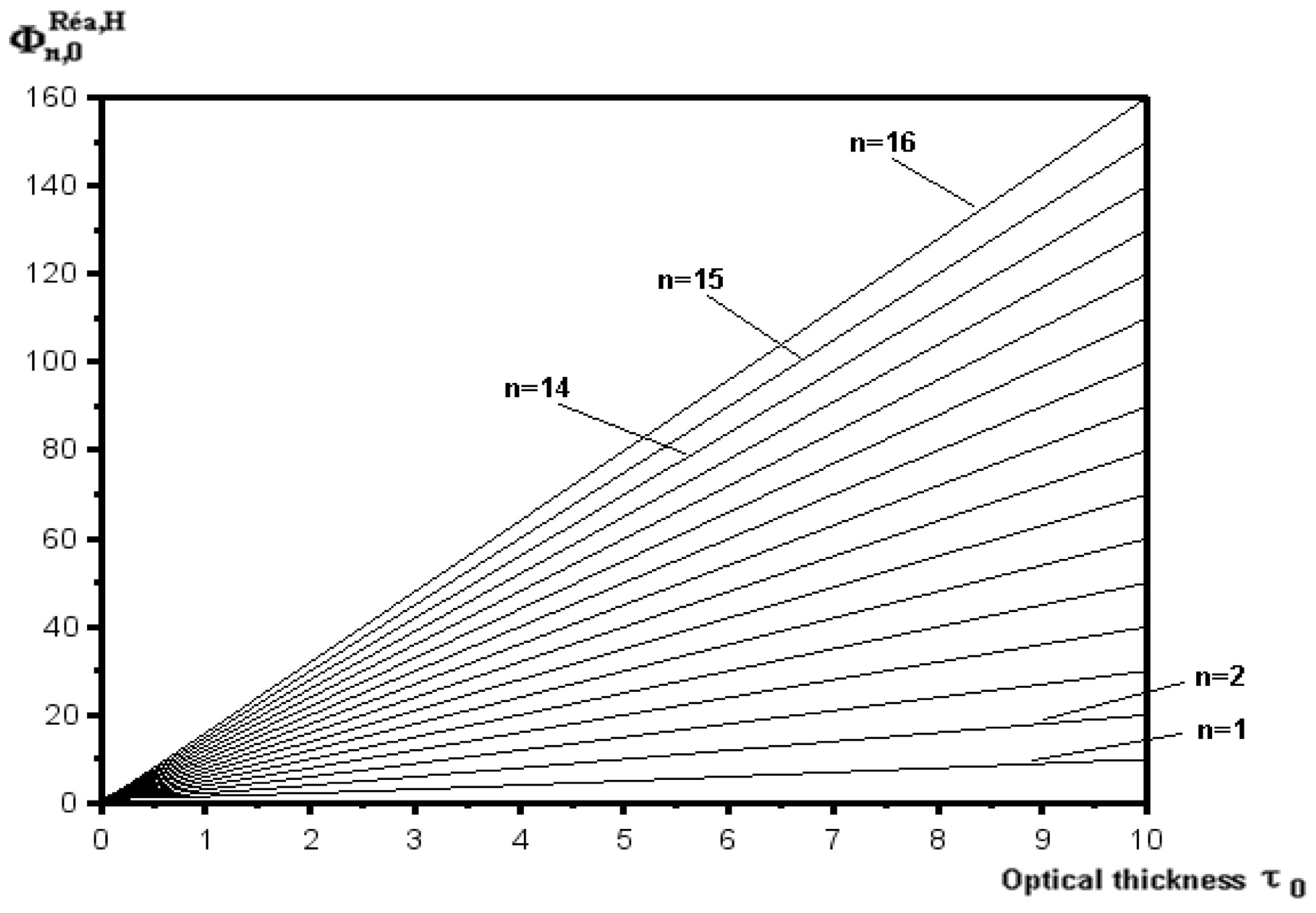
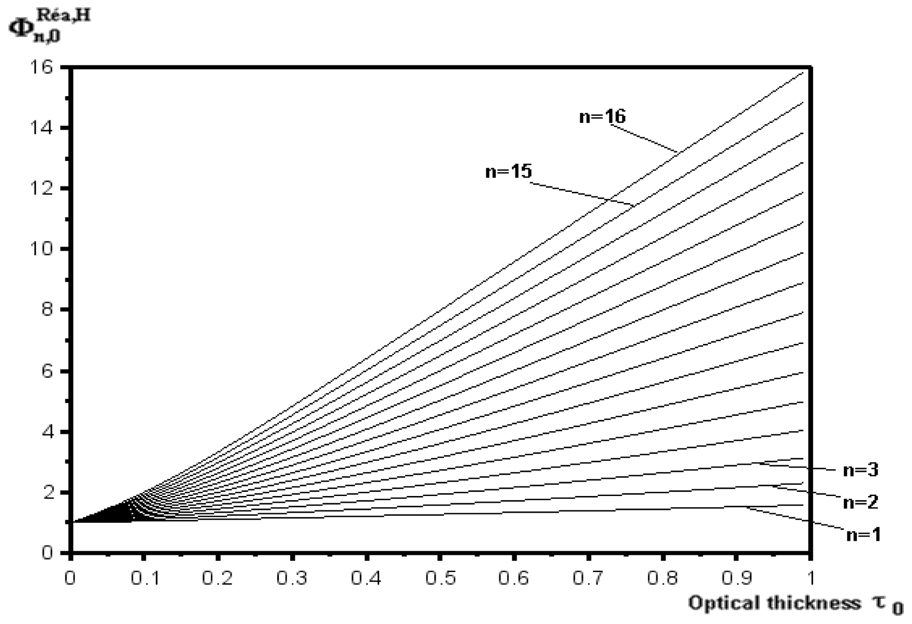
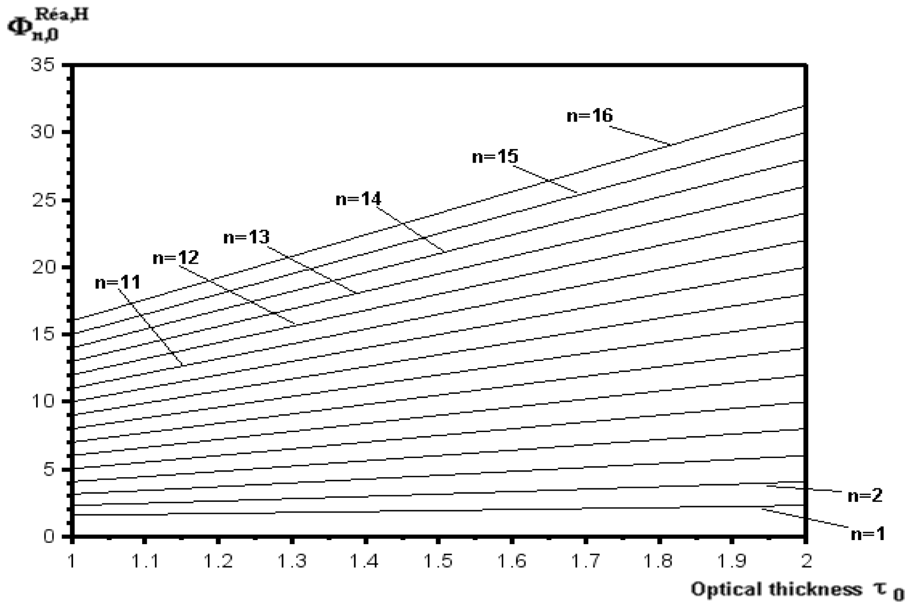
Figures 1–3 show the correction coefficient for self-absorption
 ${\it\Phi}_{n,{\it\lambda}}^{R\acute{e} a,H}$
versus optical thickness. This coefficient increases when the optical thickness increases.
Correction coefficient of self-absorption for homogeneous plasma for
 $0\leqslant {\it\tau}_{0}\leqslant 10$
.

Correction coefficient of self-absorption for homogeneous plasma for
 $0\leqslant {\it\tau}_{0}\leqslant 1$
.

Correction coefficient of self-absorption for homogeneous plasma for
 $1\leqslant {\it\tau}_{0}\leqslant 2$
.

4 Application to experimental data
4.1 Experimental details
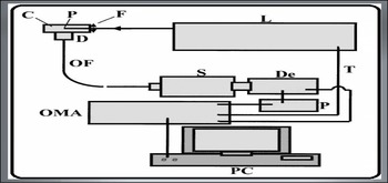
The experimental set-up is shown in figure 4. Its components are:
L: pulsed laser, F: focusing lens, C: interaction cell, T: a target when the plasma is created in the solid media, IL: optical coupler, OF: optical fibre, S: Jobin-Yvon spectrometer, D: detector, OMA2000: multichannel analyser, PC: personal computer.
The Nd : YAG laser pulse 1064 nm with an energy ranging from 10 to 115 mJ and a duration of 10 ns is focused at the centre of the cell containing water by a 50 mm focal length fused silica lens (F). The spot is approximately
 $62~{\rm\mu}\text{m}$
wide. The quartz cell, C, contains the sample and should avoid any external pollution. The light emitted by the plasma is observed at a right angle perpendicular to the path of the laser through an achromatic doublet, D, and the optical fibre, OF, to the spectrometer. The light dispersed by the spectrometer is recorded by an intensified CCD connected to a multichannel analyser.
Experimental details.

For the
 $\text{H}{\it\alpha}$
line a Jobin-Yvon spectrometer with low dispersion (240 Å mm
 $^{-1}$
) is used, while Ca narrower lines are analysed with a Chromex 500-IS (16 Å mm
 $^{-1}$
) spectrometer.
The electronic density of the plasma is determined by the Stark broadening of an emission spectral line (Ca i (422.67 nm) and the Ca ii (doublet at 393.37 and 396.85 nm)).
The LTE criterion for a stationary and homogeneous hydrogen plasma and for
 $T\approx 10\,000~\text{K}$
is:
 $N_{e}\geqslant 2.8\times 10^{17}~\text{cm}^{-3}$
(McWhirter Reference McWhirter, Huddlestone and Leonard1965). This condition is always verified in the present conditions of observation of the
 $\text{H}{\it\alpha}$
line. However, it is also necessary to check that the equilibration time for the establishment of a quasi-stationary near-LTE plasma for the hydrogen is sufficiently short compared to the
 $\text{H}{\it\alpha}$
observation time, because the laser plasmas are time dependent. It is the time needed to obtain a Boltzmann distribution for the energy over the excited states of the atoms. For the
 $\text{H}{\it\alpha}$
observation times,
 $N_{e}$
is experimentally found to be larger than
 $2.8\times 10^{17}~\text{cm}^{-3}$
and
 $T\leqslant 10\,000~\text{K}$
. The calculations (Griem Reference Griem1963) provide values smaller than 0.2 ns for the equilibration time in the present experimental conditions. Therefore, the plasma is in quasi-stationary LTE for the
 $\text{H}{\it\alpha}$
observation time.
For a Lorentzian profile, the FWHM and FWHA (full width at half-area), that represents the width at the half-area of the line, are identical. However, the maximum intensity of the line being sensitive to the dynamic effect of the ions, the determination of the electron density from the FWHA gives more accurate results. However, other authors (Parigger Reference Parigger2010) found that for measurements of
 $N_{e}$
in the order of
 $10^{17}~\text{cm}^{-3}$
and higher, the use of FWHM is preferred over the FWHA. The hydrogen
 $\text{H}{\it\alpha}$
line shape is fit well by a Lorentzian profile (Swafford & Parigger Reference Swafford and Parigger2013).
Ca and K traces are added to the pure water. This allowed us to measure the plasma diameter from the intensity variations of the Ca and K lines versus the position on the vertical axis, used to perform the Abel inversion that provides local electron density values.
A
 $x$
–
 $y$
–
 $z$
micro-positioning system allows high longitudinal (
 $z$
direction along the laser beam) and vertical (
 $y$
direction perpendicular to the laser beam) spatial resolution. Under the assumption of a cylindrical symmetry, the spectra observed versus
 $y$
are used for the numerical resolution of Abel inversion. This method allows us to obtain the local emission coefficients
 ${\it\varepsilon}^{{\it\lambda}}$
versus
 $r$
, the distance from the plasma centre.
In water the spark light intensity is much less intense than in gases (Escarguel et al. Reference Escarguel, Lesage, Ferhat and Richou2000) so it is necessary to add thousands of successive signals to significantly ameliorate the signal over the noise ratio. After each impulse, the noise is subtracted from the signal emitted. Indeed, this method gives a better result than the method based on subtracting, from 1000 spectra, 1000 figures of noise.
The Ca i (422.67 nm) and the Ca ii (doublet at 393.37 and 396.85 nm) lines are chosen to study the temperature and the electron density radial variations. However, the experimental and theoretical Ca ii doublet Stark parameters differ strongly (Konjevic & Wiese Reference Konjevic and Wiese1990), so only the electron density radial distribution normalized to the maximum density at the centre is deduced with good accuracy from this Stark broadened lines. However, in this work we took a maximum density of
 $2\times 10^{18}~\text{cm}^{-3}$
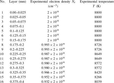
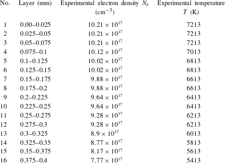
by averaging over several of values of this Stark parameters. The results of these measurements are shown in tables 1 and 2. The spectra are integrated along the line of sight for the
 $N_{e}$
and temperature measurements along the plasma. The calcium chloride salt is used to study
 $N_{e}$
temporal evolution in the longitudinal direction at different distances from the focal point towards the laser beam. The calcium chloride salt is used to study the temporal evolution of the temperature.
Experimental values of temperature
 $T$
and the experimental values of electron density
 $N_{e}$
for the
 $n$
layers. Delay from the beginning of plasma; 200 ns. Integration time; 500 ns.

Experimental values of temperature
 $T$
and the experimental values of electron density
 $N_{e}$
for the
 $n$
layers. Delay from the beginning of plasma; 355 ns. Integration time;
 $1~{\rm\mu}\text{s}$
.

Electron density radial distribution is deduced from the Stark broadened Ca ii lines. Simultaneous observation of the Ca i and Ca ii emission lines on the same spectrum provide the temperature using the Saha and Boltzmann equations (Griem Reference Griem1974; Bradt Reference Bradt2009).
The dimension of the plasma (plasma radius) so created is
 $L_{i}=0.4~\text{mm}$
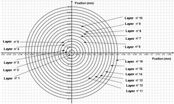
. We propose in our model to subdivide this plasma, that is considered to be cylindrically symmetric, into 16 layers of thickness of
 $L_{i}=0.025~\text{mm}$
(see figure 5).
Subdivision of the plasma section in 16 layers.

Equation (3.14) gives the correction coefficient of the self-absorption and the inhomogeneity
 ${\it\Phi}_{n,0}^{R\acute{e} a,Inh}$
at the wavelength of the line centre. For the laser-induced plasma in water studied here, this coefficient is as follows:
 $$\begin{eqnarray}\displaystyle \frac{1}{{\it\Phi}_{16,0}^{R\acute{e} a,Inh}}=\mathop{\sum }_{i=1}^{15}\left[\frac{{\it\varepsilon}_{i}^{0}}{16{\it\varepsilon}_{0}^{0}}\frac{[1-\exp (-{\it\tau}_{i}^{0})]}{{\it\tau}_{i}^{0}}\exp \left(-\mathop{\sum }_{j=i+1}^{16}{\it\tau}_{j}^{0}\right)\right]+\frac{{\it\varepsilon}_{16}^{0}}{16{\it\varepsilon}_{0}^{0}}\frac{[1-\exp (-{\it\tau}_{16}^{0})]}{{\it\tau}_{16}^{0}}.\quad & & \displaystyle\end{eqnarray}$$
For self-absorption only, the correction coefficient is:
 $$\begin{eqnarray}\displaystyle \frac{1}{{\it\Phi}_{16,0}^{R\acute{e} a}}=\frac{\displaystyle \mathop{\sum }_{i=1}^{15}\left[{\it\varepsilon}_{i}^{0}\frac{[1-\exp (-{\it\tau}_{i}^{0})]}{{\it\tau}_{i}^{0}}\exp \left(-\mathop{\sum }_{j=i+1}^{16}{\it\tau}_{j}^{0}\right)\right]+{\it\varepsilon}_{16}^{0}\frac{[1-\exp (-{\it\tau}_{16}^{0})]}{{\it\tau}_{16}^{0}}}{\displaystyle \mathop{\sum }_{i=1}^{16}{\it\varepsilon}_{i}^{0}}. & & \displaystyle\end{eqnarray}$$
For inhomogeneity only, the correction coefficient is:
 $$\begin{eqnarray}\displaystyle \frac{1}{{\it\Phi}_{16,0}^{Inh}}=\frac{\displaystyle \mathop{\sum }_{i=1}^{16}{\it\varepsilon}_{i}^{0}}{16{\it\varepsilon}_{0}^{0}}. & & \displaystyle\end{eqnarray}$$
It is easy to deduce that
 ${\it\Phi}_{16,0}^{R\acute{e} a,Inh}={\it\Phi}_{16,0}^{Inh}{\it\Phi}_{16,0}^{R\acute{e} a}$
.
 ${\it\varepsilon}_{i}^{0}$
is the emission coefficient for the
 $i$
th layer at the line centre with wavelength
 ${\it\lambda}_{0}{\it\tau}_{i}^{0}$
is the optical thickness of the
 $i$
th layer at the line centre with the wavelength
 ${\it\lambda}_{0}$
and
 ${\it\varepsilon}_{0}^{0}$
is the emission coefficient for each layer at the line centre without self-absorption. In this work we consider that
 ${\it\varepsilon}_{0}^{{\it\lambda}}={\it\varepsilon}_{1}^{{\it\lambda}}$
, because layer-1 is at the centre of the plasma, so this layer is the most emissive one.
The dominant broadening mechanism is the Stark effect, we consider that the line profile is Lorentzian. Thus from (2.5) the emission coefficient is:
 $$\begin{eqnarray}\displaystyle {\it\varepsilon}_{i}^{0}=\frac{hc}{2{\rm\pi}^{2}{\it\lambda}_{0}}AN_{Sup}^{i}L\frac{1}{{\rm\Delta}{\it\lambda}_{1/2}^{i}}. & & \displaystyle\end{eqnarray}$$
From (2.9), the optical thickness is:
 $$\begin{eqnarray}\displaystyle {\it\tau}_{i}^{0}=\frac{{\it\lambda}_{0}^{4}}{4{\rm\pi}^{2}c}N_{sup}^{i}AL\left(\exp \left(\frac{E_{sup}-E_{inf}}{kT_{i}}\right)-1\right)\frac{1}{{\rm\Delta}{\it\lambda}_{1/2}^{i}}. & & \displaystyle\end{eqnarray}$$
 $k$
is Boltzmann’s constant
 $(\text{eV}~\text{K}^{-1})$
,
 $h$
is Planck’s constant
 $(\text{J}~\text{s})$
,
 $L$
is the plasma length (m),
 $A$
is the Einstein coefficient for spontaneous emission
 $(\text{s}^{-1}),{\rm\Delta}{\it\lambda}_{1/2}^{i}$
is the full width at FWHM (m),
 ${\it\lambda}_{0}$
is the wavelength (m),
 $E_{sup}$
is the energy upper level
 $(\text{eV}),E_{inf}$
is the energy lower level
 $(\text{eV}),T_{i}$
is the temperature in the
 $i$
th layer and
 $c$
is the light celerity
 $(\text{m}~\text{s}^{-1})$
.
Posing
 $\text{cte}={\it\lambda}_{0}^{4}/(4{\rm\pi}^{2}c)AL$
, so:
 $$\begin{eqnarray}\displaystyle \frac{1}{{\it\Phi}_{16,0}^{R\acute{e} a,Inh}} & = & \displaystyle \frac{1}{16}\mathop{\sum }_{i=1}^{15}\left[\frac{{\rm\Delta}{\it\lambda}_{1/2}^{0}}{N_{sup}^{0}}\frac{\left[1-\exp \left(-\text{cte}\left(\exp \left(\displaystyle \frac{E_{sup}-E_{inf}}{kT_{i}}\right)-1\right)\displaystyle \frac{N_{sup}^{i}}{{\rm\Delta}{\it\lambda}_{1/2}^{i}}\right)\right]}{\text{cte}\left(\exp \left(\displaystyle \frac{E_{sup}-E_{inf}}{kT_{i}}\right)-1\right)}\right.\nonumber\\ \displaystyle & & \displaystyle \times \,\left.\exp \left(-\text{cte}\mathop{\sum }_{j=i+1}^{16}\left(\exp \left(\frac{E_{sup}-E_{inf}}{kT_{j}}\right)-1\right)\frac{N_{sup}^{j}}{{\rm\Delta}{\it\lambda}_{1/2}^{j}}\right)\vphantom{\frac{{\rm\Delta}{\it\lambda}_{1/2}^{0}}{N_{sup}^{0}}\frac{\left[1-\exp \left(-\text{cte}\left(\exp \left(\displaystyle \frac{E_{sup}-E_{inf}}{kT_{i}}\right)-1\right)\displaystyle \frac{N_{sup}^{i}}{{\rm\Delta}{\it\lambda}_{1/2}^{i}}\right)\right]}{\text{cte}\left(\exp \left(\displaystyle \frac{E_{sup}-E_{inf}}{kT_{i}}\right)-1\right)}}\right]\nonumber\\ \displaystyle & & \displaystyle +\,\frac{1}{16}\frac{{\rm\Delta}{\it\lambda}_{1/2}^{0}}{N_{sup}^{0}}\frac{\left[1-\exp \left(-\text{cte}\left(\exp \left(\displaystyle \frac{E_{sup}-E_{inf}}{kT_{16}}\right)-1\right)\displaystyle \frac{N_{sup}^{16}}{{\rm\Delta}{\it\lambda}_{1/2}^{16}}\right)\right]}{\text{cte}\left(\exp \left(\displaystyle \frac{E_{sup}-E_{inf}}{kT_{16}}\right)-1\right)}.\end{eqnarray}$$
From Boltzmann’s equation, we can express the upper-level density as follow:
 $$\begin{eqnarray}\displaystyle N_{sup}^{i}=\frac{g_{sup}}{Q_{z}^{i}}N_{z}^{i}\exp \left(-\frac{E_{sup}}{kT_{i}}\right). & & \displaystyle\end{eqnarray}$$
 $Q_{z}^{i}$
is the partition function of
 $z$
-state in the
 $i$
th layer,
 $N_{z}^{i}$
is the particle density in the
 $z$
-state ionization in the
 $i$
th layer
 $(\text{m}^{-3})$
and
 $g_{sup}$
is the statistical weight of the upper level.
 $$\begin{eqnarray}\displaystyle & & \displaystyle \frac{1}{{\it\Phi}_{16,0}^{R\acute{e} a,Inh}}=\frac{1}{16}\mathop{\sum }_{i=1}^{15}\left[\frac{{\rm\Delta}{\it\lambda}_{1/2}^{0}}{{g_{sup}N}_{sup}^{0}}\frac{Q_{z}^{0}}{N_{z}^{0}\exp \left(-\displaystyle \frac{E_{sup}}{kT_{0}}\right)}\right.\nonumber\\ \displaystyle & & \displaystyle \quad \times \,\frac{\left[1-\exp \left(-\text{cte}\left(\exp \left(\displaystyle \frac{E_{sup}-E_{inf}}{kT_{i}}\right)-1\right)\displaystyle \frac{g_{sup}N_{z}^{i}\exp \left(-\displaystyle \frac{E_{sup}}{kT_{i}}\right)}{Q_{z}^{i}{\rm\Delta}{\it\lambda}_{1/2}^{i}}\right)\right]}{\text{cte}\left(\exp \left(\displaystyle \frac{E_{sup}-E_{inf}}{kT_{i}}\right)-1\right)}\nonumber\\ \displaystyle & & \displaystyle \quad \times \,\left.\exp \left(-\text{cte}\mathop{\sum }_{j=i+1}^{16}\left(\exp \left(\frac{E_{sup}-E_{inf}}{kT_{j}}\right)-1\right)\frac{g_{sup}N_{z}^{j}\exp \left(-\displaystyle \frac{E_{sup}}{kT_{j}}\right)}{Q_{z}^{j}{\rm\Delta}{\it\lambda}_{1/2}^{j}}\right)\right]\nonumber\\ \displaystyle & & \displaystyle \quad +\,\frac{1}{16}\frac{{\rm\Delta}{\it\lambda}_{1/2}^{0}}{{g_{sup}N}_{sup}^{0}}\frac{Q_{z}^{0}}{N_{z}^{0}\exp \left(-\displaystyle \frac{E_{sup}}{kT_{0}}\right)}\nonumber\\ \displaystyle & & \displaystyle \quad \times \,\frac{\left[1-\exp \left(-\text{cte}\left(\exp \left(\displaystyle \frac{E_{sup}-E_{inf}}{kT_{16}}\right)-1\right)\displaystyle \frac{g_{sup}N_{z}^{16}\exp \left(-\displaystyle \frac{E_{sup}}{kT_{16}}\right)}{Q_{z}^{16}{\rm\Delta}{\it\lambda}_{1/2}^{16}}\right)\right]}{\text{cte}\left(\exp \left(\displaystyle \frac{E_{sup}-E_{inf}}{kT_{16}}\right)-1\right)}.\qquad\end{eqnarray}$$
4.2 Application to the
$\text{H}{\it\alpha}$
hydrogen line emitted by underwater laser plasma

 $\text{H}{\it\alpha}$
is a hydrogen emission line in the visible spectrum at 656 279 nm in air. It corresponds to the transition between the energy levels with principal quantum numbers
 $n=3$
and
 $n=2$
. This is the first line of the Balmer series. The study of the line broadening of
 $\text{H}{\it\alpha}$
line was performed in detail by Griem (Reference Griem1997) and more recently by Parigger et al. (Reference Parigger, Surmick, Gautam and El Sherbini2015).
The
 $\text{H}{\it\alpha}$
parameters are (NIST National Institute of Standards and Technology 1901):
 $g_{sup}=5$
 $E_{sup}=12.087506~\text{eV}$
 $E_{inf}=10.1988052~\text{eV}$
 $E_{z}=13.598434005136~\text{eV}$
 ${\it\lambda}_{0}=656.279\times 10^{-9}~\text{m}$
 $Q_{z+1}=1$
 $A_{21}=5.3877\times 10^{7}~\text{s}^{-1}$
 $$\begin{eqnarray}\displaystyle & & \displaystyle \hspace{-18.0pt}\frac{1}{{\it\Phi}_{16,0}^{R\acute{e} a,Inh}}=\frac{1}{16}\mathop{\sum }_{i=1}^{15}\left[\frac{{\rm\Delta}{\it\lambda}_{1/2}^{0}}{5N_{sup}^{0}}\frac{Q_{z}^{0}}{N_{z}^{0}\exp \left(-\displaystyle \frac{140\,269.695}{T_{0}}\right)}\right.\nonumber\\ \displaystyle & & \displaystyle \quad \times \,\frac{\left[1-\exp \left(-\text{cte}\left(\exp \left(\displaystyle \frac{21\,917.4647}{T_{I}}\right)-1\right)\displaystyle \frac{5N_{z}^{i}\exp \left(-\displaystyle \frac{140\,269.695}{T_{i}}\right)}{Q_{z}^{i}{\rm\Delta}{\it\lambda}_{1/2}^{i}}\right)\right]}{\text{cte}2\left(\exp \left(\displaystyle \frac{21\,917.4647}{T_{i}}\right)-1\right)}\nonumber\\ \displaystyle & & \displaystyle \quad \times \,\left.\exp \left(\vphantom{\frac{5N_{z}^{j}\exp \left(-\displaystyle \frac{140269.695}{T_{J}}\right)}{Q_{z}^{j}{\rm\Delta}{\it\lambda}_{1/2}^{j}}}-\text{cte}\mathop{\sum }_{j=i+1}^{16}\left(\exp \left(\frac{21\,917.4647}{T_{J}}\right)-1\right)\frac{5N_{z}^{j}\exp \left(-\displaystyle \frac{140\,269.695}{T_{J}}\right)}{Q_{z}^{j}{\rm\Delta}{\it\lambda}_{1/2}^{j}}\right)\right]\nonumber\\ \displaystyle & & \displaystyle \quad \times \,\frac{Q_{z}^{0}}{N_{z}^{0}\exp \left(-\displaystyle \frac{140\,269.695}{T_{0}}\right)}\nonumber\\ \displaystyle & & \displaystyle \quad \times \,\frac{\left[1-\exp \left(-\text{cte}\left(\exp \left(\displaystyle \frac{21\,917.4647}{T_{16}}\right)-1\right)\displaystyle \frac{5N_{z}^{16}\exp \left(-\displaystyle \frac{140\,269.695}{T_{16}}\right)}{Q_{z}^{16}{\rm\Delta}{\it\lambda}_{1/2}^{16}}\right)\right]}{\text{cte}\left(\exp \left(\displaystyle \frac{21\,917.4647}{T_{16}}\right)-1\right)}.\nonumber\\ \displaystyle & & \displaystyle\end{eqnarray}$$
Approximated by a Lorentz profile, the Stark broadening of the lines of the hydrogenoid particles is given by the following formula (Gigosos, Gonzalez & Cardenoso Reference Gigosos, Gonzalez and Cardenoso2003):
 $$\begin{eqnarray}\displaystyle {\rm\Delta}{\it\lambda}_{1/2}^{Stark}=2\times 10^{-9}\times 0.549\left(\frac{N_{e}}{10^{23}}\right)^{0.67965} & & \displaystyle\end{eqnarray}$$
 $N_{e}$
is the electron density
 $(\text{m}^{-3})$
.
For
 $L=0.4\times 10^{-3}~(\text{m})$
we are
 $\text{cte}={\it\lambda}_{0}^{4}/(4{\rm\pi}^{2}c)AL=3.377824\times 10^{-31}\;(\text{m}^{4})$
.
For the water, the molecule mass is
 $3\times 10^{-26}~\text{kg}$
and the water density is
 $1000~\text{kg}~\text{m}^{-3}$
. Thus, it is very easy to deduce that the neutral hydrogen density is:
 $N_{z}+N_{z+1}=N_{H}=(2/3)\times 10^{29}~\text{m}^{-3}$
.
 $N_{z}$
is the density of neutral hydrogen
 $(\text{m}^{-3})$
and
 $N_{z+1}$
is the density of singly ionized hydrogen
 $(\text{m}^{-3})$
.
From Saha’s equation:
 $$\begin{eqnarray}\displaystyle N_{z+1}=N_{z}\frac{1}{N_{e}}\frac{Q_{z+1}Q_{e}}{Q_{z}}\left(\frac{2{\rm\pi}m_{e}KT}{h^{2}}\right)^{3/2}\exp \left(-\frac{E_{z}-{\rm\Delta}E_{z}}{KT}\right). & & \displaystyle\end{eqnarray}$$
 $Q_{e}=2$
is the electron partition function,
 $Q_{z}$
is the partition function of neutral hydrogen,
 $Q_{z+1}$
is the partition function of singly ionized hydrogen,
 $m_{e}$
is the electron mass (kg),
 $E_{z}$
is the ionization energy of hydrogen (eV) and
 ${\rm\Delta}E_{z}$
is the reduction of ionization energy of hydrogen (eV).
By analysing several spectra in the same experimental conditions the uncertainties are estimated. Thus, a value of 15 % is found for the electron density and a value of 15 % is also found for the temperature. The uncertainties over the measured FWHM of the
 $\text{H}{\it\alpha}$
line, by using the same method, are found to be 10 %.
The partition function can be defined as a normalization factor of population densities of the energy levels. According to Boltzmann’s law and taking into account the fact that
 $\sum _{n}N_{n}=N_{z}$
, the partition function is given by the sum (Griem Reference Griem1964; Lochte-Holgreven Reference Lochte-Holgreven1968):
 $$\begin{eqnarray}\displaystyle Q_{z}=\mathop{\sum }_{n}g_{n}\exp \left(-\frac{E_{n}}{kT}\right). & & \displaystyle\end{eqnarray}$$
This sum must be made at all energy levels belonging to this ionization state
 $z$
. The problem is that this sum often diverges, and we cannot know the values of the energies of all levels. That is why it is often limited to a value
 $k$
of
 $n$
such that
 $E_{k}\leqslant E_{z}-{\rm\Delta}E_{z}$
. With the fact that we consider that only the energy level close to the ionization levels are disrupted.
This reduction is mainly due to the strong disturbance of the levels close to the ionization state. The value of this reduction in ionization energy is poorly predicted by theory, and its experimental determination is not easy because of its low value. Nevertheless, some theoretical formulas are provided for the calculation of this energy for the Saha equation and the calculation of partition functions. Two methods exist, the first is given by Unsold (Reference Unsold1955) the second is that described by Griem (Reference Griem1964), Ecker & Kroll (Reference Ecker and Kroll1966). These methods use different approaches to the calculation of the reduction in ionization energy. The reasoning of Unsold uses the fact that the issuer is disturbed by the ion nearest neighbour and leads to the relationship:
 $$\begin{eqnarray}\displaystyle {\rm\Delta}E_{z}=3z^{2/3}\frac{e^{2}}{r_{e}}. & & \displaystyle\end{eqnarray}$$
With:
 $$\begin{eqnarray}\displaystyle r_{e}=({\textstyle \frac{4}{3}}{\rm\pi}N_{e})^{-1/3} & & \displaystyle\end{eqnarray}$$
 $r_{e}$
is the average interelectronic distance.
Griem is based on thermodynamic arguments and gives the following formula:
 $$\begin{eqnarray}\displaystyle {\rm\Delta}E_{z}=(z+1)\frac{e^{2}}{{\it\rho}_{D}}. & & \displaystyle\end{eqnarray}$$
 ${\it\rho}_{D}$
is the Debye length, which is given by the following relationship:
 $$\begin{eqnarray}\displaystyle {\it\rho}_{D}=\frac{1}{e}\sqrt{\frac{KT}{4{\rm\pi}[N_{e}+\displaystyle \mathop{\sum }_{z}\mathop{\sum }_{i}(z+1)^{2}N_{z+1,i}]}}. & & \displaystyle\end{eqnarray}$$
 $e$
is elementary charge of the electron,
 $z$
is the number that describes the ionization state (
 $z=1$
for the neutral state,
 $z=2$
for the first ionization,
 $\ldots$
) and
 $N_{z,i}$
is the
 $i$
-particle density in the ionization
 $z$
-state.
The comparison of these two formulas shows that Unsold gives relatively larger the values than those of Griem.
For the hydrogen lines (NIST National Institute of Standards and Technology 1901):
 $Q_{z}=2$
for the study temperature.
 $Q_{z+1}=1$
.
 $E_{z}=13.5984~\text{eV}$
.
 ${\rm\Delta}E_{z}=7.7464\times 10^{-13}(N_{e})^{1/3}\;(\text{eV})$
.
Case 1: Delay from the beginning of plasma; 200 ns. Integration time; 500 ns.
Table 1 shows the experimental temperature
 $T_{i}$
and the experimental electron density
 $N_{e}^{i}$
for each layer for the following experimental conditions:
The laser pulses with energy
 $E=115~\text{mJ}$
are focused on water containing calcium chloride. The delay from the beginning of plasma is
 $t=200~\text{ns}$
. The integration time is 500 ns.
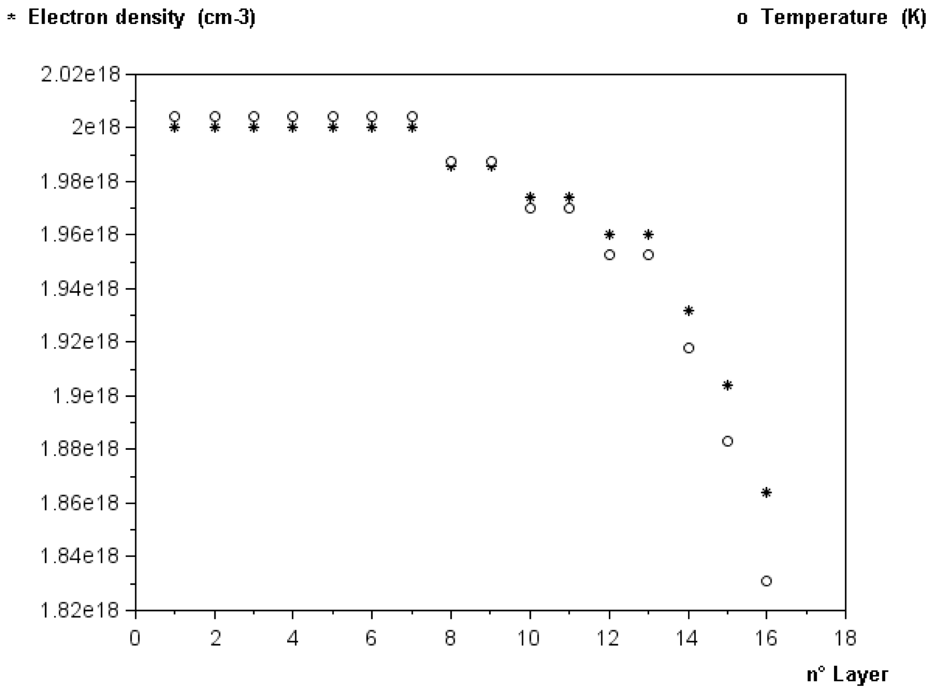
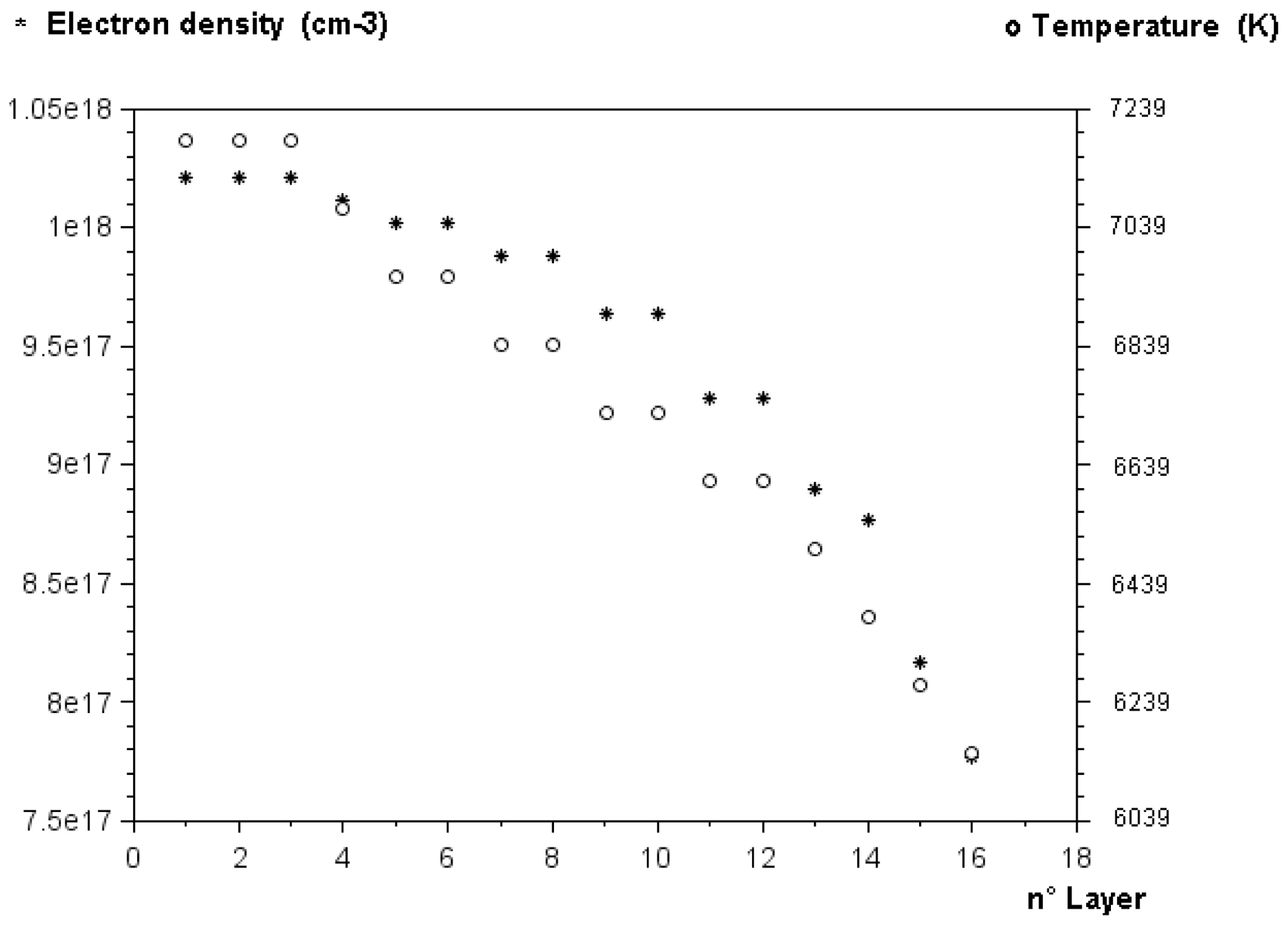
Table 1 and figure 6 show the temperature and the electron density which decrease when moving from the centre towards the plasma periphery. In fact, the centre is hotter than the periphery, producing a large electron density because of the large ionization.
Experimental values of temperature (○) and experimental values of electron density (*) in water laser plasma versus position in plasma media. Delay from the beginning of plasma; 200 ns. Integration time; 500 ns.

By utilization of (4.5), (4.2) and (4.3), the values obtained for the correction coefficients of self-absorption and inhomogeneity
 ${\it\Phi}_{16,0}^{R\acute{e} a,Inh}$
, that of self-absorption
 ${\it\Phi}_{16,0}^{R\acute{e} a}$
and that of inhomogeneity
 ${\it\Phi}_{16,0}^{Inh}$
are given in the figure 2.
These coefficients allow us to correct the line intensity of the self-absorption and inhomogeneity, the self-absorption alone or the inhomogeneity alone. The small obtained value for
 ${\it\Phi}_{16,0}^{Inh}$
indicates a relatively good plasma homogeneity. The large value of
 ${\it\Phi}_{16,0}^{R\acute{e} a}$
indicates a self-absorption effect which is not negligible. This result is very consistent with the results of (Escarguel et al.
Reference Escarguel, Lesage, Ferhat and Richou2000), for the same plasma conditions, who estimated a good spatial uniformity of the plasma.
We note that the temperature and the electron density decrease when moving from the plasma centre towards its periphery, which is logical because the centre is hotter than the periphery.
Case 2: Delay from the beginning of plasma; 355 ns. Integration time;
 $1~{\rm\mu}\text{s}$
.
Table 2 shows the temperature
 $T_{i}$
and the electron density
 $N_{e}^{i}$
for each layer, for the following experimental conditions:
The laser pulses with energy
 $E=115~\text{mJ}$
are focused in water containing calcium chloride. The delay from the beginning of plasma is
 $t=355~\text{ns}$
. The integration time is
 $1~{\rm\mu}\text{s}$
.
Table 2 and figure 7 show that the temperature and the electron density decrease when moving from the centre towards the plasma periphery. This is logical since the periphery is colder than the centre, causing a larger ionization in the centre.
Experimental values of the temperature
 $T$
and the experimental values of the electron density
 $N_{e}$
depending upon of the position of the
 $n$
layers. Delay from the beginning of plasma; 355 ns. Integration time;
 $1~{\rm\mu}\text{s}$
.

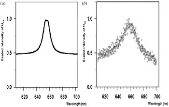
Experimental and theoretical hydrogen balmer-alpha line: (a) theoretical line (present work). (b) Experimental line (Parigger Reference Parigger2010).

The relatively low densities are due to the integration time. During the
 $1~{\rm\mu}\text{s}$
integration time, the electron density and temperature can vary significantly, but the indicated results portray average values within the temporal window.
5 Results and discussion
Figure 8 gives the
 $\text{H}{\it\alpha}$
(hydrogen balmer-alpha) line: (1) theoretical line calculated with the experimental values of electron density and temperature (present work
 $N_{e}\approx 8,5\times 10^{17}\;\text{cm}^{-3}$
). (2) Experimental line (Parigger & Oks Reference Parigger and Oks2010) (
 $N_{e}\approx 85\times 10^{17}\;\text{cm}^{-3}$
). The conditions of these two works are similar, but one experiment is in water , the other experiment is in gaseous hydrogen. However, when averaging the reported results for hydrogen gas to correspond to the gate widths considered in this work, the indicated electron density values agree. By comparison of these lines we can see (figure 8) that the two line profiles are very similar and we can deduce that the application of our method yields excellent agreement with the experimental data. For continuous radiation, we considered it a contribution that is almost half of the intensity of the
 $\text{H}{\it\alpha}$
line (which is similar to the data of Parigger & Oks (Reference Parigger and Oks2010)). The asymmetries of H-line profiles observed in some experimental spectra (figure 8
b) results mainly from inhomogeneities of ionic field and, to a lesser extent, from the static quadratic Stark effect.
By utilizing (4.5), (4.2) and (4.3), the values obtained for the correction coefficients of the self-absorption and inhomogeneity
 ${\it\Phi}_{16,0}^{R\acute{e} a,Inh}$
, that of self-absorption
 ${\it\Phi}_{16,0}^{R\acute{e} a}$
and that of inhomogeneity
 ${\it\Phi}_{16,0}^{Inh}$
are given in figure 2.
The obtained value of
 ${\it\Phi}_{16,0}^{Inh}$
indicates an inhomogeneous plasma. The value of
 ${\it\Phi}_{16,0}^{R\acute{e} a}$
indicates, a self-absorption effect which is low. These coefficients allow correcting of the line intensity of the self-absorption and inhomogeneity, the self-absorption alone or the inhomogeneity alone.
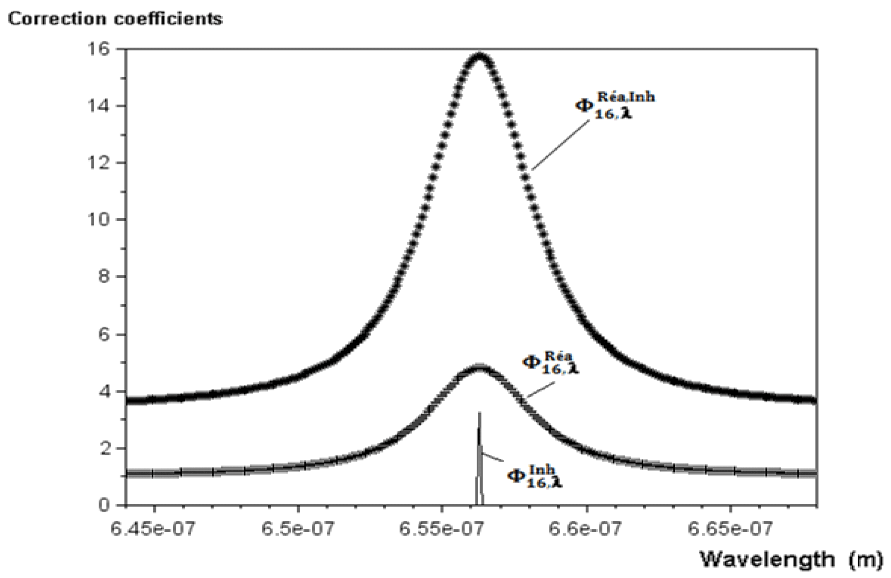
Correction coefficients of the self-absorption and inhomogeneity
 ${\it\Phi}_{16,{\it\lambda}}^{R\acute{e} a,Inh}$
, the self-absorption
 ${\it\Phi}_{16,{\it\lambda}}^{R\acute{e} a}$
and the inhomogeneity
 ${\it\Phi}_{16,{\it\lambda}}^{Inh}$
. Delay from the beginning of plasma; 355 ns. Integration time;
 $1~{\rm\mu}\text{s}$
.

Figure 9 gives the correction coefficient of self-absorption and inhomogeneity
 ${\it\Phi}_{n,{\it\lambda}}^{R\acute{e} a,Inh}$
, that of self-absorption
 ${\it\Phi}_{16,{\it\lambda}}^{R\acute{e} a}$
and that of inhomogeneity
 ${\it\Phi}_{16,{\it\lambda}}^{Inh}$
that are defined by:
 $$\begin{eqnarray}\displaystyle & \displaystyle \frac{1}{{\it\Phi}_{16,{\it\lambda}}^{R\acute{e} a,Inh}}=\mathop{\sum }_{i=1}^{15}\left[\frac{{\it\varepsilon}_{i}^{{\it\lambda}}}{16{\it\varepsilon}_{0}^{{\it\lambda}}}\frac{[1-\exp (-{\it\tau}_{i}^{{\it\lambda}})]}{{\it\tau}_{i}^{{\it\lambda}}}\exp \left(-\mathop{\sum }_{j=i+1}^{16}{\it\tau}_{j}^{{\it\lambda}}\right)\right]+\frac{{\it\varepsilon}_{16}^{{\it\lambda}}}{16{\it\varepsilon}_{0}^{{\it\lambda}}}\frac{[1-\exp (-{\it\tau}_{16}^{{\it\lambda}})]}{{\it\tau}_{16}^{{\it\lambda}}}\qquad & \displaystyle\end{eqnarray}$$
 $$\begin{eqnarray}\displaystyle & \displaystyle \frac{1}{{\it\Phi}_{16,{\it\lambda}}^{R\acute{e} a}}=\frac{\displaystyle \mathop{\sum }_{i=1}^{15}\left[{\it\varepsilon}_{i}^{{\it\lambda}}\frac{[1-\exp (-{\it\tau}_{i}^{{\it\lambda}})]}{{\it\tau}_{i}^{0}}\exp \left(-\mathop{\sum }_{j=i+1}^{16}{\it\tau}_{j}^{{\it\lambda}}\right)\right]+\frac{{\it\varepsilon}_{16}^{{\it\lambda}}}{16{\it\varepsilon}_{0}^{{\it\lambda}}}\frac{[1-\exp (-{\it\tau}_{16}^{{\it\lambda}})]}{{\it\tau}_{16}^{{\it\lambda}}}}{\displaystyle \mathop{\sum }_{i=1}^{16}{\it\varepsilon}_{i}^{{\it\lambda}}} & \displaystyle\end{eqnarray}$$
 $$\begin{eqnarray}\displaystyle & \displaystyle \frac{1}{{\it\Phi}_{16,{\it\lambda}}^{Inh}}=\frac{\displaystyle \mathop{\sum }_{i=1}^{16}{\it\varepsilon}_{i}^{{\it\lambda}}}{16{\it\varepsilon}_{0}^{{\it\lambda}}}. & \displaystyle\end{eqnarray}$$
 ${\it\varepsilon}_{i}^{{\it\lambda}}$
is the emission coefficient for the
 $i$
th layer at wavelength
 ${\it\lambda},{\it\varepsilon}_{i}^{0}$
is the emission coefficient for the
 $i$
th layer at the line centre (with a wavelength
 ${\it\lambda}_{0}$
),
 ${\it\tau}_{i}^{{\it\lambda}}$
is the optical thickness of the
 $i$
th layer at wavelength
 ${\it\lambda}$
,
 ${\it\tau}_{i}^{0}$
is the optical thickness for the
 $i$
th layer at the line centre and
 ${\it\varepsilon}_{0}^{{\it\lambda}}$
is the emission coefficient for each layer at the wavelength
 ${\it\lambda}$
without self-absorption.
The results obtained with our modelling show that inhomogeneity of layers alters only the centre of the line (as can be inferred from the shape of the coefficient of figure 9). This proves that plasma inhomogeneity is one of the causes of the inversion of spectral lines, where a hollow is observed at the centre of these lines (Amamou et al. Reference Amamou, Bois, Ferhat, Redon, Rossetto and Ripert2003; Chae Reference Chae2014). The self-absorption alters both the centre of the line and its wings.
Our model however has limitations related especially to the fact that such a plasma model with symmetrical layers with identical thickness does not represent physical reality perfectly. But it is a very interesting model for plasmas which do not exhibit strong inhomogeneities; as is the case with thermal plasmas.
6 Conclusion
Self-absorption and inhomogeneity are being widely neglected or/and their importance overlooked for plasma diagnostics. In this work, we have considered a particular spatial distribution of our plasma. In fact, we considered that our plasma is formed of
 $n$
layers, each layer is considered homogeneous and at local thermodynamic equilibrium . We thus obtained, for the first time, formulas for the correction coefficients for self-absorption and inhomogeneity, for self-absorption alone and for inhomogeneity alone. These formulas are applied to the
 $\text{H}{\it\alpha}$
hydrogen emission line, obtained from experimental spectral lines of emission of a single laser breakdown in an underwater medium. Our modelling shows that the spatial inhomogeneity alters more and principally the centre part of line, however self-absorption alters also the line wings. This modelling highlights also the fact that, due to these phenomena, the line width changes from one layer to another.
Acknowledgements
The authors would like to thank A. Lesage of GEPI ‘Observatoire de Paris’ for very interesting discussions and very valuable advice.